


Abstract
Early detection of thermal runaway in electric vehicle batteries remains challenging, and warning lead times during real-world operation are often limited. This paper proposes a hierarchical thermal runaway warning method based on an improved SegRNN model. A cross-variable self-attention module and a one-dimensional convolutional channel fusion layer are integrated into the SegRNN encoder to improve voltage prediction accuracy. One year of operational data from 23 electric vehicles of the same model, including 17 normal vehicles and 6 vehicles with confirmed thermal runaway events, is used for validation. Pearson correlation analysis is applied to select five input variables for charging and discharging conditions separately. A three-level warning strategy is developed based on voltage prediction residuals, with thresholds of 0.05, 0.12, and 0.24 V. On the test set, the proposed model achieves MAE and RMSE values of 0.48624 × 10⁻³ and 0.64961 × 10⁻³ during charging, and 3.76869 × 10⁻³ and 8.2487 × 10⁻³ during discharging, respectively. Retrospective validation on the six thermal runaway vehicles shows average warning lead times of 87.3 days for Level 1 and 2.3 days for Level 3. These results demonstrate the potential of the proposed method for early thermal runaway risk identification under real-world operating conditions.
1. Introduction
Driven by both environmental goals and the transformation of the energy structure, the new energy vehicle (NEV) industry has entered a stage of large-scale popularization [1]. As the core component providing energy supply for NEVs, the quality of the full-lifecycle battery management system (BMS) is directly related to the reliability and safety of NEVs. At present, automotive power batteries still face several challenges that need to be addressed, such as battery aging assessment [2], thermal management [3], and battery safety assurance. In addition to the battery cell itself, electric transportation is increasingly supported by more than one energy storage technology, and the resulting multi-source energy storage constraints further shape the design and operation of vehicle energy systems [4]. Among these challenges, the most critical and urgent problem is the safety problem caused by thermal runaway. The essence of thermal runaway is an irreversible thermal imbalance process, in which the internal heat generation rate exceeds the heat dissipation rate. Once triggered, it will be accompanied by a sudden temperature rise, voltage collapse, electrolyte decomposition and gas release, which may lead to combustion or explosion in severe cases [5,6]. In addition, according to multiple industry reports, thermal runaway is one of the primary causes of NEV safety accidents, and a large proportion of such accidents occur during charging or stationary stages [7]. The thermal runaway propagation process involves multi-level chain reactions from cell to module [6], with extremely severe accident consequences.
Current mainstream BMS primarily rely on fixed thresholds of parameters such as temperature and voltage to trigger alarms. However, they possess two core limitations [8]. First, the battery temperature abnormality in the early stage of thermal runaway is not obvious; relying solely on temperature thresholds makes it difficult to capture early risks in time, resulting in insufficient warning lead time and failing to reserve adequate time for intervention and disposal. Second, there is a lack of deep modeling of the temporal evolution patterns of battery states, making it difficult to distinguish between normal fluctuations and abnormal precursors, which tends to cause false alarms and missed detections [8,9]. In recent years, methods such as multi-parameter coupled warning [10], machine vision inspection [9], and acoustic-image multimodal fusion [11] have been explored for early detection of thermal runaway. However, these methods either depend on laboratory conditions or impose additional requirements on on-board sensor arrangements, making them difficult to directly transfer to large-scale real-vehicle deployment scenarios. With the deployment and application of cloud-vehicle collaborative architectures in the NEV field, the efficient collection and storage of large-scale, long-period real-vehicle operational data have become possible [12], providing a solid data foundation for data-driven early warning of thermal runaway.
Time-series prediction models are the core tools for capturing battery state evolution patterns and identifying early anomalies. To date, scholars have proposed various time-series modeling methods for power battery state prediction, including recurrent neural networks (RNNs) and their variants (LSTM, GRU), convolutional neural network-derived models (TCNs), and attention mechanism models (Transformer) [13,14]. Among them, LSTM and GRU alleviate the gradient vanishing problem of traditional RNNs through gating structures and have been widely applied in battery voltage and SOC prediction [15,16,17]; GRU also demonstrates promising estimation capability in remaining useful life prediction under electric vehicle operating conditions [16]. TCN expands the receptive field via dilated convolution, enhancing the ability to capture long-range dependencies. Transformer achieves parallel computation through the self-attention mechanism, improving training efficiency, and has been applied to battery life prediction [18]. In addition, some studies have explored strategies combining signal decomposition with deep learning, such as using CEEMDAN to decompose capacity degradation curves followed by Bi-LSTM for SOH prediction [19], and enhancing prediction stability through wavelet denoising and attention mechanisms [20], providing useful ideas for battery state estimation under complex operating conditions. Progress has also been made in SOH and remaining useful life prediction methods based on real-vehicle data, where high-accuracy state estimation can be achieved through dynamic voltage interval selection and multi-dimensional fusion models [21]. Some studies have further proposed deep learning hybrid models based on reconstructed voltage/current curves [22], model ensemble frameworks adapted to different charging voltage segments [23], and prediction methods utilizing transfer learning on real-vehicle charging data [24], enriching the application scenarios of data-driven methods in battery management. However, the above models still have shortcomings in the battery thermal runaway warning scenario: battery operational data are characterized by multi-channel coupling, strong noise interference, and non-stationary evolution. Traditional models struggle to adequately characterize the dynamic correlations among variables, leading to insufficient prediction accuracy of healthy voltage and an inability to precisely identify the subtle voltage anomalies in the early stage of thermal runaway.
The segmented recurrent neural network (SegRNN), through its segmented recurrent encoding and parallel multi-step decoding strategy, reduces the computational complexity of long-sequence modeling while mitigating the gradient propagation problem. However, its original structure adopts a channel-independent modeling approach, which cannot fully exploit the coupling information among multiple battery variables, thus limiting prediction accuracy [20,25]. Regarding pre-event thermal runaway prediction, some scholars have employed interpretable machine learning methods to predict thermal runaway severity in advance [26], as well as deep learning-based adaptive early warning for charging and discharging processes [27], verifying the feasibility of data-driven methods in thermal runaway warning. Nevertheless, substantial room for improvement remains in terms of warning lead time and graded handling strategies.
In these studies, there are three limitations. First, comparative evaluation is usually reported in the form of point prediction errors (RMSE, MAE and R2) only under a single operating condition, while charging and discharging are dominated by different excitation sources, so it is necessary to construct input variable sets for each operating condition [12,13,21]. Second, channel-independent sequence models, such as the original SegRNN, process each variable independently and do not explicitly capture inter-variable dependencies [20,25]. Third, the prediction residual is only considered as an anomaly indicator, and rarely converted into an explicit rule between the residual size and the warning level [26,27]. These three limitations define the gap to be solved in this paper: the channel-independent sequence model cannot use the coupling information between the battery channels, and the voltage residual warning has not yet been included in the hierarchical warning strategy.
To solve the above questions, this paper makes three contributions: (1) The SegRNN encoder is extended by adding a cross-variable self-attention module and a one-dimensional convolutional channel fusion layer. Both of them explicitly model the coupling relationship between the channels of the battery while retaining the original architecture of segmented cyclic coding and parallel multi-step decoding. (2) Based on the residual between the measured voltage of each cell and its predicted healthy voltage, a three-level early warning rule is defined, and the thresholds are 0.05 V, 0.12 V and 0.24 V, respectively. (3) The proposed method is verified on 23 real vehicles with more than 1 year of operation data, and 6 of them have experienced thermal runaway; the prediction accuracy is compared with seven baseline models under charging and discharging conditions, and the six thermal runaway vehicles are evaluated by back-tracking warning.
2. Methodology
High-quality data are the foundation of time-series modeling and risk warning. The research data in this paper originate from a cloud-vehicle collaborative platform. These data suffer from problems such as missing values, outliers, and unstructured fields, necessitating systematic preprocessing to construct a high-quality time-series dataset suitable for the thermal runaway warning task. Section 2.1 describes the data source, Section 2.2 describes the preprocessing process, Section 2.4, Section 2.5 and Section 2.6 describe the voltage prediction model, and Section 2.7 describes the experimental scheme. The warning rule itself is given in Section 3.
2.1. Data Source and Basic Information
The experimental data consist of continuous operational data from 23 electric passenger vehicles of the same model, covering the period from early June 2024 to the end of July 2025, with a sampling interval of 2 s. Among these vehicles, 17 are normally operating vehicles, and 6 are vehicles with thermal runaway. The data include multiple categories of fields such as vehicle operating status, key parameters of the power battery, cell voltage and temperature data, and environmental parameters. The data characteristics of long period, same vehicle model, and multiple vehicles provide sufficient data support for risk model training, threshold calibration, and cross-vehicle retrospective validation.
2.2. Data Preprocessing Procedure
For the thermal runaway warning task, data preprocessing must satisfy three fundamental requirements: time alignment, field parsability, and sample modelability. The data preprocessing is performed in Python 3.10.11. Pandas 2.3.3 and NumPy 1.26.4 are used for data processing and parsing concatenated cell voltage and temperature strings. Matplotlib 3.10.9 is used to generate diagnostic plots.
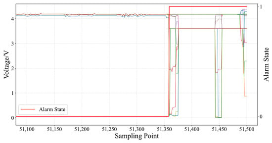
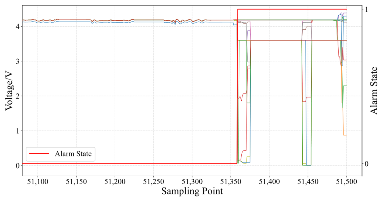
First, time alignment between alarm information and operational data is performed. Since historical operational data and alarm data are stored in separate tables on the platform side, the alarm start time and end time need to be mapped onto the operational data timeline. Then, an alarm label column is constructed to accomplish the temporal localization of risk samples, as shown in Figure 1. If a clear alarm exit time exists, samples within the alarm interval are labeled as 1 (risk samples) and the remaining samples are labeled as 0 (normal samples). If the exit time is missing, all samples from the alarm start time to the end of that data upload session are labeled as 1, so as to ensure that no risk sample is omitted.
Figure 1.
Alarm status and battery voltage after time alignment.
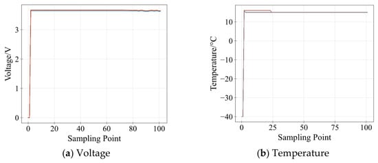
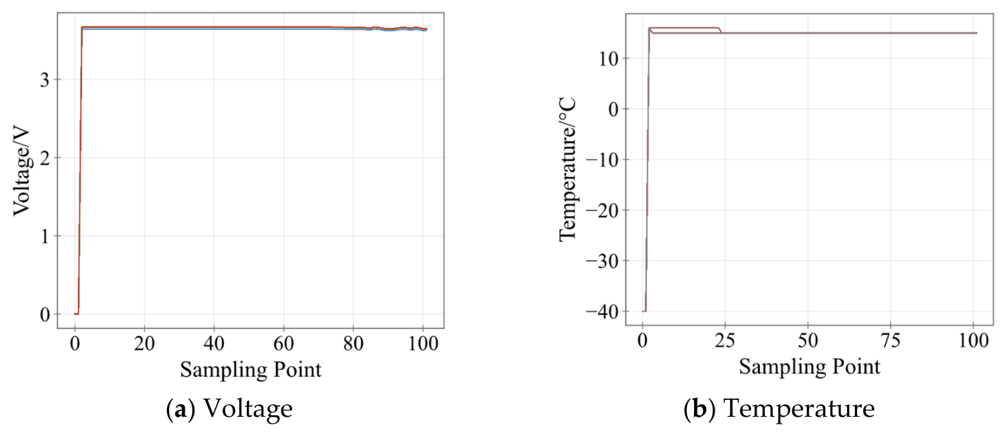
Second, abnormal data and invalid data are removed. Addressing the issues of channel default values (e.g., 0 V, −40 °C) occurring during the vehicle power-on initialization phase and missing values in key fields, such records are mostly concentrated at the beginning of a single upload cycle and do not reflect the actual battery state, as shown in Figure 2. They are directly eliminated to prevent spurious signals from being introduced into model training. Meanwhile, the cell voltage and temperature probe data stored in concatenated string format are parsed into a structured matrix and probe vectors. The extreme values together with their index fields are retained to support subsequent risk cell localization and consistency verification.
Figure 2.
The issues of channel default values (e.g., 0 V, −40 °C) occurring during the vehicle power-on initialization phase.
Finally, segment-based sample construction is performed. Since the vehicle model does not support regenerative braking, driving–charging segments are excluded due to their limited relevance to thermal runaway warning. Records corresponding to the charging completion state are also removed. Therefore, only two types of segments are retained: stationary charging and non-charging (discharge-dominant) segments. To reduce the influence of short sequences on model training, segments containing fewer than 300 records are discarded. This corresponds to approximately 10 min at a sampling interval of 2 s. After preprocessing, 1286 charging segments and 3452 discharging segments are obtained, resulting in a total of 4738 valid segments. These segments are used for subsequent time-series modeling and thermal runaway warning.
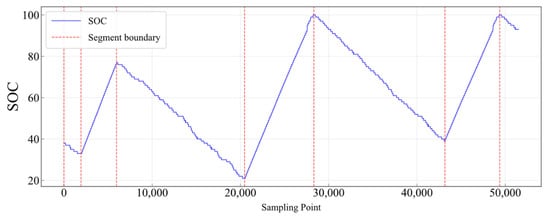
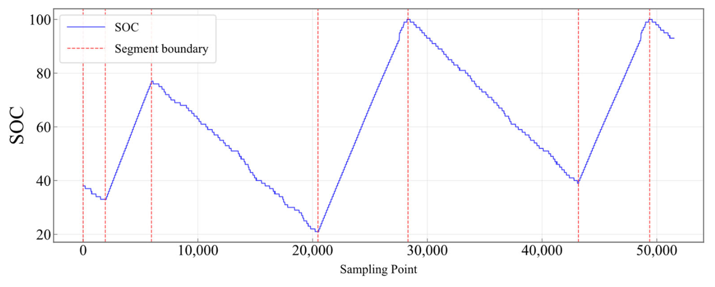
Figure 3 is a sketch of the segmentation process following data processing. It shows the state of charge (SOC) of a single vehicle in a representative period containing several normal charge and discharge cycles. The vertical dashed line marks the segmented boundary obtained through the above process. In the figure, the increase in SOC indicates the charging process, and the decrease in SOC indicates the discharging process. The figure is used to illustrate how to separate the static charging section and the non-charging (discharge-dominant) section.
Figure 3.
Segment-based sample construction process.
2.3. Feature Screening and Data Normalization
Vehicle operational data contain a large number of state variables, yet not all variables provide effective information for the temporal evolution of battery voltage. High-dimensional redundant inputs tend to introduce collinearity interference, amplify noise propagation, and weaken the generalization stability of the model. Therefore, it is necessary to select variables strongly correlated with the target voltage (median cell voltage, V_median) as model inputs through feature screening.
In this paper, the Pearson correlation coefficient is adopted to measure the linear statistical dependence between the candidate input X and the target output (V_median), whose definition is given in Equation (1).
where and are the -th sample values of the input variable and the target output, respectively; and are the mean values of the input variable and the target output; and is the number of samples. Correlation characterizes statistical dependence rather than causality between variables, but it can serve as an effective prior for eliminating information redundancy and screening candidate variables.
The energy flow, control strategies, and dominant excitation sources differ between charging and discharging conditions. During charging, the battery voltage response is mainly governed by the charging strategy, whereas during discharging, it is strongly influenced by load demand and driving behavior. Combining data from these two conditions may obscure their distinct relationships and lead to misleading correlation estimates. Therefore, Pearson correlation analysis is performed separately for charging and discharging segments, and input features are selected independently for each condition.
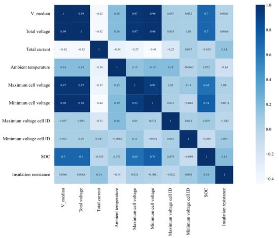
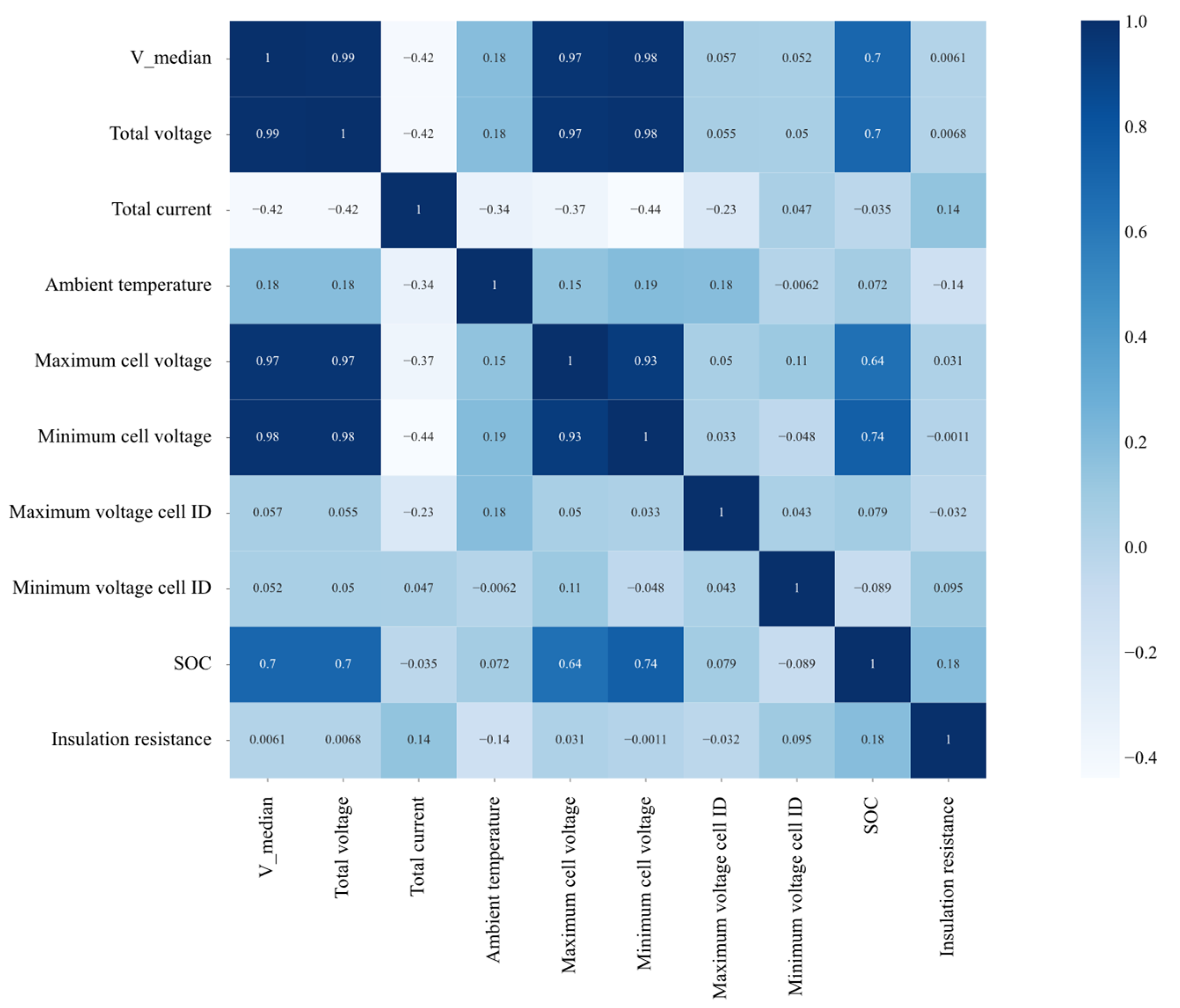
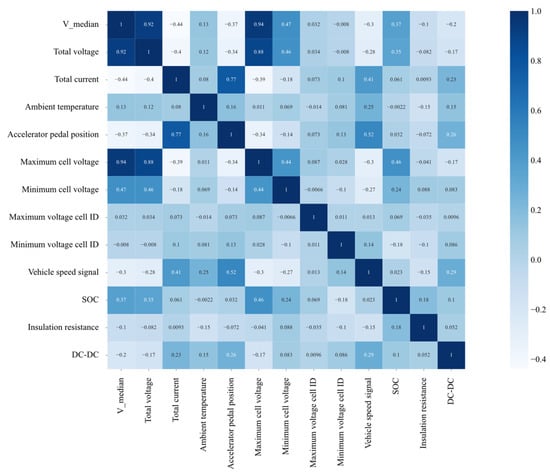
Under the charging state, the vehicle speed is constantly zero, and the vehicle state and DC-DC state remain stable, thus belonging to approximately constant variables. Since the Pearson correlation coefficient is sensitive to fluctuations, the correlation calculation for such variables lacks statistical significance and would increase redundant dimensions. Hence, they are eliminated. The correlation analysis results show that the variables highly correlated with V_median include total voltage, maximum cell voltage, minimum cell voltage, total current, and SOC, as shown in Figure 4. These variables are selected as the input features for V_median prediction under the charging condition.
Figure 4.
Pearson correlation coefficients for charging segments.
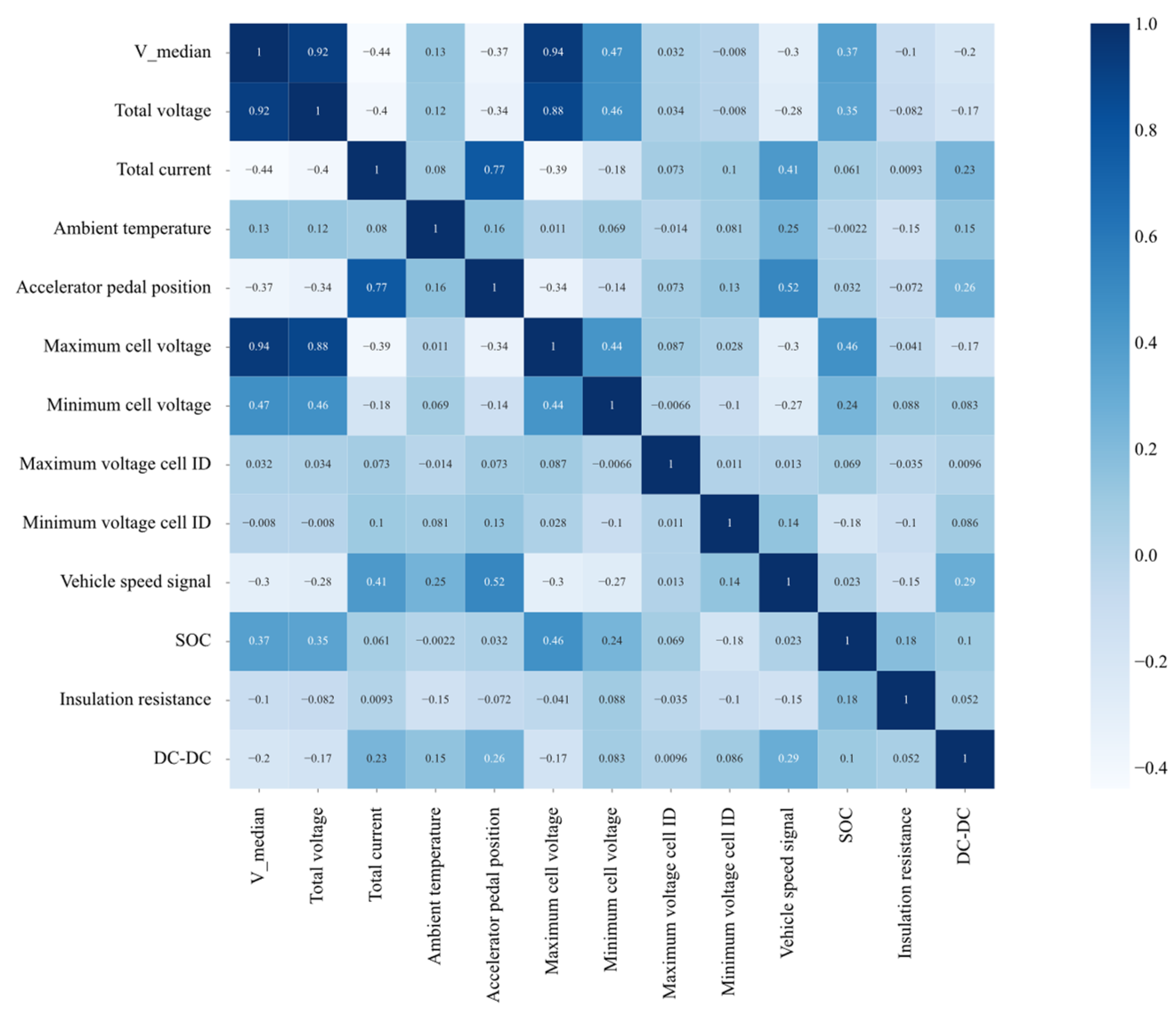
Under the discharging state, variables such as vehicle speed, pedal position, and DC-DC operating state vary with vehicle operation. These variables provide information about load variations and system operating conditions. The correlation analysis results show that the variables highly correlated with V_median include total voltage, accelerator pedal position, vehicle speed, total current, and SOC. Considering that under the discharging condition, a faulty cell may cause abnormal jumps in the maximum and minimum cell voltages, thereby introducing fault signal leakage and impairing the model’s ability to learn the healthy voltage baseline, and that extreme value features are sensitive to anomalies and prone to causing training instability, the maximum and minimum cell voltages are excluded. Consequently, total voltage, accelerator pedal position, vehicle speed, total current, and SOC are finally selected as the input features for V_median prediction under the discharging condition, as shown in Figure 5.
Figure 5.
Pearson correlation coefficients for discharging segments.
The input variables have different physical units and numerical scales, such as current in A, voltage in V, SOC in %, and vehicle speed in km/h. Directly using these variables without normalization may cause features with larger numerical values to dominate model training. This can affect training stability and reduce the contribution of features with smaller numerical scales. To eliminate scale discrepancies, min-max normalization is applied to the input sequences, mapping all variables to the [0, 1] interval, as shown in Equation (2).
where denotes the normalized data, is the original input parameter value, and and are the minimum and maximum values of that input variable, both estimated on the training set. Through normalization, each input variable is ensured to have equal weight during model training, thereby enhancing the training stability and convergence speed of the model.
These two values are calculated based only on the training data and then applied intact to the validation and test sets, so normalization is a fixed, time-invariant, variable-by-variable scaling: it does not use any information from the validation or test sets, nor any observations from the predicted time or subsequent time steps. The above Pearson-based feature screening is also only fitted on the training set.
The voltage anomalies in the early stage of thermal runaway are characterized by their concealed and precursory nature. Accurately predicting the temporal evolution patterns of healthy battery voltage is the core of identifying voltage anomalies and achieving prospective thermal runaway warning. This section first evaluates several representative time-series prediction models. Based on the characteristics of battery data, including cross-variable dependencies, noise, and non-stationarity, an improved SegRNN model is then developed for battery voltage prediction.
SegRNN employs segmented recurrent encoding and parallel multi-step decoding to reduce the number of recurrent updates in long-sequence prediction. This design shortens gradient propagation paths and improves computational efficiency compared with conventional RNN architectures. However, the original SegRNN adopts a channel-independent modeling strategy, which processes each variable separately and does not explicitly capture inter-variable dependencies. This limitation may restrict its ability to exploit complementary information from multiple battery variables and further improve voltage prediction accuracy.
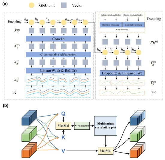
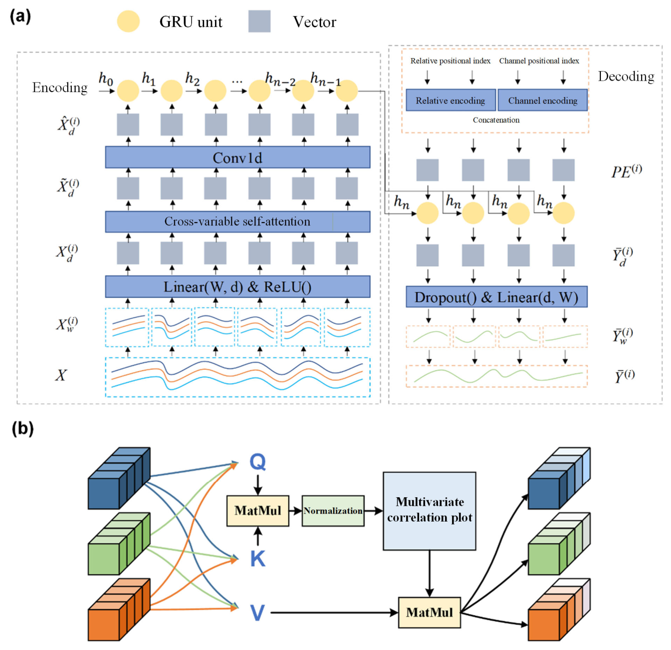
Based on the above analysis, under the premise of retaining the efficient time-series modeling framework of SegRNN, structural improvements are made to the multi-channel feature modeling approach in the encoding stage. A feature optimization module combining cross-variable self-attention and channel fusion is introduced to enhance the model’s ability to characterize the multi-variable coupling relationships of the battery. The overall architecture of the improved SegRNN model is shown in Figure 6. The following sections are expanded according to the data flow of the model: segmented projection and cross-variable self-attention (Section 2.4), channel fusion and segmented cyclic coding (Section 2.5), and parallel decoding and prediction output (Section 2.6).
Figure 6.
Architecture of the improved SegRNN. (a) Improved overall process of the model: time segmentation of multivariate input, learnable segmented projection, cross-variable self-attention, one-dimensional convolutional channel fusion, GRU-based segmented cyclic coding, and parallel multi-step decoding of the target voltage sequence. (b) Details of the cross-variable self-attention module, where the query, key, and value matrices are constructed along the variable dimension in each time segment.
2.4. Segmented Projection and Cross-Variable Self-Attention Modeling
Assume that the battery state information within a historical time window is represented as a multivariate observation sequence , where is the length of the historical sequence and denotes the variable dimension, corresponding to state parameters such as total voltage, total current, and SOC.
To reduce the computational complexity of recurrent modeling under long-sequence conditions and to enhance the model’s ability to perceive local temporal evolution patterns, the original time series is divided into consecutive segments with a fixed window length . The number of segments is . The -th temporal segment is denoted as . Through temporal segmentation, the model shifts its focus from the instantaneous changes at a single time point to characterizing the overall evolution features within a time interval, thereby suppressing the adverse effects of high-frequency noise on prediction performance to a certain extent.
For the variable sequence within each segment, a learnable linear projection mapping is introduced along the temporal dimension to transform the time series within the segment into compact feature embeddings, as shown in Equation (3).
where is a learnable weight matrix and denotes the hidden feature dimension. The projected can be regarded as each variable in the -th temporal segment corresponding to a -dimensional embedding vector, achieving dimensionality reduction and compression along the temporal dimension while enhancing the discriminability of segment-level feature representations, thereby providing a compact representation for subsequent cross-variable modeling and recurrent encoding.
For the embedding representation of the -th temporal segment, the query (), key (), and value () matrices are constructed, as shown in Equation (4), to explicitly model their mutual dependencies in the variable dimension through the cross-variable self-attention mechanism.
where , , and are the learnable weight matrices for , , and , respectively. The output of the cross-variable self-attention for the -th time segment is calculated by
where is the hidden feature dimension defined in Equation (3). The cross-variable self-attention mechanism captures the relationships among different variables within each temporal segment. It adaptively assigns attention weights to emphasize variables that are more relevant to voltage prediction. This helps reduce the influence of redundant or noisy information.
To ensure training stability and feature distribution consistency, a feature representation incorporating residual connection and layer normalization is introduced by
2.5. Channel Fusion and Segmented Recurrent Encoding
After completing the cross-variable dependency modeling, a one-dimensional convolutional feature optimization layer is introduced to perform global linear fusion and dimensionality compression on the attention-enhanced multivariate features, as shown in Equation (7). This convolution operation is equivalent to performing a learnable weighted aggregation along the variable dimension, forming a compact and robust segment-level feature representation while preserving the cross-variable interaction information, thereby reducing the computational complexity of the subsequent recurrent encoding.
The fused segment-level features are sequentially fed into a GRU unit for recurrent modeling to capture the temporal dependencies between segments. The update process of the GRU unit is shown in Equation (8). Through the coordinated operation of the update gate and reset gate, the retention and forgetting of historical information are flexibly adjusted, thereby enhancing the capability to capture long-range dependencies.
where denotes the update gate, denotes the reset gate, denotes the candidate hidden state, denotes the current hidden state, , , and are learnable weight matrices, is the sigmoid activation function, and is the hyperbolic tangent activation function. After recurrent iterations (t = 1, …, n), the final hidden state comprehensively encodes the evolution characteristics of the historical multivariate sequence over the entire time horizon.
2.6. Parallel Decoding and Prediction Output
In the decoding stage, a target voltage sequence of length needs to be predicted, which is divided into segments according to the window length . To address the issue of segment order loss caused by the elimination of recurrence during decoding, corresponding position embeddings are generated to explicitly provide segment index and channel identity information. Each position embedding is constructed by concatenating a relative positional encoding (representing the position of each predicted segment within the complete sequence) and a channel positional encoding (representing the position of the current channel within the multi-channel sequence), as shown in Figure 7, thereby alleviating the problem of insufficient cross-variable relationship characterization caused by the channel-independent strategy and enhancing the prediction accuracy of the model.
Figure 7.
The position embedding for the target sequence .
The decoding stage shares the same GRU unit with the encoding stage. The final hidden state obtained from the encoding stage is combined with the position embeddings , and they are jointly fed into the shared GRU unit in parallel. The length of each input vector is , denoted as . Since the predicted segments are independent of each other during the decoding process, this parallel decoding strategy not only achieves intra-sample parallel computation, significantly improving inference efficiency, but also structurally avoids the cumulative propagation of prediction errors along the temporal dimension.
Finally, passes through a Dropout layer, which randomly drops a certain proportion of parameters to achieve regularization and prevent model overfitting. It is then transformed into via a learnable linear prediction layer , and reshaped into as the final voltage prediction result.
2.7. Experimental Environment and Evaluation Protocol
All experiments were run in Python 3.10.11, using PyTorch 2.5.1 (CUDA 12.1, cuDNN 9.1.0), pandas 2.3.3, NumPy 1.26.4, scikit-learn 1.7.2 and Matplotlib 3.10.9. The hardware environment was an Intel Core i7-12700H CPU and an NVIDIA RTX 3060 GPU. The dataset is divided into a training set, a validation set, and a test set. A strict vehicle-level holdout is adopted. The 23 vehicles were divided into 15 training vehicles, 3 validation vehicles and 5 test vehicles. The training set contains only normal vehicles, while the validation set and test set contain all six thermal runaway vehicles and the remaining normal vehicles. No vehicle will appear in multiple subsets. The number of charging and discharging segments in each subset was 3413 (72.0%), 421 (8.9%) and 904 (19.1%), respectively. A sliding window with a length of = 24 and a step size of 1 is used in each segment. The model is trained using the Adam optimizer with a learning rate of 0.0001, a maximum of 100 training epochs, and an early stopping mechanism with a patience value of 10. The performance was reported by mean squared error (MSE), root mean square error (RMSE), mean absolute error (MAE) and coefficient of determination (R2). The closer the R2 value is to 1, the better the model fitting is, while the smaller the MSE, RMSE and MAE values are, the higher the prediction accuracy is. The key hyperparameters for improving SegRNN are listed in Table 1.
Table 1.
Key hyperparameters of the improved SegRNN used in this study.
3. Hierarchical Thermal Runaway Warning Strategy
Based on the healthy voltage prediction results obtained from the improved SegRNN model, a thermal runaway risk grading rule based on prediction residuals is constructed to achieve prospective identification and graded handling of thermal runaway risk, thereby forming a closed-loop chain of “prediction–residual calculation–risk determination–warning output”.
3.1. Voltage Anomaly Mechanism of Thermal Runaway Precursors
Thermal runaway typically occurs when the battery is in a high-energy state with limited heat dissipation. Typical triggering mechanisms include manufacturing defects in battery cells, micro-short circuits caused by localized damage, and the resulting localized Joule heat accumulation. Based on the real-vehicle after-sales data in this study, all thermal runaway events occurred after charging completion, at which point the battery was in a high-energy state with relatively high energy density and a low safety margin. If there are latent defects inside the battery (such as separator defects or localized damage caused by long-term use), a micro-short circuit inside the cell may be induced, with current concentrating through the defective area and causing localized overheating. If the heat dissipation condition is insufficient, the localized high temperature will gradually spread, promoting electrolyte decomposition and severe side reactions between the cathode and anode materials, releasing a large amount of heat, and forming a positive feedback mechanism of “local overheating–intensified side reactions–heat accumulation”, which ultimately triggers thermal runaway.
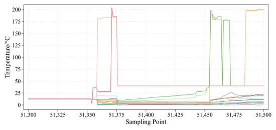
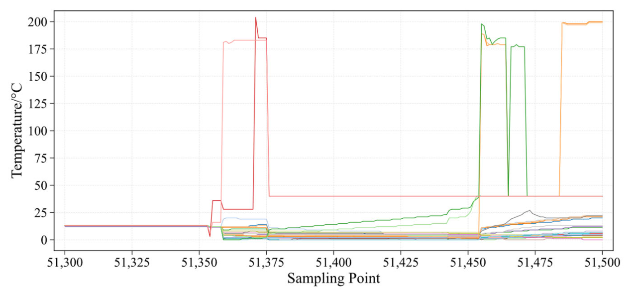
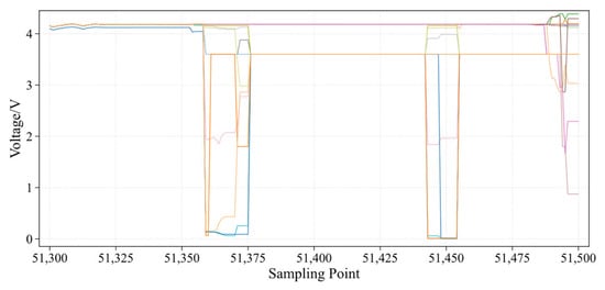
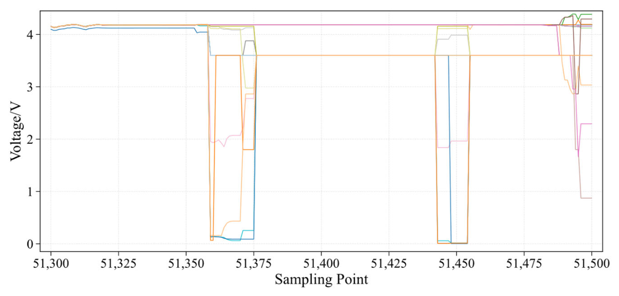
From the perspective of phenomenon identification, there is often a lack of obvious temperature abnormality in the early stage of thermal runaway, as shown in Figure 8. Real-vehicle data verification shows that before thermal runaway occurs, the temperature curves of individual cells remain relatively stable without significant differences, making it difficult to promptly identify cell anomalies based solely on temperature changes. However, from the perspective of cell voltage curves, as shown in Figure 9, while other cells are still in a normal state, the faulty cell has already shown signs of a voltage drop, which is a typical characteristic of an internal short circuit. As the voltage drop continues to develop, this cell ultimately becomes the initiation point of thermal runaway. Therefore, voltage anomaly is the most precursory characteristic in the early stage of thermal runaway and can serve as the core indicator for prospective thermal runaway warning.
Figure 8.
Temperature values at the moment of thermal runaway.
Figure 9.
Voltage values at the moment of thermal runaway.
3.2. Risk Grading Determination and Warning Rules
Based on the improved SegRNN model, the preprocessed battery multi-channel time-series data are input to obtain the predicted voltage response of healthy individual cells under the current operating condition, which serves as the voltage reference baseline. The real-time measured voltage of each cell is compared with the predicted voltage , and the prediction residual is calculated, as shown in Equation (9), to quantify the degree of abnormal deviation of each cell from the healthy state.
The regression target of the model is the median voltage V_median of the battery pack, so the model generates a predicted value at each time step. The predicted value represents the voltage that a healthy battery should perform under the current operating condition and is used as a common health voltage baseline for each cell: The baseline for any cell is the same predicted value , regardless of which cell is considered. The measured voltage V of each cell is compared with the baseline, and the residual is evaluated according to Equation (9). The unit whose residual exceeds the warning threshold is identified as the fault unit and triggers the corresponding warning level. Therefore, the cell index depends on which cell crosses the threshold and does not require a separate cell regression model.
A larger prediction residual indicates a more significant deviation of the cell voltage from the healthy state and a higher probability of fault or thermal runaway risk.
To achieve refined safety management, a three-level warning mechanism is constructed. The determination thresholds, warning information, and disposal strategies for each warning level are specified below.
Three warning levels are defined based on the prediction residuals. When 0.05 V ≤ < 0.12 V, a Level 1 (low-risk) warning is issued; the unit is marked as a suspected fault unit, and it is recommended that the owner go to the service station to check the self-discharge and contact resistance in order to identify and mitigate the risk early. The Level 2 (medium risk) warning corresponds to 0.12 V ≤ < 0.24 V, indicating that there is a significant cell anomaly consistent with the early internal short circuit. Mitigation measures related to this level, that is, limiting high-rate charge and discharge to reduce thermal stress and issuing emergency maintenance notices, are described as conceptual strategies; their effectiveness has not been verified in this study. The Level 3 (high-risk) warning corresponds to ≥ 0.24 V, and it is determined that the cell is approaching the critical state. The mandatory measures proposed for this level, that is, cutting off charging, limiting vehicle operation and activating the active cooling system, are also conceptual, and their effects cannot be quantified with existing data. These measures must be verified before they are proposed as verified control functions.
These three warning thresholds are not derived from pure statistical criteria. They are jointly determined by the vehicle manufacturer and the author according to the alarm requirements specified for the battery system, and these three residual ranges correspond to the graded alarm levels required by the specification.
This hierarchical warning strategy realizes a closed-loop chain from anomaly identification to risk disposal, capable of capturing voltage precursors before thermal runaway enters the rapid temperature rise stage, thereby reserving a sufficient time window for risk intervention.
4. Real-Vehicle Retrospective Validation and Results Analysis
4.1. Retrospective Validation on Thermal Runaway Vehicles
Based on the proposed hierarchical warning strategy, retrospective validation is conducted on the six thermal runaway vehicles, focusing on analyzing the warning lead time and the accuracy of risk cell localization. The retrospective results for some vehicles are shown in Table 2.
Table 2.
Warning lead time and warning cell ID of all thermal runaway vehicles.
In this study, the warning lead time is defined as the interval between the warning time generated by the proposed method and the actual thermal runaway alarm time recorded by the vehicle. The warning time is determined from historical operational data, while the actual alarm time is obtained from the vehicle records. Therefore, the warning lead time is evaluated retrospectively for each vehicle with confirmed thermal runaway, and each warning level is assessed separately.
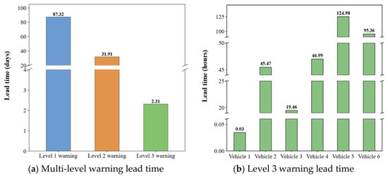
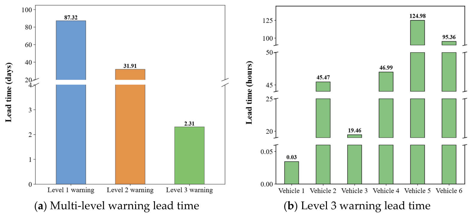
For each vehicle with confirmed thermal runaway, the warning lead time is calculated as the difference between the actual thermal runaway alarm time and the first warning time at each level. As reported in Table 2, the Level 1 warning lead times for VIN 1 to VIN 6 are 17.1, 41.9, 102.8, 117.5, 127.3, and 117.2 days, respectively. The average Level 1 warning lead time is therefore 523.8/6 = 87.3 days. Similarly, the Level 3 warning lead times are 0.0, 1.9, 0.8, 2.0, 5.2, and 4.0 days, respectively, with an average of 2.3 days. The corresponding results are presented in Figure 10. For the approximate time indicated as “Afternoon” in the table, 12:00 is used as the reference time. Shifting this time by several hours would have a negligible effect on the calculated warning lead time.
Figure 10.
Retrospective warning results of thermal runaway vehicles.
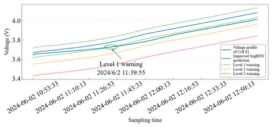
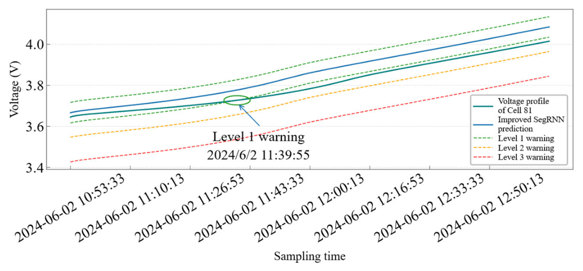
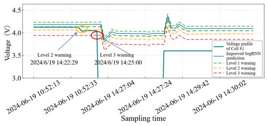
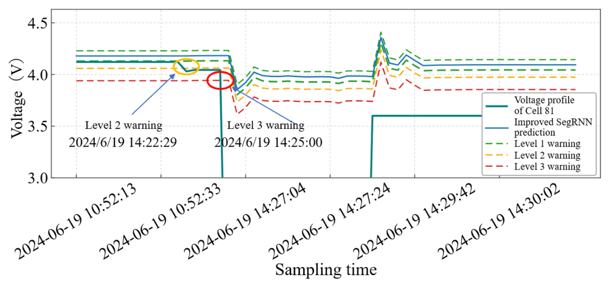
Taking the thermal runaway vehicle with VIN 1 as an example, as shown in Figure 11, the system captured the abnormal signal of Cell 81 at 11:39:55 on 2 June 2024, and issued a Level 1 warning. At this moment, the cell had already exhibited a noticeable self-discharge phenomenon, whose core cause is an internal short circuit, a typical precursor of thermal runaway. The system triggered a secondary alarm at 14:22:29 and a tertiary alarm at 14:25:00, as shown in Figure 12. The vehicle’s BMS eventually triggered the thermal runaway alarm at 14:27:04 on 19 June 2024. The proposed hierarchical warning strategy issued the first Level 1 warning 17 days earlier than the BMS alarm, providing a sufficient time margin for repair and intervention.
Figure 11.
The thermal runaway vehicle VIN 1 triggers the Level 1 warning for the first time. (The abnormal signal of cell 81 was detected at 11:39:55 on 2 June 2024. Cell 81 is the first unit whose prediction residual exceeds the first-order threshold).
Figure 12.
Warning status of the same vehicle (VIN 1) at the moment of thermal runaway. (The early warning strategy is identified as the fault cell, which is the cell that eventually causes thermal runaway. The vehicle BMS recorded the incident at 14:27:04 on 19 June 2024).
For the other thermal runaway vehicles, due to the fact that thermal runaway mostly occurs during the dormant stage after charging completion, the on-board acquisition system may enter a low-power state, resulting in core data interruption. Consequently, for some samples, it is difficult to fully and retrospectively trace and locate the source cell afterward. However, even in such scenarios with incomplete data, the proposed hierarchical warning system is still able to issue warnings tens to even over a hundred days before thermal runaway occurs by analyzing the battery state data prior to dormancy. Meanwhile, based on the historical data model, it can lock onto suspected faulty cells at risk, providing maintenance personnel with a clear direction for investigation and substantially reducing the safety risks caused by sudden battery failures.
4.2. Hyperparameter Sensitivity Analysis
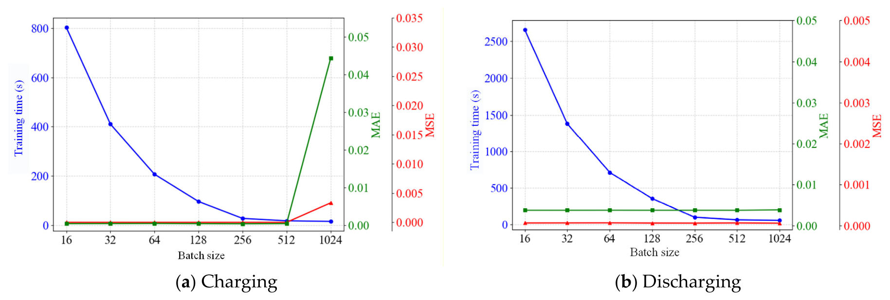
Batch size is a key hyperparameter that affects both model training efficiency and prediction accuracy. To achieve a stable balance between the two, a sensitivity analysis and value calibration of batch size are conducted. Focusing on the two typical operating conditions of charging and discharging, a total of seven batch size values—16, 32, 64, 128, 256, 512, and 1024—are selected, while other parameters such as learning rate, number of iterations, and optimizer type are kept consistent. The MAE, MSE, and training time of the model are compared, and the results are shown in Table 3.
Table 3.
Performance comparison of different batch sizes.
From the perspective of training time, in both charging and discharging scenarios, the training time decreases as the batch size increases, but the reduction rates exhibit noticeable differences. When the batch size increases from 16 to 256, the training time drops significantly. For example, in the charging scenario, when the batch size increases from 16 to 64, the training time is reduced by approximately 70%. However, when the batch size exceeds 256, the rate of decrease in training time gradually slows down. In particular, when the batch size increases from 512 to 1024, the training time reduction in both scenarios is less than 5%, indicating that the marginal benefit of improving training efficiency by increasing the batch size has become extremely low at this point.
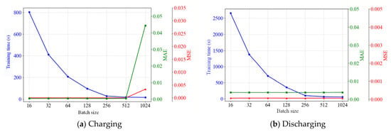
From the perspective of model accuracy, the trends in both scenarios exhibit both similarities and key differences. When the batch size is ≤512, the MAE and MSE in both charging and discharging scenarios remain relatively stable and stay at low levels, indicating that increasing the batch size within this range does not have a significant negative impact on the model’s fitting capability. However, when the batch size is further increased from 512 to 1024, the accuracy metrics in the charging scenario deteriorate significantly: the MSE rises from 0.0042 × 10⁻⁴ to 33.3552 × 10⁻⁴, the MAE increases from 0.48624 × 10⁻³ to 44.29544 × 10⁻³, and R2 drops from 0.999983 to 0.872042, as shown in Figure 13. The core reason is that when the batch size is excessively large, the representativeness of the gradient information from the samples within a single iteration declines, making it difficult for the model to converge to the optimal parameter space.
Figure 13.
Performance of different batch sizes under charging and discharging conditions.
Based on the joint consideration of predictive accuracy and training efficiency, a batch size of 512 was selected as the best compromise for both operating conditions. Although a batch size of 256 yields slightly lower charging MAE and a batch size of 1024 achieves the lowest discharging RMSE, the latter significantly degrades charging prediction accuracy. In contrast, a batch size of 512 maintains stable predictive performance while substantially reducing training time in both scenarios. Therefore, 512 was selected based on the overall trade-off between predictive accuracy and computational efficiency, rather than the optimum of any single metric.
4.3. Multi-Model Comparative Experiment
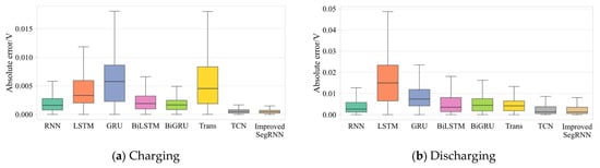
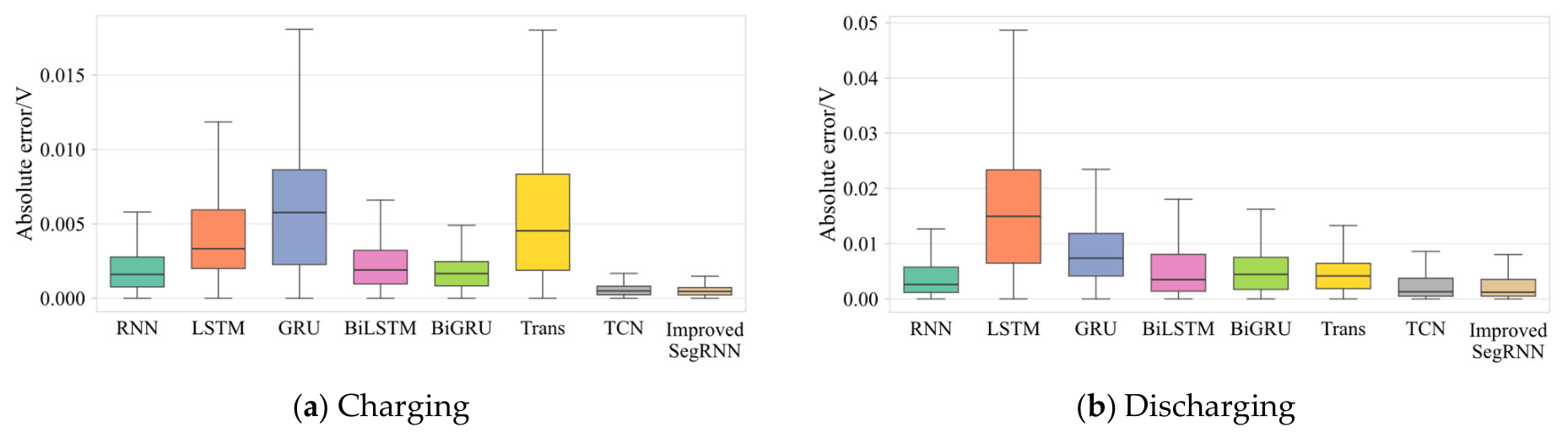
To comprehensively evaluate the prediction capability of the proposed improved SegRNN model under different operating conditions, it is compared with seven baseline methods—RNN, LSTM, GRU, Bi-LSTM, Bi-GRU, Transformer, and TCN—on both charging and discharging tasks. Under charging tasks, the improved SegRNN achieves the lowest RMSE and MAE and the highest R2 among all eight models. Under discharging tasks, TCN achieves a slightly lower RMSE (7.86925 × 10⁻³ vs. 8.2487 × 10⁻³) and a higher R2 (0.998082 vs. 0.997891). However, the improved SegRNN achieves the lowest MAE (3.76869 × 10⁻³) and the shortest training time (66.93 s/epoch) among all eight models. These results indicate that the advantages of the proposed model vary across operating conditions and evaluation metrics. The detailed comparison results are presented in Table 4 and Figure 14.
Table 4.
Performance comparison of different models.
Figure 14.
Box plots of prediction errors for each model under charging and discharging conditions.
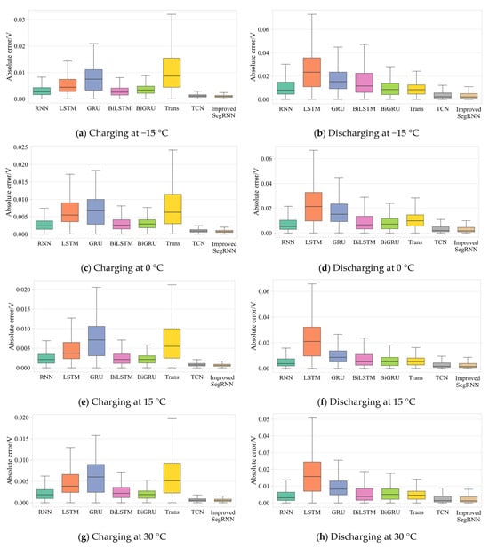
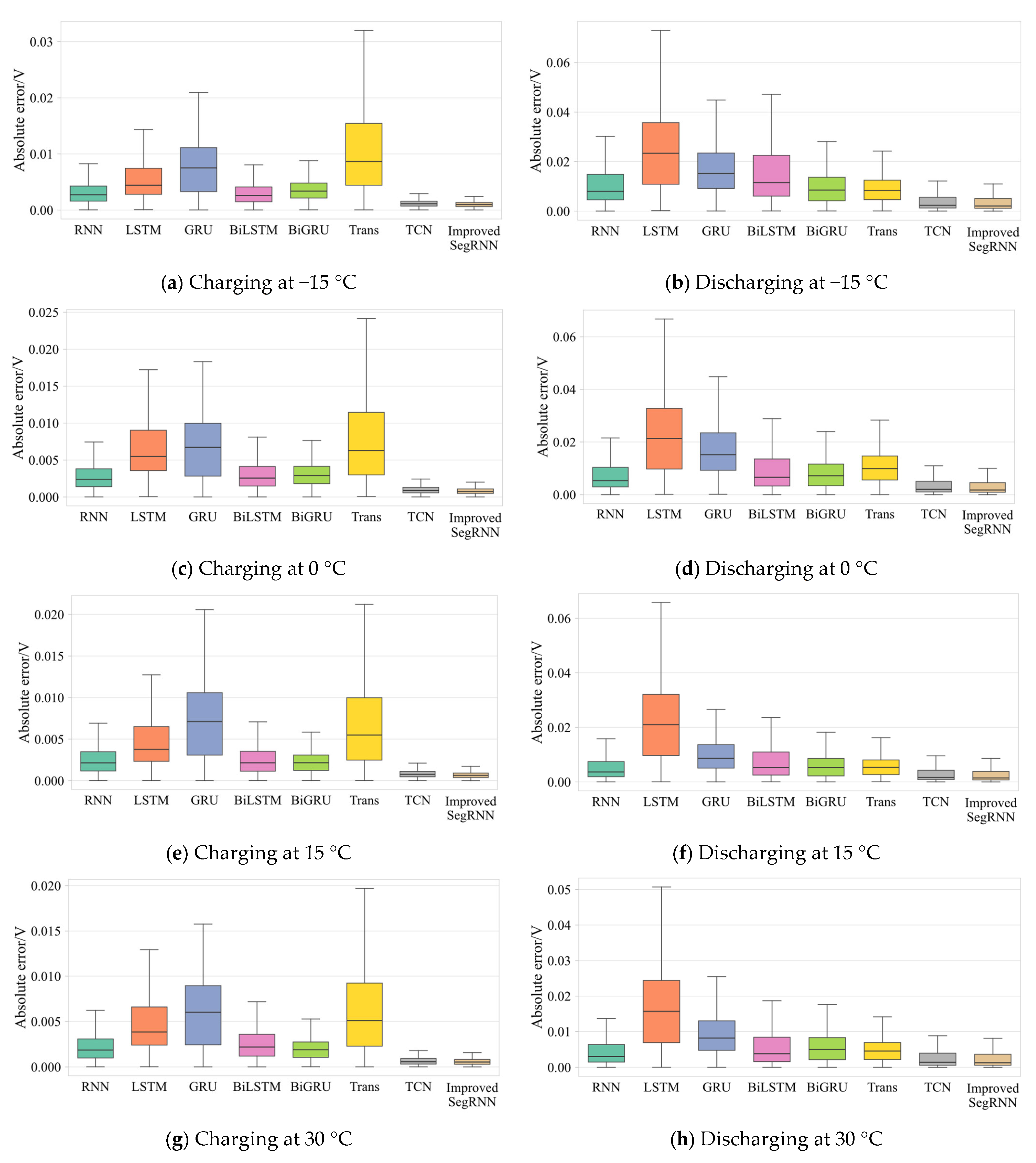
Considering that the geographical distribution of the user base is extensive and the ambient temperature fluctuates significantly with the seasons, the ambient temperature of the on-board lithium-ion power battery varies considerably under different spatiotemporal conditions. This factor may interfere with the prediction accuracy of the thermal runaway warning model. To this end, samples from four typical temperature gradients in the dataset—−15 °C, 0 °C, 15 °C, and 30 °C—are selected to represent different ambient temperature conditions. The experimental results are shown in Figure 15. Therefore, Figure 15 reports the prediction performance of each model under four ambient temperature stratifications, rather than as an assertion of environmental generalization over the entire operating range. Whether the model ranking is maintained outside these four layers has not been evaluated.
Figure 15.
Box plots of prediction errors for each model under charging and discharging at different temperatures.
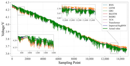
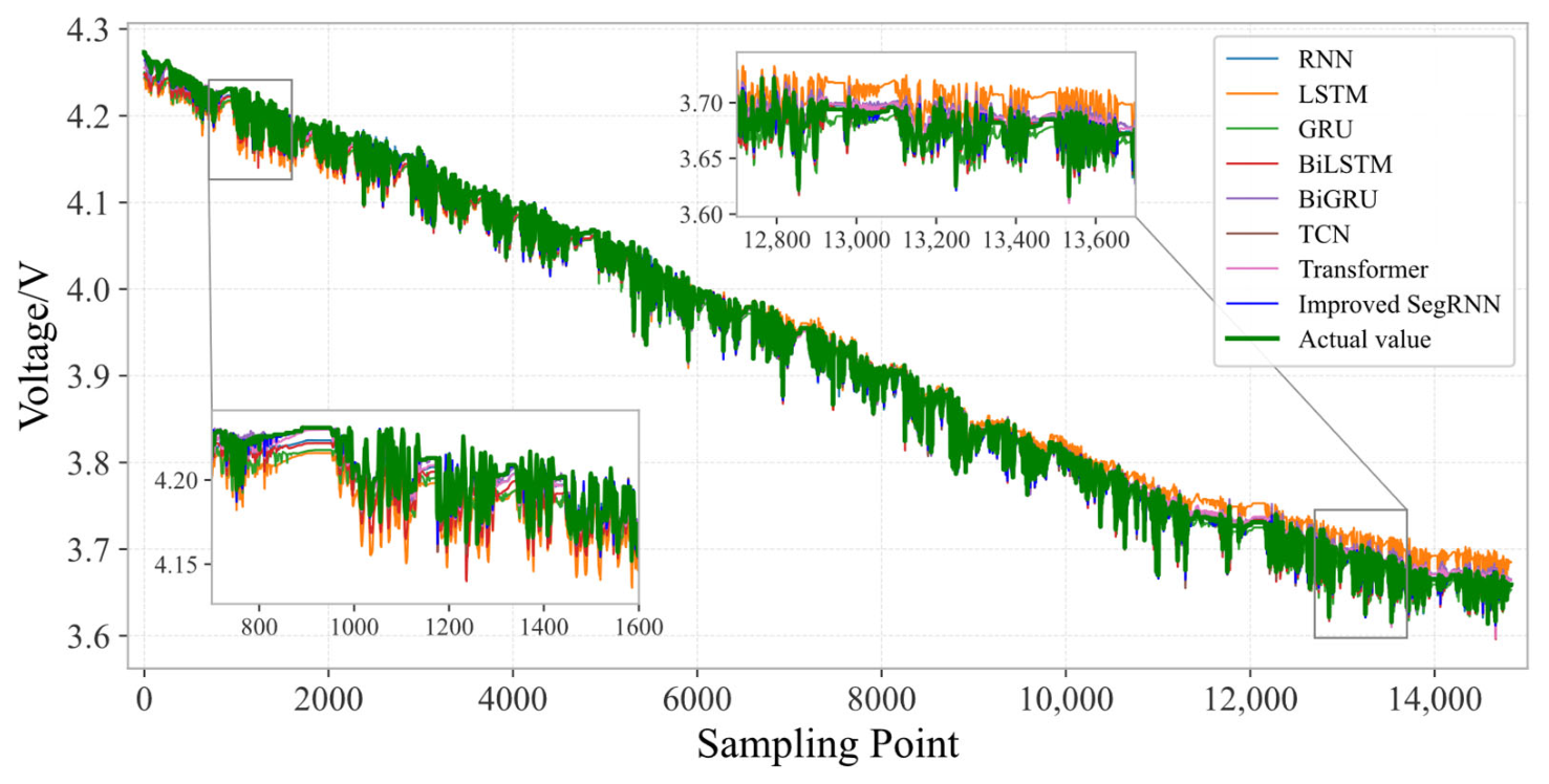
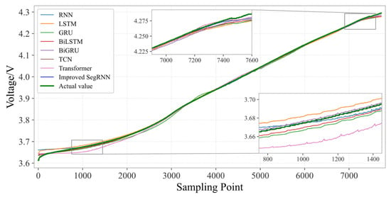
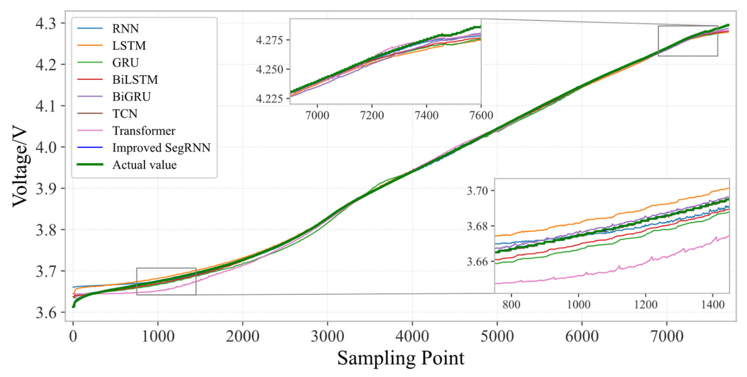
Further, from the perspective of temporal consistency, the comparison results of the median voltage prediction in Figure 16 (discharging state) and Figure 17 (charging state) show that the improved SegRNN model significantly outperforms the compared models, such as LSTM, GRU, Bi-LSTM, and Transformer, in terms of prediction stability and accuracy over the entire cycle.
Figure 16.
Voltage values at each moment during discharging.
Figure 17.
Voltage values at each moment during charging.
From the perspective of the discharging stage, the prediction deviations of traditional models exhibit evident staged characteristics as the state of charge (SOC) varies. In the early discharging stage, the predicted values of the LSTM, GRU, and Bi-LSTM models were approximately 0.02 V lower than the actual values. This deviation stems from these models’ insufficient capture of the rapid voltage variation characteristics at the beginning of discharge, making it difficult to accurately fit the electrochemical properties of the battery during the initial discharging stage. Entering the late discharging stage, as the remaining capacity continues to decrease, the internal polarization effect of the battery intensifies. The prediction deviation of the LSTM model further expands, not only shifting from underestimation to overestimation but also showing an increasing trend as the remaining capacity decreases. Although GRU and Bi-LSTM did not exhibit a reversal in the deviation direction, they still maintained a certain level of error. This is essentially due to the limited learning capability of the RNN structure for long-range dependencies, which prevents it from stably memorizing the voltage variation pattern over the entire discharge cycle of the battery for an extended period.
During the charging stage, the staged deviations of the compared models are equally prominent. In the early charging stage, the LSTM, GRU, and Transformer models exhibit a difference of approximately 0.02 V from the actual values. This is because the battery is in a high-current acceptance state at the beginning of charging, with a rapid voltage rise rate. The attention mechanism of the Transformer tends to over-focus on local features, and the gating structure of the GRU lags in responding to rapidly changing features, leading to deviations in the early-stage predictions. Although the prediction deviations of the models improve as charging progresses, the GRU model still exhibits slight outliers in the late charging stage.
In stark contrast, the proposed improved SegRNN method demonstrates excellent prediction performance throughout the entire charging and discharging cycle. Whether in the charging or discharging stage, its prediction curve always closely follows the actual value changes without producing significant deviations due to variations in the state of charge. The core reason for this advantage lies in the structural improvements of the proposed method, such as segmented time-series modeling, which not only resolves the memory decay problem of traditional RNNs for long-range dependencies but also avoids the feature capture deviations of models such as Transformer and GRU during periods of rapid voltage change or plateau phases. It can accurately adapt to the multi-stage characteristics over the full charging and discharging cycle of the battery, ultimately achieving unbiased prediction across all scenarios. Compared with the systematic deviations exhibited by some baseline models during the rapid-change period in the early discharging stage or the enhanced polarization period in the late discharging stage, the proposed method can maintain a more consistent tracking capability throughout multi-stage dynamic processes, indicating that the segmented recurrence and channel fusion mechanism has a more robust modeling effect under long-sequence and strongly non-stationary conditions.
Taken together, the experiments reported in this chapter support the following interpretation. Under the charging condition, the improved SegRNN is the most accurate of the eight compared models, attaining the lowest RMSE (0.64961 × 10⁻³), the lowest MAE (0.48624 × 10⁻³), the highest R2 (0.999983), and the shortest training time among the seven baseline methods (18.63 s/epoch). Under the discharging condition, the advantage is task-dependent rather than uniform: TCN reaches a slightly lower RMSE (7.86925 × 10⁻³) and a slightly higher R2 (0.998082) than the proposed model, whereas the proposed model retains the lowest MAE (3.76869 × 10⁻³) and the shortest training time among the seven baseline methods (66.93 s/epoch). Combined with the retrospective validation, in which the hierarchical strategy raises the first Level 1 warning on average 87.3 days and the Level 3 warning on average 2.3 days before the recorded thermal runaway event, the results indicate that the proposed architecture is best suited to the charging condition, and that its residual-based warning rule provides a usable lead time on real vehicles.
4.4. Ablation Study
To evaluate the contribution of the improved SegRNN, an ablation study is conducted. The improved SegRNN is compared with a SegRNN. All other experimental settings are kept identical, including the input features, historical window, segment length, hidden dimension, optimizer, learning rate, batch size, early-stopping criteria, and vehicle-level data split. The improved model incorporates a two-layer, four-head cross-variable self-attention module, followed by a one-dimensional convolutional channel-fusion layer. In the ablated model, the original SegRNN architecture is retained. This includes segmented projection, recurrent encoding, and parallel decoding. In addition, the output projection of the attention block and the final feedforward layer are zero-initialized to minimize the initial contribution of the added attention module. The experimental results are presented in Table 5.
Table 5.
Ablation study of the two proposed modules: under the same training settings, the improved SegRNN encoder is compared with the same encoder after removing the fusion of cross-variable self-attention and convolution channels.
The improved SegRNN improves prediction accuracy under both operating conditions. During charging, RMSE decreases from 0.65084 × 10⁻³ to 0.64961 × 10⁻³ (0.19%), while MAE decreases from 0.49256 × 10⁻³ to 0.48624 × 10⁻³ (1.28%). During discharging, RMSE decreases from 8.34603 × 10⁻³ to 8.24870 × 10⁻³ (1.17%), and MAE decreases from 4.02911 × 10⁻³ to 3.76869 × 10⁻³ (6.46%). R2 also increases slightly under both conditions. In addition, the improvement is more pronounced during discharging, particularly in terms of MAE. The relatively small improvement during charging may be attributed to the smoother voltage profiles and the already high prediction accuracy of the baseline model. In contrast, voltage variations during discharging are more strongly influenced by changes in current and driving conditions. The added modules may therefore provide greater benefits in capturing these complex relationships. The improved accuracy comes at the cost of increased model complexity. Although the number of model parameters approximately triples, the training time increases only slightly. During charging, the training time increases from 18.02 to 18.63 s/epoch (3.4%). During discharging, it increases from 65.04 to 66.93 s/epoch (2.9%). The experimental results presented above demonstrate the effectiveness of the improved SegRNN proposed in this study.
5. Conclusions
This study proposes a hierarchical thermal runaway warning method based on an improved SegRNN model for electric vehicles. Separate feature screening is performed for charging and discharging conditions. A cross-variable self-attention module and a one-dimensional convolutional channel fusion layer are integrated into SegRNN to improve cell voltage prediction. A three-level warning strategy is then developed based on voltage prediction residuals. Evaluation using real-world vehicle data demonstrates the effectiveness of the proposed method. Under charging conditions, the proposed model achieves the lowest RMSE (0.64961 × 10⁻³) and MAE (0.48624 × 10⁻³) among all compared models. Under discharging conditions, it achieves the lowest MAE (3.76869 × 10⁻³) and shortest training time (66.93 s/epoch), while maintaining competitive RMSE performance. Retrospective validation on six vehicles with confirmed thermal runaway events shows average warning lead times of 87.3 days for Level 1 and 2.3 days for Level 3. The method also identifies suspected abnormal cells in the evaluated incomplete-data scenarios. These results demonstrate the potential of the proposed method for early risk identification and hierarchical thermal runaway warning.
Several limitations should be acknowledged. The dataset lacks diverse fault scenarios and long-term battery aging records, which may limit model generalizability. In addition, the warning thresholds were determined based on engineering recommendations and validation results, without explicitly modeling the effects of sensor faults, cell inconsistency, and battery aging. This may lead to false alarms under certain operating conditions. Future work will incorporate more diverse datasets, refine the warning thresholds, and improve model generalizability and computational efficiency through cross-vehicle transfer learning and model lightweighting.
Author Contributions
Conceptualization, J.L. and Y.Z.; methodology, D.L.; software, J.L., Y.Z. and D.L.; validation, S.C. and Y.L.; formal analysis, J.L. and Y.Z.; investigation, Y.Z. and D.L.; resources, P.Z., Z.W. and J.H.; data curation, Y.L. and B.Y.; writing—original draft preparation, J.L., Y.Z., D.L. and M.W.; writing—review and editing, J.L., Y.Z., B.Y., X.Z., R.H. and M.W.; visualization, J.L., Y.Z. and P.Z.; supervision, P.Z., Z.W. and J.H.; project administration, J.H.; funding acquisition, R.H. All authors have read and agreed to the published version of the manuscript.
Funding
This research was funded by the Fundamental Research Funds for the Central Universities (Grant No. 104972026RSCbs0118, 104972026KFYd0037). This research was also funded by the Postdoctoral Fellowship Program of the China Postdoctoral Science Foundation under Grant Number GZB20260331.
Data Availability Statement
Dataset available on request from the authors.
Conflicts of Interest
Authors Jing Liu and Min Wei is employed by SAIC GM Wuling Automobile Co., Ltd. The remaining authors declare that the research was conducted in the absence of any commercial or financial relationships that could be construed as a potential conflict of interest.
Abbreviations
The following abbreviations are used in this manuscript:
| BMS | Battery Management System |
| Conv1d | One-Dimensional Convolution |
| DC-DC | Direct Current-Direct Current (Converter) |
| GRU | Gated Recurrent Unit |
| LSTM | Long Short-Term Memory |
| MAE | Mean Absolute Error |
| MSE | Mean Squared Error |
| NEV | New Energy Vehicle |
| ReLU | Rectified Linear Unit |
| RMSE | Root Mean Squared Error |
| RNN | Recurrent Neural Network |
| R2 | Coefficient of Determination |
| SegRNN | Segmented Recurrent Neural Network |
| SOC | State of Charge |
| TCN | Temporal Convolutional Network |
| VIN | Vehicle Identification Number |
References
- Cai, S.; Hu, J.; Chen, J.; Xu, W. Adap-STWT: Real-time traffic flow prediction based on multi-scale graph adaptive fusion and spatio-temporal wavelet transformer. IEEE Trans. Intell. Transp. Syst. 2026, 27, 9022–9035. [Google Scholar] [CrossRef] [Scilit]
- Huang, R.; Wei, G.; Wang, X.; Jiang, B.; Zhu, J.; Chen, J.; Wei, X.; Dai, H. Revealing the low-temperature aging mechanisms of the whole life cycle for lithium-ion batteries (nickel-cobalt-aluminum vs. Graphite). J. Energy Chem. 2025, 106, 31–43. [Google Scholar] [CrossRef] [Scilit]
- Singh, J.; Garg, A.; Kumar, P.; Shakya, R.; Sahu, T.R.; Kumar, A.; Kumar, A.; Shukla, P.K. Thermal–hydraulic performance analysis of micro pin-fin heat sinks with different fin geometries: A numerical study. Heat Transf. 2026, early view. [Google Scholar] [CrossRef] [Scilit]
- Garg, A.; Akkinepally, B.; Harursampath, D.; Shim, J. Empowering urban skies: Energy storage solutions with batteries, fuel cells, and supercapacitors for advanced air mobility and air taxi systems. ChemRxiv 2025. [Google Scholar] [CrossRef] [Scilit]
- Abbas, M.M.; Kwon, B.; Premnath, V.; Jeevarajan, J.; Jain, A. A parametric analysis of thermal runaway and its mitigation in large-scale lithium-ion battery storage scenarios. J. Energy Storage 2026, 167, 122409. [Google Scholar] [CrossRef] [Scilit]
- Gan, Y.; Huang, J.; Gao, W.; Wang, H. Experimental investigation on thermal runaway propagation and gas venting in large-format battery packs: From cell to module. J. Energy Storage 2026, 161, 121952. [Google Scholar] [CrossRef] [Scilit]
- Jin, C.; Feng, X.; Sun, Y.; Lai, X.; Zheng, Y.; Xu, C.; Wan, H.; Wang, L.; He, X.; Ouyang, M. Unplugging the truth: An empirical analysis of 417 fires of electric vehicles and the limitations of battery safety regulations. Energy Storage Mater. 2026, 86, 105035. [Google Scholar] [CrossRef] [Scilit]
- Suddeepong, C.; Nuchkum, S.; Donjaroennon, N.; Leeton, U. A battery management system capable of analyzing abnormal cell trends. Energies 2026, 19, 3062. [Google Scholar] [CrossRef] [Scilit]
- Hong, J.; Zhang, L.; Zhang, C.; Li, M.; Liang, F.; Li, K.; Tang, A.; Chen, Y.; Huang, Z.; Ma, F. Thermal runaway boundary recognition and early detection of lithium battery based on machine vision algorithm. Energy 2025, 340, 139285. [Google Scholar] [CrossRef] [Scilit]
- Wang, J.; Long, T.; Chen, H.; He, C.; Wang, Z.; Jia, Y.; Wang, W.; Wang, H. Thermal runaway characteristics and multi-parameter coupled early warning of large-capacity lithium iron phosphate batteries under external heating. Appl. Therm. Eng. 2026, 300, 131376. [Google Scholar] [CrossRef] [Scilit]
- Emon, M.I.S.; Tam, W.C.; Chen, J.; Fang, H.; Putorti, A. Development of a reliable detection approach for lithium-ion battery thermal runaway using multimodal acoustic-image fusion. J. Power Sources 2026, 685, 240514. [Google Scholar] [CrossRef] [Scilit]
- Cai, S.; Chen, J.; Hu, J.; Huang, R.; Liao, J.; Wei, M.; Zhang, P. HA-LLM: A domain knowledge-enhanced large language model for vehicle-cloud collaborative battery health awareness. Energy Storage Mater. 2026, 86, 104983. [Google Scholar] [CrossRef] [Scilit]
- Dini, P.; Paolini, D. Data-driven analysis and machine learning-based estimation of SOC and RUL in lithium-ion batteries using heterogeneous operational data. Batteries 2026, 12, 199. [Google Scholar] [CrossRef] [Scilit]
- Hammou, A.; Petrone, R.; Diallo, D.; Tala-Ighil, B.; Boussiengue, P.M.; Chaoui, H.; Gualous, H. Machine learning-based lifetime prediction of lithium batteries: A comparative assessment for electric vehicle applications. Energies 2026, 19, 1203. [Google Scholar] [CrossRef] [Scilit]
- Li, Y.; Wang, R.; Jin, Y.; Sun, Z.; Liu, H.; Liu, Y.; Liu, Y.; Xu, J.; Tao, Y.; Jiang, Z.; et al. A novel SOC estimation method for lithium-ion batteries based on serial LSTM-UKF fusion. Energies 2026, 19, 1467. [Google Scholar] [CrossRef] [Scilit]
- de la Vega, J.; Riba, J.R.; Ortega-Redondo, J.A. On the use of machine learning methods for EV battery pack data forecast applied to reconstructed dynamic profiles. Appl. Sci. 2025, 15, 11291. [Google Scholar] [CrossRef] [Scilit]
- Olteanu, M.; Petreuș, D. Predictive active cell balancing for li-ion batteries using GRU-based voltage estimation. Electronics 2026, 15, 1985. [Google Scholar] [CrossRef] [Scilit]
- Xu, Y.; Zhang, X. Electrochemical impedance spectroscopy-driven multi-scale feature fusion and transformer learning for predicting lithium-ion battery lifetime. J. Energy Storage 2026, 164, 121902. [Google Scholar] [CrossRef] [Scilit]
- Guo, L.; He, H.; Ren, Y.; Li, R.; Jiang, B.; Gong, J. Prognostics of lithium-ion batteries health state based on adaptive mode decomposition and long short-term memory neural network. Eng. Appl. Artif. Intell. 2024, 127, 107317. [Google Scholar] [CrossRef] [Scilit]
- Mohamud, N.M.; Ayob, S.M.; Saimon, S.M.; Nahhas, A.M.; Arfeen, Z.A.; Masud, M.I.; Aman, M. Lithium-ion battery state of health prediction using a hybrid BiLSTM–random forest framework. Batteries 2026, 12, 210. [Google Scholar] [CrossRef] [Scilit]
- Hu, J.; Weng, L.; Gao, Z.; Yang, B. State of health estimation and remaining useful life prediction of electric vehicles based on real-world driving and charging data. IEEE Trans. Veh. Technol. 2023, 72, 382–394. [Google Scholar] [CrossRef] [Scilit]
- Song, S.; Zhang, C.; Song, C.; Duan, W.; Xiao, F.; Jin, L.; Qi, C. A deep learning hybrid model for battery state of health estimation based on reconstructed current and voltage vurves. Automot. Innov. 2026, 9, 845–861. [Google Scholar] [CrossRef] [Scilit]
- Zhang, Q.; Zhu, J.; Wang, Y.; Wei, X.; Dai, H. A model cluster adapting to different charge voltage segments for battery capacity estimation. Automot. Innov. 2025, 8, 753–768. [Google Scholar] [CrossRef] [Scilit]
- Chen, Y.; Zhang, S.; Tang, X.; Li, H. Real-world vehicle charging duration prediction based on transfer learning with SENet-CNN-transformer model. Green Energy Intell. Transp. 2025, 5, 100372. [Google Scholar] [CrossRef] [Scilit]
- Meng, Y.; Sun, Q.; Xu, J.; Bian, A.; Yang, Q.; Wang, Z.; Yang, Z.; Zhi, M. Multimodal state of health prediction for lithium-ion batteries via mamba-based fusion of discharge curves and impedance spectra. Batteries 2026, 12, 196. [Google Scholar] [CrossRef] [Scilit]
- Hu, Q.; Wu, M.; Wang, C.; Da, Y.; Du, H. Safety-oriented pre-event severity prediction of lithium-ion battery thermal runaway using interpretable machine learning. Process Saf. Environ. Prot. 2026, 211, 108830. [Google Scholar] [CrossRef] [Scilit]
- Liang, C.; Gao, D.; Cheng, Y.; Yang, Q. Deep learning-based adaptive thermal runaway early warning for electric vehicle lithium-ion batteries during charging and discharging. Comput Chem. Eng. 2026, 213, 109712. [Google Scholar] [CrossRef] [Scilit]



Disclaimer/Publisher’s Note: The statements, opinions and data contained in all publications are solely those of the individual author(s) and contributor(s) and not of MDPI and/or the editor(s). MDPI and/or the editor(s) disclaim responsibility for any injury to people or property resulting from any ideas, methods, instructions or products referred to in the content. |
© 2026 by the authors. Licensee MDPI, Basel, Switzerland. This article is an open access article distributed under the terms and conditions of the Creative Commons Attribution (CC BY) license.