


Abstract
Artificial spin ice provides a versatile platform for investigating geometrical frustration and emergent collective phenomena. However, direct visualization and manipulation of individual magnetic moments remain challenging in conventional nanoscale systems. Macroscopic magneto-mechanical analogs offer an alternative approach by enabling direct observation of individual magnetic elements and flexible control of their interactions. Here, we construct a visible frustrated square lattice composed of mechanically confined permanent magnets and investigate the evolution of collective configurations by varying the intra-unit gap l. We find a non-monotonic order–disorder–order evolution as l is varied. This behavior is associated with the competition between intra-unit and inter-unit magnetic interactions, together with the dissipative and metastable nature of the mechanical system. Vertex statistics, spatial correlations, domain-size distributions, and reciprocal-space magnetic structure factors consistently characterize the evolution of the collective states. Positional-uncertainty analysis further shows that the observed evolution is robust against the experimental positioning accuracy. Our results demonstrate that local interaction engineering provides an effective route for controlling collective states in a macroscopic frustrated magneto-mechanical lattice and establish a directly visible platform for exploring interaction competition and metastability in frustrated systems.
1. Introduction
Geometric frustration [1,2] arises when local interaction energies cannot all be simultaneously minimized, giving rise to competing configurations and collective phenomena. The square-ice model [3,4] is a representative frustrated lattice in which four magnetic elements meet at each vertex and low-energy configurations are commonly classified according to the two-in, two-out ice rule. Artificial spin ice [5,6] based on nanoscale magnetic islands has provided an important experimental platform for studying frustrated configurations and emergent excitations [7,8,9,10,11,12,13,14,15,16,17]. However, the small size and fast dynamics of nanoscale elements can make direct observation of individual configuration changes and their evolution challenging. Macroscopic magneto-mechanical systems provide a complementary approach because individual magnetic elements can be directly visualized and their geometrical arrangement can be controlled experimentally. In such systems, however, mechanical constraints and friction introduce dissipation and may stabilize metastable configurations. This makes it important to distinguish the experimentally observed collective states from equilibrium states of an idealized spin-ice Hamiltonian [18,19,20]. In this work, we construct a macroscopic magneto-mechanical frustrated lattice in which the separation between two magnets within a unit can be systematically varied [21,22,23,24,25,26,27,28,29]. By fixing the vertex gap (d = 1.1 mm) and changing the unit gap l, we tune the relative strength of intra-unit magnetic interactions while preserving the overall lattice geometry.
Our aim is to investigate how local interaction tuning influences the collective configurations reached under a controlled assembly protocol [30,31,32,33,34,35,36,37,38]. We focus on the experimentally observed evolution of vertex populations, spatial correlations, domain sizes, and reciprocal-space magnetic structure factors [6] as a function of l. We use these observables to characterize the geometry-dependent evolution of the mechanically stabilized states.
2. Experimental Methods
2.1. Sample Design and Definition of the Mechanical Unit
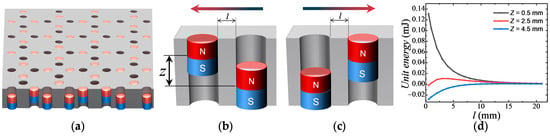
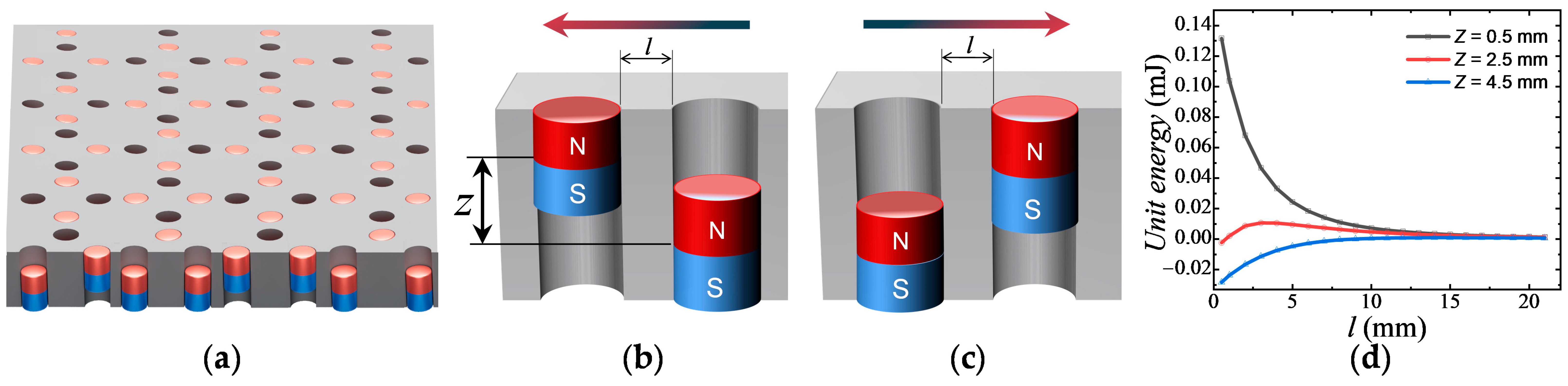
A macroscopic magneto-mechanical system consists of hundreds to thousands of NdFeB magnets arranged in a square lattice on a PMMA plate. Magnets are purchased from Zhanggong District Zhicheng Electronic Products Business Department (Ganzhou city, Jiangxi Province, China). The PMMA plates are purchased from Shanghai Shangjiu Rubber & Plastic Products Co., Ltd. (Shanghai, China). Each magnet is confined in a cylindrical well slightly larger than the magnet diameter, permitting only two vertical states: up or down. The well depth is 10 mm to ensure adequate vertical space. Each unit contains two permanent magnets of different heights (long: 6 mm, short: 5 mm), representing a macroscopic analog of a frustrated magnetic element. The individual magnets possess genuine magnetic dipole moments, but the two-magnet unit is not treated as a physical spin or pseudospin. Instead, we describe each unit using a discrete mechanical state determined by the relative vertical positions of its two magnets. Two low-energy configurations are considered for an isolated unit: (a) left magnet up, right magnet down (left magnetic element) and (b) left long magnet down, right short magnet up (right magnetic element). All magnets are oriented with the North pole up; the long and short magnets are staggered in the lattice. The minimum horizontal spacing within a unit defines the unit gap l (Figure 1b); l values used are 9.7, 2.3, 1.5, 1.1, and 0.7 mm to tune intra-unit magnetic interactions.
Figure 1.
Sample structure and two low-energy configurations of a unit. (a) Schematic of a sample for macroscopic magneto-mechanical systems. Gray, red, and blue denote the PMMA plate, north poles and south poles, respectively. (b) Left-oriented effective unit state. The bold arrow indicates the orientation of the effective dipolar component. The parameter l is the unit gap. Z is the difference between the center heights of the first and second magnets. (c) Right-oriented effective unit state. (d) Variation in unit energy as a function of l for different values of Z.
Each elementary unit consists of two vertically movable permanent magnets confined within a patterned trap. The magnetic moments of the individual magnets are genuine magnetic dipole moments. However, the collective state of a two-magnet unit cannot, in general, be identified with a single spin vector because the net dipole moment of the up–up and down–down configurations along the lattice direction vanishes.
Therefore, rather than assigning a physical spin or pseudospin to each unit, we describe the unit using a discrete mechanical state variable. The four possible configurations are classified as up–up, up–down, down–up, and down–down. The up–down and down–up configurations have a nonzero net dipolar component along the corresponding lattice direction, whereas the up–up and down–down configurations have approximately zero net dipolar moment along that direction and therefore possess a quadrupolar character. This distinction is taken into account when interpreting the magnetic structure factor.
This distinction is important because the mechanical unit is used here as a macroscopic analog of a frustrated magnetic element. In some configurations, an individual magnet may remain at an intermediate vertical position rather than occupying a clearly defined upper or lower state. Such configurations are attributed to mechanical friction and incomplete relaxation during assembly. We refer to them as anomalous magnet configurations or defective unit configurations. They are not interpreted as fractionalized spin states [39,40,41] and are excluded from analyses that require a well-defined binary dipolar state [42,43,44].
The four neighboring units meet at a vertex; the minimum distance between the two adjacent units defines the vertex gap d, fixed at 1.1 mm, enabling analysis of intra-unit vs. vertex interactions. The direction is determined based on the absolute height of the magnets and the relative vertical displacement between the centers of two adjacent magnets. The difference between the center heights of the first and second magnets is denoted as Z. Taking the trap bottom as zero, the height of the magnet top relative to the trap bottom is called the absolute height. When a magnet exhibits the up state, the threshold (minimum) of the absolute height is 9.5 mm; when it exhibits the down state, the threshold (maximum) is 6.5 mm. In principle, a magnet could have an intermediate state, with its absolute height between 4.5 mm and 5.5 mm. Two up magnets form an up-up unit, with Z ranging from −0.5 mm to 0.5 mm. It is represented by two outward arrows. Two down magnets form a down-down unit, with Z ranging from −0.5 mm to 0.5 mm, and it is represented by two inward arrows. Magnets in intermediate states are extremely rare in the square lattice; in such cases, the intermediate-state magnet is represented by an anomalous configuration, marked by two small arrows. At this point, all possible states of a unit have been assigned variables. According to the real parameters, positions and magnetic flux density, the unit energy (interaction energy of two magnets in a unit) can be obtained by COMSOL Multiphysics® v. 6.4 software for different values of Z (Figure 1d).
The positional uncertainty of an individual magnet is approximately 0.05 mm, giving a maximum relative positional uncertainty of approximately ±0.1 mm for a pair of magnets. To assess the influence of this geometric uncertainty, the interaction energies were recalculated for relative positional displacements of +0.1 mm and −0.1 mm. The calculated energies of the relevant vertex configurations change by less than 5%, while their relative trends remain unchanged. Therefore, the observed dependence on l is not explained by the measured positional uncertainty. This geometric uncertainty analysis is distinct from the history dependence associated with friction. Positional uncertainty concerns the accuracy of the assembled geometry, whereas friction determines the dissipative dynamics and may affect which metastable configuration is reached. When intra-unit interaction is strong enough, the unit configurations can exhibit significant changes and influence the vertex types.
2.2. Identification of Vertex Types
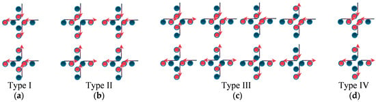
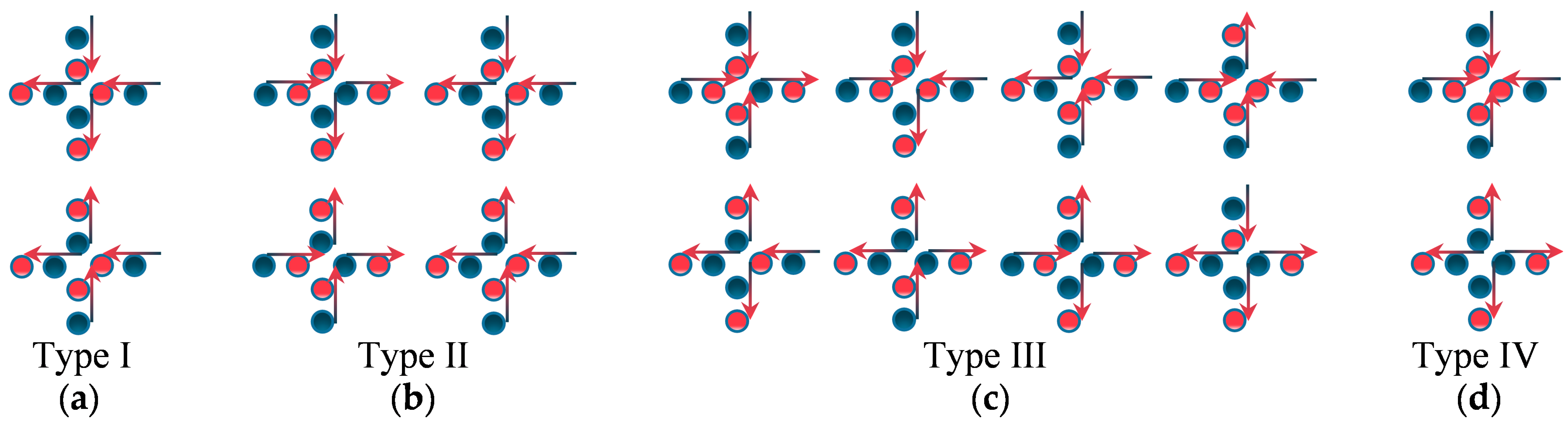
Each vertex is formed by four neighboring magnetic elements. The vertex type is assigned according to the experimentally determined orientation of the magnetic elements surrounding the vertex. Type-I configurations correspond to the lowest-energy vertex configurations in the present geometry (Figure 2a). Type-II configurations satisfy the same ice-rule constraint but have a higher interaction energy (Figure 2b). Type-III configurations violate the two-in/two-out condition and contain an unequal number of elements oriented toward and away from the vertex (Figure 2c). The vertex type of each experimental configuration was determined from the measured magnetic polarity and the vertical state of the corresponding magnets. The classification is applied consistently to all sample geometries.
Figure 2.
Vertex types in macroscopic magneto-mechanical systems. (a) Schematic of Type-I vertices. Vertex gap d is fixed to 1.1 mm. (b) Schematic of Type-II vertices, where units share the same direction for each row and each column. (c) Schematic of Type-III vertices, which are elementary excitations in macroscopic magneto-mechanical systems. (d) Schematic of Type-IV vertices, which rarely appear in the system. Arrows denote orientations of the effective dipolar component. Red and dark blue denote upward and downward states of magnets, respectively.
2.3. Vertex Types and Classification Criteria
At a vertex, four units with unit low-energy states create 16 configurations. Following square ice and artificial spin ice conventions, these configurations are grouped into four classes: Type I (2-in-2-out ice rule; 2 configurations; lowest energy), Type II (2-in-2-out ice rule; 4 configurations; next-lowest energy), Type III (3-in-1-out or 1-in-3-out; 8 configurations; monopole excitations; higher energy), and Type IV (4-in or 4-out; 2 configurations; highest energy; rare; Figure 2d). Type I and II comply with the ice rule; III and IV violate it. The four vertex types are illustrated with dark magnets down and red magnets up; arrows denote orientations of the effective dipolar component (Figure 2). In a fully random array, the proportions are 12.5%, 25%, 50%, and 12.5% for Type I–IV, respectively.
When vertex types include up-up and down-down units, the number of vertex configurations can be expanded to 256, among which there are 32 configurations for Type-I vertices, 64 for Type-II vertices, 128 for Type-III vertices, and 32 for Type-IV vertices. The vertex configuration is mainly determined by the states of the inner four magnets of the vertex, while the outer four magnets of the vertex can be in arbitrary states, thus multiplying the original number of configurations by 16 and generating a large number of new configurations. The correlation U between the two magnets in up-up and down-down units is 1, which does not affect the nearest-neighbor correlation I of the vertex; the nearest-neighbor correlations of Type-I and Type-IV vertices remain −1 and 1, respectively, and those of Type-II and Type-III vertices remain 0. The correlation function L is also unaffected; the L correlations of Type-I, Type-II, Type-III, and Type-IV vertices remain 1, −1, 0, and 1, respectively. Besides affecting the unit correlation function U, up-up and down-down units also change the next-nearest-neighbor correlation L. At this point, the next-nearest-neighbor correlation L cannot be calculated by simple rules and must be analyzed vertex by vertex. In the calculation of the magnetic structure factor, to describe up-up and down-down units and distinguish them from ordinary up-down units, this study uses 11 to represent an up-up unit, 00 to represent a down-down unit, and 01 and 10 to represent different up-down units. The magnet states in each row of horizontal units are represented by binary symbols, with 1 denoting a magnet up and 0 denoting a magnet down. The states of each row of horizontal units are converted into row vectors, and the overall state of the horizontal units is transformed into a matrix. The magnet states in each column of vertical units are also represented by the same binary symbols; then the states of each column of vertical units form a row vector, and the states of all vertical units are transformed into another matrix. These two matrices are then fed into a computer program, which can automatically generate the magnetic structure factor. The magnetic structure factor is computed according to the real positions of magnets.
2.4. Assembly Protocol and Reproducibility
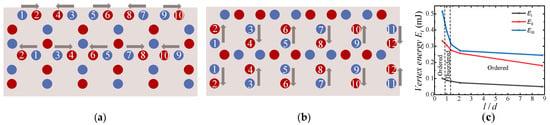
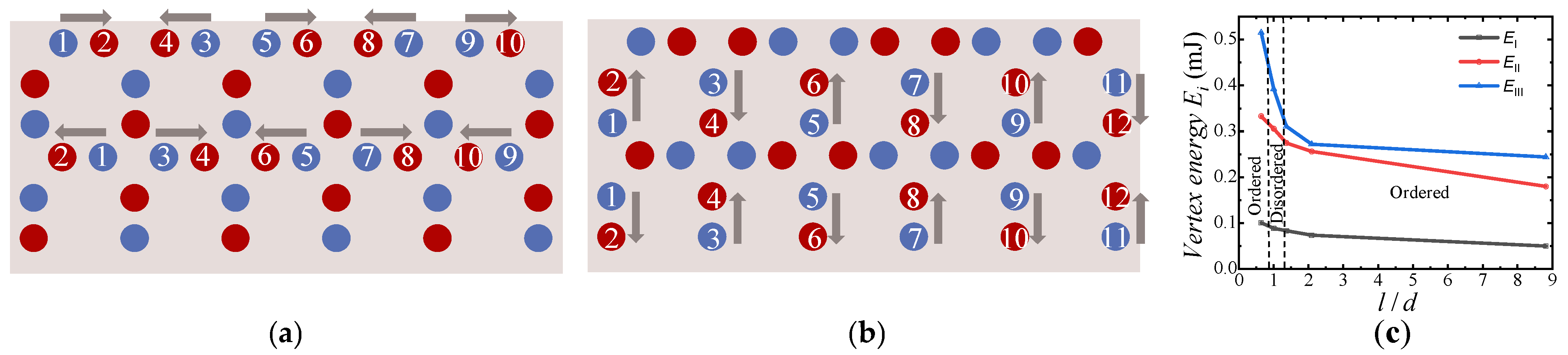
To control variables, the magnets were manually assembled by placing individual magnets into the predefined cylindrical wells of all samples under a controlled assembly protocol. The same assembly protocol was used for all values of l to minimize variations associated with preparation history. Because the magnets are mechanically stabilized by friction, the final configurations may depend on the assembly process and are therefore treated as metastable configurations. In the PMMA base, horizontal unit rows are filled with magnets in a sequence as shown in Figure 3a; neighboring units have opposite magnet order, and adjacent rows have opposite horizontal order. Vertical units follow a similar scheme (Figure 3b). This assembly tends to promote Type-I vertices and enhances near-neighbor interactions, while stronger intra-unit interactions may induce Type-II and Type-III vertices spontaneously. Vertex energy is shown in Figure 3c. The present study does not establish complete ergodicity. Instead, the comparison between different values of l is performed under the same assembly protocol, allowing the geometry-dependent evolution of the experimentally obtained configurations to be systematically investigated. Experiments involving alternative assembly sequences and mechanical annealing would provide an important future test of the dependence on initial conditions.
Figure 3.
Sample assembly protocol in macroscopic magneto-mechanical systems. (a) Magnet order of horizontal units. (b) Magnet order of vertical units. (c) Vertex energy for three types of vertices. Arrows indicate the direction of movement. Numbers in each row indicate the magnet placement order. Gray, red, and blue denote the PMMA plate, short magnets (5 mm in height), and long magnets (6 mm in height), respectively.
To quantitatively characterize the degree to which the system satisfies the ice rule, this work defines two derived physical quantities: (1) the ice-rule satisfaction rate Rice = (NI + NII)/Ntotal, which equals the sum of the proportions of Type-I and Type-II vertices, reflecting the overall proportion of vertices satisfying the ice rule and (2) the monopole excitation density ρmono = (NIII + 2NIV)/Ntotal, reflecting the proportion of vertices that break the ice rule, where NI, NII, NIII, and NIV denote the numbers of the corresponding vertex types, and Ntotal is the total number of vertices. Since Type-IV vertices are rare, the monopole excitation density is approximately equal to the proportion of Type-III vertices.
2.5. Experimental Parameter Characterization
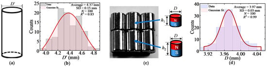
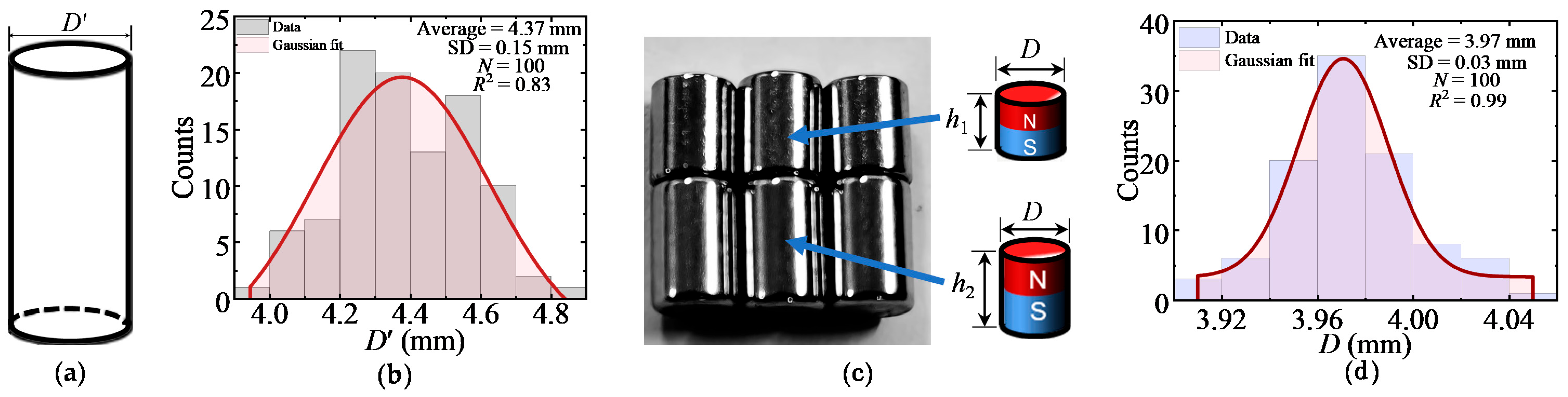
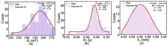
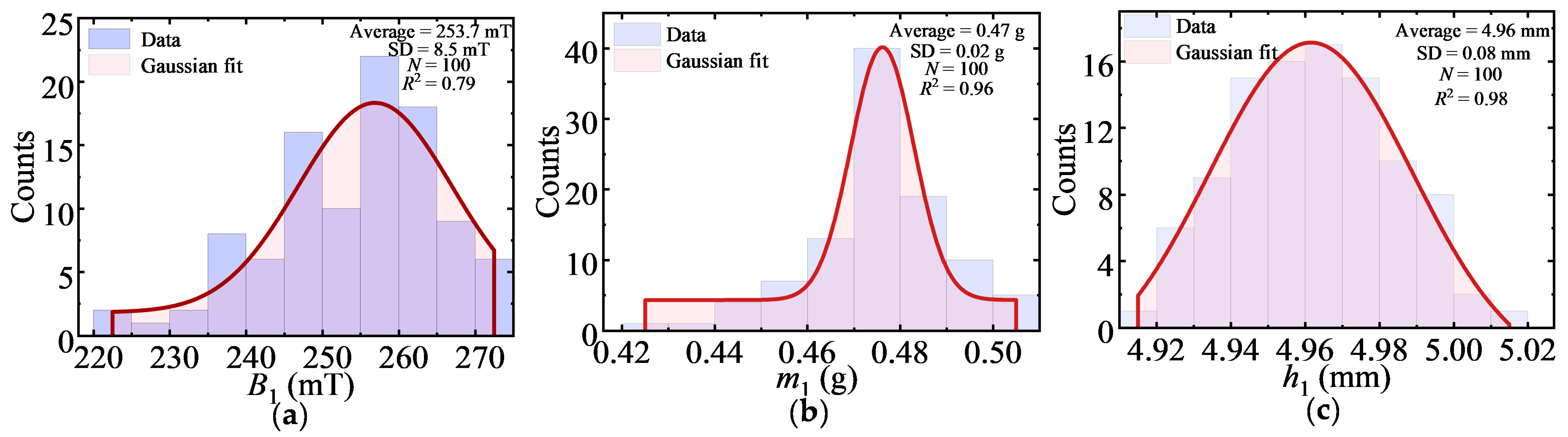
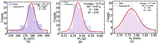
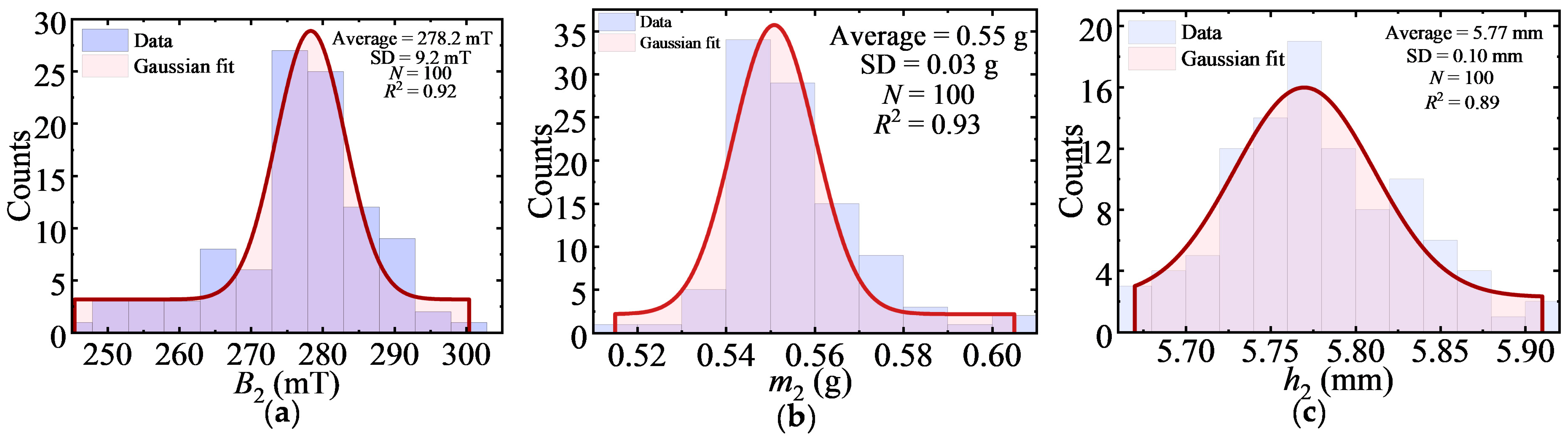
To support the consistency of sample preparation, this study systematically measured and statistically analyzed the key geometric and magnetic parameters of the traps and magnets used in the experiments. As shown in Figure 4a, the key geometric parameter of the trap is the trap diameter D′. The distribution of the trap diameter D′ is shown in Figure 4b. One hundred traps were randomly selected for measurement; their diameters range from 3.88 to 4.88 mm, with a mean value of 4.37 mm and a standard deviation of 0.15 mm, approximately following a Gaussian distribution. Optical images and schematic diagrams of the two types of magnets are shown in Figure 4c. Both types of magnets have the same diameter D, whose distribution is shown in Figure 4d, with a mean value of 3.97 mm and a standard deviation of 0.03 mm. Their heights are denoted as h1 and h2. The magnetic flux densities and masses are denoted as B1, B2, m1, and m2, respectively.
Figure 4.
Traps structures and magnets used in macroscopic magneto-mechanical systems. (a) Trap diameter D′. (b) Distribution of trap diameter D′. (c) Magnets with two different heights. (d) Distribution of magnet diameter D. The red curves in the histogram denotes the Gaussian fit to the data distributions of the corresponding diameters.
One hundred short magnets and one hundred long magnets were selected, and their magnetic flux densities, masses, and heights were measured individually. The measurement results are shown in Figure 5 and Figure 6 and in Table 1 and Table 2. The mean values and standard deviations of each parameter are given in the second and third rows of Table 1 and Table 2, respectively. Gaussian fitting (red curves) shows that all parameters approximately follow Gaussian distributions, indicating good consistency of the magnets. The mean values of the magnetic flux density B1, mass m1, and height h1 of the short magnets are 253.7 mT, 0.47 g, and 4.96 mm, respectively; the corresponding values for the long magnets are 278.2 mT, 0.55 g, and 5.77 mm. The actual heights of the two types of magnets are in good agreement with the design values (5 mm and 6 mm).
Figure 5.
Distributions of measured parameters for short magnets. (a) Distribution of magnetic flux density B1. (b) Distribution of mass m1. (c) Distribution of height h1. The red curves in the histogram denotes the Gaussian fit to the data distributions of the corresponding physical quantities.
Figure 6.
Distributions of measured parameters for long magnets. (a) Distribution of magnetic flux density B2. (b) Distribution of mass m2. (c) Distribution of height h2. The red curves in the histogram denotes the Gaussian fit to the data distributions of the corresponding physical quantities.
Table 1.
Parameters of traps and short magnets.
Table 2.
Parameters of long magnets.
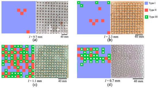
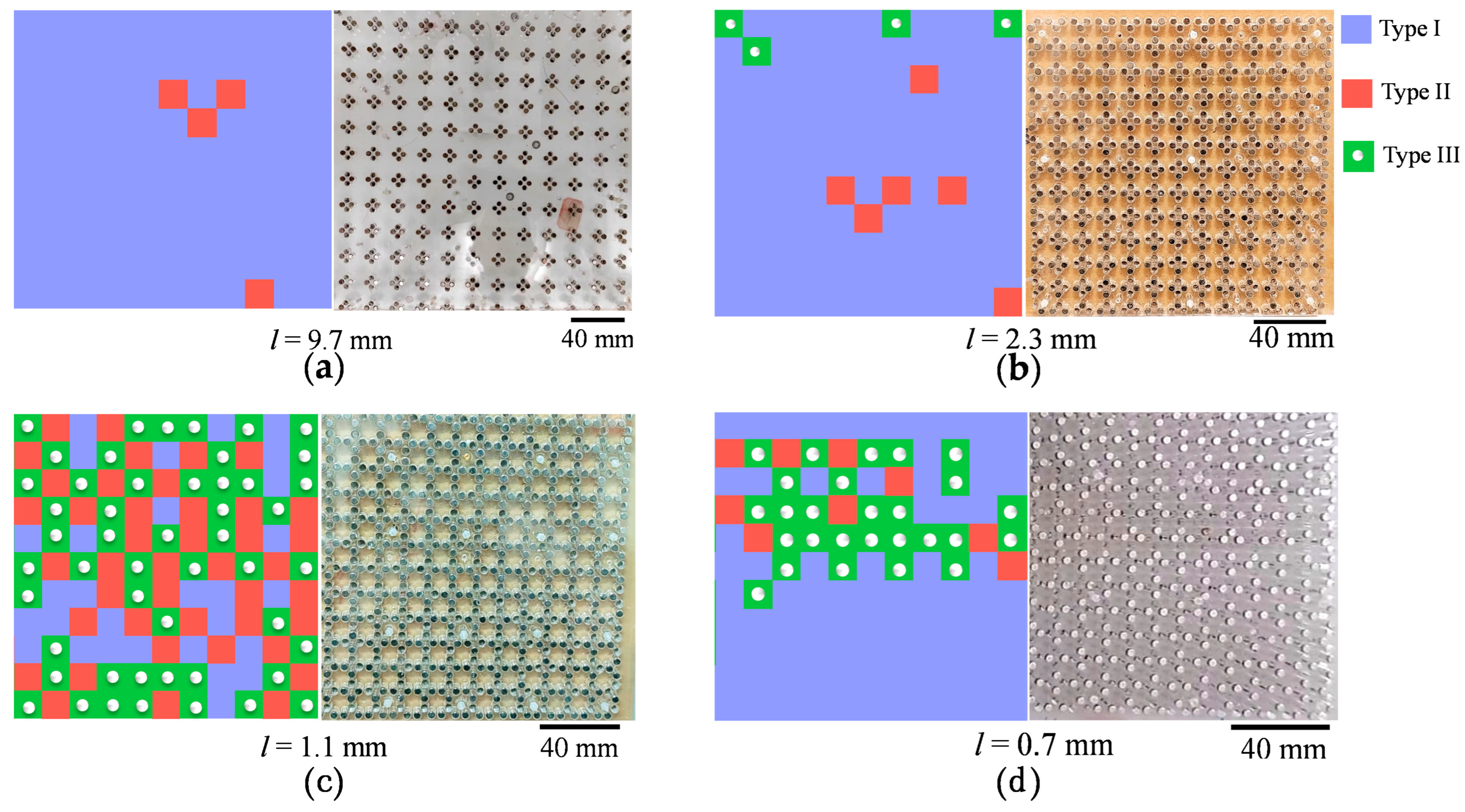
For ease of description, this study classifies the system configurations into three categories based on the characteristic features of the magnetic structure factor: configurations in which bow-tie diffuse characteristic features occur are called excited ordered configurations (EO, Figure 7a); configurations in which the magnetic structure factor shows only antiferromagnetic Bragg peaks are called antiferromagnetic correlated configurations (AFM, Figure 7b); configurations in which antiferromagnetic and ferromagnetic Bragg peaks coexist are called disordered configurations (DC, Figure 7c). It should be noted that the term “configuration” here is used only to describe the experimentally observed orderliness, and correspond to a metastable configuration.
Figure 7.
Representative collective configurations of the macroscopic magneto-mechanical frustrated square lattice. (a) Excited ordered configuration. (b) Antiferromagnetically correlated configuration. (c) Disordered configuration. (d) Antiferromagnetically correlated configuration after further reduction in l.
3. Results
3.1. Vertex Proportions and Evolution of Order
Because the magnets are mechanically confined and stabilized by friction, the present system is dissipative and does not necessarily sample all configurations according to a thermal equilibrium distribution. The final configuration may therefore depend to some extent on the assembly history and should be regarded as a mechanically stabilized metastable configuration. The purpose of the present experiment is consequently to investigate how changing the relative strength of local magnetic interactions affects the collective configurations reached under a controlled assembly protocol. The reproducibility of the observed evolution is evaluated by maintaining the same assembly protocol and by analyzing the effects of positional uncertainty. Future experiments involving systematic variation in assembly protocols and mechanical annealing will be required to determine the metastable state of the system.
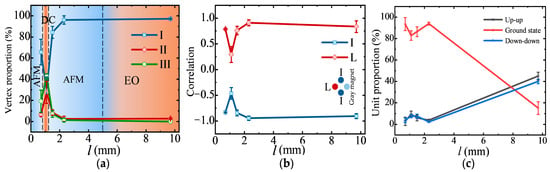
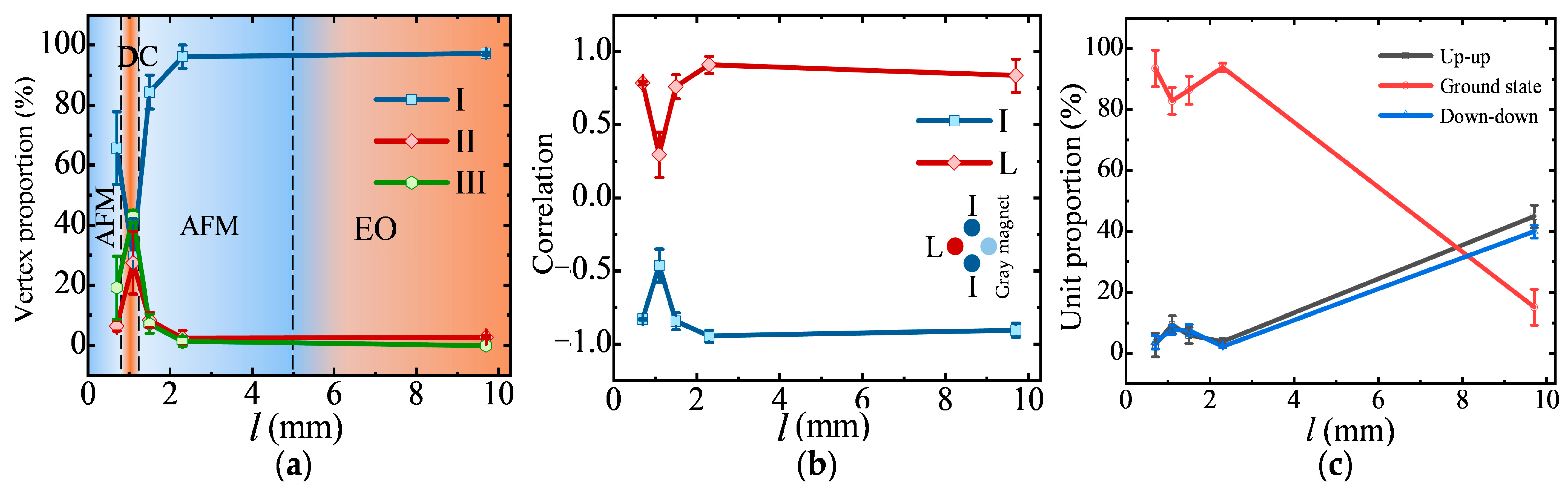
Figure 8a shows the proportions of Type-I, Type-II, and Type-III vertices as a function of the unit gap l. As l decreases from 9.7 mm to 0.7 mm, the vertex populations exhibit a pronounced non-monotonic evolution. At l = 9.7 mm (l ≈ 9d), Type-I vertices account for 97.22% of the vertices, while Type-II and Type-III vertices are present only in small proportions. Although most vertices satisfy the ice-rule condition used for the present classification, many two-magnet units remain in up–up or down–down configurations. We therefore characterize this configuration as an excited ordered configuration, referring to its pronounced real-space spatial organization rather than to a thermodynamically ordered phase. At l = 2.3 mm (l ≈ 2.1d) and 1.5 mm (l ≈ 1.4d), Type-I vertices remain dominant, and the population of anomalous configurations decreases. The resulting configurations exhibit pronounced antiferromagnetic spatial correlations. When l = 1.1 mm (l ≈ d), the Type-I fraction decreases to 36.36%, whereas Type-II and Type-III vertices jump to 24.52% and 39.12%, respectively. The simultaneous increase in these higher-energy vertex configurations corresponds to a strongly disordered collective configuration. When l is further reduced to 0.7 mm (l ≈ 0.64d), the Type-I fraction increases again to 78.79%, accompanied by a reduction in Type-II and Type-III populations. Antiferromagnetic correlations are therefore partially recovered. This sequence is referred to as a non-monotonic order–disorder–order evolution.
Figure 8.
Geometry-dependent evolution of vertex populations and spatial correlations in macroscopic magneto-mechanical systems. (a) States and vertex proportions. Light red, dark red, and blue represent the excited ordered configuration (EO), disordered configuration (DC), and antiferromagnetic correlation configuration (AFM), respectively. (b) Correlation functions of nearest-neighbor I and the next-nearest-neighbor L of a gray magnet. (c) Unit proportions for different types of units.
This can be attributed to the intra-unit magnetic interaction and vertex interaction. For the first row of horizontal units, all magnets are down because the intra-unit magnetic interaction is too weak to overcome the gravitational weight of the magnets. The next row of vertical units will be in the ground state because the upper half of the magnets is stabilized by vertex interactions to be up while the lower half is governed by gravity, resulting in a downward alignment. For the remaining horizontal units, the vast majority of macroscopic magnets are supported by vertex interactions and thus align upward, with only a small number at the boundaries deviating from this state. For the remaining vertical units, the magnets are simultaneously influenced by gravity and the downward repulsive vertex interaction exerted by the horizontal-unit magnets; consequently, except for a few boundary magnets, all are aligned downward. The system is highly ordered with many up-up units and down-down units, so this configuration is called an “excited ordered configuration (EO)”.
As l decreases to 1.5 mm (about 1.4d), the proportion of Type-I vertices drops to 84.35%, while the proportions of Type-II and Type-III vertices rise slowly. At this point, the intra-unit interaction has become strong enough to stabilize most units in their ground states, and the system reaches its ground-state configurations at both the vertex and unit levels, thereby establishing antiferromagnetic ordered configurations. At this point, the proportions of both Type-I and Type-II vertices are below 50%; the ice-rule satisfaction rate (I + II) is only 55.62%, indicating that the system has entered a highly disordered state with a high monopole density. This state arises because the intra-unit interaction and the inter-vertex magnetic interaction become comparable in strength; the friction between the first magnet of a unit and the trap wall is large enough to overcome gravity and keep it in the up state, while the second magnet is down, causing the direction of the unit to reverse. This process is called unit flipping. One unit flip can turn a Type-I vertex into a Type-III vertex, while two unit flips turn it into a Type-II vertex; therefore, the proportion of Type-III vertices is usually higher than that of Type-II vertices, which is consistent with the experimental results. When l decreases from 1.5 mm to 1.1 mm, a macroscopic magneto-mechanical system evolves from an antiferromagnetic configuration to a disordered configuration; when l decreases from 1.1 mm to 0.7 mm, it returns from the disordered configuration to the antiferromagnetic configuration.
When l decreases to 0.7 mm (0.64d), the proportion of Type-III vertices drops to 15.15%, and the ice-rule satisfaction rate recovers to 73.37%, with antiferromagnetic correlation partially restored. From an energy perspective, Type-I vertices have the lowest interaction energy, so when only one type of interaction is present, the system preferentially forms Type-I vertices. However, the system involves competition of interactions. Therefore, as l decreases, the system undergoes a non-monotonic evolution. For l = 9.7, 2.3, 1.5, 1.1, and 0.7 mm, three samples were measured for each value of l. Repeated experiments show that the standard deviations of vertex proportions are all below 13%. With the number of vertices fixed to be 121, non-monotonic evolution occurs in representative samples. For the proportion of Type-I vertices, the largest standard deviation, 12.83%, occurs at l = 1.1 mm and the least standard deviation, 3.91%, occurs at l = 2.3 mm (Table 3). For the proportion of Type-II vertices, the largest standard deviation, 9.29%, also occurs at l = 1.1 mm, but the least standard deviation, 0.95%, occurs at l = 0.7 mm (Table 4). For the proportion of Type-III vertices, the largest standard deviation, 9.02%, occurs at l = 0.7 mm and the least, 1.52%, occurs at l = 9.7 mm (Table 5).
Table 3.
Statistics of Type-I vertices.
Table 4.
Statistics of Type-II vertices.
Table 5.
Statistics of Type-III vertices.
The non-monotonic evolution is consistent with a competition between intra-unit and inter-unit magnetic interactions. At large l, the intra-unit interaction is relatively weak, whereas interactions between neighboring units contribute strongly to the spatial organization of the lattice. As l decreases, the intra-unit interaction becomes increasingly important and modifies the relative energetic preference of different local configurations. Around l ~ d, the competing interactions are sufficiently comparable to produce a broad set of accessible configurations, while friction can stabilize different configurations and prevent complete relaxation. At smaller l, the stronger intra-unit interaction favors a different local arrangement and the observed antiferromagnetic correlations recover. Thus, the observed non-monotonic evolution is consistent with interaction competition, but the present experiment does not by itself establish an equilibrium phase transition.
3.2. Spatial Correlations and Domain Sizes
The changes in correlation functions further support the above evolution trend. The spatial correlation functions provide an independent characterization of the collective-state evolution identified from the vertex populations in Section 3.1. Figure 8b shows the nearest-neighbor correlation I and next-nearest-neighbor correlation L as functions of l. The correlation strengths vary systematically with l, with a pronounced reduction near l = d, where the Type-I fraction reaches its minimum. This reduction indicates weakened spatial coherence and is consistent with the strongly disordered state identified from the vertex statistics. The domain-size distributions provide further evidence for this evolution. At l = 9.7 mm, large Type-I domains dominate the configuration (Table 6). At l = 1.1 mm, the Type-I domains become substantially smaller, while Type-II and Type-III configurations become more prevalent. When l = 0.7 mm, the Type-I domains increase again, consistent with the partial recovery of antiferromagnetic spatial correlations (Table 7). Together, the vertex populations, correlation functions, and domain-size distributions provide mutually consistent real-space signatures of the non-monotonic collective-state evolution.
Table 6.
Maximal size (number of vertices) of a single domain.
Table 7.
Distribution of Type-I magnetic domain sizes and the mean domain size.
When the two magnets have equal lengths, the magnets with flush tops have horizontal interactions, which tend to form excited states. To minimize the occurrence of excited states, this work adopts magnets of different lengths. When the magnet tops are flush, the interactions along the vertical direction between magnets can reduce excited states. The up and down states of the magnets correspond to the north and south poles of ferromagnetic nanoislands, respectively. To avoid a significant difference in magnetic flux density at the two ends of a unit, the length difference between the long and short magnets is only 1 mm. The interaction energy of a unit depends only on the relative vertical displacement between the centers of the two magnets; the vertical displacement, mass, and magnetic flux density between the long and short magnets do not break the energy degeneracy of the two directions. Odd numbers represent short magnets, marked in blue, and even numbers represent long magnets, marked in red. In horizontal units of odd-numbered rows, the magnet order follows a 1243 cycle; in even-numbered rows, the corresponding two units show a 2134 cycle. For vertical units, from the first column to the last column, the magnet order of every two units in odd-numbered columns follows a 2134 cycle, while that in even-numbered columns follows a 1243 cycle. For horizontal units in adjacent rows, the magnet orders are opposite. For vertical units in adjacent columns, the magnet orders are also opposite. At the boundaries, the magnet orders of the first row of horizontal units and the first column of vertical units are given, while those of the last row of horizontal units and the last column of vertical units should be determined according to the parity of the row and column numbers.
An energy competition model can qualitatively explain this phenomenon. Vertex proportions are related not only to the interaction energy but also to the controlled assembly protocol. Because magnets interact with each other during the process, which is similar to the mutual collisions of microscopic molecules, the effect of the controlled assembly protocol can be attributed to a conservative potential-energy barrier. The conservative potential-energy barrier is related to the number of unit flips. The energy landscape of the system should be distinguished from the dissipative mechanical resistance.
The magnetic dipole–dipole interactions and gravitational contribution determine the conservative potential-energy landscape (Epot = Emag + Egrav) of the system. In contrast, friction is a non-conservative dissipative force (Ffriction) that resists magnet motion and can prevent evolution between mechanically accessible configurations. Therefore, the conservative potential-energy difference between two configurations (conservative potential-energy barrier) should not be confused with the dissipative resistance associated with friction. In the present system, friction can stabilize configurations that are not necessarily the lowest-energy configurations during the assembly and relaxation process. The experimentally observed final states should therefore be regarded as mechanically stabilized metastable configurations. The calculated magnetic interaction energies are used to compare the relative energetic preference of different configurations, rather than to claim that the measured states represent thermodynamic equilibrium.
Because friction is history-dependent, the final configuration cannot be assumed to represent a unique metastable state solely from the calculated magnetic energy. Instead, friction mechanically stabilizes configurations that may be metastable. The experimental assembly protocol was therefore kept identical for all values of l to minimize protocol-dependent variations when comparing different geometries.
Under a controlled assembly protocol, the fewer the unit flips required for a vertex, the lower its conservative potential-energy barrier. Type-II vertices require more unit flips than Type-III vertices, so the conservative potential-energy barrier of Type-II vertices is higher than that of Type-III vertices, and the proportion of Type-III vertices is generally higher than that of Type-II vertices. As shown in Table 8 and Table 9, Type-II domains are generally smaller than Type-III domains. Since Type-III vertices can be regarded as elementary excitations, macroscopic magneto-mechanical systems provide new macroscopic experimental evidence for studying elementary excitations in frustrated systems.
Table 8.
Distribution of Type-II magnetic domain sizes and the mean domain size.
Table 9.
Distribution of Type-III magnetic domain sizes and the mean domain size.
3.3. Magnetic Structure Factor
In addition to real-space vertex statistics and spatial correlations, the reciprocal-space magnetic structure factor can also effectively characterize the magnetic order of the system. The magnetic structure factor can provide information about the spatial organization of the magnetic elements. For l = 2.3, 1.5, 1.1, and 0.7 mm, the proportion of the ground state of units is over 80%. Most units can be regarded as Ising spins according to the real positions of magnets. Following the conventional calculation method for the magnetic structure factor in artificial spin ice, the magnetic structure factor I(q) of a macroscopic magneto-mechanical system is defined as follows. Let Si be the direction of the i-th unit, ri be the position of the i-th unit, q be the reciprocal lattice vector, and N be the total number of units. In the present analysis, the magnetic structure factor I(q) is defined from the effective dipolar component of each two-magnet unit. For configurations in which a unit possesses a well-defined nonzero effective dipolar component, the magnetic structure factor is calculated as
where Si represents the effective dipolar component assigned to unit i, ri is its position, and N is the number of units included in the analysis. Here, Si is used as a state variable describing the effective dipolar component and should not be interpreted as a microscopic spin vector. q is the scattering vector. ⟨⋯⟩ denotes the average over the experimentally sampled configurations or spatial correlations included in the analysis. When q = 0, I(0) can be expressed as
I(q) = (1/N)∑i,j eiq·(ri−rj) ⟨Si·Sj⟩
I(0) = (1/N)∑i,j⟨Si·Sj⟩ = (1/N) ⟨(∑iSi)2⟩
The calculation method of the magnetic structure factor is given by Equations (1) and (2), and the results are shown in Figure 9, reflecting the evolution of system order from the reciprocal-space perspective.
Figure 9.
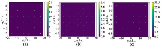
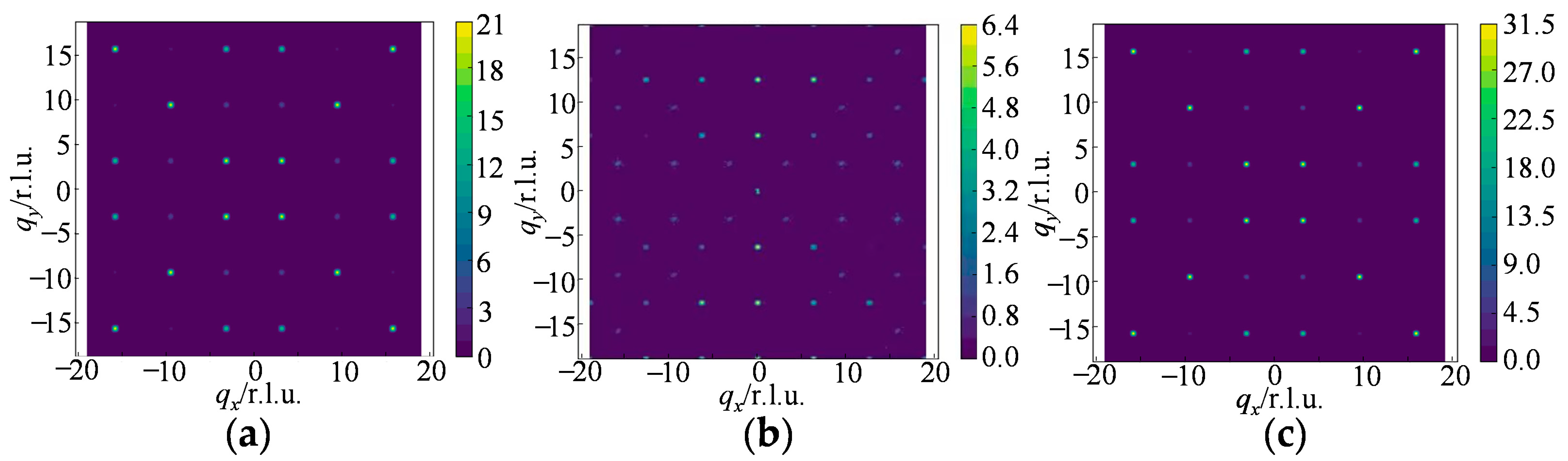
Magnetic structure factors of macroscopic magneto-mechanical systems. (a) Antiferromagnetically correlated configuration for l = 2.3 mm. (b) Disordered configuration for l = 1.1 mm. (c) Antiferromagnetically correlated configurations for l = 0.7 mm. The magnetic structure factor is calculated using the effective dipolar component of the units for which this representation is well defined.
For l = 9.7 mm, a large fraction of the units are in up–up or down–down configurations. These configurations have approximately zero net dipolar moment along the corresponding lattice direction and therefore cannot be adequately represented by the dipolar magnetic structure-factor definition above. A quadrupolar magnetic structure factor could in principle be constructed using the quadrupole moment of each unit, but this requires a different formalism and is beyond the scope of the present analysis. Therefore, the l = 9.7 mm configuration is characterized primarily using the real-space vertex statistics, spatial correlations, and domain-size distributions rather than the present dipolar magnetic structure factor.
At l = 2.3 mm and 1.5 mm, pronounced antiferromagnetic peaks appear in reciprocal space, consistent with the strong antiferromagnetic spatial correlations observed in real space (Figure 9a). At l = 1.1 mm, these peaks become less pronounced, and the reciprocal-space intensity becomes more diffuse, consistent with the disordered state (Figure 9b). At l = 0.7 mm, pronounced antiferromagnetic features re-emerge, indicating partial recovery of spatial order (Figure 9c).
4. Discussion
The results demonstrate a pronounced non-monotonic evolution of the collective configurations [45,46,47,48,49,50,51,52] as the unit gap l is varied. This evolution is consistently reflected in the vertex populations, spatial correlations, domain-size distributions, and reciprocal-space characteristics. The most disordered configuration occurs near l ~ d, where the relative strengths of intra-unit and inter-unit interactions become comparable and the Type-I vertex fraction reaches its minimum. The observed behavior can be interpreted in terms of competing interaction scales. At large l, the intra-unit magnetic interaction is relatively weak, whereas interactions between neighboring units contribute strongly to the spatial organization of the lattice. Reducing l increases the intra-unit interaction and changes the relative energetic preference of the accessible configurations. When the competing interactions become comparable, the system exhibits enhanced configurational disorder. Further reduction in l increases the relative importance of the intra-unit interaction and is accompanied by the recovery of antiferromagnetic spatial correlations.
An important characteristic of the present macroscopic system is its dissipative mechanical nature. Friction is required to mechanically stabilize individual magnets but also prevents the system from freely exploring all configurations. Consequently, the experimentally observed configurations should be regarded as metastable states reached under a controlled assembly protocol. The present experiments, therefore, do not establish thermodynamic ergodicity or a true equilibrium phase transition. Instead, they demonstrate a reproducible geometry-dependent evolution of collective states under the experimental preparation conditions. The positional-uncertainty analysis further shows that the observed non-monotonic behavior is robust against the measured geometric uncertainty. A relative positional displacement of up to approximately ±0.1 mm changes the calculated interaction energies by less than 5% and does not alter their qualitative trends. This supports the interpretation that the observed evolution is not simply a consequence of the positional accuracy of the assembled lattice.
The macroscopic nature of the system provides a practical advantage by allowing individual magnetic elements and their configurations to be directly visualized. This makes it possible to connect local vertex configurations with collective spatial correlations in real space. Future experiments using different assembly sequences, controlled mechanical annealing, and quantitative relaxation measurements will be necessary to determine the extent of history dependence and to establish whether equilibrium behavior can be accessed.
5. Conclusions
We have developed a visible macroscopic magneto-mechanical frustrated lattice in which the relative strength of local magnetic interactions can be tuned through the unit gap l. By systematically varying l while keeping the vertex gap d fixed, we observe a non-monotonic order–disorder–order evolution of the experimentally obtained collective configurations. The evolution is consistently reflected in the vertex populations, spatial correlations, domain-size distributions, and reciprocal-space structure factors. The results are phenomenologically consistent with competition between intra-unit and inter-unit magnetic interactions: as l decreases, the increasing intra-unit interaction changes the relative energetic preference of different configurations, leading first to enhanced disorder near l ~ d and then to a partial recovery of antiferromagnetic spatial correlations at smaller l.
Because friction provides dissipative mechanical stabilization, the final configurations may be metastable and history-dependent. We therefore do not interpret the observed evolution as a thermodynamic phase transition or claim that the measured configurations represent equilibrium states. Instead, this work demonstrates that local geometric control of magnetic interactions can reproducibly modify the collective states reached in a macroscopic frustrated magneto-mechanical system.
The direct optical accessibility of the individual magnetic elements provides a useful experimental platform for studying the relationship between local interactions, geometric frustration, dissipation, and collective-state evolution [53,54,55]. Future studies involving alternative assembly protocols and mechanical annealing will be important for determining the role of history dependence and for exploring the connection between metastable and equilibrium behavior [56,57,58].
6. Outlook
The macroscopic platform enables direct optical imaging of assembled configurations, room-temperature visualization of frustrated behavior and monopole-like excitations, and it can be extended to field control, disorder effects, and finite-temperature studies. These results demonstrate that local interaction engineering can be used to control global magnetic order in frustrated systems and provide a macroscopic platform for directly exploring the relationship between local interaction competition and emergent collective behavior. In the future, combined with Monte Carlo simulations [52,59,60,61,62,63,64,65] and drawing on the analysis methods of artificial spin ice [62], it can be used to deeply explore the generation and interaction dynamics of monopole excitations [63], providing more experimental evidence for the study of other types of evolution and excitations in frustrated systems [64,65].
Experimental fabrication: Commercial cylindrical permanent magnets were purchased from Zhanggong District Zhicheng Electronic Products Business Department. The grade of NdFeB magnets is N52, and the diameter of magnets is 4 mm. The height of magnets is 5 mm or 6 mm. These magnets are the highest-grade standard magnets, offering maximum magnetic energy of 52 MGOe but limited to low-temperature environments (<80 °C). The square lattice of traps in the PMMA plates was fabricated by continuous CO2 laser cutting machine (λ = 10.6 μm). Vertical empty wells were etched into a 20 cm × 20 cm PMMA plate to form a square lattice, with the well depth equal to the plate thickness (10 mm). Following the well cutting, nine small holes (diameter smaller than the magnets) were additionally cut at scattered locations in the array for later fixing. Magnets were manually one by one inserted into predefined traps in the PMMA plate. The positional uncertainty of magnets was approximately ±0.05 mm.
Energy calculation: The magnetic dipole model can be used to approximately calculate the interaction energy of the magnets. If a magnet can be considered as a dipole, the interaction energy of two magnets can be calculated by
where m1 and m2 are the magnetic moments of two magnets, and r is the distance between the centers of these two magnets, while er denotes the unit vector in the direction of r. The magnetic moments of the two magnets are parallel and point upward.
Error estimation: The worst-case relative positional uncertainty δrrelative = δr1 + δr2 = 0.05 + 0.05 = 0.1 mm. As shown in Figure S1, at a positional deviation of −0.1 mm, the vertex energies of the three vertex types slightly increase; conversely, at +0.1 mm in Figure S1, they slightly decrease. The energy changes observed in the two panels are nearly identical, with very close numerical values. Taken together, these energy data indicate that the non-monotonic dependence in vertex proportions does not arise from local positional deviations. Positional uncertainty leads to geometric uncertainty, while friction creates path-dependent uncertainty.
Magnetic state imaging: The magnetic configurations were obtained by identifying the orientation of each magnet in optical images. Images were acquired using an optical camera. The device (Honor 80, model ANN-AN00) is equipped with a triple-rear camera system purchased from HONOR Advanced Experience Store at Raffles City North Bund, Shanghai (Shanghai, China). The main camera features a 160-megapixel sensor (1/1.56-inch optical format, f/1.8 aperture) capable of capturing images with a maximum resolution of 10,944 × 14,592 pixels. The secondary rear cameras comprise an 8-megapixel ultra-wide-angle lens (f/2.2) and a 2-megapixel macro lens (f/2.4). For the front, there is a 32-megapixel selfie camera (f/2.4). The main sensor has a native pixel size of 0.56 µm and supports 16-in-1 pixel binning, which yields an effective pixel size of 2.24 µm to enhance low-light performance. For video, the rear camera supports recording up to 4K resolution (3840 × 2160 pixels). The polarization direction of a magnet can be identified by means of the WT-60 NS magnetic pole indicator purchased from Chenghua District Qiangxinyousui Trading Firm (Chengdu, China).
Supplementary Materials
The following supporting information can be downloaded at: https://www.mdpi.com/article/10.3390/magnetochemistry12090104/s1. Figure S1: Effect of positional uncertainty on vertex energy.
Funding
This research received no external funding.
Institutional Review Board Statement
Not applicable.
Informed Consent Statement
Not applicable.
Data Availability Statement
The data supporting the findings of this study are available from the corresponding author upon reasonable request.
Conflicts of Interest
The author declares no conflicts of interest.
Abbreviations
The following abbreviations are used in this manuscript:
| AFM | Antiferromagnetic correlated configuration |
| DC | Disordered configuration |
| PMMA | Polymethyl methacrylate |
| r.l.u. | Reciprocal lattice unit |
| a.u. | Arbitrary unit |
| EO | Excited ordered configuration |
| SD | Standard deviation |
References
- Arava, H.; Tapia, I.; Cote, T.; Woods, J.S.; Barrows, F.; Fullerton, J.; Mellado, P. Geometry driven intermediate states in artificial square ice structures. Commun. Mater. 2026, 7, 142. [Google Scholar] [CrossRef] [Scilit]
- Pauling, L. The structure and entropy of ice and of other crystals with some randomness of atomic arrangement. J. Am. Chem. Soc. 1935, 57, 2680–2684. [Google Scholar] [CrossRef] [Scilit]
- Lieb, E.H. Exact solution of the problem of the entropy of two-dimensional ice. Phys. Rev. Lett. 1967, 18, 692. [Google Scholar] [CrossRef] [Scilit]
- Lieb, E.H. Residual entropy of square ice. Phys. Rev. 1967, 162, 162–172. [Google Scholar] [CrossRef] [Scilit]
- Wang, R.F.; Nisoli, C.; Freitas, R.S.; Li, J.; McConville, W.; Cooley, B.J.; Lund, M.S.; Samarth, N.; Leighton, C.; Crespi, V.H.; et al. Artificial ’spin ice’ in a geometrically frustrated lattice of nanoscale ferromagnetic islands. Nature 2006, 439, 303–306, Addendum in Nature 2007, 446, 102. [Google Scholar] [CrossRef] [Scilit] [PubMed]
- Perrin, Y.; Canals, B.; Rougemaille, N. Extensive degeneracy, Coulomb phase and magnetic monopoles in artificial square ice. Nature 2016, 540, 410–413. [Google Scholar] [CrossRef] [Scilit] [PubMed]
- Castelnovo, C.; Moessner, R.; Sondhi, S.L. Magnetic monopoles in spin ice. Nature 2008, 451, 42–45. [Google Scholar] [CrossRef] [Scilit] [PubMed]
- Bernal, J.D.; Fowler, R.H. A theory of water and ionic solution, with particular reference to hydrogen and hydroxyl ions. J. Chem. Phys. 1933, 1, 515–548. [Google Scholar] [CrossRef] [Scilit]
- Fennell, T.; Deen, P.P.; Wildes, A.R.; Schmalzl, K.; Prabhakaran, D.; Boothroyd, A.T.; Aldus, R.J.; McMorrow, D.F.; Bramwell, S.T. Magnetic Coulomb phase in the spin ice Ho2Ti2O7. Science 2009, 326, 415–417. [Google Scholar] [CrossRef] [Scilit] [PubMed]
- Mol, L.A.; Silva, R.L.; Silva, R.C.; Pereira, A.R.; Moura-Melo, W.A.; Costa, B.V. Magnetic monopole and string excitations in two-dimensional spin ice. J. Appl. Phys. 2009, 106, 063913. [Google Scholar] [CrossRef] [Scilit]
- Zhang, X.; Duzgun, A.; Lao, Y.; Subzwari, S.; Bingham, N.S.; Sklenar, J.; Saglam, H.; Ramberger, J.; Batley, J.T.; Watts, J.D.; et al. String phase in an artificial spin ice. Nat. Commun. 2021, 12, 6514. [Google Scholar] [CrossRef] [Scilit] [PubMed]
- Mengotti, E.; Heyderman, L.J.; Rodríguez, A.F.; Nolting, F.; Hügli, R.V.; Braun, H.-B. Real-space observation of emergent magnetic monopoles and associated Dirac strings in artificial kagome spin ice. Nat. Phys. 2011, 7, 68–74. [Google Scholar] [CrossRef] [Scilit]
- Skovdal, B.E.; Slöetjes, S.D.; Pohlit, M.; Stopfel, H.; Kapaklis, V.; Hjörvarsson, B. Thermal excitations within and among mesospins in artificial spin ice. Phys. Rev. B 2023, 107, L060406. [Google Scholar] [CrossRef] [Scilit]
- Mondal, A.K.; Barman, A. String phase driven reconfigurable magnonics in Santa Fe ice. Phys. Rev. B 2024, 109, 184433. [Google Scholar] [CrossRef] [Scilit]
- Sivaramakrishnan, A.; Ganesh, R. Ice on curved surfaces: Defect rings and differential local dynamics. Phys. Rev. B 2024, 110, 144202. [Google Scholar] [CrossRef] [Scilit]
- Jaubert, L.D.C.; Holdsworth, P.C.W. Signature of magnetic monopole and Dirac string dynamics in spin ice. Nat. Phys. 2009, 5, 258–261. [Google Scholar] [CrossRef] [Scilit]
- Morris, D.J.P.; Tennant, D.A.; Grigera, S.A.; Klemke, B.; Castelnovo, C.; Moessner, R.; Czternasty, C.; Meissner, M.; Rule, K.C.; Hoffmann, J.-U.; et al. Dirac strings and magnetic monopoles in the spin ice Dy2Ti2O7. Science 2009, 326, 411–414. [Google Scholar] [CrossRef] [Scilit] [PubMed]
- Henley, C.L. The “Coulomb phase” in frustrated systems. Annu. Rev. Condens. Matter Phys. 2010, 1, 179–210. [Google Scholar] [CrossRef] [Scilit]
- Pal, S.; Powell, S. Dynamic scaling near the Kasteleyn transition in spin ice: Critical relaxation of monopoles and strings following a field quench. Phys. Rev. B 2026, 114, 024402. [Google Scholar] [CrossRef] [Scilit]
- Potts, M.; Benton, O. Spin ice in a general applied magnetic field: Kasteleyn transition, magnetic torque, and rotational magnetocaloric effect. Phys. Rev. B 2022, 106, 054437. [Google Scholar] [CrossRef] [Scilit]
- Peroor, R.R.; Scafuri, L.A.; Bozhko, D.A.; Iacocca, E. Frequency comb in a macroscopic mechanomagnetic artificial spin ice. Phys. Rev. Appl. 2025, 23, 044010. [Google Scholar] [CrossRef] [Scilit]
- Mellado, P.; Concha, A.; Mahadevan, L. Macroscopic magnetic frustration. Phys. Rev. Lett. 2012, 109, 257203. [Google Scholar] [CrossRef] [Scilit] [PubMed]
- Scafuri, L.A.; Bozko, D.A.; Iacocca, E. Wave dynamics in a macroscopic square artificial spin ice. Phys. Rev. Appl. 2025, 23, 054093. [Google Scholar] [CrossRef] [Scilit]
- Farhan, A.; Saccone, M.; Petersen, C.F.; Dhuey, S.; Chopdekar, R.V.; Huang, Y.-L.; Kent, N.; Chen, Z.; Alava, M.J.; Lippert, T.; et al. Emergent magnetic monopole dynamics in macroscopically degenerate artificial spin ice. Sci. Adv. 2019, 5, eaav6380. [Google Scholar] [CrossRef] [Scilit] [PubMed]
- Teixeira, H.A.; Bernardo, M.F.; Nascimento, F.S.; Saccone, M.D.; Caravelli, F.; Nisoli, C.; de Araujo, C. Macroscopic magnetic monopoles in a 3D-printed mechano-magnet. J. Magn. Magn. Mater. 2024, 596, 171929. [Google Scholar] [CrossRef] [Scilit]
- Gonçalves, R.S.; Gomes, A.C.C.; Loreto, R.P.; Nascimento, F.; Moura-Melo, W.; Pereira, A.; de Araujo, C. Naked-eye visualization of geometric frustration effects in macroscopic spin ices. J. Magn. Magn. Mater. 2020, 502, 166471. [Google Scholar] [CrossRef] [Scilit]
- Cisternas, J.; Navarro, M.; Duarte, S.; Concha, A. Equilibrium and symmetries of altitudinal magnetic rotors on a circle. Chaos 2022, 32, 123120. [Google Scholar] [CrossRef] [Scilit] [PubMed]
- Ge, J.Y.; Zhang, J.J.; Tu, L.M.; Gladilin, V.N. Growing crystalline artificial kagome ice at the macroscale. Newton 2025, 1, 100143. [Google Scholar] [CrossRef] [Scilit]
- Matsunaga, D.; Hamilton, J.K.; Meng, F.; Bukin, N.; Martin, E.L.; Ogrin, F.Y.; Yeomans, J.M.; Golestanian, R. Controlling collective rotational patterns of magnetic rotors. Nat. Commun. 2019, 10, 4696. [Google Scholar] [CrossRef] [Scilit] [PubMed]
- Bingham, N.S.; Zhang, X.; Ramberger, J.; Heinonen, O.; Leighton, C.; Schiffer, P. Collective ferromagnetism of artificial square spin ice. Phys. Rev. Lett. 2022, 129, 067201. [Google Scholar] [CrossRef] [Scilit] [PubMed]
- Coraux, J.; Rougemaille, N. Unusual Coulomb phase physics in the arctic square ice. Phys. Rev. B 2024, 110, 174432. [Google Scholar] [CrossRef] [Scilit]
- Coraux, J.; Rouger, N.; Canals, B.; Rougemaille, N. Square ice Coulomb phase as a percolated vertex lattice. Phys. Rev. B 2024, 109, 224422. [Google Scholar] [CrossRef] [Scilit]
- Goryca, M.; Zhang, X.; Watts, J.D.; Nisoli, C.; Leighton, C.; Schiffer, P.; Crooker, S.A. Magnetic field dependent thermodynamic properties of square and quadrupolar artificial spin ice. Phys. Rev. B 2022, 105, 094406. [Google Scholar] [CrossRef] [Scilit]
- Hu, W.; Zhang, Z.; Liao, Y.; Li, Q.; Shi, Y.; Zhang, H.; Zhang, X.; Niu, C.; Wu, Y.; Yu, W.; et al. Distinguishing artificial spin ice states using magnetoresistance effect for neuromorphic computing. Nat. Commun. 2023, 14, 2562. [Google Scholar] [CrossRef] [Scilit] [PubMed]
- Yue, W.C.; Yuan, Z.; Huang, P.; Sun, Y.; Gao, T.; Lyu, Y.-Y.; Tu, X.; Dong, S.; He, L.; Dong, Y.; et al. Toroidic phase transitions in a direct-kagome artificial spin ice. Nat. Nanotechnol. 2024, 19, 1101–1107. [Google Scholar] [CrossRef] [Scilit] [PubMed]
- Mennitl, M.; Leo, N.; Villalba-González, P.; Pancaldi, M.; Vavassori, P. Relaxation pathways and emergence of domains in square artificial spin ice. Phys. Rev. B 2025, 112, 134410. [Google Scholar] [CrossRef] [Scilit]
- Saccone, M.; Van den Berg, A.; Harding, E.; Singh, S.; Giblin, S.R.; Flicker, F.; Ladak, S. Exploring the phase diagram of 3D artificial spin-ice. Commun. Phys. 2023, 6, 217. [Google Scholar] [CrossRef] [Scilit]
- Li, Y.; Barrows, F.; McCray, A.R.C.; Cote, T.; Friedman, D.; Divan, R.N.S.; Petford-Long, A.K.; Phatak, C. Geometric control of emergent antiferromagnetic order in coupled artificial spin ices. Cell Rep. Phys. Sci. 2022, 3, 100846. [Google Scholar] [CrossRef] [Scilit]
- Popy, R.B.; Frank, J.; Stamps, R.L. Magnetic field driven dynamics in twisted bilayer artificial spin ice at superlattice angles. J. Appl. Phys. 2022, 132, 133902. [Google Scholar] [CrossRef] [Scilit]
- Lou, H.; Yue, W.-C.; Yuan, Z.; Huang, P.; Chen, Y.; Wang, Y.-L.; Zhang, S.; Shi, D. Competing interaction induced phase diagram and phase transition in artificial triangular spin ice. Phys. Rev. B 2023, 108, 184433. [Google Scholar] [CrossRef] [Scilit]
- Hurben, A.; Hao, Y.; Chioar, I.-A.; Yang, L.; Strandqvist, N.; Saccone, M.; Bingham, N.S.; Ramberger, J.; Leighton, C.; Nisoli, C.; et al. Fractional magnetic charges and channeling of Faraday lines by disclinations in artificial spin ice. Proc. Natl. Acad. Sci. USA 2025, 122, e2415101122. [Google Scholar] [CrossRef] [Scilit] [PubMed]
- Puttock, R.; Andersen, I.M.; Gatel, C.; Park, B.; Rosamond, M.C.; Snoeck, E.; Kazakova, O. Defect-induced monopole injection and manipulation in artificial spin ice. Nat. Commun. 2022, 13, 3641. [Google Scholar] [CrossRef] [Scilit] [PubMed]
- Harding, E.; Araki, T.; Askey, J.; Hunt, M.; Berg, A.V.D.; Raftrey, D.; Aballe, L.; Kaulich, B.; MacDonald, E.; Fischer, P.; et al. Imaging the magnetic nanowire cross section and magnetic ordering within a suspended 3D artificial spin-ice. APL Mater. 2024, 12, 021116. [Google Scholar] [CrossRef] [Scilit]
- Noah, A.; Fridman, N.; Zur, Y.; Markman, M.; Katz King, Y.; Klang, M.; Rama-Eiroa, R.; Solanki, H.; Reichenberg Ashby, M.L.; Levin, T.; et al. Field-Induced Antiferromagnetic Correlations in a Nanopatterned Van der Waals Ferromagnet: A Potential Artificial Spin Ice. Adv. Sci. 2025, 12, 2405757. [Google Scholar] [CrossRef] [Scilit] [PubMed]
- Siebeneichler, S.; Ovchinnikov, A.; Sheptyakov, D.; Mudring, A.-V. Making a Hedgehog Spin-Vortex State Possible: Geometric Frustration on a Square Lattice. Chem. Mater. 2024, 36, 3546–3554. [Google Scholar] [CrossRef] [Scilit]
- Macauley, G.M.; Berchialla, L.; Derlet, P.M.; Heyderman, L.J. Five-stage ordering to a topological-defect-mediated ground state in a buckyball artificial spin ice. Commun. Phys. 2026, 9, 288. [Google Scholar] [CrossRef] [Scilit] [PubMed]
- Wang, K.; Liu, X.-J.; Tu, L.-M.; Zhang, J.-J.; Gladilin, V.N.; Ge, J.-Y. Experimental realization of antiferromagnetic Ising ground state on the triangular lattice. Phys. Rev. B 2025, 111, 224418. [Google Scholar] [CrossRef] [Scilit]
- Cote, T.; Petford-Long, A.K.; Phatak, C. Direct observation of magnetic ordering induced via systematic lattice disorder in artificial rhombus spin ices. Nanoscale 2023, 15, 11506–11516. [Google Scholar] [CrossRef] [Scilit] [PubMed]
- Strømberg, A.; Digernes, E.; Chopdekar, R.V.; Grepstad, J.; Folven, E. Coupling-dependent antiferromagnetic-ferromagnetic ordering in a pinwheel artificial spin ice. Phys. Rev. B 2024, 110, 214437. [Google Scholar] [CrossRef] [Scilit]
- Saglam, H.; Duzgun, A.; Kargioti, A.; Harle, N.; Zhang, X.; Bingham, N.S.; Lao, Y.; Gilbert, I.; Sklenar, J.; Watts, J.D.; et al. Entropy-driven order in an array of nanomagnets. Nat. Phys. 2022, 18, 706–712. [Google Scholar] [CrossRef] [Scilit]
- Berchialla, L.; Macauley, G.M.; Museur, F.; Wang, T.; Kleibert, A.; Derlet, P.M.; Heyderman, L.J. Realizing Blume-Capel Degrees of Freedom with Toroidal Moments in a Ruby Artificial Spin Ice. ACS Nano 2026, 20, 3423–3434. [Google Scholar] [CrossRef] [Scilit] [PubMed]
- Singh, C.; Arroo, D.M.; Ray, N. Micromagnetic simulations of emergent monopole defects and magnetization reversal in connected and dipolar Square Artificial Spin Ice. J. Magn. Magn. Mater. 2024, 594, 171887. [Google Scholar] [CrossRef] [Scilit]
- Duarte, D.G.; de Oliveira, L.B.; Nascimento, F.S.; Moura-Melo, W.A.; Pereira, A.R.; de Araujo, C.I.L. Magnetic monopole free motion in two-dimensional artificial spin ice. Appl. Phys. Lett. 2024, 124, 112413. [Google Scholar] [CrossRef] [Scilit]
- Bhandari, D.S.; Strømberg, A.; Breivik, I.; Penty, A.; Jensen, J.H.; Foerster, M.; Tufte, G.; Folven, E. Clocking emergent magnetic monopoles in square artificial spin ice. Phys. Rev. B 2025, 112, 094428. [Google Scholar] [CrossRef] [Scilit]
- Chioar, I.-A.; Nisoli, C.; Schiffer, P. Thermal Annealing of Artificial Spin Systems: An Interplay of Three Temperatures. In Proceedings of the APS March Meeting, 2024, Minneapolis, MN, USA, 3–8 March 2024. [Google Scholar]
- Pecchio, D.; Sahoo, S.; Chubykalo-Fesenko, O.; Koraltan, S.; Macauley, G.M.; Thomson, T.; Suess, D.; Scagnoli, V.; Heyderman, L.J. Ultrafast laser-induced magnetic relaxation in artificial spin ice driven by dipolar interactions. Phys. Rev. B 2026, 113, 054422. [Google Scholar] [CrossRef] [Scilit]
- Oliveira, G.A.; Moura-Melo, W.A.; Pereira, A.R.; Nascimento, F.S. Energetics and thermodynamics of bilayer rectangular artificial spin ices. J. Magn. Magn. Mater. 2026, 639, 173753. [Google Scholar] [CrossRef] [Scilit]
- Mellado, P.; Arava, H. Flux Jamming and Bimodal Dynamics in Bounded Spin Networks. arXiv 2026, arXiv:2607.10045. [Google Scholar]
- Frank, J.; van Lierop, J.; Stamps, R.L. Monopole current control in artificial spin ice via localized fields. Nano Lett. 2025, 25, 12799–12805. [Google Scholar] [CrossRef] [Scilit] [PubMed]
- Fennell, T.; Harris, M.J.; Calder, S.; Ruminy, M.; Boehm, M.; Steffens, P.; Lemée-Cailleau, M.-H.; Zaharko, O.; Cervellino, A.; Bramwell, S.T. Multiple Coulomb phase in the fluoride pyrochlore CsNiCrF6. Nat. Phys. 2019, 15, 60–66. [Google Scholar] [CrossRef] [Scilit]
- Pili, L.; Steppke, A.; Barber, M.E.; Jerzembeck, F.; Hicks, C.W.; Guruciaga, P.C.; Prabhakaran, D.; Moessner, R.; Mackenzie, A.P.; Grigera, S.A.; et al. Topological metamagnetism: Thermodynamics and dynamics of the transition in spin ice under uniaxial compression. Phys. Rev. B 2022, 105, 184422. [Google Scholar] [CrossRef] [Scilit]
- Berg, A.; Rickhaus, P.; Barrows, F.; Nisoli, C.; Ladak, S. Direct Visualization of the Magnetic Monopole Field in a 3D Artificial Spin Ice. arXiv 2025, arXiv:2511.04877. [Google Scholar]
- Edberg, R.; Khansili, A.; Fjellvåg, I.M.; Sandberg, L.Ø.; Deen, P.P.; Lefmann, K.; Henelius, P.; Rydh, A. Magnetic monopole relaxation effects in spin ice Dy2Ti2O7. Phys. Rev. B 2025, 112, 094435. [Google Scholar] [CrossRef] [Scilit]
- Pearce, M.J.; Götze, K.; Szabó, A.; Sikkenk, T.S.; Lees, M.R.; Boothroyd, A.T.; Prabhakaran, D.; Castelnovo, C.; Goddard, P.A. Magnetic monopole density and antiferromagnetic domain control in spin-ice iridates. Nat. Commun. 2022, 13, 444. [Google Scholar] [CrossRef] [Scilit] [PubMed]
- Maes, J.; De Gusem, D.; Lateur, I.; Leliaert, J.; Kurenkov, A.; Van Waeyenberge, B. The design, verification, and applications of Hotspice: A Monte Carlo simulator for artificial spin ice. Comput. Phys. Commun. 2025, 313, 109643. [Google Scholar] [CrossRef] [Scilit]

Disclaimer/Publisher’s Note: The statements, opinions and data contained in all publications are solely those of the individual author(s) and contributor(s) and not of MDPI and/or the editor(s). MDPI and/or the editor(s) disclaim responsibility for any injury to people or property resulting from any ideas, methods, instructions or products referred to in the content. |
© 2026 by the author. Licensee MDPI, Basel, Switzerland. This article is an open access article distributed under the terms and conditions of the Creative Commons Attribution (CC BY) license.