


Highlights
What are the main findings?
- 2D CWT-NIR spectrograms reorganized 1D spectral information across scale and wavenumber dimensions, providing a complementary spectral–spatial representation to conventional 1D spectra.
- Deep learning models, including CNN and ResNet, outperformed conventional machine learning models.
- CWT-derived 2D NIR spectrograms achieved model-dependent predictive performance and enabled Grad-CAM interpretation across the scale–wavenumber domain.
What is the implication of the main finding?
- The proposed approach provides a rapid, non-destructive, and interpretable framework for food authenticity assessment using NIR spectroscopy and explainable artificial intelligence (XAI).
Abstract
Near-infrared (NIR) spectroscopy-based adulteration detection approaches are still dominated by one-dimensional (1D) spectral analysis, which inherently limits the exploration of complex patterns and nonlinear interactions in spectral data. Therefore, the objective of this study is to use a two-dimensional (2D) NIR spectrogram, combined with Explainable Artificial Intelligence (XAI), to predict the level of adulteration in palmyrah sap. The dataset matrix dimension is 110 × 1101, derived from the sample adulteration level (0–100%) and the NIR wavenumber (4000–12,500 cm−1). Following Kennard–Stone partitioning, the evaluated preprocessing methods were applied using parameters derived exclusively from the training set. For the 2D modeling branch, the resulting training and testing spectra were subsequently transformed separately using the Continuous Wavelet Transform (CWT). A total of six AI algorithms, three from machine learning (PLS, kNN, ANN) and three from deep learning (CNN, AlexNet, ResNet), were applied in this study. The best model AI was interpreted using Shapley Additive Explanations (SHAP) for 1D NIRs and the Gradient-weighted Class Activation Mapping (Grad-CAM) for 2D NIR spectrograms. The four best-performing model configurations can predict the level of palmyrah sap adulteration, with R2 values ranging from 0.969 to 0.994 and RMSE ranging from 2.333% to 5.547% in the training. In the testing, the model’s performance is in the R2 range of 0.959–0.990, RMSE of 3.093–6.396%, MAE of 2.358–4.252%, RPD of 5.06–10.46 and Bias of 0.03–0.93%. The SHAP and Grad-CAM XAI revealed that the wavenumber associated with this sap counterfeiting is critical to the level of adulteration of palmyrah sap. This approach provides a quantitative method that accounts for advanced dimensions and treats them as essential information to support large-scale data matrices in AI modeling. The application of this method is an alternative that is easy to interpret and implement, and can be applied to long- and short-wavelength data from continuous NIR or discrete multi-wavelength NIR.
1. Introduction
Food safety and authenticity are global issues that are gaining increasing attention due to the increasing practice of adulteration in various food products. Adulteration not only reduces the quality and economic value of products but also poses potential health risks to consumers [1,2,3,4]. In this context, analytical methods capable of rapidly and non-destructively detecting adulteration are needed for both screening and routine analysis.
One commodity vulnerable to these practices is palmyrah sap. Palmyrah sap is a natural liquid derived from the Palmyrah palm (Borassus flabellifer Linn.) that has high economic and nutritional value due to its natural sugar and bioactive compound content [5,6]. However, artificial sweeteners such as sugar syrup are often added to increase the volume and sweetness. This presents a challenge in ensuring the authenticity of products free from artificial sweeteners. Therefore, developing effective analytical approaches is crucial to support a reliable food authentication system.
Near-infrared (NIR) spectroscopy has been widely used as a rapid and nondestructive analytical technique in the food industry, including for authentication and chemical composition prediction [7,8]. The main advantage of this technique lies in its ability to obtain spectral information without complicated sample preparation and damaging product packaging. However, NIR spectra are generally complex, with many overlapping absorption bands, making direct interpretation difficult [9]. To address this, various Machine Learning (ML) algorithm-based approaches have been applied, such as Partial Least Squares (PLS), k-nearest Neighbors (kNN), and Artificial Neural Networks (ANN). These algorithms can extract relationships between spectra and target variables, although they still have some shortcomings [10,11,12]. Among these challenges is the need to capture complex nonlinear patterns in spectral data.
Along with technological developments, another, more advanced approach is Deep Learning (DL). This approach is increasingly being used in spectral analysis due to its ability to model complex nonlinear relationships and automatically extract features [3,13]. Previous studies have reported that architectures such as Convolutional Neural Networks (CNN) and Residual Networks (Resnet) have proven effective for handling image-based data [14,15]. Furthermore, although 1D-CNN architectures are well suited to sequential spectral data, broad absorption envelopes, narrow local variations, and their scale-dependent coexistence must be learned implicitly through successive one-dimensional convolutional operations. Continuous Wavelet Transform (CWT) provides an alternative representation by mapping each wavenumber across multiple dilation scales, thereby producing a two-dimensional scale–wavenumber matrix that explicitly represents localized spectral structures at different resolutions [16,17]. Smaller scales emphasize narrow and rapidly varying features, whereas larger scales represent broader spectral patterns. In this study, the transformation was intended to expose this multiscale spectral organization to two-dimensional convolutional filters rather than to serve as a baseline-correction procedure. Baseline shifts, scattering effects, and random noise were addressed separately through the evaluated preprocessing methods. Therefore, the 2D representation was investigated as a complementary approach to conventional 1D spectral modeling, rather than as an inherently superior replacement for mature 1D-CNN methods.
Although two-dimensional transformations of NIR spectra combined with deep learning have been widely investigated for adulteration detection in food and agricultural products, including white tea [18], meat products [19], and wheat flour [20], their application to detecting artificial sweetener adulteration in palmyrah sap has not yet been reported. Compared with many food matrices, palmyrah sap presents a more challenging analytical problem because it is an aqueous system dominated by strong water absorption and naturally occurring sugars, while the addition of artificial sweeteners produces only subtle spectral variations. These characteristics make the detection of adulteration particularly challenging and warrant further investigation. Furthermore, AI-based models, such as DL, are often criticized for their black-box nature [21,22]. This is due to the difficulty in explaining how the model generates decisions from the algorithm. This lack of interpretability hinders practical application, where transparency and trust are essential in the food sector. Therefore, Explainable Artificial Intelligence (XAI) approaches, such as Shapley Additive Explanations (SHAP) and Gradient-weighted Class Activation Mapping (Grad-CAM), are needed to identify the contribution of spectral variables to prediction results.
Based on this background, this study proposes an integrated analytical framework that combines CWT-derived two-dimensional (2D) NIR spectrograms with machine learning, deep learning, and Explainable Artificial Intelligence (XAI) to quantify adulteration levels in palmyrah sap. The CWT transformation reorganizes the original 1D spectral information into a scale–wavenumber representation, thereby providing an alternative multiscale feature structure rather than creating new spectral information. To assess its predictive value without assuming universal superiority, conventional 1D spectra and CWT-derived 2D spectrograms are systematically compared across the evaluated algorithms. XAI approaches are subsequently applied to examine whether the predictive patterns identified from both representations are spectrally interpretable. Accordingly, this study aims to evaluate the predictive and interpretative value of integrating CWT-based 2D spectral representation with AI and XAI for palmyrah sap adulteration analysis.
2. Materials and Methods
2.1. Sample Preparation and NIR Spectral Acquisition
The experiment was designed using binary mixtures of palmyrah sap and cane syrup at various proportions. Fresh palmyrah sap was collected from Chachoengsao Province, Thailand, and transported to the School of Engineering at King Mongkut’s Institute of Technology Ladkrabang (Bangkok, Thailand) under refrigerated conditions at 15 °C. Upon arrival, the experimental procedures were initiated immediately. The total soluble solids (TSS) of the sap were measured using a refractometer (Pocket Pal-1, Atago, Tokyo, Japan) in triplicate, and the mean value was recorded as 19.5 °Brix. Commercial cane syrup was used as the adulterant. Prior to mixing, the syrup was diluted with distilled water to match the sap’s TSS. The mixtures were prepared gravimetrically, homogenized in a beaker, and transferred into 30 g amber glass bottles. FT-NIR spectra were collected after sample equilibration at laboratory room temperature for approximately 30 min. A total of 110 spectra were obtained from eleven binary mixtures with adulteration levels ranging from 0 to 100% (w/w). At each adulteration level, one homogeneous binary mixture was prepared and subsequently divided into ten separate aliquots. Each aliquot was placed in an individual container and scanned once to obtain a single NIR spectrum, resulting in ten spectra per adulteration level. Thus, the dataset comprised spectra collected from distinct aliquots of the same parent mixture at each adulteration level, rather than repeated scans of the same physical aliquot.
Each binary mixture was analyzed using a diffuse reflectance FT-NIR spectrometer (MPA model, Bruker Optik GmbH, Ettlingen, Germany) operated with OPUS software version 7.5. Spectra were collected within the range of 12,500–4000 cm−1 (800–2500 nm), using 32 scans per sample and a spectral resolution of approximately 8 cm−1. A background scan using a gold reference standard was performed before each measurement to ensure spectral consistency. During acquisition, the samples were contained in glass bottles that functioned as measurement cells, while a stainless-steel plate placed above the sample served as a reflector to set the optical path length to 2 mm.
2.2. Spectral Data Processing and Model Development
2.2.1. Preprocessing
Some preprocessing methods used are raw data (RAW), Savitzky–Golay smoothing (SGS), mean centering (MCT), standard normal variate (SNV), multiplicative scatter correction (MSC), and a hybrid (HBD) of several preprocessing methods (SGS-MCT-SNV). The SGS preprocessing (window length 5, polyorder 2) is intended to reduce random spectral noise due to environmental fluctuations while preserving the shape of spectral peaks [11]. Furthermore, the SGS application is claimed to improve the signal-to-noise ratio (SNR) and thus clarify subtle spectral features that may be relevant to changes in chemical composition. For consistency across all preprocessing alternatives, each transformation was applied to the complete original spectral dataset after data partitioning.
The MCT preprocessing aims to center the relative spectral patterns around the mean, making variations between samples more visible to AI algorithms. Furthermore, this preprocessing minimizes the effects of global spectral offsets and baseline shifts arising from chemical composition [23]. The mean spectrum for MCT was estimated exclusively from the training set and subtracted from both the training and testing spectra. The SNV preprocessing can be interpreted as a technique for correcting spectral variations caused by scattering effects. This will help eliminate variations in intensity due to the physical properties of the sample, reduce the multiplicative scattering effect on reflectance, and improve comparability between spectra because each NIR spectrum has the same mean and standard deviation [3].
MSC preprocessing helps correct NIR spectral distortions caused by differences in optical path length and scattering during data acquisition. This corrects baseline shift and slope variation (tilting) in the spectrum caused by differences in the sample’s physical properties [24]. The reference mean spectrum for MSC was likewise calculated exclusively from the training set and subsequently applied unchanged to both subsets. Finally, the hybrid sequential preprocessing method SGS-MCT-SNV aims to combine the respective advantages of several preprocessing methods to improve spectral data quality. Reported benefits include producing cleaner, more stable spectra free of noise, while simultaneously reducing baseline variation and scattering effects, thereby maximizing the extraction of relevant chemical information in the spectra [25,26]. In the HBD sequence, the MCT parameters were also derived exclusively from the training set.
2.2.2. Continuous Wavelet Transform
The continuous wavelet transform (CWT) maps a one-dimensional NIR spectrum into a two-dimensional scale–wavenumber representation, allowing localized spectral features to be examined at multiple resolutions. In this study, the resulting two-dimensional scale–wavenumber map of CWT coefficients is referred to as a 2D NIR spectrogram. Through this transformation, an additional dimension, scale, is introduced, enabling the representation of spectral information across different frequency ranges [27]. Smaller scales emphasize narrow and rapidly varying spectral features, whereas larger scales capture broader and lower-frequency structures. In this study, CWT was implemented from the PyWavelets library. The real-valued Mexican hat (mexh) mother wavelet, which corresponds to the second derivative of a Gaussian function, was selected because its localized and symmetric profile is suitable for emphasizing spectral peaks, valleys, and curvature changes. A linear scale grid comprising 64 integer scales with a unit increment of 1 was applied uniformly to all spectra. This range was used to represent fine spectral variations at lower scales and broader spectral structures at higher scales while maintaining a computationally manageable input size. Each spectrum contained 1101 wavenumber points sampled at intervals of approximately 8 cm−1. The sampling period was not explicitly supplied because the CWT coefficients, rather than the returned pseudo-frequencies, were used for subsequent modeling.
No additional “min–max” or “z-score normalization” was applied after CWT; the signed coefficients were retained to preserve both positive and negative spectral patterns, while the mexh wavelet uses the intrinsic unit-energy normalization implemented in PyWavelets. No custom signal extension or padding was specified. Therefore, the default linear-convolution procedure was used, followed by centered trimming of the convolution output to retain the original 1101 spectral positions. Accordingly, each spectrum produced a CWT coefficient matrix of 64 × 1101, and the complete dataset was arranged as 110 × 64 × 1101. The 64th scale extracted separately in the visualization procedure was used only to generate the three-dimensional surface plot. All 64 scales were retained as inputs during model development. These CWT settings were fixed across all preprocessing and modeling alternatives to ensure a consistent comparison. As described in Equation (1), the spectral signal was decomposed using scaled and translated versions of the selected mother wavelet [28].
where CWT(a,b) are the wavelet coefficients at scale a and translation b; f(λm) is the NIR spectral signal; λm denotes the spectral position or wavenumber index; and ψ* is the complex conjugate of the mother wavelet. The parameter a controls wavelet dilation, whereas b determines its translation along the wavenumber axis.
2.2.3. Artificial Intelligence (AI) Algorithms
The selection of Partial Least Squares (PLS), k-Nearest Neighbors (kNN), and Artificial Neural Network (ANN) as representative machine learning algorithms was intended to provide a balanced comparison between linear, local non-parametric, and nonlinear modeling strategies for NIR spectral data. PLS was selected because it is one of the most established chemometric regression methods for high-dimensional and highly collinear spectral predictors. In contrast, kNN was included to represent a simple instance-based and distance-based learning approach. ANN was selected as a nonlinear machine learning model because it can approximate complex relationships between spectral predictors and target values through multiple hidden layers and activation functions.
For deep learning, CNN, AlexNet, and ResNet were selected because they represent progressively more advanced convolutional architectures for extracting spatial–spectral features from NIR data and 2D NIR spectrograms. CNN was used as a compact baseline deep learning model because convolutional layers can automatically extract local spectral patterns without requiring extensive manual feature engineering. AlexNet was included as a deeper convolutional architecture that can capture hierarchical feature representations through stacked convolutional, normalization, activation, and pooling layers. Meanwhile, ResNet was selected to represent a more advanced deep architecture with residual connections, allowing more stable feature learning by reducing the risk of vanishing gradients during training. This selection enables comparison of the effect of architectural complexity on prediction performance, ranging from a simple CNN to a deeper AlexNet and a residual-based ResNet.
PLS is a multivariate regression method widely used in chemometrics to analyze high-dimensional spectral data. PLS works by extracting latent variables (LV) hyperparameters that maximize the covariance between the predictor variable (spectrum) and the response variable (adulteration level) [11,29]. In this case, the LV range is from 5 to 51 LV predictors (Table 1) for 1D NIR data and 2D NIR spectrogram data.
Table 1.
Hyperparameter tuning of PLS, kNN, and ANN algorithms.
kNN is an instance-based learning AI algorithm that predicts the value of a sample based on its proximity to other samples in the feature space. Prediction is performed by considering the hyperparameter k-neighbors (n) in the range of 5 to 21 neighbors (Table 1). In addition, the hyperparameters of the neighbors’ proximity (p) used are the Manhattan distance (1) and the Euclidean distance (2) [30,31].
ANN is a machine learning AI algorithm that models complex relationships between input and output variables through layers of neurons and non-linear activation functions [10,32]. To support its performance, the Hidden Layer Size (HLZ) hyperparameter, ranging from single to triple layers with varying numbers of nodes, as presented in Table 1, was explored. In addition, four types of Activation Functions (AF) were identified, including linear and non-linear.
A convolutional neural network (CNN) is a DL architecture designed to automatically extract hierarchical features from structured data, particularly effective for spatial and spectral representations [33]. The architecture of CNN is presented in Figure 1a. The network comprises two convolutional layers with 8 and 16 filters (kernel size 3 × 5), using ELU activation, each followed by max-pooling layers to reduce dimensionality while retaining essential features. The extracted feature maps are then flattened and passed through three fully connected layers to model nonlinear relationships. A linear output layer is applied for regression to predict adulteration levels. To limit model complexity relative to the available sample size, the CNN architecture was deliberately restricted to two convolutional layers with relatively small filter counts of 8 and 16.
Figure 1.
Deep learning architecture. (a) CNN, (b) AlexNet, and (c) ResNet.
AlexNet is a deep convolutional neural network architecture designed to learn hierarchical feature representations through stacked convolutional and pooling operations [34]. It operates by extracting low- to high-level features using multiple convolutional layers combined with nonlinear activations and normalization. In this study (Figure 1b), an AlexNet-based model was implemented with five convolutional layers (96, 256, 384, 384, and 256 filters) using ReLU activation and batch normalization, interleaved with max-pooling layers to reduce spatial dimensions. The extracted features were flattened and passed through two fully connected layers using ELU activation, each followed by dropout regularization with a rate of 0.42. A final linear output layer was then used to predict the adulteration level. The dropout layers were incorporated to reduce coadaptation among neurons and mitigate overfitting during training.
Residual Network (Resnet) is a DL architecture that introduces shortcut connections to enable efficient training of deep models by mitigating vanishing gradient problems [35]. It works by learning residual mappings, in which each block models the difference between the input and output features rather than the full transformation. In this study (Figure 1c), a lightweight Resnet was implemented for NIR analysis, consisting of a convolutional stem followed by three residual blocks with 16, 32, and 64 filters. Each block includes two convolutional layers with batch normalization and ELU activation, combined with identity or projection shortcuts. The network is finalized using global average zxpooling and fully connected layers with a linear output for regression. The ResNet architecture was designed as a lightweight network, while global average pooling was used instead of flattening a large feature map to reduce the number of trainable parameters in the final regression head.
2.2.4. Evaluation Model and Computational Platforms
The model is evaluated using the coefficient of determination (R2) from Equation (2), the Root Mean Square Error (RMSE) from Equation (3), the Mean Absolute Error (MAE) from Equation (4), the Ratio of Performance Deviation (RPD) from Equation (5), and Bias from Equation (6). The RMSE values reported in this study are expressed in percentage points of adulteration level because the response variable is defined as the percentage of adulteration. Model performance will be evaluated in two stages: training and testing, using R2 and RMSE. At the same time, MAE, RPD, and Bias are used to evaluate the model during testing.
The dataset was initially partitioned using the Kennard–Stone method at a 4:1 ratio within each adulteration level, assigning 8 spectra per level to the training subset and 2 spectra per level to the testing subset. This initial partition therefore comprised 88 training spectra and 22 testing spectra. During spectral quality control, one spectrum from the 100% cane syrup level was identified as an anomalous measurement because its spectral profile deviated markedly from the other nine spectral acquired at the same composition level. This observation was considered indicative of a probable acquisition artifact rather than representative compositional variation. The spectrum was therefore excluded from subsequent model development, resulting in 87 training spectra. In contrast, the testing set remained unchanged at 22 spectra. All reported training performance metrics were calculated using these 87 spectra. Accordingly, the training reference distribution contained eight spectra at each adulteration level from 0% to 90% and seven spectra at the 100% level.
Preprocessing was performed only after this partitioning step. Parameters required for MCT, MSC, and the MCT component of HBD were estimated exclusively from the training set and subsequently applied unchanged to the testing set. In contrast, SGS and SNV were applied independently to each spectrum. For the 1D modeling branch, the resulting preprocessed spectra were supplied directly to the corresponding algorithms. For the 2D modeling branch, the preprocessed training and testing spectrum were each transformed with CWT before model development. The testing spectrum remained excluded from parameter estimation, model fitting, internal validation, hyperparameter optimization, and model-selection decisions. Early stopping monitored the validation loss (val_loss) with a patience of 200 epochs, and “restore_best_weights = True” was used to restore the model weights corresponding to the lowest validation loss. The same protocol was applied across all preprocessing alternatives and to both the 1D and 2D input representations, and no data augmentation was applied. The performance values reported for each DL configuration were obtained from a single reproducible training run using the fixed random seed 42 for up to 1000 epochs. During training, the hyperparameters of the ML algorithms (PLS, kNN, ANN) were optimized using the Grid Search Cross-validation (GridSearchCV) method. The classification of model performance quality in this study follows the RPD criteria proposed by Chu et al. [36]. It should be noted that several RPD classification systems have been reported in the literature, and the interpretation of model performance depends on the adopted threshold criteria. According to Chu et al. [36], RPD below 3.0 reflects poor and unreliable performance, values between 3.1 and 4.9 indicate a fair model suitable mainly for screening purposes, values of 5.0–6.4 represent good performance for quality control, values of 6.5–8.0 correspond to very good models for process control, and values above 8.1 indicate excellent capability for quantitative prediction in various applications.
where Ei is the existing value for point −i, Pi is the prediction value for point −i, n is the number of samples, is the average of the existing values, and SDreft,test is the sample standard deviation of the reference values in the testing set.
All computational tasks of the modeling in this study were performed on a 13th Gen Intel(R) Core(TM) i9-13900H (2.60 GHz) system with 16.0 GB of RAM. The system utilized the Python programming language (V-3.11.4) in Anaconda Navigator (V-2.4.2) with Jupyter Notebook (V-6.5.4) with libraries such as scikit-learn (V-1.8.0) [37], numpy (V-1.24.3), and pandas (V-2.3.1). The explainability analysis was conducted using SHAP v0.50.0, while the CNN model and gradient-based attribution calculations were executed using TensorFlow v2.15.0.
2.3. Model Explanation
To explain which predictor best explains model performance, the Shapley Additive Explanations (SHAP) approach is used for 1D NIR spectroscopy, and the Gradient weighted Class Activation Mapping (Grad-CAM) approach for 2D NIR spectrograms. For the best-performing 1D-CNN model, SHAP analysis was implemented using GradientExplainer. This explainer applies the expected-gradients approach to estimate the contribution of each wavenumber to the model output. All 87 training samples were used as the background dataset, and SHAP values were subsequently calculated for all 22 testing samples. Global feature importance was obtained by averaging the absolute SHAP values across the testing set. Thus, the resulting ranking represents the average magnitude of each wavenumber’s contribution. In contrast, the direction of its contribution is indicated by the positive or negative SHAP values in the beeswarm plot. The approach SHAP compares the full model’s predictions with those when a feature is removed, then calculates the average influence of that feature across all subset combinations [12,38]. The feature contribution value ϕi is calculated using Equation (7). The SHAP equation quantifies the average influence of feature i across all possible subset configurations, enabling the contribution of individual spectral variables to palmyrah sap adulteration predictions to be interpreted at both global and local levels.
where N is the set of all features, S is the feature subset without feature i, f(S) is the prediction of the model with that subset, and the weighted coefficient term governs the proportion of contributions based on the number of possible subsets.
The Grad-CAM is a gradient-based visualization technique that identifies the most relevant parts of an image or feature map that contribute to a DL model’s output. Grad-CAM uses the gradient of the target output score with respect to the activation map in the last convolutional layer to generate a heatmap that shows the spatial importance of each feature. The weight for each k-th feature map (corresponding to the previous layer in the DL architecture) is determined from the global average pooling (GAP) of the gradients using Equation (8). If y is the model output, is the activation at position (i, j), and Z is the number of spatial elements, then the Grad-CAM map is calculated using Equation (9). The ReLU function is used to emphasize positive contributions to the prediction, enabling Grad-CAM to provide an intuitive visual interpretation of the model’s decisions by highlighting the spectral-spatial regions that most influence the prediction [2,39]. Grad-CAM was applied to the final selected model obtained from a reproducible training run with a fixed random seed of 42. Sample-level heatmaps were generated for all 110 observations and subsequently averaged to obtain the global mean Grad-CAM map used for spectral–spatial interpretation.
3. Results
3.1. Spectra Transformation and Interpretation
Near-infrared spectroscopy, formulated with 6 preprocessing methods, is presented as a NIR two-dimensional (2D) spectrogram in Figure 2. Panels (a) to (f) in Figure 2 represent the preprocessing spectra, while subpanels (1) and (2) indicate the transformation of 1D NIR spectroscopy into a 2D NIR spectrogram using CWT. In the 2D NIR spectrogram, the added dimension is represented by a CWT coefficient whose value depends on the reflectance intensity, with arbitrary units (a.u.). Color degradation heatmaps in 1D NIR spectroscopy show adulteration levels ranging from pure palmyrah sap (0% adulteration) to 100% artificial sweetener. Color degradation heatmaps in 2D NIR spectrogram show the peaks and valleys of the CWT coefficient for each sample. In general, two prominent spectral peaks were observed at approximately 6900 cm−1 and 5180 cm−1. According to Osborne et al. [7], these peaks are primarily associated with water absorption, where the band around 6900 cm−1 corresponds to the first overtone of the O–H stretching vibration and the band around 5180 cm−1 corresponds to the O–H combination band.
Figure 2.
Visualization of NIR spectra of palmyrah sap subjected to different preprocessing schemes. Panels (a–f) correspond to raw, SGS, MCT, SNV, MSC, and HBD treatments, respectively, while subpanels (1) and (2) illustrate the spectra before and after CWT transformation.
3.2. Machine Learning Algorithms
A summary of model performance using R2, RMSE, and RPD indicators for three ML algorithms with various preprocessing methods on 1D NIR spectroscopy data is presented in Table 2. The models were evaluated on training and testing data and showed considerable variation with preprocessing type, with R2 ranging from −0.400 to 0.959, RMSE ranging from 6.396% to 37.417%, MAE ranging from 3.182% to 30.909%, RPD ranging from 0.87 to 5.06, and Bias ranging from −20.00% to 2.73%. The best testing performance among the 1D ML configurations was achieved by ANN combined with MCT preprocessing (R2 = 0.959; RMSE = 6.396%; MAE = 3.182%; RPD = 5.06; Bias = 0.45%). In the use of 1D NIR spectroscopy, raw data, SGS preprocessing, and MCT preprocessing showed relatively good performance for all ML algorithms. SNV and MSC preprocessing can degrade performance in some models, and the combination of HBD preprocessing is highly inconsistent across all tested ML algorithms. These results indicate that optimal model performance depends on the combination of algorithms and preprocessing methods, highlighting the importance of evaluating different combinations.
Table 2.
Performance of ML across different preprocessing methods with 1D NIRs.
PLS produced relatively consistent testing results across RAW, SGS, MCT, SNV, and MSC preprocessing. However, its near-perfect training performance (R2 = 0.999–1.000 and RMSE below 1%) contrasted with RMSE in testing values of 6.724–7.772%, indicating a substantial calibration–prediction gap and a possible risk of overfitting. In comparison, kNN showed smaller training–testing discrepancies under RAW, SGS, and MCT preprocessing, although its performance declined markedly after SNV and MSC preprocessing. ANN was the most sensitive to preprocessing, but its combination with MCT achieved the best testing performance among the evaluated 1D ML configurations (R2 = 0.959, RMSE = 6.396%, MAE = 3.182%, RPD = 5.06, and Bias = 0.45%). The best ANN model uses a hyperparameter setting of 3 hidden layer sizes, each with 128 layers, and the activation function is identity. Therefore, PLS should be interpreted as relatively consistent across most preprocessing conditions rather than as the model with the strongest generalization.
A summary of the performance of ML models with various preprocessing methods on 2D NIR spectrogram data is presented in Table 3. Similarly to modeling 1D NIR spectroscopy data, the same ML algorithm was used for 2D NIR spectrogram data. Model performance was assessed using R2, RMSE, MAE, RPD and Bias on training and testing sets. Overall, models using 2D NIR spectrograms exhibited greater performance variability than those using 1D NIR spectroscopy. The maximum performance via R2 was 0.973, RMSE was 5.153%, MAE was 4.252%, RPD was 6.28 and Bias was 0.45%. This best performance was known to result from a combination of MSC preprocessing and the PLS algorithm with 5 latent variables (LV). In addition, all preprocessing combinations with PLS, except HBD preprocessing, were superior to kNN and ANN.
Table 3.
Performance of ML across different preprocessing methods with 2D NIR spectrograms by CWT.
The performance of the kNN model is considered to be low to moderate for raw data, SGS preprocessing, and MCT preprocessing. However, it experienced a performance decrease during SNV and MSC preprocessing. Surprisingly, applying HBD preprocessing can improve the model’s performance, with kNN achieving the best performance: R2 = 0.874; RMSE = 11.233%; MAE = 8.000%; RPD = 2.88; and Bias = −0.91%. Furthermore, the ANN algorithm shows highly variable performance across raw data, SGS preprocessing, SNV, and MSC. Meanwhile, when combined with MCT preprocessing, it performs best, with R2 = 0.827; RMSE = 13.143%; MAE = 9.091%; RPD = 2.46; and Bias = 2.73%. Overall, the PLS algorithm is the best and relatively stable when moving from training to testing for 2D NIR spectrogram data, followed by the kNN and ANN algorithms. Besides that, raw data, SGS, and MCT preprocessing affect the model under moderate conditions. SNV preprocessing can improve the PLS algorithm (but not for kNN and ANN). MSC is the best for PLS, and HBD tends to be inconsistent across all algorithms.
The comparison between 1D NIR spectra and their 2D NIR spectrogram counterparts generated via CWT reveals distinct differences in model performance across algorithms and preprocessing strategies. In general, the 1D data demonstrated more consistent performance, particularly for PLS and ANN, where the highest testing accuracy was achieved by ANN combined with MCT (R2 = 0.959; RMSE = 6.396%; MAE = 3.182%; RPD = 5.06; Bias = 0.45%). In contrast, the 2D representation produced more variable outcomes, with only specific combinations, most notably PLS with MSC, achieving superior performance (R2 = 0.973; RMSE = 5.153%; MAE = 4.252%; RPD = 6.28; Bias = 0.45%).
3.3. Deep Learning Algorithms
A summary of the performance of DL models with various preprocessing methods for 1D NIR data is presented in Table 4. The DL architectures tested were CNN, AlexNet, and Resnet, evaluated using R2, RMSE, MAE, RPD and Bias. The performance range of models utilizing DL was generally superior to ML, with R2 values of 0.740 to 0.990, RMSE of 3.093% to 16.128%, MAE of 2.358% to 14.461%, RPD of 2.01 to 10.46, and Bias of −6.99 to 1.67%. The combination of DL models with MCT preprocessing that produced the highest performance for 1D NIR data was the CNN architecture (R2 = 0.990; RMSE = 3.093%; MAE = 2.358%; RPD = 10.46; Bias = 0.03%). This CNN architecture is also known to be relatively stable for raw data, SGS preprocessing, MSC preprocessing, and SNV preprocessing. However, during HBD preprocessing, R2 decreased to 0.852, RMSE to 12.168%, and RPD to 2.66. Because each DL configuration was evaluated using a single reproducible training run, the results in Table 4 and Table 5 should be interpreted as holdout performance under the predefined split. They do not quantify variation arising from alternative sample partitions or random model initialization.
Table 4.
Performance of DL across different preprocessing methods with 1D NIRs.
Table 5.
Performance of DL across different preprocessing methods with 2D NIR spectrograms by CWT.
The performance of the AlexNet model is known to be moderate on raw data and with SGS preprocessing, with an R2 range of 0.965 to 0.967. The application of MCT, HBD, and SNV preprocessing showed a slight decrease, but the R2 remained above 0.901. MSC preprocessing resulted in reduced model performance, with an R2 of 0.740. This phenomenon shows that the AlexNet architecture is less stable than the CNN architecture and more sensitive to certain preprocessing steps. The Resnet model is known to perform well on raw data, with an R2 of 0.978 to 0.980 when using SGS preprocessing. The best performance is achieved with SNV preprocessing, and the lowest performance is obtained with HBD preprocessing, with R2 still above 0.90. Overall, in the use of 1D NIR, the CNN architecture shows the most stable performance in training and testing, followed by the strong and consistent Resnet architecture, and the lowest performance of the AlexNet architecture. Finally, it can be seen that variations in preprocessing affect each DL model applied.
A summary of the performance of DL models with various preprocessing methods for 2D NIR spectrogram data is presented in Table 5, which shows considerable variation across algorithms and preprocessing methods. Overall, Resnet achieved the highest and most consistent performance among all models, with the best result obtained under RAW preprocessing (R2 = 0.989; RMSE = 3.391%; MAE = 2.555%; RPD = 9.55; Bias = 0.93%), followed closely by MSC (R2 = 0.986; RMSE = 3.730%; MAE = 3.035%; RPD = 8.68; Bias = −0.09%). CNN also demonstrated relatively stable performance across most preprocessing techniques, particularly with MSC (R2 = 0.952; RMSE = 6.894%; MAE = 5.901%; RPD = 4.70; Bias = −0.45%), although its performance was generally lower than that of Resnet. In contrast, AlexNet exhibited more variable and generally lower performance, with acceptable results only under SGS and MSC preprocessing (R2 of 0.929 to 0.935). In contrast, it showed substantial degradation under MCT and SNV (R2 of 0.266 to 0.269). HBD preprocessing generally produced poor performance, particularly for CNN and ResNet. However, for AlexNet, MCT and SNV resulted in greater performance degradation than HBD. Besides that, ResNet showed similar training and testing performance.
3.4. Performance Analysis of the Best Models
A summary of the best model performance in scatter plots from ML and DL using 1D NIR spectroscopy and 2D NIR spectrograms is presented in Figure 3. The best model with 1D NIR data from the ML group is an ANN (Figure 3a), and from the DL group, a CNN architecture (Figure 3c). The best model with 2D NIR spectrogram data from the ML group is PLS (Figure 3b), and from the DL group is the ResNet architecture (Figure 3d). It can be seen that all models show a linear pattern between prediction and reference, with the training and testing sample points approaching the ideal line. This indicates that good predictive ability across the entire range of adulteration (0–100%) has been identified very well. Most of the testing points (red crosses) follow the training pattern (green circles), and none show extreme distributional differences. The highest model performance was found when applying DL to both 1D NIR and 2D NIR spectrogram data with RPD > 8.1. According to Chu et al. [36], this category indicates excellent quantitative prediction capabilities across various applications.
Figure 3.
Scatter plot of the best model. (a) ANN with 1D NIR spectroscopy, (b) PLS with 2D NIR spectrogram, (c) CNN with 1D NIR spectroscopy, and (d) ResNet with 2D NIR spectrogram. The regression equations shown in each panel are expressed as Predicted (X) = a × Reference (Y) + b, where the horizontal axis represents predicted adulteration values and the vertical axis represents reference adulteration values. The dashed diagonal line represents the ideal 1:1 relationship.
A comparison of the regression equations among the best-performing models revealed differences in their slopes and intercepts, reflecting varying degrees of agreement between the predicted and reference values. The ANN model using 1D NIR data (Figure 3a) exhibited a testing-set regression equation of (X = 0.959Y + 2.500). The slope was close to unity, indicating good proportional agreement between the predicted and reference values, although a slight systematic deviation remained. In comparison, the PLS model using 2D NIR spectrograms (Figure 3b) produced (X = 0.895Y + 5.696), showing a greater deviation from the ideal 1:1 relationship, particularly across the lower and upper concentration ranges. The 1D CNN model (Figure 3c) demonstrates the closest agreement with the ideal condition (X = Y), with a slope of 0.993 and a near-zero intercept (0.384), indicating minimal systematic deviation. Similarly, the ResNet model using 2D NIR spectrograms (Figure 3d) shows a slope of 1.009 and a small intercept (0.470), indicating strong predictive consistency with minimal systematic deviation. Overall, the regression equations, together with the R2, RMSE, and RPD values, demonstrate that the DL models, particularly CNN and ResNet, provided the closest agreement between predicted and reference values and the strongest overall predictive performance.
3.5. Explainable Artificial Intelligence
The CNN model was selected for SHAP analysis because it achieved the best performance among the evaluated AI algorithms using 1D NIR spectroscopy. The SHAP analysis was subsequently used to identify the 10 wavenumber variables that contributed most to the model predictions. Figure 4 illustrates the SHAP bar plot and beeswarm plots from CNN using 1D NIR spectroscopy. The SHAP bar plot in Figure 4a presents the mean absolute SHAP values and therefore represents the average magnitude of each wavenumber’s contribution, irrespective of its direction. The positive or negative direction of the contribution is instead shown by the distribution of SHAP values in the beeswarm plot in Figure 4b. It can be seen that the wavenumber variable 5238 cm−1 shows the highest mean absolute contribution with a value of 0.454, followed by 5346 cm−1 (0.449) and so on up to 5184 cm−1 (0.388), indicating the importance of these wavenumbers in the Palmyrah sap adulteration prediction model. This indicates that the magnitude of the SHAP value provides insight into the relative importance of these wavenumber features in the decision-making process. The SHAP beeswarm plot (Figure 4b) visualizes the distribution of SHAP values for individual predictions, with each point representing an observation, the color indicating the corresponding feature value, and the variables ordered according to their overall importance. Because adjacent NIR wavenumbers are inherently correlated, the SHAP attribution assigned to one variable may also reflect information shared with neighboring variables. Accordingly, the highly ranked wavenumbers were interpreted collectively as an influential spectral region spanning 5176–5354 cm−1, rather than as fully chemical contributions from individual spectral variables. Therefore, the relative ranking of closely spaced wavenumbers should be interpreted with appropriate caution.
Figure 4.
Important variables by SHAP for the CNN architecture with a 1D NIR spectroscopy. (a) SHAP bar plot and (b) beeswarm plot.
The explanation of the wavenumber predictor variables that most strongly contribute to the best model in the 2D NIR spectrogram of the ResNet DL architecture, using the Grad-CAM approach, is presented in Figure 5. It can be seen that the wavenumber variable bands at 12,400, 7050, 5180, 4930, and 4400 cm−1 are regions in which the ResNet model maximizes the main spectral features. Grad-CAM identified an activation region around 12,400 cm−1, indicating that this spectral region contributed to the ResNet prediction. However, because this region is located near the upper boundary of the measured spectral range, its contribution should be interpreted with caution, as it may reflect edge effects in addition to spectral information. Wavenumber 7050 cm−1 is associated with the first overtone of the O-H stretching mode. Wavenumber 5180 cm−1 is related to the combination of O-H stretching and bending vibrations. Wavenumber 4930 cm−1 is related to the combination of C-H and O-H vibrations. Wavenumber 4400 cm−1 is related to the C-H stretching combination band. The identified spectral regions correspond to absorption bands commonly associated with water and carbohydrate-related constituents. These regions may reflect subtle spectral variations associated with adulteration, although they should not be interpreted as direct evidence of specific chemical compounds. This indicates that the ResNet model has used the structure of the 2D NIR spectrogram, not just the intensity at a single wavenumber. The results of the search for explanations of important predictor variables from the 2D NIR spectrogram using the Grad-CAM approach are in line with the explanation of 1D NIR predictors using the SHAP approach, which both found that the wavenumber band around 5200–5300 cm−1 has a major contribution in the development of the palmyrah sap adulteration prediction model.
Figure 5.
Global mean Grad-CAM heatmap for the final ResNet model using 2D NIR spectrograms, obtained by averaging the sample-level heatmaps of all 110 observations.
4. Discussion
The pattern and intensity of the 1D NIR spectroscopy spectra after SGS preprocessing (Figure 2b.1) are not much different from the raw spectra (Figure 2a.1). This is because the SGS preprocessing only smooths the small peaks and valleys in each of the 5 spectra with a quadratic order polynomial. Different spectral intensities with the same pattern as the original were marked after applying SNV (Figure 2d.1) and MSC (Figure 2e.1) preprocessing. This is in line with the results of Sitorus and Lapcharoensuk [11] research on NIR spectra to detect coconut milk adulteration, which found differences in spectral intensities while maintaining the same spectral pattern as the original, due to the application of SNV and MSC preprocessing. SNV preprocessing does this by normalizing each spectrum so that they can be compared fairly, and MSC preprocessing linearly corrected each spectrum using a reference spectrum calculated exclusively as the mean of the training spectra. This training-derived reference spectrum was subsequently applied unchanged to the testing spectrum. Both the intensity and spectral patterns differed from the original ones when applying MCT (Figure 2c.1) and HBD (Figure 2f.1) preprocessing. This is because MCT centered the spectral variables using the mean spectrum calculated exclusively from the training set, and the same training-derived mean was used to transform the testing spectra. Meanwhile, HBD is influenced by the combination of MCT preprocessing in the second stage, namely, after SGS preprocessing or before SNV preprocessing.
The 1D ML results revealed distinct trade-offs among calibration fit, sensitivity to preprocessing, and generalization performance. PLS maintained relatively similar testing performance across RAW, SGS, MCT, SNV, and MSC preprocessing, with testing R2 values of 0.940–0.955. Nevertheless, its near-perfect training performance (R2 = 0.999–1.000 and RMSE below 1%) and higher testing RMSEP values of 6.724–7.772% indicated a substantial training–testing discrepancy. Therefore, its consistency across preprocessing conditions should not be interpreted as evidence of superior generalization. kNN exhibited smaller training–testing differences under RAW, SGS, and MCT preprocessing, suggesting comparatively better generalization under these conditions, although its performance deteriorated after SNV and MSC preprocessing. ANN showed the greatest sensitivity to preprocessing; nevertheless, ANN combined with MCT achieved the best testing performance among the 1D ML models (R2 = 0.959, RMSE = 6.396%, MAE = 3.182%, RPD = 5.06, and Bias = 0.45%). These findings demonstrate that model selection should consider both holdout predictive accuracy and training–testing agreement rather than calibration performance alone.
Furthermore, the kNN algorithm showed relatively consistent performance under RAW, SGS, and MCT conditions but exhibited marked degradation when SNV and MSC were applied, indicating its sensitivity to data normalization and scaling. This behavior suggests that preserving the original spectral structure is crucial for distance-based methods. The hybrid preprocessing (HBD) approach yielded inconsistent results, performing poorly for PLS but moderately for ANN, suggesting that excessive preprocessing can lead to the loss of chemically relevant information or introduce distortions in the spectral data. Overall, these findings emphasize that the choice of preprocessing techniques should align with the characteristics of the spectral data and the modeling algorithm, as reported by Sitorus and Lapcharoensuk [11], who used preprocessing automation techniques. In the context of palmyrah sap adulteration detection, the superior performance of ANN with MCT suggests that maintaining relative spectral variations while minimizing baseline shifts is essential for capturing meaningful chemical differences associated with adulteration.
The scientific role of CWT in this study should be distinguished from that of spectral preprocessing. MCT, SNV, and MSC were evaluated to correct baseline offsets, intensity variation, and scattering-related effects, whereas CWT was used to reorganize each spectrum into a scale–wavenumber representation. This transformation preserves the spectral position while describing each local feature across multiple resolutions, allowing narrow variations and broader absorption structures to be examined simultaneously. Such organization may facilitate the learning of localized multiscale patterns by 2D convolutional filters, particularly when adulteration produces subtle changes within overlapping NIR bands. However, the transformation also increases input dimensionality and does not necessarily improve every modeling algorithm; its usefulness therefore depends on the compatibility between the representation, preprocessing method, and model architecture.
The results of transforming 1D NIR spectra into 2D NIR spectrograms using CWT (Table 3) greatly altered the ML model’s behavior, particularly in its sensitivity to preprocessing techniques. Among the evaluated algorithms, PLS exhibited the most stable and competitive performance, with notable improvement when combined with SNV and MSC preprocessing. The best performance was achieved by PLS with MSC (R2 = 0.973; RMSE = 5.153%; MAE = 4.252%; RPD = 6.28; Bias = 0.45%), indicating that appropriate correction of scattering effects enhances the model’s ability to extract meaningful information from the 2D representation. This suggests that the additional scale dimension introduced by CWT provides complementary spectral information that can be effectively captured by linear latent-variable methods when the data are properly conditioned. In contrast, PLS’s relatively lower performance under RAW, SGS, and MCT indicates that the benefits of 2D transformation are highly dependent on preprocessing strategies that preserve chemically relevant features while minimizing noise and distortion.
On the other hand, the performance of kNN and ANN was generally inferior and more inconsistent across preprocessing methods. The kNN model showed moderate improvement with HBD preprocessing but remained limited overall, suggesting that distance-based methods may struggle to exploit the complex structure of 2D NIR spectrogram data fully. Meanwhile, ANN exhibited highly unstable performance, with negative R2 values observed in several preprocessing conditions, indicating poor generalization. Only MCT preprocessing yielded a relatively acceptable performance for ANN (R2 = 0.827), highlighting the importance of data centering for neural network-based models. These findings imply that the increased dimensionality and complexity introduced by CWT require more advanced modeling strategies capable of capturing hierarchical and spatial patterns, such as DL architectures. Overall, the results emphasize that while 2D NIR spectrograms have the potential to enhance predictive performance, their effectiveness is strongly influenced by the compatibility between preprocessing techniques and the chosen modeling approach.
The results of the DL model (Table 4) outperform conventional ML (Table 2) approaches when applied to 1D NIR spectral data for adulteration analysis. In particular, the CNN model combined with MCT achieved the highest predictive performance (R2 = 0.990; RMSE = 3.093%; MAE = 2.358%; RPD = 10.46; Bias = 0.03%), indicating excellent predictive capability. Similarly, ResNet also showed strong performance, especially with SNV preprocessing (RPD = 8.71), suggesting its effectiveness in capturing complex spectral patterns. Compared to the ML models presented in Table 2, where the best performance was achieved by ANN (RPD = 5.06), the DL models exhibit substantially higher accuracy and robustness. This improvement can be attributed to DL architecture’s ability to automatically learn hierarchical and nonlinear representations from high-dimensional spectral data, which are often characterized by overlapping absorption bands and complex chemical interactions. Previous studies have reported similar findings, where CNN-based models demonstrated superior performance over traditional chemometric methods such as PLS and kNN in analyzing NIR spectra for food authenticity and quality assessment. For instance, several studies have highlighted that DL models can effectively extract latent spectral features without relying heavily on manual preprocessing, thereby improving predictive accuracy [3,13]. Therefore, the superior performance observed in this study further supports the growing evidence that DL approaches provide a more powerful framework for analyzing NIR spectral data, particularly in complex systems such as palmyrah sap adulteration.
The DL models (Table 5) exhibit superior capability in handling 2D NIR spectrogram data compared to conventional ML (Table 3). In particular, ResNet achieved the highest performance (R2 = 0.989; RMSE = 3.391%; MAE = 2.555%; RPD = 9.55; Bias = 0.93%), outperforming the best ML model (PLS with MSC, R2 = 0.973; RMSE = 5.153; MAE = 4.252%; RPD = 6.28; Bias = 0.45%). This improvement highlights the advantage of DL architectures in extracting hierarchical and spatial features from CWT-generated 2D NIR spectrogram representations. Unlike ML models, which rely on flattened spectral inputs and are limited in their ability to capture complex relationships, DL models such as CNN and ResNet can effectively learn localized patterns [40] and multi-scale structures [41] inherent in 2D NIR spectrograms. This capability is particularly important for NIR data, where overlapping bands and subtle spectral variations are common. Previous studies have reported similar trends, demonstrating that convolutional-based architectures enhance predictive performance in spectroscopic applications, including food authenticity and quality assessment, due to their ability to learn relevant features automatically without extensive manual preprocessing [1,4,42]. Furthermore, the strong and consistent performance of ResNet across multiple preprocessing techniques suggests that deeper architectures are more robust in leveraging the additional dimensionality introduced by CWT. Overall, these findings indicate that suitable DL architectures can effectively exploit CWT-derived 2D representations. However, their benefit is model-dependent and should not be interpreted as universal superiority over conventional 1D spectral modeling.
The best model in this study further confirms the strengths and limitations of the selected model in predicting the level of adulteration from NIR data. The CNN model with 1D NIR exhibits the closest alignment to the ideal regression line, indicating highly accurate and stable predictions with minimal systematic bias. At the same time, the ResNet model with 2D NIR spectrograms also demonstrates strong performance with slightly larger deviations, showing strong predictive performance when spatial–spectral features were considered. The PLS model benefits from the 2D transformation, showing improved linear agreement compared to ANN, highlighting its ability to exploit structured spectral information despite its linear nature. However, the ANN model displays noticeable dispersion, particularly at intermediate concentrations, indicating sensitivity to data distribution and preprocessing. These limitations suggest that certain models may struggle to capture complex nonlinear relationships fully or may be affected by data imbalance and limited sample size. Moreover, although the 2D NIR spectrogram enhances feature representation, its effectiveness is not uniformly realized across all algorithms, indicating that model-data compatibility remains critical. Therefore, future work should focus on expanding the dataset to include more diverse and finer adulteration levels, exploring advanced DL architectures, and further optimizing preprocessing strategies to improve model robustness and generalization in real-world applications.
The comparative results further indicate that the value of the 2D transformation was complementary rather than universally superior. The 1D CNN combined with MCT achieved the best overall testing performance (R2 = 0.990, RMSE = 3.093%, MAE = 2.358%, and RPD = 10.46), demonstrating that a well-designed 1D CNN can efficiently learn relevant sequential spectral patterns. Nevertheless, the 2D ResNet using RAW spectra produced closely comparable performance (R2 = 0.989, RMSE = 3.391%, MAE = 2.555%, and RPD = 9.55). This result suggests that the additional scale dimension can be effectively exploited by an architecture capable of learning hierarchical spatial–spectral features, while also enabling Grad-CAM visualization across the scale–wavenumber domain. Thus, the principal contribution of the 2D framework lies not in replacing 1D-CNN modeling, but in providing an alternative multiscale representation whose predictive and interpretative value can be assessed alongside conventional 1D analysis.
The SHAP beeswarm plot shows that positive SHAP values (SHAP > 0) are associated with increased predictions of adulteration levels, whereas negative SHAP values indicate reduced predictions. According to Ding et al. [12], a balanced distribution of SHAP values on both the positive and negative sides suggests that the top 10 wavenumber variables are highly sensitive to variations in the chemical composition of palmyrah sap. Among these, seven wavenumber variables (5238, 5223, 5230, 5176, 5215, 5269, and 5184 cm−1) exhibit high feature values (red in the SHAP beeswarm plot) that contribute positively to the prediction of adulteration levels. In contrast, three wavenumber variables (5346, 5354, and 5338 cm−1) exhibit lower feature values (blue in the SHAP beeswarm plot) that also make positive contributions to the model, indicating different response patterns across spectral regions.
Although the proposed framework demonstrated strong predictive performance, several limitations should be acknowledged, particularly regarding dataset size and validation scope. The current study used 110 spectra obtained from controlled binary mixtures of palmyrah sap and cane syrup, which may not fully capture the broader variability encountered in practical applications, including differences in harvesting location, seasonal variation, sap maturity, storage time, temperature, and natural compositional changes. The relatively limited dataset may also affect the robustness and generalizability of deep learning models, particularly architectures that require larger and more heterogeneous datasets to learn stable spectral–spatial patterns. Although early stopping, best-weight restoration, dropout regularization in AlexNet, and compact or lightweight CNN and ResNet designs were used to reduce overfitting, these measures cannot fully eliminate the risk associated with modeling a limited high-dimensional dataset. In addition, the DL performance values reported in Table 4 and Table 5 were obtained from one reproducible training run per configuration using a fixed random seed of 42. Consequently, variability associated with random initialization and alternative sample partitions was not quantified. The Grad-CAM interpretation was likewise derived from a single reproducible ResNet training run. Therefore, the stability of the highlighted regions across trained models was not evaluated. Repeated-seed training and nested cross-validation could provide useful estimates of internal performance variability. However, because these procedures would repeatedly resample the same limited set of observations, they would not provide genuine evidence of generalization or replace external validation with newly collected samples. Future studies should therefore include larger and more heterogeneous datasets from diverse geographic origins, production batches, seasons, and environmental conditions, together with finer adulteration intervals, repeated validation, and external testing using different instruments, locations, or sampling periods. Future studies should also evaluate chemically plausible data-augmentation strategies, such as low-amplitude noise injection, baseline variation, and small intensity perturbations, while ensuring that the generated spectra retain physically meaningful NIR characteristics. Domain-specific transfer learning or self-supervised pretraining using larger NIR spectral or spectrogram datasets should also be investigated to improve training stability and generalization without relying on representations learned from unrelated natural-image data. These efforts would provide a more comprehensive assessment of predictive uncertainty, robustness, and generalizability under practical conditions.
5. Conclusions
The application of a CWT-based NIR spectroscopy transformation framework to the 2D NIR spectrogram, combined with XAI, has proven competitive with existing methods for predicting adulteration levels in palmyrah sap with artificial sweeteners. Active contributing predictors can also be identified using Grad-CAM for 2D NIR spectrograms and SHAP for 1D NIRs. This study shows that the proposed 2D NIR spectrogram-based spectral representation achieves competitive predictive performance compared with conventional 1D NIR spectral modeling. XAI of the best ML algorithm shows comparable performance between the use of 1D NIRs using ANN (R2Training = 0.975, RMSETraining = 4.913%, R2Testing = 0.959, RMSETesting = 6.396%, MAETesting = 3.182%, RPD = 5.06, BiasTesting = 0.45%) and 2D NIR spectrograms using PLS (R2Training = 0.969, RMSETraining = 5.547%, R2Testing = 0.973, RMSETesting = 5.153%, MAETesting = 4.252%, RPD = 6.28, BiasTesting = 0.45%). A similar item also happened to XAI from the best DL algorithm, showing difference performance between the use of 1D NIRs using CNN (R2Training = 0.994, RMSETraining = 2.333%, R2Testing = 0.990, RMSETesting = 3.093%, MAETesting = 2.358%, RPD = 10.46, BiasTesting = 0.03%) with 2D NIR spectrograms using ResNet (R2Training = 0.989, RMSETraining = 3.281%, R2Testing = 0.989, RMSETesting = 3.391%, MAETesting = 2.555%, RPD = 9.55, BiasTesting = 0.93%).
SHAP analysis of the 1D CNN model identified the 5176–5354 cm−1 region as influential for predicting palmyrah sap adulteration, with the highest-ranked variables concentrated around 5180–5350 cm−1. This region includes the prominent O–H combination band of water near 5180 cm−1. Therefore, its SHAP importance is interpreted as reflecting the model’s sensitivity to spectral variations in this water-dominated region rather than as evidence of specific carbonyl-containing compounds. Grad-CAM analysis of the 2D ResNet model highlighted regions around 12,400, 7050, 5180, 4930, and 4400 cm−1. The activation at around 12,400 cm−1 should be interpreted with caution because it lies near the upper boundary of the measured spectral range and may partly reflect edge effects. The remaining highlighted regions are primarily associated with O–H and C–H absorptions, including water- and sugar-related spectral variations. Overall, both XAI approaches consistently emphasized the spectral region around 5200–5300 cm−1 as relevant to predicting adulteration levels.
This study demonstrates that applying a transformation framework to generate 2D NIR spectrograms, combined with DL-based XAI, provides a complementary approach to model interpretation. The higher-dimensional representation enables DL-based XAI to visualize spatial–spectral features that cannot be directly represented in 1D spectra. Therefore, this work presents a new integration analysis of NIR spectroscopy with XAI for food authenticity detection and offers an alternative interpretation that supports infrared wave-based analytical systems. This proposed alternative analysis approach has great potential for use in rapid, non-destructive authentication platforms in the food supply chain. However, further studies are needed with shorter adulteration intervals and in practical environments, using larger and more diverse datasets to evaluate the model’s robustness. Future studies should investigate the robustness and generalizability of the proposed framework using larger, more heterogeneous datasets, particularly by exploring smaller adulteration gradients in real-world environments.
Author Contributions
Conceptualization, A.S. and R.L.; methodology, A.S. and R.L.; software, A.S.; validation, R.L.; formal analysis, A.S.; investigation, A.S.; resources, R.L.; data curation, R.L.; writing—original draft preparation, A.S. and N.D.A.; writing—review and editing, A.S., N.D.A. and R.L.; visualization, A.S. and N.D.A.; supervision, R.L.; project administration, R.L.; funding acquisition, R.L. All authors have read and agreed to the published version of the manuscript.
Funding
This research was funded by the School of Engineering, King Mongkut’s Institute of Technology Ladkrabang [grant number 2568-02-01-014].
Data Availability Statement
The data presented in this study are available on request from the corresponding author due to the data being part of an ongoing research project and intended for use in future research.
Conflicts of Interest
The authors declare no conflicts of interest.
Abbreviations
The following abbreviations are used in this manuscript:
| 1D | One Dimensional |
| 2D | Two Dimensional |
| a.u. | Arbitrary Unit |
| AI | Artificial Intelligence |
| ANN | Artificial Neural Network |
| CNN | Convolutional Neural Network |
| CWT | Continuous Wavelet Transform |
| DL | Deep Learning |
| Grad-CAM | Gradient Weighted Class Activation Mapping |
| GridSearchCV | Grid Search Cross-Validation |
| HBD | Hybrid |
| kNN | k-Nearest Neighbors |
| MCT | Mean Centering |
| ML | Machine Learning |
| MSC | Multiplicative Scatter Correction |
| NIR | Near Infrared |
| SGS | Savitzky–Golay Smoothing |
| SHAP | Shapley Additive Explanations |
| SNV | Standard Normal Variate |
| PLS | Partial Least Squares |
| RMSE | Root Mean Square Error |
| RPD | Ratio of Performance to Deviation |
| XAI | Explainable Artificial Intelligence |
References
- Wei, Y.; Li, W.; Mamet, T.; Shao, Z.; Xia, J.; Smanalieva, J.; Zhang, J.; Zhao, Z. Enhancing authentication specialty milks by near-infrared spectroscopy combined with a convolutional neural network (CNN). J. Food Compos. Anal. 2026, 150, 108851. [Google Scholar] [CrossRef] [Scilit]
- Li, F.; Lei, W.; Li, J.; Wang, X.; Su, J.; Sahati, T.; Aierkenjiang, X.; Tian, R.; Zhou, W.; Zhang, J.; et al. A Dual-Technology Approach: Handheld NIR Spectrometer and CNN for Fritillaria spp. Quality Control. Foods 2025, 14, 1907. [Google Scholar] [CrossRef] [Scilit] [PubMed]
- Sitorus, A.; Lapcharoensuk, R. Exploring Deep Learning to Predict Coconut Milk Adulteration Using FT-NIR and Micro-NIR Spectroscopy. Sensors 2024, 24, 2362. [Google Scholar] [CrossRef] [Scilit] [PubMed]
- Nallan Chakravartula, S.S.; Moscetti, R.; Bedini, G.; Nardella, M.; Massantini, R. Use of convolutional neural network (CNN) combined with FT-NIR spectroscopy to predict food adulteration: A case study on coffee. Food Control 2022, 135, 108816. [Google Scholar] [CrossRef] [Scilit]
- Thi Le, D.H.; Chiu, C.-S.; Chan, Y.-J.; Wang, C.-C.R.; Liang, Z.-C.; Hsieh, C.-W.; Lu, W.-C.; Mulio, A.T.; Wang, Y.-J.; Li, P.-H. Bioactive and Physicochemical Characteristics of Natural Food: Palmyra Palm (Borassus flabellifer Linn.) Syrup. Biology 2021, 10, 1028. [Google Scholar] [CrossRef] [Scilit] [PubMed]
- Knezovic, Z.; Jurcevic Zidar, B.; Pribisalic, A.; Luetic, S.; Jurcic, K.; Knezovic, N.; Sutlovic, D. Artificial Sweeteners in Food Products: Concentration Analysis, Label Practices, and Cumulative Intake Assessment in Croatia. Nutrients 2025, 17, 1110. [Google Scholar] [CrossRef] [Scilit] [PubMed]
- Osborne, B.G.; Fearn, T.; Hindle, P.H. Practical NIR Spectroscopy with Applications in Food and Beverage Analysis; Longman Scientific and Technical: Harlow, UK, 1993. [Google Scholar]
- Workman, J. The Concise Handbook of Analytical Spectroscopy: Theory, Applications, and Reference Materials; Volume 3: Near Infrared Spectroscopy; World Scientific Publishing Co. Pte Ltd.: Singapore, 2016; 462p. [Google Scholar] [CrossRef] [Scilit]
- Ozaki, Y.; Huck, C.; Tsuchikawa, S.; Engelsen, S.B. Near-Infrared Spectroscopy: Theory, Spectral Analysis, Instrumentation, and Applications; Springer Nature: Singapore, 2020; 593p. [Google Scholar] [CrossRef] [Scilit]
- Mayr, S.; Beć, K.B.; Grabska, J.; Wiedemair, V.; Pürgy, V.; Popp, M.A.; Bonn, G.K.; Huck, C.W. Challenging handheld NIR spectrometers with moisture analysis in plant matrices: Performance of PLSR vs. GPR vs. ANN modelling. Spectrochim. Acta Part A Mol. Biomol. Spectrosc. 2021, 249, 119342. [Google Scholar] [CrossRef] [Scilit] [PubMed]
- Sitorus, A.; Lapcharoensuk, R. Development of automatic tuning for combined preprocessing and hyperparameters of machine learning and its application to NIR spectral data of coconut milk adulteration. Food Chem. 2024, 457, 140108. [Google Scholar] [CrossRef] [Scilit] [PubMed]
- Ding, F.; Rivero-Delgado, M.Á.; Zha, R.; García-Martín, J.F. Optuna-optimized boosting models for predicting quality traits in multiple juice types using NIRS: Interpretability analysis via SHAP. Food Control 2026, 182, 111878. [Google Scholar] [CrossRef] [Scilit]
- Mishra, P.; Passos, D.; Marini, F.; Xu, J.; Amigo, J.M.; Gowen, A.A.; Jansen, J.J.; Biancolillo, A.; Roger, J.M.; Rutledge, D.N.; et al. Deep learning for near-infrared spectral data modelling: Hypes and benefits. TrAC Trends Anal. Chem. 2022, 157, 116804. [Google Scholar] [CrossRef] [Scilit]
- Sharma, P.; Berwal, Y.P.S.; Ghai, W. Performance analysis of deep learning CNN models for disease detection in plants using image segmentation. Inf. Process. Agric. 2020, 7, 566–574. [Google Scholar] [CrossRef] [Scilit]
- Raei, E.; Akbari Asanjan, A.; Nikoo, M.R.; Sadegh, M.; Pourshahabi, S.; Adamowski, J.F. A deep learning image segmentation model for agricultural irrigation system classification. Comput. Electron. Agric. 2022, 198, 106977. [Google Scholar] [CrossRef] [Scilit]
- Wu, X.; Zhao, Z.; Tian, R.; Niu, Y.; Gao, S.; Liu, H. Total synchronous fluorescence spectroscopy coupled with deep learning to rapidly identify the authenticity of sesame oil. Spectrochim. Acta Part A Mol. Biomol. Spectrosc. 2021, 244, 118841. [Google Scholar] [CrossRef] [Scilit] [PubMed]
- Yang, R.; Dong, G.; Sun, X.; Yu, Y.; Liu, H.; Yang, Y.; Zhang, W. Synchronous–asynchronous two-dimensional correlation spectroscopy for the discrimination of adulterated milk. Anal. Methods 2015, 7, 4302–4307. [Google Scholar] [CrossRef] [Scilit]
- Zhang, P.; Cheng, J.; Chen, Q.; Zheng, Z.; Wei, C.; Zou, T.; Sun, W.; Huang, Y. Near-infrared spectroscopy coupled with Gramian angular field two-dimensional convolutional neural network for white tea adulteration detection. J. Sci. Food Agric. 2025, 105, 6269–6279. [Google Scholar] [CrossRef] [Scilit] [PubMed]
- Wang, L.; Liang, J.; Li, F.; Guo, T.; Shi, Y.; Li, F.; Hao, S.; Xu, H. Deep learning based on the Vis-NIR two-dimensional spectroscopy for adulteration identification of beef and mutton. J. Food Compos. Anal. 2024, 126, 105890. [Google Scholar] [CrossRef] [Scilit]
- Zhang, T.; Wang, Y.; Sun, J.; Liang, J.; Wang, B.; Xu, X.; Xu, J.; Liu, L. Wheat Flour Discrimination Using Two-Dimensional Correlation Spectroscopy and Deep Learning. Appl. Spectrosc. 2025, 79, 156–167. [Google Scholar] [CrossRef] [Scilit] [PubMed]
- Hayashi, Y. Black Box Nature of Deep Learning for Digital Pathology: Beyond Quantitative to Qualitative Algorithmic Performances. In Artificial Intelligence and Machine Learning for Digital Pathology: State-of-the-Art and Future Challenges; Springer: Cham, Switzerland, 2020; pp. 95–101. [Google Scholar] [CrossRef] [Scilit]
- Buhrmester, V.; Münch, D.; Arens, M. Analysis of Explainers of Black Box Deep Neural Networks for Computer Vision: A Survey. Mach. Learn. Knowl. Extr. 2021, 3, 966–989. [Google Scholar] [CrossRef] [Scilit]
- Gao, Y.; Cui, L.; Lei, B.; Zhai, Y.; Shi, T.; Wang, J.; Chen, Y.; He, H.; Wu, G. Estimating Soil Organic Carbon Content with Visible–Near-Infrared (Vis-NIR) Spectroscopy. Appl. Spectrosc. 2014, 68, 712–722. [Google Scholar] [CrossRef] [Scilit] [PubMed]
- Maleki, M.R.; Mouazen, A.M.; Ramon, H.; De Baerdemaeker, J. Multiplicative Scatter Correction during On-line Measurement with Near Infrared Spectroscopy. Biosyst. Eng. 2007, 96, 427–433. [Google Scholar] [CrossRef] [Scilit]
- Xu, L.; Zhou, Y.-P.; Tang, L.-J.; Wu, H.-L.; Jiang, J.-H.; Shen, G.-L.; Yu, R.-Q. Ensemble preprocessing of near-infrared (NIR) spectra for multivariate calibration. Anal. Chim. Acta 2008, 616, 138–143. [Google Scholar] [CrossRef] [Scilit] [PubMed]
- Carvalho, J.K.; Moura-Bueno, J.M.; Ramon, R.; Almeida, T.F.; Naibo, G.; Martins, A.P.; Santos, L.S.; Gianello, C.; Tiecher, T. Combining different pre-processing and multivariate methods for prediction of soil organic matter by near infrared spectroscopy (NIRS) in Southern Brazil. Geoderma Reg. 2022, 29, e00530. [Google Scholar] [CrossRef] [Scilit]
- Aguiar-Conraria, L.; Soares, M.J. The continuous wavelet transform: Moving beyond uni-and bivariate analysis. J. Econ. Surv. 2014, 28, 344–375. [Google Scholar] [CrossRef] [Scilit]
- Khorrami, H.; Moavenian, M. A comparative study of DWT, CWT and DCT transformations in ECG arrhythmias classification. Expert Syst. Appl. 2010, 37, 5751–5757. [Google Scholar] [CrossRef] [Scilit]
- Wohlers, M.; McGlone, A.; Frank, E.; Holmes, G. Barlow Twins for semi-supervised learning in NIR spectroscopy. Chemom. Intell. Lab. Syst. 2026, 272, 105664. [Google Scholar] [CrossRef] [Scilit]
- Ramirez-Morales, I.; Aguilar, L.; Fernandez-Blanco, E.; Rivero, D.; Perez, J.; Pazos, A. Detection of Bovine Mastitis in Raw Milk, Using a Low-Cost NIR Spectrometer and k-NN Algorithm. Appl. Sci. 2021, 11, 10751. [Google Scholar] [CrossRef] [Scilit]
- Farias, L.R.; Panero, J.D.S.; Riss, J.S.P.; Correa, A.P.F.; Vital, M.J.S.; Panero, F.D.S. Rapid and Green Classification Method of Bacteria Using Machine Learning and NIR Spectroscopy. Sensors 2023, 23, 7336. [Google Scholar] [CrossRef] [Scilit] [PubMed]
- Mutlu, A.C.; Boyaci, I.H.; Genis, H.E.; Ozturk, R.; Basaran-Akgul, N.; Sanal, T.; Evlice, A.K. Prediction of wheat quality parameters using near-infrared spectroscopy and artificial neural networks. Eur. Food Res. Technol. 2011, 233, 267–274. [Google Scholar] [CrossRef] [Scilit]
- Weidman, S. Deep Learning from Scratch: Building with Python from First Principles; O’Reilly Media: Sebastopol, CA, USA, 2019. [Google Scholar]
- Safaie, M.; Hosseinpour-Zarnaq, M.; Omid, M.; Sarmadian, F.; Ghasemi-Mobtaker, H. Using deep neural networks for evaluation of soil quality based on VIS–NIR spectroscopy. Earth Sci. Inform. 2024, 17, 271–281. [Google Scholar] [CrossRef] [Scilit]
- Chen, J.; Liu, H.; Li, J.; Wang, Y. A rapid and effective method for species identification of edible boletes: FT-NIR spectroscopy combined with ResNet. J. Food Compos. Anal. 2022, 112, 104698. [Google Scholar] [CrossRef] [Scilit]
- Chu, X.; Huang, Y.; Yun, Y.H.; Bian, X. Chemometric Methods in Analytical Spectroscopy Technology; Springer: Cham, Switzerland, 2022; 595p. [Google Scholar] [CrossRef] [Scilit]
- Pedregosa, F.; Varoquaux, G.; Gramfort, A.; Michel, V.; Thirion, B.; Grisel, O.; Blondel, M.; Prettenhofer, P.; Weiss, R.; Dubourg, V. Scikit-learn: Machine learning in Python. J. Mach. Learn. Res. 2011, 12, 2825–2830. [Google Scholar]
- Zhang, G.; Tang, Y.; Gao, L.; Zeng, X.; He, R. Rapid detection of base liquor grades using near-infrared spectroscopy and SHAP-enhanced interpretable ensemble learning models. Eur. Food Res. Technol. 2026, 252, 61. [Google Scholar] [CrossRef] [Scilit]
- Xu, X.; Chen, Y.; Yin, H.; Wang, X.; Zhang, X. Nondestructive detection of SSC in multiple pear (Pyrus pyrifolia Nakai) cultivars using Vis-NIR spectroscopy coupled with the Grad-CAM method. Food Chem. 2024, 450, 139283. [Google Scholar] [CrossRef] [Scilit] [PubMed]
- Shang, H.; Shang, L.; Wu, J.; Xu, Z.; Zhou, S.; Wang, Z.; Wang, H.; Yin, J. NIR spectroscopy combined with 1D-convolutional neural network for breast cancerization analysis and diagnosis. Spectrochim. Acta Part A Mol. Biomol. Spectrosc. 2023, 287, 121990. [Google Scholar] [CrossRef] [Scilit] [PubMed]
- Elizar, E.; Zulkifley, M.A.; Muharar, R.; Zaman, M.H.; Mustaza, S.M. A Review on Multiscale-Deep-Learning Applications. Sensors 2022, 22, 7384. [Google Scholar] [CrossRef] [Scilit] [PubMed]
- Lun, Z.; Wu, X.; Dong, J.; Wu, B. Deep Learning-Enhanced Spectroscopic Technologies for Food Quality Assessment: Convergence and Emerging Frontiers. Foods 2025, 14, 2350. [Google Scholar] [CrossRef] [Scilit] [PubMed]
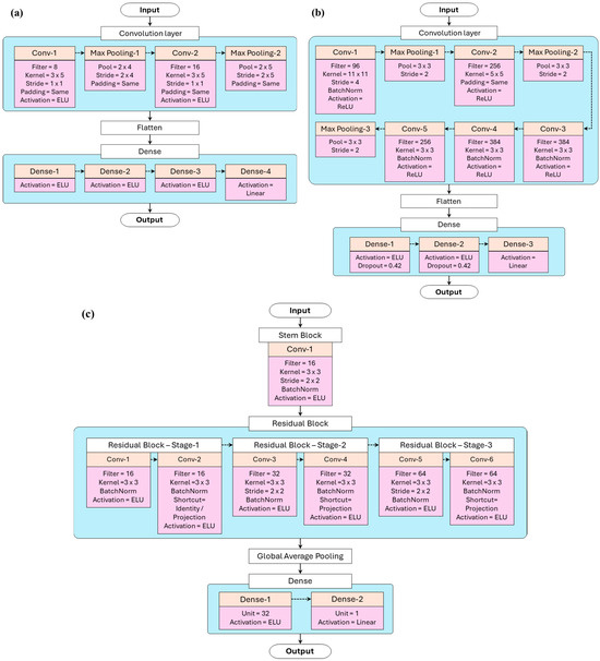
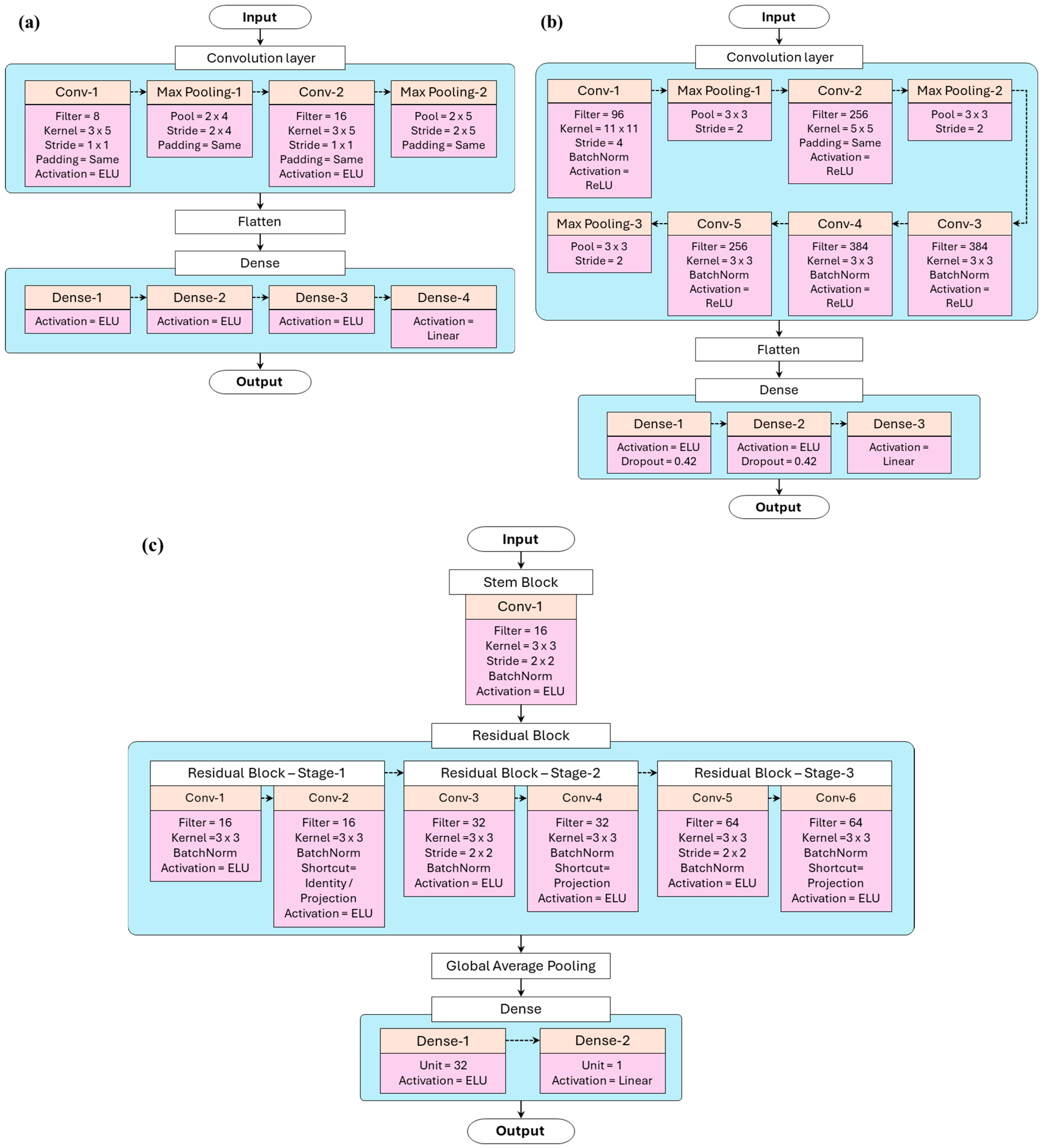
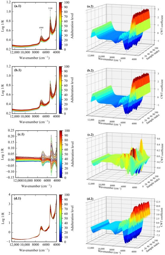
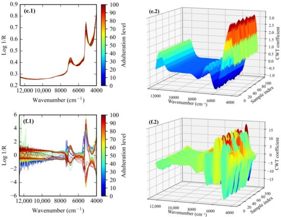
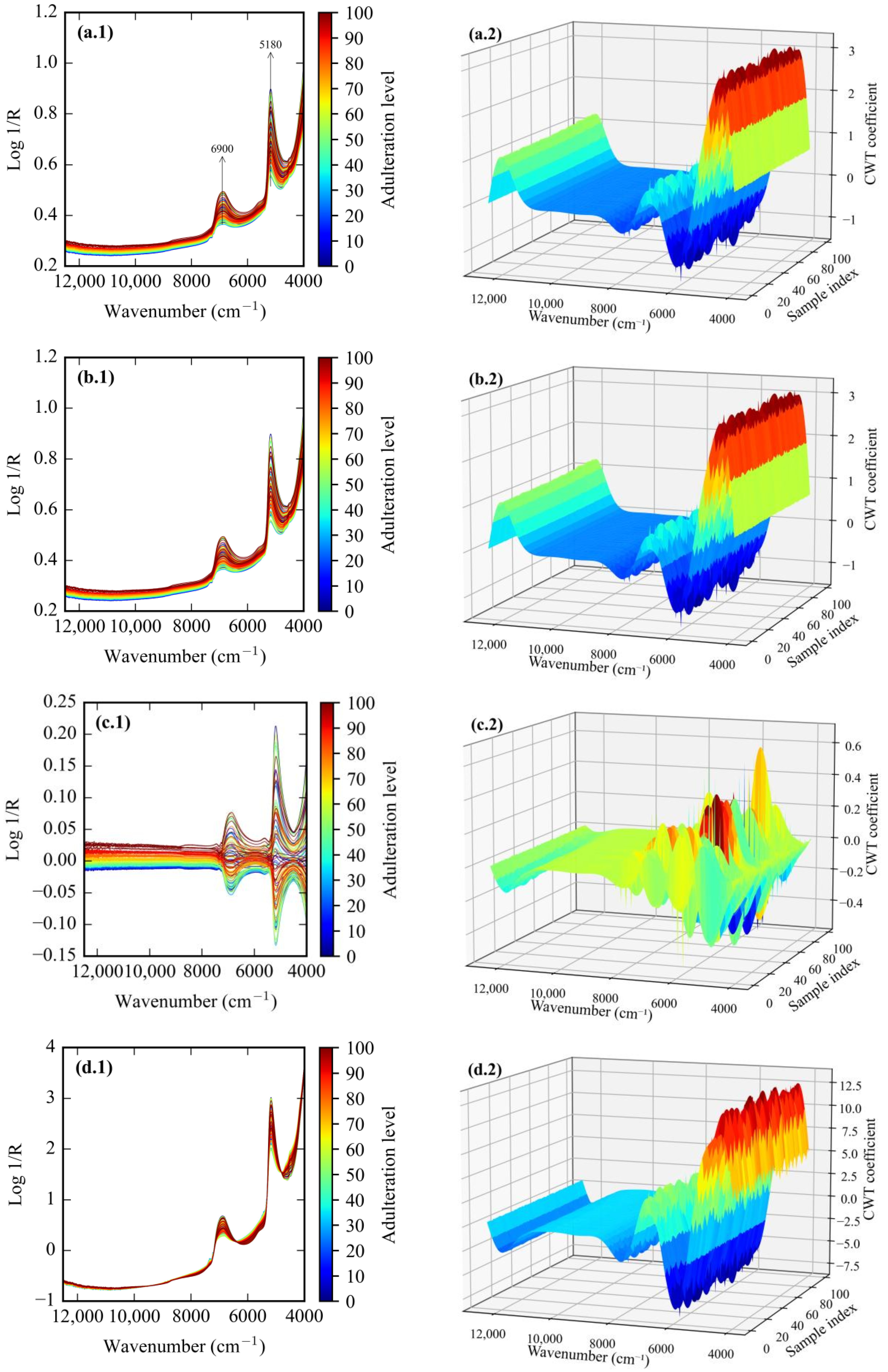
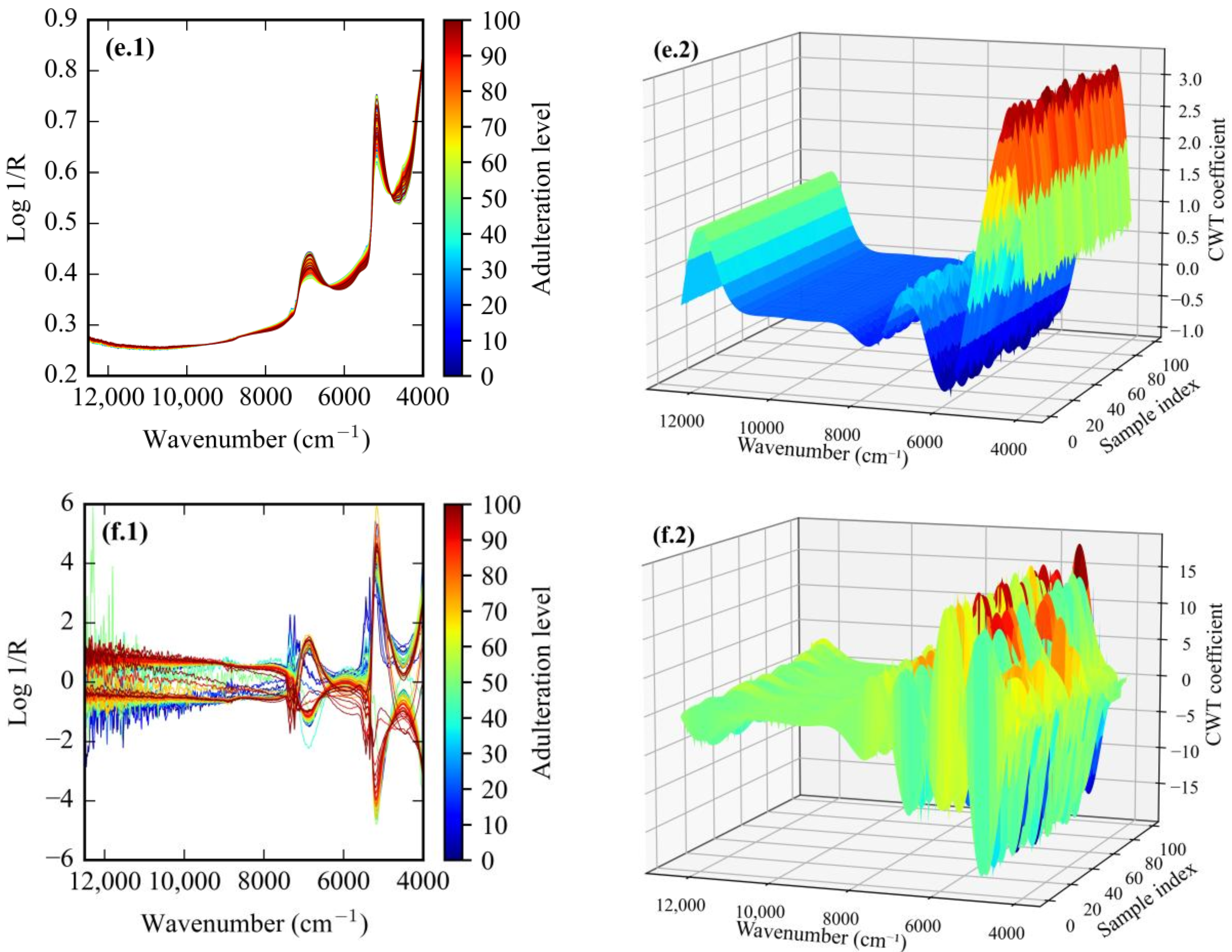
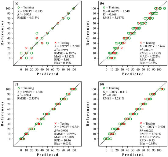
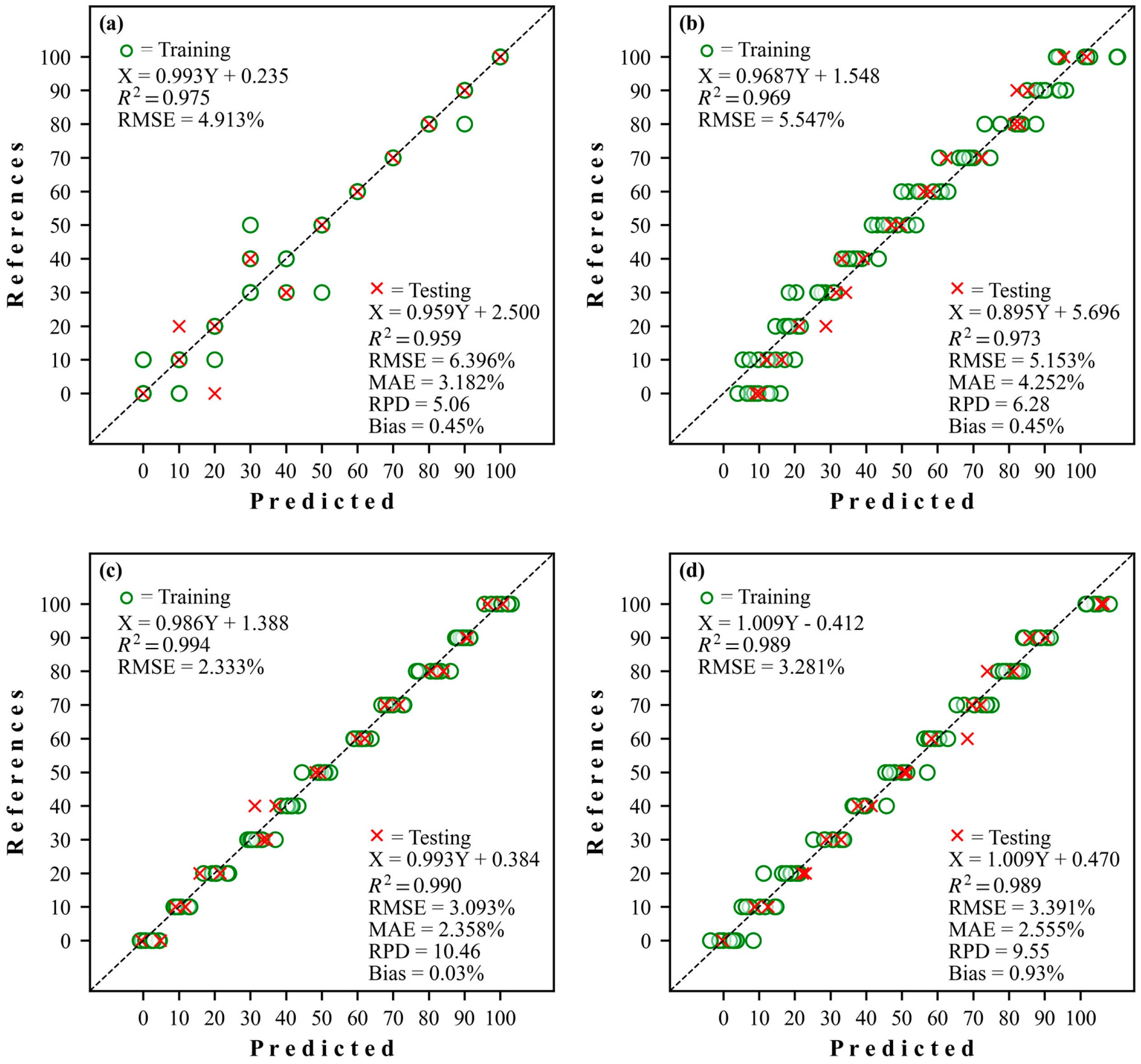
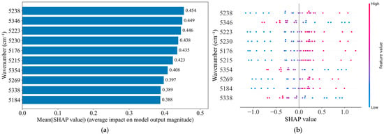
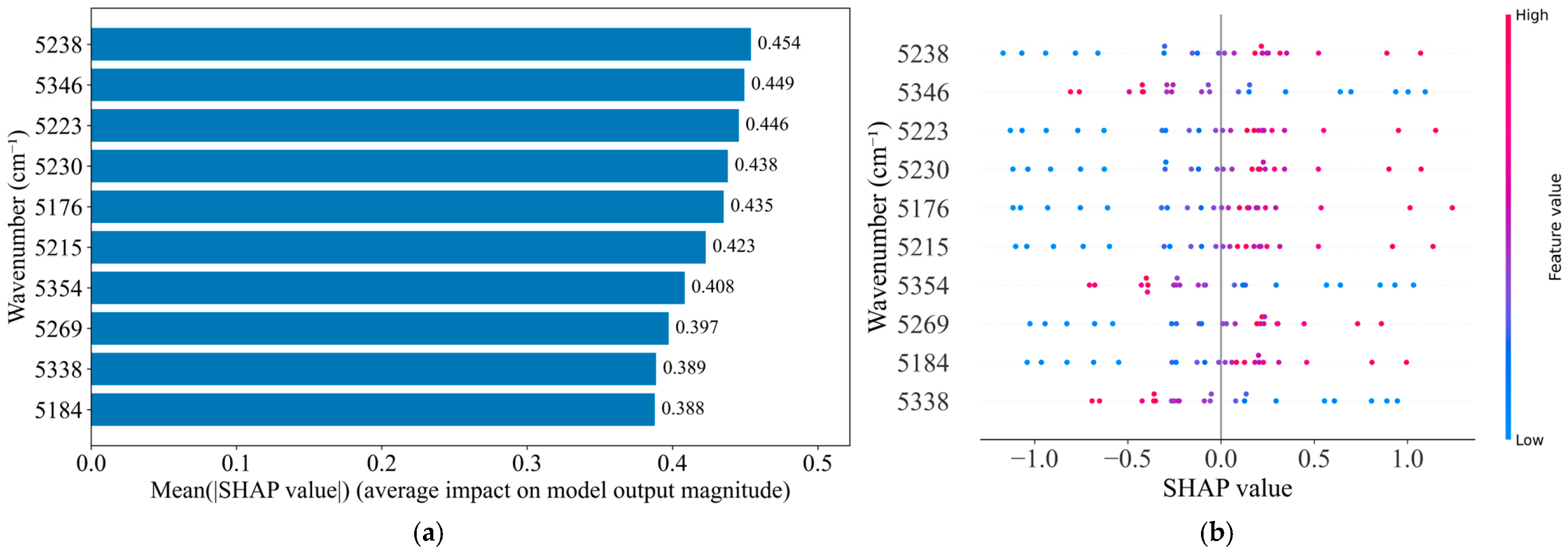
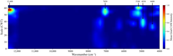
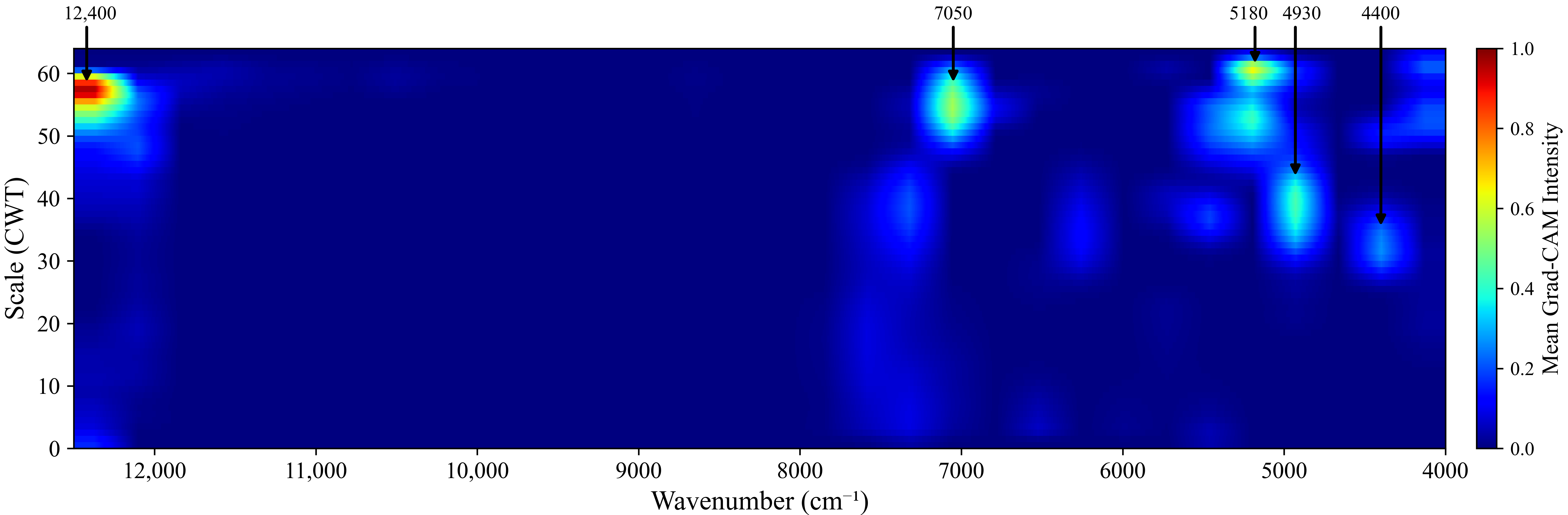

Disclaimer/Publisher’s Note: The statements, opinions and data contained in all publications are solely those of the individual author(s) and contributor(s) and not of MDPI and/or the editor(s). MDPI and/or the editor(s) disclaim responsibility for any injury to people or property resulting from any ideas, methods, instructions or products referred to in the content. |
© 2026 by the authors. Licensee MDPI, Basel, Switzerland. This article is an open access article distributed under the terms and conditions of the Creative Commons Attribution (CC BY) license.