


Abstract
Calibration of crop model parameters using optimization algorithms can substantially improve model performance, particularly under different environmental scenarios. Here, we take greenhouse drip-irrigated tomato as an example. Two temperature treatments (high temperature, TH: 35 °C ≤ Tmax ≤ 40 °C; non-high temperature, TD: Tmax ≤ 35 °C) and two water treatments (well watered, WH: 100%Epan; water deficit, WD: 60%Epan, where Epan is the pan evaporation coefficient) were combined and implemented in 2024 and 2025. Canopy cover, yield, aboveground biomass, and water consumption of tomatoes were measured, and then a global sensitivity analysis was conducted using the extended Fourier amplitude sensitivity test (EFAST). Thereafter, in order to evaluate the performance of AquaCrop-OSPy under different combinations of temperature and water conditions, the whale optimization algorithm (WOA) was coupled with the AquaCrop-OSPy model, and an automatic parameter optimization framework was developed using the aforementioned measured indicators as objective functions. The results showed that CCx, Senescence_CD, CGC_CD, WP, HI0, and Kcb were highly sensitive parameters of the AquaCrop-OSPy model across different temperature and water treatments. Compared with the traditional trial and error (TAE) method, WOA demonstrated superior global optimization capability and significantly improved model performance. Validation indicated that the root mean square error (RMSE) was ≤4.52% for canopy cover, ≤0.67 t/hm2 for yield, and ≤0.98 t/hm2 for aboveground biomass. Notably, even after WOA optimization, water consumption simulation under combined high temperature and water deficit conditions still showed some deviation, which was attributed to limitations in soil water simulation and the oversimplification of model mechanisms under combined stress. Nevertheless, the model remained reliable for estimating canopy cover, yield, and biomass, while ET simulation under combined stress should be interpreted with caution. Therefore, future improvements of AquaCrop-OSPy should focus on addressing the effects of soil water and refining the inhibitory feedback of physiological stress to better adapt the model to the combined conditions of high temperature and water deficit.
1. Introduction
As a key facility in modern protected agriculture worldwide, greenhouses can artificially regulate the microclimate to provide a favorable growing environment for crops, playing a particularly important role in enabling year-round production of fruits and vegetables and improving economic returns [1]. Owing to their advantages of low construction cost and low energy consumption, semi-open plastic greenhouses based on natural ventilation have been widely adopted across many countries [2,3,4]. To date, such greenhouses cover an area of 1.3 million hectares and constitute the predominant type of facility for protected vegetable cultivation. At present, the intensifying conflict between continued global warming and the scarcity of agricultural water resources requires the development of protected agriculture to simultaneously meet multiple objectives, such as reducing water and energy use, stabilizing and increasing yield, enhancing product quality, and improving economic benefits, thereby posing more severe practical challenges to the production and development of these simple plastic greenhouses [5,6].
In greenhouse environments, temperature and water are two key factors determining crop yield and quality. In actual production, particularly in naturally ventilated greenhouses, high temperature conditions readily occur inside the greenhouse during the spring–summer and summer–autumn periods. If water stress occurs concurrently during these periods, it can cause irreversible damage to the normal physiological metabolism of crops [7,8,9]. Conventional greenhouse environmental management often relies on growers’ experience, making it difficult to quantify the combined effects of coupled water and heat conditions on crop growth [10]. For example, an inappropriately hot and humid environment not only increases production costs but also heightens the risk of pests and diseases, whereas severe water deficit limits nutrient uptake and photosynthesis [11]. Therefore, elucidating how crops respond under different combinations of temperature and water is key to maximizing greenhouse crop yield and economic benefits.
To achieve this, advanced monitoring and predictive tools are essential. While recent progress in computer vision has enabled automated crop monitoring, yield estimation, and decision-making in precision horticulture [12], mechanistic crop growth models remain uniquely capable of quantitatively describing the underlying physiological responses to complex environmental changes. At present, mainstream crop models include DSSAT [13], WOFOST [14], APSIM [15], and AquaCrop [16], all of which have demonstrated considerable applicability in simulating different sowing dates, water and fertilizer management practices, and climate scenarios. Among them, the AquaCrop model developed by the Food and Agriculture Organization (FAO) of the United Nations is driven primarily by water. It not only inherits the capacity of physically based models to simulate physiological characteristics but also substantially simplifies parameter inputs, thereby showing a marked advantage in balancing simulation accuracy with model robustness. Numerous studies have shown that the AquaCrop model can accurately simulate canopy development, biomass accumulation, and yield formation for various crops under a range of scenarios [17,18,19]. However, previous studies have found that the simulation accuracy of the AquaCrop model under combined high temperature and water stress conditions is closely related to the accuracy of localized calibration of cultivar parameters.
At present, parameter calibration of the AquaCrop model mainly relies on the conventional trial and error (TAE) method, which is not only time-consuming and laborious but also highly prone to becoming trapped in local optima and yielding invalid parameters with degraded accuracy [20]. It is therefore necessary to develop a parameter tuning framework that balances accuracy and efficiency. Previous research has shown that a complete model parameter tuning procedure should begin with parameter sensitivity analysis, and current sensitivity analysis methods are mainly divided into local and global approaches. Conventional local sensitivity analysis varies only a single parameter at a time and neglects interaction effects among parameters, making it poorly suited to nonlinear models under dual stress [21]. Consequently, most researchers adopt global sensitivity analysis in practice. As a global sensitivity analysis method, the Morris method offers the advantage of low computational cost, but it can provide only qualitative ranking and cannot precisely quantify the magnitude of influence [22]. The Sobol’ index method achieves high accuracy but requires an extremely large sample size and entails substantial computational cost [23]. By comparison, the extended Fourier amplitude sensitivity test (EFAST) skillfully combines the strengths of variance decomposition theory and the Fourier transform, enabling both quantitative assessment of the independent effect of a single parameter and accurate capture of the total contribution of nonlinear interactions among multiple parameters, and it has been tested by numerous researchers [19]. After identifying the highly sensitive parameters, how to automatically locate the optimal parameter combination within an optimization space characterized by strong parameter interactions becomes the key to advancing model calibration. In recent years, coupling crop models with gradient-based optimization algorithms grounded in mathematical statistics and with modern metaheuristic algorithms based on swarm intelligence has been recognized as an effective approach to solving such nonlinear problems. For example, Ma et al. [24] developed an R-based DSSAT-PEST package for automatic parameter optimization and, through comparative validation across five crops, concluded that the tool outperforms conventional methods in the accuracy of parameter estimation while substantially improving operational efficiency. Wang et al. [25], drawing on field measurements from four rice cultivars, introduced the Particle Swarm Optimization (PSO) algorithm into parameter estimation for the DSSAT model and found that PSO could more stably obtain effective parameters and significantly improve the simulation accuracy of rice yield. Wu et al. [19] calibrated the AquaCrop model under coupled water, fertilizer, and biochar conditions and, in combination with the NSGA-II multi-objective optimization algorithm, identified an optimal management strategy that could synergistically enhance greenhouse tomato yield and water productivity while conserving water and fertilizer. Sharafkhane et al. [26] combined the AquaCrop model with the PSO algorithm to construct a dynamic irrigation scheduling optimization framework and, through field experiments and multi-method comparisons, demonstrated that this framework significantly outperformed conventional irrigation scheduling methods in maximizing maize water productivity. However, when confronted with highly coupled and multimodal parameter spaces, these algorithms often suffer from a loss of population diversity in the later stages of evolution, leading to premature convergence and entrapment in local optima, which limits the accuracy and robustness of the final calibration results [27,28]. The combined high temperature and water deficit stress considered in this study precisely falls into this category; it may restructure parameter sensitivity and exacerbate parameter interdependencies, thereby rendering the optimization surface multi-modal in nature. The whale optimization algorithm (WOA), which simulates the biological behavior of humpback whales, achieves a better balance between global exploration and local exploitation, enabling it to escape the premature convergence and local optima limitations commonly associated with GA and PSO. Consequently, it may be more capable of capturing optimal solutions under shifted core physiological parameters in more complex conditions [29]. It is precisely these research gaps, rather than the selection of a single optimization algorithm, that constitute the motivation of this study. To the best of our knowledge, WOA has not previously been coupled with AquaCrop-OSPy under combined heat and water stress greenhouse conditions, and its performance in such a configuration remains to be evaluated.
To address the aforementioned research gaps and challenges, we hypothesized that the global sensitivity of crop parameters in the AquaCrop-OSPy model varies systematically across different water and temperature regimes, and that coupling sensitivity-based parameter screening with intelligent optimization can substantially improve the model’s ability to reproduce the growth and water use of greenhouse-grown tomatoes. To test this hypothesis, the specific objectives of our study were to: (1) quantify and analyze the global sensitivity of the AquaCrop-OSPy crop parameters, and how it changes under different water and temperature combinations, using the EFAST method; (2) automatically optimize the highly sensitive parameters identified above using the WOA; and (3) evaluate the performance of the optimized AquaCrop-WOA coupling framework in simulating canopy cover, aboveground biomass, yield, and evapotranspiration of greenhouse tomatoes.
2. Materials and Methods
2.1. Experimental Site
The experiment was conducted from March to June in 2024 and 2025 at the Henan Key Laboratory of Water Saving Agriculture (34°47′ N, 113°39′ E, 80 m) (Figure 1). The study area has a temperate continental monsoon climate with an uneven inter-annual distribution of precipitation, most of which is concentrated in July and August. The long-term mean annual precipitation is 548 mm, the mean annual evaporation is 1909 mm, the mean annual frost-free period is 209 days, and the mean annual air temperature is 14 °C. The soil types and hydraulic properties of the 0–60 cm soil layer in the experimental area are presented in Table 1.
Figure 1.
Geographical location map of the experimental site.
Table 1.
Soil types and hydraulic parameters of the 0–60 cm soil layer inside the greenhouse.
2.2. Experimental Design
The greenhouse used in the experiment covered an area of 84 m2 (10.5 m × 8 m). It had a steel frame structure with an outer covering of a single layer of polyethylene film. The tomato cultivar was “Jingfan 404”, which was transplanted on 19 March 2024 and 15 March 2025, respectively, using an alternating planting pattern of wide rows (65 cm) and narrow rows (45 cm). On the day of transplanting, 20 mm of irrigation was applied to ensure seedling survival, and the soil surface was covered with black polyethylene film to maintain soil temperature during the seedling stage. Before transplanting, a water-soluble compound fertilizer was applied to each plot at 0.583 t/hm2; after the tomatoes entered the fruit enlargement stage, an additional 0.625 t/hm2 of water-soluble fertilizer was applied as top dressing. High temperature and ambient temperature experiments were conducted in two structurally identical greenhouses (the same model, dimensions, covering material, and ventilation configuration), with temperature as the main plot factor and water as the subplot factor, yielding four combinations in total, each replicated three times. The TH was designed such that the daily maximum air temperature was no lower than 35 °C and no higher than 40 °C, whereas the TD was designed with a daily maximum air temperature no higher than 35 °C. To avoid confounding the temperature effect with any greenhouse-specific effect, the temperature treatment was rotated between the two greenhouses across the two years: greenhouse 1 served as the high temperature unit in 2024, and greenhouse 2 served as the high temperature unit in 2025. The two water treatments were full irrigation (WH, 100%Epan) and deficit irrigation (WD, 60%Epan), where Epan is the pan evaporation coefficient. The experimental design can be referred to in [30,31]. No temperature or water treatments were applied during the seedling stage to ensure seedling survival and growth; temperature and water control treatments were initiated after the tomatoes entered the flowering and fruit setting stage.
Temperature variation inside the greenhouse was regulated by a BY-WSK IoT-based intelligent greenhouse control system (Henan Bangyou Hi-Tech Co., Zhengzhou, China), which consisted of a main control unit, a distributed temperature sensor module, and an air-cooled compressor refrigeration unit. The temperature sensors were installed at the crop canopy height and could acquire multi-point temperature data in real time and transmit them to the main control unit. During the experiment, when the outside temperature reached 35 °C, the temperature control system automatically initiated the cooling program, using cyclically operated fans together with a wet curtain water pump for cooling. One set of fans was switched every 10 min, and the temperature data were updated every 5 min. The temperature treatment was applied daily from 10:00 AM to 6:00 PM, lasting for 8 h, and was maintained for no less than 15 days in each growth stage.
The water treatments were based on the cumulative evaporation measured by a standard 20 cm pan, which was positioned 30 cm above the canopy. The daily evaporation was measured with a matching graduated cylinder between 07:30 and 08:00 each day. When the cumulative daily evaporation from the pan reached 10 ± 2 mm, irrigation was applied using drip tape with a rated flow rate of 1.1 L/h and an emitter spacing of 20 cm. In each experimental plot, the drip tape was connected to a manifold equipped with a water meter (accuracy of 0.001 m3), and all manifolds converged into a main pipeline fitted with a master water meter and a pressure gauge. Other routine agronomic management practices in the greenhouse (e.g., pest and disease control, topping, and weeding) were carried out in strict accordance with local agricultural production practices. Figure 2 shows the daily maximum and minimum temperatures and the reference evapotranspiration in the greenhouse under the two temperature treatments. Figure 3 shows the diurnal temperature variation under two temperature treatments.
Figure 2.
Changes in the daily maximum and minimum temperatures and the reference evapotranspiration in the greenhouse under TD and TH treatments.
Figure 3.
Hourly temperature variation under the TH and TD treatments. The orange dashed line marks the 35 °C threshold for the TD treatment.
2.3. Measurements and Methods
2.3.1. Meteorological Factors
Meteorological data were continuously monitored by an automatic weather station located at the center of the greenhouse, with sensors mounted 2 m above the ground. Air temperature (Ta) and relative humidity (RH) were measured using HOBO RS3-B and U23 Pro v2 data loggers (Onset Computer Corporation, Bourne, MA, USA). Solar radiation (Rs) was recorded with an LI-200X pyranometer (Campbell Scientific, Inc., Logan, UT, USA), net solar radiation (Rn) was measured with an NR-LITE2 net radiometer (Kipp & Zonen, Delft, The Netherlands), and wind speed was measured with a WindSonic ultrasonic anemometer (Gill Instruments Ltd., Lymington, Hampshire, UK). All meteorological data were collected every 5 s, averaged every 15 min, and stored in a CR1000 data logger (Campbell Scientific, Inc., Logan, UT, USA). The layout of the instruments in the greenhouse is shown in Figure 4.
Figure 4.
Layout of measuring instruments in the greenhouse.
2.3.2. Soil Water Content
Soil water content (SWC) was measured using a TRIME-IPH (IMKO, Ettlingen, Germany) time domain reflectometer. The access tubes were installed midway between two plants, and SWC was measured every 7–10 days at depths of 10, 20, 30, 40 and 60 cm below the soil surface. Each treatment was set up with three replicates. To reduce errors, the instrument was periodically calibrated against the oven-drying method using soil samples.
2.3.3. Leaf Area Index and Canopy Cover
After transplanting, three plants with similar growth vigor and health status were randomly selected and tagged. Leaf area was measured at 7-day intervals and calculated using the reduction coefficient method, and then the leaf area index (LAI) was calculated as follows:
where L is the leaf length and W is the leaf width (cm); Sl is the row spacing (cm); and Sr is the plant spacing (cm). The canopy cover (CC) was estimated from the LAI following the empirical exponential relationship based on the Beer–Lambert law adopted in the FAO AquaCrop framework [32], expressed as follows:
2.3.4. Aboveground Biomass and Yield
At each growth stage, three uniformly growing plants were selected; their roots were removed, and the stems, leaves, and fruits were separated, with the fresh weight of each part recorded. The stems, leaves, and fruits were then placed in an oven at 105 °C for 30 min for de-enzyming, followed by continuous drying at 85 °C for 12 h. The dried matter was then removed and weighed separately, and the total was taken as the aboveground biomass. In the center of each plot, 20 tomato plants were tagged for yield measurement, with three replicates per plot, and the tomato weight of each plot was measured using an electronic balance with a precision of 5 g.
2.3.5. Evapotranspiration
Evapotranspiration (ET) was calculated using the water balance method, expressed as follows:
where P is the precipitation (mm); Ir is the irrigation amount (mm); U is the groundwater recharge (mm); R is the surface runoff (mm); D is the deep percolation (mm); and ΔW is the change in water storage in the 0–60 cm soil layer (mm).
Owing to the shielding effect of the greenhouse plastic film, the precipitation inside the greenhouse was zero. The groundwater table in the study area remained below 5 m year round, so the groundwater recharge was zero. Under drip irrigation, the irrigation amount was small (the maximum single application was 13 mm); therefore, both surface runoff and deep percolation were zero [33,34,35,36]. Accordingly, the simplified water balance equation is as follows:
3. AquaCrop-OSPy Model and Its Parameters
3.1. AquaCrop-Ospy Model
The AquaCrop-OSPy model is the open source Python version 3.0.12 of the general AquaCrop model; its internal mechanisms are entirely consistent with those of AquaCrop, and it requires inputs of meteorological data, crop parameters, soil property parameters, and field management practices [37]. Figure 5 illustrates the computational principles of the AquaCrop model. The meteorological data were obtained from the weather station and mainly included the daily maximum and minimum temperatures, reference crop evapotranspiration (ET0), and precipitation. With regard to crop parameter settings, users can select an appropriate mode for simulating canopy development according to specific conditions, using either calendar days or growing degree days (GDD). In addition, the crop development process is divided into four stages: the initial canopy cover stage, the canopy development stage, the flowering and yield formation stage, and the root development stage. The calculation of actual evapotranspiration requires partitioning water consumption into two components: soil evaporation and plant transpiration. Specifically, AquaCrop-OSPy divides soil evaporation into two stages. In Stage I, the topsoil moisture is sufficient and evaporation proceeds continuously up to the limit set by the atmospheric evaporative demand, with Kr = 1 and evaporation reaching its maximum. In Stage II, after the topsoil moisture has been depleted, the rate at which deeper moisture is conducted upward is lower than the evaporative demand, so Kr begins to fall below 1 and decreases continuously, and evaporation declines accordingly. Crop transpiration is constrained by three factors: evaporative demand, canopy interception capacity, and water supply in the root zone. The model uses ET0 as the external driver and characterizes the potential transpiration capacity of the crop under its current canopy development state through the product of the crop coefficient Kcb and CC*; the larger the canopy and the higher the Kcb, the closer the potential transpiration is to the upper limit of the atmospheric evaporative demand. However, whether the potential transpiration can be realized ultimately depends on the water supply in the root zone: when the degree of root zone depletion exceeds the threshold that triggers stomatal closure, the stomatal water stress coefficient Ks,sto comes into play and proportionally reduces the actual transpiration, until transpiration ceases entirely when the root zone water is depleted to the permanent wilting point. See Equations (5)–(7) for details:
where Tr is the plant transpiration (mm); Es is the soil evaporation (mm); CC* is the actual canopy cover (%); KcTr,x is the maximum standard crop transpiration coefficient; ET0 is the reference evapotranspiration (mm/d); Kex is the maximum evaporation coefficient; and Kr is the evaporation reduction coefficient.
Figure 5.
Schematic diagram of the AquaCrop model.
For yield simulation, the aboveground biomass of the crop is determined by the linear integration of the daily normalized crop transpiration over the entire growth period (Equation (8)). During the dry matter accumulation phase, the model represents the effects of different stress factors on the crop by reducing actual transpirational water use through the simulation of physiological feedbacks, such as declining stomatal conductance, restricted canopy expansion, and accelerated leaf senescence. During the yield conversion phase, the final yield is jointly determined by the accumulated biomass and the harvest index (Equation (9)). It is worth noting that the harvest index in the model is not a static constant. Rather, it is based on the crop’s potential reference harvest index (HI0) and is dynamically adjusted through a composite adjustment factor (fHI):
where B is the biomass (t/hm2); WP is the normalized crop water productivity (g/m2); Y is the yield (t/hm2); fHI is the harvest index adjustment factor; and HI0 is the reference harvest index.
3.2. EFAST Method
The EFAST method combines the rigor of the Sobol’ method in handling higher-order parameter interactions with the computational efficiency of the FAST method, making it suitable for sensitivity analysis of nonlinear mechanistic models [38]. Based on the principle of variance decomposition, this method evaluates the sensitivity of each parameter by quantifying the contributions of individual parameter variations and inter-parameter coupling to the total variance of the model output. The first-order sensitivity index (Si) represents the direct contribution of the variation in parameter xi alone to the output variance, whereas the total sensitivity index (STi) comprehensively accounts for both the independent effect of parameter xi and its interaction effects with other parameters:
where is the sum of the variances arising from the main effects of all parameters other than xi and their interactions.
In this study, a global sensitivity analysis was performed on 43 crop parameters of the AquaCrop-OSPy model using the EFAST method implemented in the SALib library (the fast_sampler and fast modules). Unlike random Monte Carlo sampling, the EFAST method assigns a distinct characteristic frequency to each parameter and samples along the corresponding search curves in the frequency domain, and then decomposes the output variance through Fourier amplitude analysis to obtain Si and STi. To fully expose the sensitivity of each parameter across a sufficiently broad parameter space, the search range for the sensitivity analysis was set by extending each calibration bound in Table 2 outward by approximately 10%. The interference factor (number of harmonics) was set to M = 4, and the sample size was N = 1000 per parameter, giving a total of 43,000 model runs. The confidence intervals of Si and STi were estimated by bootstrap resampling (num_resamples = 100) under a fixed random seed, which also reflects the stability of the sensitivity indices under repeated resampling. A dual-threshold criterion was used to screen for highly sensitive parameters: a parameter was identified as having a significant effect when Si > 0.05 and STi > 0.1 [39].
Table 2.
Calibration results and optimization robustness metrics for the WOA and multi-start search algorithms.
3.3. Whale Optimization Algorithm
On the basis of extracting the core sensitive parameters using the EFAST method described above, the WOA was then applied to automatically optimize the highly sensitive parameters thus identified. The WOA is a metaheuristic swarm intelligence algorithm inspired by the bubble net foraging behavior of humpback whales, with advantages such as few parameter settings and a strong balance between global exploration and local exploitation. The algorithm abstracts the foraging process of humpback whales into three behavioral mechanisms—encircling prey, the bubble net attack, and random search—and performs the optimization through the dynamic switching governed by the convergence factor (which decreases linearly from 2 to 0 with the number of iterations) and the random probability p. The position update equation is as follows:
where t is the current iteration number; X*(t) is the position vector of the best solution obtained so far, which is updated in each iteration; X(t) is the position vector of the current whale individual; A and C are coefficient vectors; D = |C·X*(t) − X(t)|denotes the absolute distance between the current whale individual and the best solution; b is a constant defining the shape of the logarithmic spiral; and l is a random number uniformly distributed in [−1, 1].
Regarding the algorithm operating parameters and search boundaries, the population size of the WOA was set to 30 and the maximum number of iterations was set to 100 in this study. In this parameter calibration, the highly sensitive parameters screened by EFAST were taken as the decision variables of the WOA, and the RMSE between the simulated and measured values of CC, B, Y, and ET was used as the fitness function. Considering the marked differences in dimensions and magnitudes among the four target variables, a normalized weighted summation method based on the measured means was adopted to construct a multi-objective fitness function [40], with equal weights assigned by default (w = 0.25). The mathematical expression is as follows:
where RMSEY, RMSEB, RMSECC, and RMSEET represent the root mean square errors of the simulated yield, biomass, canopy cover, and evapotranspiration relative to their measured values, respectively; , , are the arithmetic means of the corresponding measured series; the weighting coefficients satisfy Σw = 1; and ε = 10−6 is an extremely small positive real number, used mainly to avoid numerical singularity when the measured mean approaches zero.
To assess the robustness of the optimization, the WOA was independently executed 30 times with different random seeds. The optimized parameters converged to consistent values across the runs, with coefficients of variation generally mostly below ~7% (Table 2), indicating that the results are robust and largely insensitive to initialization. A representative convergence curve is shown in Figure 6, where the fitness stabilized within 65 iterations, confirming that the selected number of iterations was sufficient for convergence. For comparison, a random multi-start search was also performed under identical conditions as a baseline; the two methods achieved comparable fitness, while the WOA yielded parameter values closer to the reference values in the AquaCrop manual, reflecting a better balance between calibration accuracy and physiological plausibility.
Figure 6.
Representative convergence curve of the WOA for parameter calibration.
4. Evaluation of Model Performance
In this study, the coefficient of determination (R2), root mean square error (RMSE), normalized root mean square error (NRMSE), Nash Sutcliffe efficiency coefficient (EF), index of agreement (dIA), and mean bias error (MBE) were selected to evaluate the performance of the model after parameter optimization. The RMSE ranges from 0 to infinity and represents the average error between the observed and simulated values. A smaller RMSE indicates higher simulation accuracy. The NRMSE is used to assess the normalized RMSE value, and its classification criteria are as follows: excellent (<10%), good (10–20%), acceptable (20–30%), and poor (>30%). R2 describes the goodness of fit of the data, with values closer to 1 indicating better model performance; a higher EF value indicates a better fit; and the index of agreement (dIA) ranges from 0 to 1, with values closer to 1 representing higher agreement. In addition, MBE reflects the direction of the systematic bias: a positive value indicates that the model overestimates the observations, whereas a negative value indicates underestimation, and a value closer to 0 indicates a smaller systematic bias. The specific formulas for these statistical indicators are as follows:
where n is the number of observations; Si and Oi represent the simulated and observed values, respectively; and and are the means of the simulated and observed values, respectively.
5. Results
5.1. Sensitivity Analysis Results of the AquaCrop-OSPy
The parameter analysis of the CC of greenhouse tomato under different water and temperature treatments is shown in Figure 7a. It is evident that the maximum canopy cover (CCx) and the time from sowing to the onset of natural canopy senescence (Senescence_CD) are relatively sensitive parameters affecting the canopy growth of greenhouse tomato. The STi were all greater than 0.1 and could therefore be identified as crop parameters with significant effects. In terms of the water effect, the sensitivity of CCx generally tended to decrease as the irrigation amount decreased, whereas the sensitivity of Senescence_CD increased as the irrigation amount decreased. In terms of the temperature effect, the overall sensitivities of both CCx and Senescence_CD increased with rising temperature, reaching their peak values under the THWH and THWD treatments, respectively (STi = 0.664 and STi = 0.267). In addition, it is worth noting that the sensitivity of the daily canopy growth rate (CGC_CD) changed with temperature; under the THWD treatment, its STi exceeded the significance threshold of 0.1, making it another sensitive parameter affecting canopy growth.
Figure 7.
Parameter sensitivity analysis for greenhouse tomato: (a) canopy cover, (b) biomass, (c) yield, and (d) evapotranspiration.
Figure 7b,c present the sensitivity analysis results for B and Y. It can be seen that the parameter sensitivity was dominated not only by the normalized water productivity (WP) and the reference harvest index (HI0) but was also significantly influenced by the maximum transpiration coefficient (Kcb), which characterizes the crop’s transpirational water use potential. It can also be observed that, as the temperature increased or the irrigation level decreased, the sensitivities of all three parameters declined to varying degrees, falling to their lowest levels across all treatments under the THWD treatment in particular (WP ≥ 0.312, HI0 ≥ 0.384, Kcb ≥ 0.096). Notably, in the biomass sensitivity analysis, the sensitivity of the CGC_CD increased under the TDWD treatment, becoming a highly sensitive parameter (STi = 0.101 > 0.1). This may be because, in the absence of temperature stress, the rate-limiting step for biomass accumulation lies in the speed of light energy interception, and CGC_CD is precisely the core parameter governing the rate of canopy expansion from emergence to development.
Figure 7d shows the parameter sensitivity analysis results for ET under different combinations of water and temperature. It can be seen that the Kcb and the CGC_CD were the main sensitive parameters affecting the water consumption process of greenhouse tomatoes, with their total order sensitivity indices being significantly greater than 0.1 under all treatments. In terms of the water effect, the sensitivity of Kcb tended to increase as the irrigation amount decreased. Here, under ambient temperature, it increased from 0.414 under full irrigation to 0.430 under water-saving irrigation, whereas under high temperature, this increase was more pronounced, rising from 0.473 to a peak of 0.512. Meanwhile, the sensitivity of CGC_CD decreased as the irrigation amount decreased. In terms of the temperature effect, the sensitivity of Kcb increased with rising temperature, being higher under high temperature than under ambient temperature in all cases, with its maximum occurring under the THWD treatment (STi = 0.512). In contrast, the sensitivity of CGC_CD showed a decreasing trend with rising temperature. Taking the water-saving irrigation treatment as an example, it decreased from 0.277 under ambient temperature to 0.156 under high temperature, with the lowest value occurring under the THWD treatment (STi = 0.156).
These results indicate that when using AquaCrop-OSPy to calibrate the parameters of greenhouse drip-irrigated tomato under different combinations of temperature and water, particular attention should be paid to CCx, Senescence_CD, CGC_CD, WP, HI0, and Kcb. Moreover, because the crop’s phenological progression and root development characteristics may undergo slight adaptive shifts relative to those under favorable environments, we recommend also calibrating the parameters with lower significant effects. MaturityCD, MaxRootingCD, SeedSize, and Zmax can capture the potential synergistic interactions among parameters within a more complete parameter space [41,42].
5.2. Parameter Calibration and Performance of TAE and WOA
Based on the results of the global sensitivity analysis described above, ten parameters were ultimately selected for calibration. The calibration was carried out using only the TDWH treatment in 2024, with four target variables (CC, B, Y, and ET) used for parameter tuning.
Two methods were used to calibrate these parameters, namely the conventional TAE method and the WOA. In the TAE method, the parameters were adjusted manually following the crop growth sequence. Canopy-related parameters such as CCx and CGC_CD were tuned first to reproduce the observed canopy cover, followed by biomass- and yield-related parameters such as WP and HI0, and finally the parameters affecting evapotranspiration. Both calibrations were performed by the same operator, used the same target variables and the same measured datasets, and adjusted the same set of parameters, while all other crop parameters were kept at their default values. The two methods therefore differ only in whether the parameters were tuned manually in the TAE method or optimized automatically by the WOA, which allows a fair comparison between them.
Each method yielded a single set of cultivar parameters (Table 3), which was then applied without any re-tuning to all other conditions for validation. The validation was conducted at two levels: (1) a cross-treatment validation, in which the parameters calibrated under the 2024 TDWH treatment were applied to the remaining water and temperature treatments in the same year; and (2) a cross-year validation, in which the same parameter set was applied to all treatments in 2025. The 2025 dataset was not involved in the calibration in any way and thus served as a fully independent validation set [43,44].
Table 3.
Calibrated parameters using the TAE method and the WOA algorithm.
This run of the WOA algorithm took about 5 min on a computer equipped with an AMD Ryzen 7 7700 processor, and the total time for 30 independent runs was approximately 2.5 h. The TAE method involved a total of 53 adjustment rounds and took approximately 37 h to reach the optimal parameter values.
5.2.1. Canopy Cover
Figure 8 compares the simulated and measured canopy cover of greenhouse drip-irrigated tomato under different temperature and water treatments after the AquaCrop-OSPy model was calibrated using the conventional TAE method and the WOA, respectively. Overall, both calibration methods were consistent with the actual growth trend of greenhouse tomato CC, and their simulation accuracy was within an acceptable range. However, the WOA showed better optimization capability on the whole. Specifically, after calibration with the WOA, the evaluation indicators were RMSE ≤ 4.52, NRMSE ≤ 7.88%, EF ≥ 0.95, dIA ≥ 0.98, and R2 ≥ 0.97. By comparison, the accuracy of the TAE method was slightly lower, with RMSE ≤ 6.90, NRMSE ≤ 11.70%, EF ≥ 0.93, dIA ≥ 0.97, and R2 ≥ 0.95 (Table 4). It should be noted that under the TH and WD conditions, the accuracy of the WOA decreased somewhat. Taking THWD in 2025 as an example, the TAE method showed a relatively obvious deviation in the middle and late parts of the growth curve, with an overall deviation of 8.32% from the measured values, whereas the deviation of the WOA was only 2.73%. This indicates that the WOA optimized the mid-stage canopy growth period without changing the basic shape of the simulated curve. The mean bias error (MBE) of each treatment further reflects this systematic bias. The MBE was positive in most cases, indicating a tendency to overestimate, while it was negative under some deficit treatments and under the 2025 conditions, corresponding to underestimation. In most treatments, the absolute MBE of the WOA was smaller than that of the TAE, indicating that the WOA also had a smaller systematic bias.
Figure 8.
Simulation of greenhouse tomato canopy cover (CC) using the AquaCrop-OSPy model calibrated by TAE and WOA.
Table 4.
Simulation of canopy cover (CC) under different water and temperature conditions using the AquaCrop-OSPy model calibrated by TAE and WOA.
5.2.2. Simulation of Yield, Biomass, and Evapotranspiration
Figure 9a,b compare the simulation results for the yield and biomass of drip-irrigated tomato under different combinations of temperature and water using the TAE method and the WOA. The fitting accuracy of both methods for yield and biomass was likewise at an acceptable level, and the accuracy of the WOA was clearly better than that of the TAE method. For the yield results in 2024, the RMSE of the WOA was 0.47 t/hm2, which is markedly lower than that of the TAE method (0.61 t/hm2), and the NRMSE was 8.33%, which is lower than that of the TAE method (11.02%). For the biomass results in 2024, the RMSE of the WOA was 0.86 t/hm2, which is markedly lower than that of the TAE method (1.01 t/hm2), and the NRMSE was 9.46%, which is lower than that of the TAE method (10.53%). For the simulation results in 2025, the TAE method showed relatively large deviations in predicting yield and aboveground biomass (RMSE ≤ 1.53 t/hm2, NRMSE ≤ 21.88%), whereas the WOA could better correct these outliers and bring the scatter points closer to the 1:1 line (RMSE ≤ 0.98 t/hm2, NRMSE ≤ 13.31%). In addition, it should be noted that most of the scatter points for both methods lay above the 1:1 line, indicating that the simulated values mostly overestimated the measured values.
Figure 9.
Comparison of fitting performance between the TAE method and the WOA for yield (a), biomass (b), and evapotranspiration (c).
Figure 9c presents the 1:1 scatter comparison of the ET simulation performance of the TAE method and the WOA for greenhouse tomato. The results showed that both methods were likewise at an acceptable level in terms of ET simulation accuracy. The evaluation indicators were as follows: for the TAE method, R2 ≥ 0.59, RMSE ≤ 67.06 mm, NRMSE ≤ 25.54%, and PE ≤ 34.19%; for the WOA, R2 ≥ 0.71, RMSE ≤ 47.75 mm, NRMSE ≤ 18.18%, and PE ≤ 27.28%. It is evident that the WOA effectively eliminated the subjectivity of manual parameter tuning. However, both calibration methods showed a certain degree of systematic overestimation of ET, and regrettably, the extent to which the WOA improved ET was relatively limited, with the error of its optimized simulated values relative to the measured values being 17.42% (compared with 24.71% for the TAE method). Notably, the model underestimated ET under the TD treatment but overestimated it under the TH treatment (Table 5).
Table 5.
Relative deviations of simulated yield, aboveground biomass, and evapotranspiration using the TAE method and the WOA under different treatments.
5.2.3. Statistical Comparison Between WOA and TAE
To evaluate whether the WOA significantly outperformed the conventional TAE method, a paired statistical comparison was performed across all validation cases. For each of the four target variables (CC, B, Y, and ET) under the four water–temperature treatments in both years, the normalized RMSE (NRMSE) of the TAE- and WOA-calibrated simulations was computed, yielding 32 paired cases. The NRMSE was used so that variables of different magnitudes could be compared on a consistent basis. Because the TAE method is a manual trial-and-error procedure that is performed only once and does not produce a distribution of results, the comparison was based on these paired NRMSE values rather than on repeated runs of the TAE method.
The WOA achieved a lower NRMSE than the TAE method in 27 of the 32 cases, and the mean NRMSE decreased from 14.17% for the TAE method to 9.91% for the WOA. A two-sided Wilcoxon signed-rank test and a two-sided paired t-test both indicated that this difference was statistically significant (Wilcoxon signed-rank test: p < 0.001; paired t-test: p < 0.001). On average, the WOA reduced the NRMSE by 4.26 percentage points, with a 95% confidence interval of [2.24, 6.28] that does not include zero. These results confirm that the WOA provided a significant and consistent improvement in calibration accuracy over the conventional TAE method across the different temperature and water regimes.
6. Discussion
6.1. Sensitivity Analysis of the AquaCrop-OSPy Parameters Under Different Temperature and Moisture Conditions
The global sensitivity analysis in this study showed that when greenhouse tomato is subjected to the combined environmental stresses of high temperature and water deficit, the sensitivity of the parameters is not fixed but evolves markedly as the combined water and heat stress intensifies. First, at the level of canopy development, the sensitivity analysis indicated that CCx and Senescence_CD played globally dominant roles, which is consistent with the findings of Wu et al. [19]. This is because they determine, respectively, the theoretical expansion limit of plant photosynthesis and the effective photosynthetic period [48]. However, this dominant role changed under the WD treatment: the sensitivity of CCx decreased, whereas that of Senescence_CD increased. From the perspective of the model’s underlying stress response mechanism, as soil water is gradually depleted, the first threshold to be triggered is the water stress threshold for leaf expansion (p-exp) rather than the threshold for stomatal closure (p-sto) [16,49]. At this point, leaf growth is directly restricted, so that the simulated canopy cover cannot reach the CCx determined by the parameter, thereby reducing the model’s dependence on CCx. At the same time, owing to the water deficit, the early senescence stress coefficient Ks,sen within the model begins to take effect; under this condition, the model assumes that the crop reduces its transpirational water use by accelerating the senescence and shedding of old leaves, which significantly shortens the effective photosynthetic duration of the canopy. The simulation of dry matter accumulation thus becomes more dependent on the timing of senescence onset, and consequently the contribution of the parameter governing the Senescence_CD to the model output variance begins to increase [50]. Notably, under TH conditions, CGC_CD became a parameter with a significant effect. A possible reason for this phenomenon is that the combined water and temperature stress altered the limiting factor for canopy development in the model. On the one hand, high temperature accelerated the accumulation of GDD, leading to a substantial shortening of the tomato growth cycle. On the other hand, the water deficit inhibited canopy expansion in the later period and induced early senescence. In this situation, the actual canopy area can hardly reach its default CCx, so the plant’s capacity to intercept light becomes more dependent on the growth rate during the early growth period. Because CGC_CD determines how quickly the initial photosynthetic area is established after emergence, the model adopts a higher CGC_CD under stress so that the plant can achieve a certain canopy cover earlier, thereby compensating for the loss of dry matter accumulation caused by the shortened growth period [51].
The formation of biomass and yield was more dependent on WP, HI0, and Kcb, which is consistent with the conclusions of Dou et al. [52], Jin et al. [53], and Wu et al. [19] on crops such as wheat, maize, and tomato. These three parameters essentially represent the genetic conversion potential of the crop cultivar under ideal conditions. When water or temperature stress is present, and especially under the combined THWD stress, the sensitivities of these parameters all declined. From the perspective of the model’s operating mechanism, the reason is as follows: when the model reads the input meteorological data, if the temperature exceeds the initially set parameter Tmax_up, the model calculates the heat stress pollination coefficient Kspol,h on each day during the pollination period and, in combination with the daily flowering proportion F (the fraction of total flowers that open on a given day during the flowering period) and the adjustment factor α for excess flowers of the crop, subsequently reduces HI0adj in a cumulative manner. At the same time, the water deficit affects HI0 and transpiration through Ks,pol and Ks,sto, respectively. In the global sensitivity variance decomposition, the degree of variation in these dynamic Ks parameters dominated the variance of the model output, and this multiplicative effect in mathematical terms weakened the dependence of the output on WP, HI0, and Kcb. By comparison, under the TDWD treatment, the sensitivity of CGC_CD began to rise. This is because, in the absence of temperature stress, the upper integration limit of the biomass equation is governed entirely by the TAW in the root zone and the timing at which stomatal closure (p-sto) is triggered, while CGC_CD directly determines the slope of the function during the early growth period. Before the available water is completely consumed and the transpiration integral is suppressed, a larger CGC_CD means that canopy closure can be completed more quickly while water is still sufficient in the early period, thereby maximizing the accumulation of effective photosynthesis and transpiration in the mathematical integration. Therefore, under the constraint of a single water stress, the model showed extremely high sensitivity to this parameter [49].
The parameter sensitivity analysis showed that, as the environmental conditions changed, the contributions of Kcb and CGC_CD to the variance of ET exhibited opposite evolutionary trends: the sensitivity of Kcb increased, whereas that of CGC_CD decreased. From the perspective of the underlying computational logic, for the AquaCrop-OSPy model, ET is mainly composed of two components, Es and Tr, superimposed together (Equation (4)), and the core equations for transpiration in the model can be found in Equations (5) and (6). When the proportion of Es decreases because of canopy shading of the soil surface, the variance of ET is mainly determined by Tr. Under the TDWH treatment, the water stress coefficient Ks = 1 and the key to the model’s calculation of cumulative water consumption lies in the dynamic integration of the actual canopy cover along the time axis. In this case, CGC_CD determines the slope of the early part of the cover growth curve and governs the expansion rate of the actual canopy cover multiplier term in the equation, thus showing a high contribution to the variance. However, in the combined THWD stress environment, the change in the meteorological input variables altered the limiting factor in the equation. On the one hand, high temperature kept ET0 at a relatively high level. On the other hand, severe water deficit first triggered the water stress coefficient for leaf expansion (Ks,exp), and the actual canopy cover was confined to a relatively low threshold. After Ks,exp intervened as a multiplier, the magnitude of the effect of variation in CGC_CD on CC was compressed proportionally, so that its contribution was diluted in the variance decomposition, leading to a decline in its contribution to the total variance. At the same time, because the external ET0 multiplier term was relatively high, the contributions of all multipliers CC* and Kcb in the calculation of the Tr equation to the output variance would be amplified proportionally (Equation (5)). However, because CC* was compressed to a relatively low and relatively fixed value by the water stress, its range of variation narrowed, and Tr was then constrained by the parameter Kcb that represents the calibrated theoretical transpiration potential. In this constrained system of multiplicative equations, Kcb, as the key multiplier that directly amplifies or reduces the transpiration base, gained increased computational weight, which caused its STi to reach its highest level under the THWD treatment [54].
6.2. Automatic Optimization and Simulation Using the WOA
This study used the TAE method and the WOA in combination with the AquaCrop-OSPy model to simulate and evaluate the canopy cover, yield, aboveground biomass, and evapotranspiration of greenhouse tomato under different water and temperature conditions. Overall, the accuracy of both methods was satisfactory, but the accuracy of the WOA was better than that of the TAE method on the whole. Except for the optimization of the simulated ET, which was not significant, the WOA showed a high optimization capability for all other indicators. This is because the TAE method is essentially a univariate local adjustment process based on prior experience. In a model such as AquaCrop-OSPy that involves complex physiological processes, there are often relatively strong coupling effects and equifinality among the input parameters, making it difficult to simultaneously find the global optimal solution among the different variation states of multiple parameters, and it is prone to becoming trapped in a local optimum during the optimization process. This phenomenon was more pronounced under the high temperature treatments. The advantage of the WOA over the TAE method was amplified as the combined water and heat stress intensified. Under the TDWH treatment, the difference in accuracy between the two was small, whereas under the combined THWD stress, the WOA reduced the RMSE of CC from 6.90 to 4.52 (a reduction of 34.5%). This is because high temperature reorganized the parameter sensitivities and strengthened the parameter coupling, making the optimization surface more multimodal. The parameter combinations obtained by the step by step tuning of the TAE method lost their adaptability, whereas the WOA was able to escape this through global exploration. Its advantage was therefore most prominent precisely under high temperature scenarios.
For canopy cover, we found that under the TH and WD treatments, the overall simulation accuracy of the model decreased to a certain extent regardless of whether the TAE method or the WOA was used, and this was most pronounced under the THWD treatment. This is mainly constrained by the structural simplification of the model itself. When greenhouse tomato actually experiences high temperature, this is often accompanied by complex photosynthetic enzyme inactivation and irreversible tissue damage, whereas the temperature stress response function within AquaCrop is relatively conservative and can hardly fully characterize such nonlinear physiological decline [55]. Therefore, even if the intelligent algorithm finds the mathematically optimal solution under the current model structure, it cannot compensate for the error caused by the limitations of the model mechanism itself. In addition, both the TAE method and the WOA generally underestimated the measured values in the early developmental period, which is consistent with the findings of Cheng et al. [56] and Lyu et al. [57], and the WOA did not noticeably correct this deviation. This early underestimation may not stem from an insufficient parameter optimization capability of the algorithm, but rather from the difference between the model’s water balance algorithm for homogeneous layered soil and the actual environment of the greenhouse during the early period. As a water-driven model, AquaCrop judges whether canopy expansion is subject to water stress on the basis of the ratio of the root zone water depletion (Dr) to the TAW, that is, the depletion fraction; when the depletion fraction Dr/TAW is greater than the Pexp (the soil water depletion fraction at which canopy expansion begins to be inhibited) threshold, water stress occurs [21]. However, in the early simulation period, the initial root depth of tomato is shallow and water uptake is mainly concentrated in the surface soil, so that even the depletion of the surface soil is sufficient to push the root zone depletion fraction close to or even beyond the stress-triggering threshold. As a result, the model prematurely judges that the crop has already experienced water stress, whereas in the early period of the actual greenhouse, no water deficit treatment is usually applied in order to ensure seedling survival. This deviation from the actual environment leads to a systematic underestimation of the measured canopy cover by the simulated values [32]. This further indicates that when AquaCrop-OSPy is applied to the refined management of protected greenhouses, its accuracy depends not only on a highly robust intelligent algorithm for optimizing physiological parameters, but also on an effective correction of the model’s early soil moisture boundary conditions and stress-triggering logic.
In addition, the validation results showed that most of the scatter points for both methods lay above the 1:1 line for yield and biomass, indicating that the model tends to systematically overestimate the actual yield and biomass, which is consistent with the conclusions of Razzaghi et al. [58] and Zhang et al. [8]. The reason for this phenomenon is that the model’s assumption of an upper limit on the theoretical potential and its oversimplified representation of crop growth responses under stress conditions together lead to the deviation whereby the simulated values are generally higher than the measured values. On the one hand, the essence of the AquaCrop output is the attainable production potential constrained by water and heat conditions; in the idealized computational environment of the model, the crop does not suffer the yield losses caused by pests, diseases, and weed competition that are unavoidable in reality. On the other hand, the model has limitations in its mechanism under high temperature stress. For the plant, the yield reduction caused by high temperature mainly originates from reduced photosynthetic rate and reduced biomass accumulation [59]. However, the current model does not have a carbon module that directly simulates photosynthesis, and its response to environmental stress relies mainly on an empirical penalty coefficient Ks ranging from 0 to 1. This relatively conservative and simplified mathematical attenuation mechanism can hardly characterize the systematic physiological responses of the crop under stress environments.
It must be noted that the accuracy with which the WOA optimized ET was not significant compared with the TAE method. The overall simulated values after optimization showed an error relative to the measured values that was only 7.29% lower than that of the TAE method. We also found an underestimation of ET under the TD treatment, which is consistent with the findings of Khorsand et al. [60] and Wu et al. [61]. The reason lies in the inherent deficiency of the model in simulating SWC. During the early and middle stages of canopy development, Es predominates; in actual drip irrigation, water is concentrated near the root zone and forms a localized elliptical wetted region, and the surface soil near the emitter constantly maintains a relatively high water content and can sustain normal evaporation. However, although AquaCrop introduces the surface wetted fraction parameter (fw) to correct soil evaporation under drip irrigation, the model is based on a one-dimensional vertical water balance algorithm at its core and is more oriented toward the vertical movement of water, making it difficult to characterize the lateral diffusion of water within the drip irrigation wetted body. As a result, between two irrigation events, the model assumes that the surface soil can sustain evaporation only by relying on the vertical water remaining from the previous irrigation, and it cannot perceive the process by which the drip irrigation wetted body actually continues to replenish water laterally to the surface layer. This causes the model to wrongly assume that the surface water is consumed faster than it actually is, to judge prematurely that the evaporable water in the surface layer has been exhausted, and thus to switch prematurely from Stage I to Stage II, with the evaporation reduction coefficient (Kr) intervening early to reduce evaporation, ultimately resulting in a systematic underestimation of soil evaporation [60]. Notably, we also found that ET under the high temperature scenario was overestimated in the middle and late growth stages. From the perspective of the model, when the canopy cover reaches the set CCx, Es accounts for a lower proportion owing to canopy closure and shifts to being dominated by Tr; because high temperature increases the vapor pressure deficit (VPD), the ET0 increases accordingly, thereby leading to an increase in Tr [62]. On the other hand, the parameter pupper that controls stomatal closure in the model is essentially a threshold defined on the basis of the depletion fraction of available water in the root zone soil, which is a typical water supply-driven mechanism. In the later period of the high temperature treatment, because the irrigation amount was relatively sufficient, the depletion fraction of root zone soil water did not reach the pupper threshold, so the model judged that the water supply was sufficient and the stomata remained open, so that Tr continued to increase even under the high temperature environment. However, from the perspective of the plant, in an actual high temperature greenhouse environment, when tomato encounters high temperature it will actively or passively close its stomata in order to reduce transpirational water loss from within the plant, leading to a decline in the actual plant transpiration.
The above analysis indicates that the ET simulation bias of the AquaCrop-OSPy model under combined stress mainly arises from limitations at the structural level, which also points to directions for future improvement. To address the underestimation of ET under water deficit, one option is to improve the model structure itself by incorporating a two-dimensional or lateral soil water redistribution module or refining the soil-evaporation algorithm under drip irrigation and mulch, so as to more realistically represent the water movement within the drip irrigation wetting bulb. Alternatively, a data-driven approach could be adopted, in which the residuals between the measured and simulated soil water content, together with meteorological variables, are used to train a machine learning or deep learning model to correct the simulated soil water content through residual learning, thereby mitigating the systematic bias without altering the main model structure [63,64]. To address the overestimation of ET under high temperature, a temperature-driven stomatal-closure mechanism could be introduced in addition to the existing water-supply-driven threshold (pupper), enabling the model to respond to heat stress and capture heat-induced stomatal closure even when soil water is sufficient. These improvements are expected to further enhance the applicability of the AquaCrop-OSPy model under combined high temperature and water deficit stress.
6.3. Practical Implications for Greenhouse Tomato Production
The proposed WOA–AquaCrop-OSPy framework offers several practical benefits for greenhouse tomato production. First, the improved prediction of yield and biomass allows growers to estimate the timing and quantity of harvest more reliably under different temperature and water regimes, which can support labor scheduling, packaging, and marketing decisions. Second, because the calibrated model reproduces canopy development and biomass accumulation well, it can help growers compare crop responses to different irrigation levels and identify water-saving strategies that maintain yield; however, given the residual bias in the absolute ET simulation under combined stress, the model is currently better-suited to comparing relative irrigation scenarios than to prescribing exact absolute irrigation amounts, and ET-based scheduling should be applied with greater caution. Third, more reliable yield prediction can reduce the risk of over or underestimating production, thereby improving the planning of inputs and marketing; a quantitative economic analysis was beyond the scope of this study but represents a valuable direction for future work. Finally, the framework itself is general and can be transferred to other cultivars and greenhouse systems: as HI0 and several other parameters are cultivar-specific, application to a new cultivar or greenhouse type would require re-calibrating these parameters using local measurements, but the same EFAST screening and WOA calibration procedure can be applied directly.
7. Conclusions
This study used the EFAST method to perform a parameter sensitivity analysis of the AquaCrop-OSPy model under the scenario of greenhouse drip-irrigated tomato and combined it with the WOA to construct a coupled framework for automatic parameter optimization, with the aim of optimizing the performance of the AquaCrop-OSPy model for canopy cover, yield, aboveground biomass, and water consumption under different temperature and water treatments. The sensitivity analysis results showed that, in the parameter calibration of drip-irrigated tomato, particular attention should be paid to CCx, Senescence_CD, CGC_CD, WP, HI0, and Kcb. The cultivar parameters calibrated by the TAE method and the WOA performed well in simulating canopy cover, yield, and biomass, and the calibration accuracy of the WOA was better than that of the TAE method. However, the optimization of water consumption by both algorithms was not significant compared with the original, and obvious deviations occurred especially under high temperature and water deficit scenarios. It should be noted that this deviation was confined to water consumption; the model remained reliable in simulating canopy cover, yield, and biomass, and is therefore still valuable for crop growth and yield prediction under these conditions. Therefore, in greenhouse tomato simulations involving high temperature scenarios, relying solely on mathematical parameter calibration is insufficient, and future model optimization should focus on correcting the physiological mechanisms and the soil-moisture simulation logic of the model under extreme stress conditions.
Author Contributions
Conceptualization, W.Z. and X.G.; methodology, W.Z., X.G. and R.Q.; software, W.Z. and X.G.; validation, W.Z., X.G. and T.R.; formal analysis, W.Z., X.G., T.R. and R.Q.; investigation, W.Z., X.G., T.R. and X.W.; resources, J.G., Y.L. and H.L.; data curation, W.Z., X.G., T.R., S.C. and Y.L.; writing—original draft preparation, W.Z. and T.R.; writing—review and editing, W.Z., X.G., J.L. and R.Q.; supervision, X.G.; project administration, X.G.; funding acquisition, X.G. and R.Q. All authors have read and agreed to the published version of the manuscript.
Funding
This research was funded by the Natural Science Foundation of Henan Province, grant number 262300421363; the Key Scientific Research Project of Higher Education Institutions in Henan Province, grant number 26A570003; and National Natural Science Foundation of China, grant number 52322904.
Data Availability Statement
The original contributions presented in this study are included in the article. Further inquiries can be directed to the corresponding author.
Acknowledgments
The authors thank the Institute of Farmland Irrigation, Chinese Academy of Agricultural Sciences, Xinxiang, for the agronomic support.
Conflicts of Interest
The authors declare no conflicts of interest.
References
- Zhang, J.; Xiang, L.; Zhu, C.; Li, W.; Jing, D.; Zhang, L.; Liu, Y.; Li, T.; Li, J. Evaluating the irrigation schedules of greenhouse tomato by simulating soil water balance under drip irrigation. Agric. Water Manag. 2022, 283, 108323. [Google Scholar]
- Gumisiriza, M.S.; Ndakidemi, P.; Nalunga, A.; Mbega, E.R. Building sustainable societies through vertical soilless farming: A cost-effectiveness analysis on a small-scale non-greenhouse hydroponic system. Sustain. Cities Soc. 2022, 83, 103923. [Google Scholar] [CrossRef] [Scilit]
- Niu, B.; Feng, Q.; Qiu, B.; Su, S.; Zhang, X.; Cui, R.; Zhang, X.; Sun, F.; Yan, W.; Zhao, S.; et al. Global-PCG-10: A 10 m global map of plastic-covered greenhouses derived from Sentinel-2 in 2020. Earth Syst. Sci. Data Discuss. 2025, 17, 5065–5088. [Google Scholar] [CrossRef] [Scilit]
- Sun, W.; Wei, X.; Zhou, B.; Lu, C.; Guo, W. Greenhouse heating by energy transfer between greenhouses: System design and implementation. Appl. Energy 2022, 325, 119815. [Google Scholar] [CrossRef] [Scilit]
- Liu, H.; Yin, C.; Gao, Z.; Hou, L. Evaluation of cucumber yield, economic benefit and water productivity under different soil matric potentials in solar greenhouses in North China. Agric. Water Manag. 2021, 243, 106442. [Google Scholar] [CrossRef] [Scilit]
- Wang, Q.; Jia, Y.; Pang, Z.; Zhou, J.; Scriber, K.E., II; Liang, B.; Chen, Z. Intelligent fertigation improves tomato yield and quality and water and nutrient use efficiency in solar greenhouse production. Agric. Water Manag. 2024, 298, 108873. [Google Scholar] [CrossRef] [Scilit]
- Ge, J.; Liu, H.; Gong, X.; Yu, Z.; Li, L.; Li, Y. Root distribution of Tomato cultivated in greenhouse under different ventilation and water conditions. Plants 2023, 12, 1625. [Google Scholar] [CrossRef] [Scilit] [PubMed]
- Zhang, J.; Li, K.; Gao, Y.; Feng, D.; Zheng, C.; Cao, C.; Sun, J.; Dang, H.; Hamani, A.K.M. Evaluation of saline water irrigation on cotton growth and yield using the AquaCrop crop simulation model. Agric. Water Manag. 2022, 261, 107355. [Google Scholar] [CrossRef] [Scilit]
- Gong, X.; Zeng, W.; Ren, T.; Li, Y.; Ge, J.; Li, Y.; Wu, X.; Zhang, T.; Li, H.; Qiu, R. Multi-Temporal Spectral Characteristics of Evapotranspiration in Greenhouse-Grown Tomato Under Deficit Irrigation Management. Agronomy 2026, 16, 1040. [Google Scholar] [CrossRef] [Scilit]
- Sun, L.; Li, B.; Yao, M.; Niu, D.; Gao, M.; Mao, L.; Xu, Z.; Wang, T.; Wang, J. Optimising water and nitrogen management for greenhouse tomatoes in Northeast China using EWM−TOPSIS−AISM model. Agric. Water Manag. 2023, 290, 108579. [Google Scholar] [CrossRef] [Scilit]
- Diouf, I.A.; Derivot, L.; Bitton, F.; Pascual, L.; Causse, M. Water deficit and salinity stress reveal many specific QTL for plant growth and fruit quality traits in tomato. Front. Plant. Sci. 2018, 9, 279. [Google Scholar] [CrossRef] [Scilit] [PubMed]
- Rana, S.; Hensel, O.; Nasirahmadi, A. From vineyard to vision: Multi-domain analysis and mitigation of grape cluster detection failures in complex viticultural environments. Results Eng. 2026, 29, 108833. [Google Scholar] [CrossRef] [Scilit]
- Jones, J.W.; Hoogenboom, G.; Porter, C.H.; Boote, K.J.; Batchelor, W.D.; Hunt, L.A.; Wilkens, P.W.; Singh, U.; Gijsman, A.J.; Ritchie, J.T. The DSSAT cropping system model. Eur. J. Agron. 2003, 18, 235–265. [Google Scholar] [CrossRef] [Scilit]
- de Wit, A.H.D.S. 25 years of the WOFOST cropping systems model. Agric. Syst. 2019, 168, 154–167. [Google Scholar] [CrossRef] [Scilit]
- Keating, B.A.; Carberry, P.S.; Hammer, G.L.; Probert, M.E.; Robertson, M.J.; Holzworth, D.; Huth, N.I.; Hargreaves, J.N.G.; Meinke, H.; Hochman, Z.; et al. An overview of APSIM, a model designed for farming systems simulation. Eur. J. Agron. 2003, 18, 267–288. [Google Scholar] [CrossRef] [Scilit]
- Vanuytrecht, E.; Raes, D.; Steduto, P.; Hsiao, T.C.; Fereres, E.; Heng, L.K.; Vila, M.G.; Moreno, P.M. AquaCrop: FAO’s crop water productivity and yield response model. Environ. Model. Softw. 2014, 62, 351–360. [Google Scholar] [CrossRef] [Scilit]
- Benard, D.N.; Obiero, J.P.O.; Mbuge, D.O.; Marta, A.D. Modelling of Cowpea response to varying irrigation and SAP levels under greenhouse conditions using AquaCrop. Irrig. Drain. 2025, 74, 1253–1266. [Google Scholar] [CrossRef] [Scilit]
- Khafajeh, H.; Banakar, A.; Minaei, S.; Delavar, M. Evaluation of AquaCrop model of cucumber under greenhouse cultivation. J. Agric. Sci. 2021, 158, 845–854. [Google Scholar]
- Wu, K.; Zhao, W.; Wu, Y.; Yu, H.; Zhou, C. EFAST-based global sensitivity analysis of the AquaCrop model and optimization of water, fertilizer, and biochar management in greenhouse tomato production. Eur. J. Agron. 2026, 178, 128118. [Google Scholar] [CrossRef] [Scilit]
- Boulange, J.; Nizamov, S.; Nurbekov, A.; Ziyatov, M.; Kamilov, B.; Nizamov, S.; Abduvasikov, A.; Khamdamova, G.; Watanabe, H. Calibration and validation of the AquaCrop model for simulating cotton growth under a semi-arid climate in Uzbekistan. Agric. Water Manag. 2025, 310, 109360. [Google Scholar] [CrossRef] [Scilit]
- Saltelli, A.; Aleksankina, K.; Becker, W.; Fennell, P.; Ferretti, F.; Holst, N.; Li, S.; Wu, Q. Why so many published sensitivity analyses are false: A systematic review of sensitivity analysis practices. Environ. Model. Softw. 2019, 114, 29–39. [Google Scholar] [CrossRef] [Scilit]
- Campolongo, F.; Cariboni, J.; Saltelli, A. An effective screening design for sensitivity analysis of large models. Environ. Model. Softw. 2007, 20, 1509–1518. [Google Scholar] [CrossRef] [Scilit]
- Nossent, J.; Elsen, P.; Bauwens, W. Sobol’ sensitivity analysis of a complex environmental model. Environ. Model. Softw. 2011, 26, 1515–1525. [Google Scholar] [CrossRef] [Scilit]
- Ma, H.; Malone, R.W.; Jiang, T.; Yao, N.; Chen, S.; Song, L.; Feng, H.; Yu, Q.; He, J. Estimating crop genetic parameters for DSSAT with modified PEST software. Eur. J. Agron. 2020, 115, 126017. [Google Scholar] [CrossRef] [Scilit]
- Wang, B.; Yang, H.; Feng, J.; Guo, Z.; Guo, Y. Rice genotype coefficient optimization of DSSAT based on PSO. Trans. Chin. Soc. Agric. Mach. 2023, 54, 369–375. [Google Scholar]
- Sharafkhane, M.G.; Ziaei, A.N.; Naghedifar, S.M.; Akbari, A.; Verdi, A. AquaCrop Plug-in-PSO: A novel irrigation scheduling optimization framework for maize to maximize crop water productivity using in-season weather forecast and crop yield estimation. Agric. Water Manag. 2024, 306, 109153. [Google Scholar] [CrossRef] [Scilit]
- Arsenault, R.; Poulin, A.; Côté, P.; Brissette, F. Comparison of stochastic optimization algorithms in hydrological model calibration. J. Hydrol. Eng. 2013, 19, 1374–1384. [Google Scholar] [CrossRef] [Scilit]
- Shami, T.M.; El-Saleh, A.A.; Alswaitti, M.; Al-Tashi, Q.; Summakieh, M.A.; Mirjalili, S. Particle swarm optimization: A comprehensive survey. IEEE Access 2022, 10, 10031–10061. [Google Scholar] [CrossRef] [Scilit]
- Mirjalili, S.; Lewis, A. The Whale Optimization Algorithm. Adv. Eng. Softw. 2016, 95, 51–67. [Google Scholar] [CrossRef] [Scilit]
- Hasanuzzaman, M.; Bhuyan, M.H.M.B.; Anee, T.I.; Parvin, K.; Nahar, K.; Mahmud, J.A.; Fujita, M. Regulation of ascorbate-glutathione pathway in mitigating oxidative damage in plants under abiotic stress. Antioxidants 2019, 8, 384. [Google Scholar] [CrossRef] [Scilit] [PubMed]
- Locatelli, S.; Jr, W.B.; Verdi, L.; Nicoletto, C.; Marta, A.D.; Maucieri, C. Modelling the response of tomato on deficit irrigation under greenhouse conditions. Sci. Hortic. 2024, 326, 112770. [Google Scholar] [CrossRef] [Scilit]
- Hsiao, T.C.; Heng, L.; Steduto, P.; Rojas-Lara, B.; Raes, D.; Fereres, E. AquaCrop—The FAO crop model to simulate yield response to water: III. parameterization and testing for maize. Agron. J. 2009, 101, 448–459. [Google Scholar] [CrossRef] [Scilit]
- Sun, L.; Li, B.; Yao, M.; Mao, L.; Zhao, M.; Niu, H.; Xu, Z.; Wang, T.; Wang, J. Simulation of soil water movement and root uptake under mulched drip irrigation of greenhouse tomatoes. Water 2023, 15, 1282. [Google Scholar] [CrossRef] [Scilit]
- Zheng, J.; Huang, G.; Jia, D.; Wang, J.; Mota, M.; Pereira, L.; Huang, Q.; Xu, X.; Liu, H. Responses of drip irrigated tomato (Solanum lycopersicum L.) yield, quality and water productivity to various soil matric potential thresholds in an arid region of Northwest China. Agric. Water Manag. 2013, 129, 181–193. [Google Scholar] [CrossRef] [Scilit]
- Ge, J.; Gong, X.; Liu, Y.; Chen, H.; Sun, H.; Traore, S.; Zhang, L. The potential effects of drip irrigation on soil environment root distribution and yield of greenhouse tomato. Eur. J. Hortic. Sci. 2022, 87, 11. [Google Scholar] [CrossRef] [Scilit]
- Sandhu, R.; Irmak, S. Assessment of AquaCrop model in simulating maize canopy cover, soil-water, evapotranspiration, yield, and water productivity for different planting dates and densities under irrigated and rainfed conditions. Agric. Water Manag. 2019, 224, 105753. [Google Scholar] [CrossRef] [Scilit]
- Feng, D.; Li, G.; Wang, D.; Wulazibieke, M.; Cai, M.; Kang, J.; Yuan, Z.; Xu, H. Evaluation of AquaCrop model performance under mulched drip irrigation for maize in Northeast China. Agric. Water Manag. 2022, 261, 107372. [Google Scholar] [CrossRef] [Scilit]
- Tian, Y.; Pan, C.; Guo, Z.; Du, L.; Xu, L.; Xiong, Y.; Huang, G. Global sensitivity analysis of crop and soil parameters of CERES-Maize model under different irrigation and fertilization regimes based on the EFAST method. Agric. Water Manag. 2026, 328, 110311. [Google Scholar] [CrossRef] [Scilit]
- DeJonge, K.C.; Ascough, J.C., II; Ahmadi, M.; Andales, A.A.; Arabi, M. Global sensitivity and uncertainty analysis of a dynamic agroecosystem model under different irrigation treatments. Ecol. Model. 2012, 231, 113–125. [Google Scholar] [CrossRef] [Scilit]
- Marler, R.T.; Arora, J.S. Survey of multi-objective optimization methods for engineering. Struct. Multidiscip. Optim. 2004, 26, 369–395. [Google Scholar] [CrossRef] [Scilit]
- Akbari, E.; Boloorani, A.D.; Verrelst, J.; Pignatti, S.; Samany, N.N.; Soufizadeh, S.; Hamzeh, S. How global sensitive is the AquaCrop model to input parameters? A case study of silage maize yield on a regional scale. Front. Agron. 2024, 6, 1304611. [Google Scholar] [CrossRef] [Scilit]
- Shanono, N.J.; Ahmad, L.; Nasidi, N.M.; Jibril, A.N.; Yahya, M.N. Simulation-optimization modelling of yield and yield components of tomato crop. Turk. J. Agric. Eng. Res. 2023, 4, 104–124. [Google Scholar] [CrossRef] [Scilit]
- Darko, R.O.; Shouqi, Y.; Haofang, Y.; Liu, J.; Abbey, A. Calibration and validation of AquaCrop for deficit and full irrigation of tomato. Int. J. Agric. Biol. Eng. 2016, 9, 104–110. [Google Scholar]
- Khorsand, A.; Dehghanisanij, H.; Heris, A.M.; Asgarzadeh, H.; Rezaverdinejad, V. Calibration and evaluation of the FAO AquaCrop model for canola (Brassica napus) under full and deficit irrigation in a semi-arid region. Appl. Water Sci. 2024, 14, 56. [Google Scholar] [CrossRef] [Scilit]
- Allen, R.G.; Pereira, L.S.; Raes, D.; Smith, M. FAO Irrigation and Drainage Paper No. 56; Food and Agriculture Organization of the United Nations: Rome, Italy, 1998. [Google Scholar]
- Baştuğ, R.; Büyüktaş, D.; Büyüktaş, K.; Aydinsakir, K.; Onus, A.N.; Karaca, C. Evapotranspiration and crop coefficients of some vegetable crops grown under greenhouse conditions. J. Water Clim. Change 2024, 15, 3236–3259. [Google Scholar] [CrossRef] [Scilit]
- Orgaz, F.; Fernández, M.D.; Bonachela, S.; Gallardo, M.; Fereres, E. Evapotranspiration of horticultural crops in an unheated plastic greenhouse. Agric. Water Manag. 2005, 72, 81–96. [Google Scholar] [CrossRef] [Scilit]
- Raes, D.; Steduto, P.; Hsiao, T.C.; Fereres, E. AquaCrop—The FAO crop model to simulate yield response to water: II. main algorithms and software description. Agron. J. 2009, 101, 438–447. [Google Scholar] [CrossRef] [Scilit]
- Steduto, P.; Raes, D.; Hsiao, T.C.; Fereres, E.; Heng, L.K.; Howel, T.A.; Evett, S.R.; Rojas-Lara, B.A.; Farahani, H.J.; Izzi, G.; et al. Concepts and applications of AquaCrop: The FAO crop water productivity model. In Crop Modeling and Decision Support; Springer: Berling/Heidelberg, Germany, 2009; pp. 175–191. [Google Scholar]
- Xing, H.M.; Xu, X.; Li, Z.; Chen, Y.; Hai-kuan, F.; Yang, G.; Chen, Z. Global sensitivity analysis of the AquaCrop model for winter wheat under different water treatments based on the extended Fourier amplitude sensitivity test. J. Integr. Agric. 2017, 16, 2444–2458. [Google Scholar] [CrossRef] [Scilit]
- Katerji, N.; Campi, P.; Mastrorilli, M. Productivity, evapotranspiration, and water use efficiency of corn and tomato crops simulated by AquaCrop under contrasting water stress conditions in the Mediterranean region. Agric. Water Manag. 2013, 130, 14–26. [Google Scholar] [CrossRef] [Scilit]
- Dou, J.; Gu, J.; Yang, L.; Li, L. Sensitivity analysis of crop parameters and applicability evaluation of the AquaCrop model for summer maize. J. Irrig. Drain. 2025, 44, 20–27. [Google Scholar]
- Jin, X.; Li, Z.; Nie, C.; Xu, X.; Feng, H.; Guo, W.; Wang, J. Parameter sensitivity analysis of the AquaCrop model based on extended fourier amplitude sensitivity under different agro-meteorological conditions and application. Field Crop Res. 2018, 226, 1–15. [Google Scholar] [CrossRef] [Scilit]
- Foster, T.; Brozović, N.; Butler, A.P.; Neale, C.M.U.; Raes, D.; Steduto, P.; Fereres, E.; Hsiao, T.C. AquaCrop-OS: An open source version of FAO’s crop water productivity model. Agric. Water Manag. 2017, 181, 18–22. [Google Scholar] [CrossRef] [Scilit]
- Jägermeyr, J.; Müller, C.; Ruane, A.C.; Elliott, J.; Balkovic, J.; Castillo, O.; Faye, B.; Foster, I.; Folberth, C.; Franke, J.A.; et al. Climate impacts on global agriculture emerge earlier in new generation of climate and crop models. Nat. Food 2021, 2, 873–885. [Google Scholar] [CrossRef] [Scilit] [PubMed]
- Cheng, M.; Wang, H.; Fan, J.; Xiang, Y.; Liu, X.; Liao, Z.; Abdelghany, A.E.; Zhang, F.; Li, Z. Evaluation of AquaCrop model for greenhouse cherry tomato with plastic film mulch under various water and nitrogen supplies. Agric. Water Manag. 2022, 274, 107949. [Google Scholar] [CrossRef] [Scilit]
- Lyu, J.; Jiang, Y.; Xu, C.; Liu, Y.; Su, Z.; Liu, J.; He, J. Multi-objective winter wheat irrigation strategies optimization based on coupling AquaCrop-OSPy and NSGA-III: A case study in Yangling, China. Sci. Total Environ. 2022, 843, 157104. [Google Scholar] [CrossRef] [Scilit] [PubMed]
- Razzaghi, F.; Zhou, Z.; Andersen, M.N.; Plauborg, F. Simulation of potato yield in temperate condition by the AquaCrop model. Agric. Water Manag. 2017, 191, 113–123. [Google Scholar] [CrossRef] [Scilit]
- Moore, C.E.; Meacham-Hensold, K.; Lemonnier, P.; Slattery, R.A.; Benjamin, C.; Bernacchi, C.J.; Lawson, T.; Cavanagh, A.P. The effect of increasing temperature on crop photosynthesis: From enzymes to ecosystems. J. Exp. Bot. 2021, 72, 2822–2844. [Google Scholar] [CrossRef] [Scilit] [PubMed]
- Paredes, P.; de Melo-Abreu, J.P.; Alves, I.; Pereira, L.S. Assessing the performance of the FAO AquaCrop model to estimate maize yields and water use under full and deficit irrigation with focus on model parameterization. Agric. Water Manag. 2014, 144, 81–97. [Google Scholar] [CrossRef] [Scilit]
- Wu, H.; Yue, Q.; Guo, P.; Xu, X.; Huang, X. Improving the AquaCrop model to achieve direct simulation of evapotranspiration under nitrogen stress and joint simulation-optimization of irrigation and fertilizer schedules. Agric. Water Manag. 2022, 266, 107599. [Google Scholar] [CrossRef] [Scilit]
- Novick, K.A.; Ficklin, D.L.; Stoy, P.C.; Williams, C.A.; Bohrer, G.; Oishi, A.C.; Papuga, S.A.; Blanken, P.D.; Noormets, A.; Sulman, B.N.; et al. The increasing importance of atmospheric demand for ecosystem water and carbon fluxes. Nat. Clim. Change 2016, 6, 1023–1027. [Google Scholar] [CrossRef] [Scilit]
- Mbarak, M.; Singh, M.; Sudharsan, N.; Yang, Z. A deep learning bias-correction layer for land surface models: Application to soil moisture during drought and hurricane events. Mach. Learn. Earth 2026, 2, 01LT02. [Google Scholar] [CrossRef] [Scilit]
- Chen, H.; Good, S.; Caylor, K.; Fiorella, R.P.; Wang, L. A hybrid Penman-Monteith and machine learning model for simulating evapotranspiration and its components. J. Hydrol. 2026, 668, 134985. [Google Scholar] [CrossRef] [Scilit]
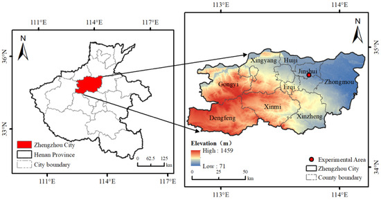
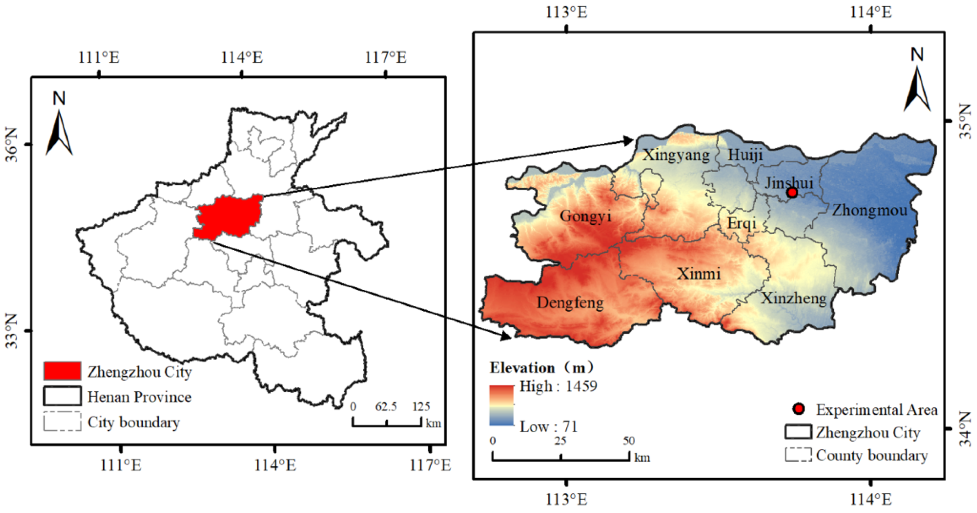
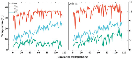
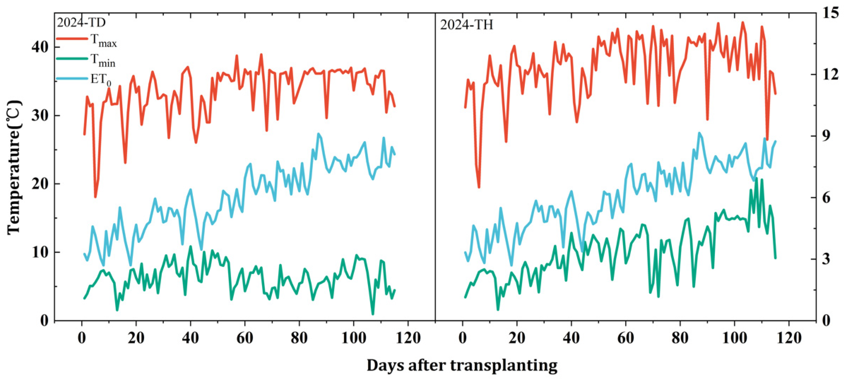
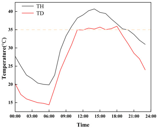
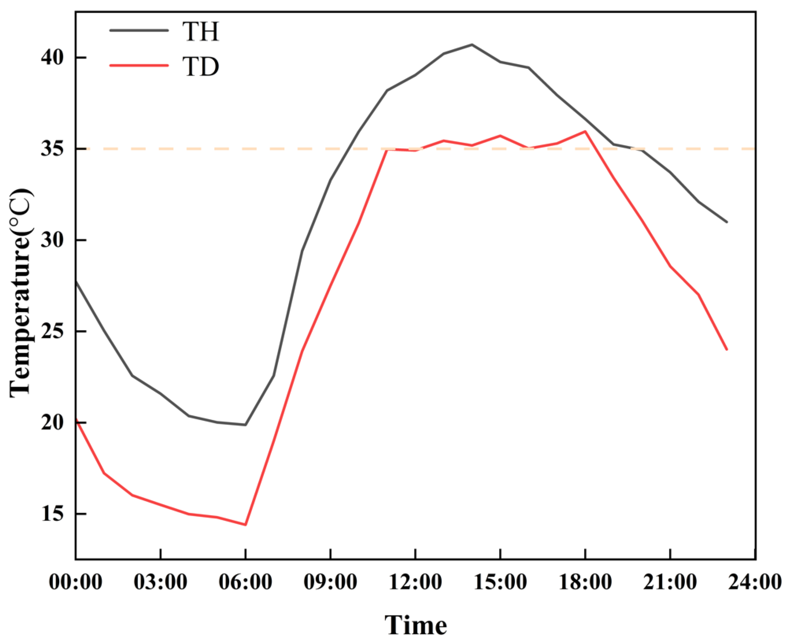
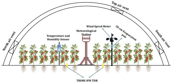
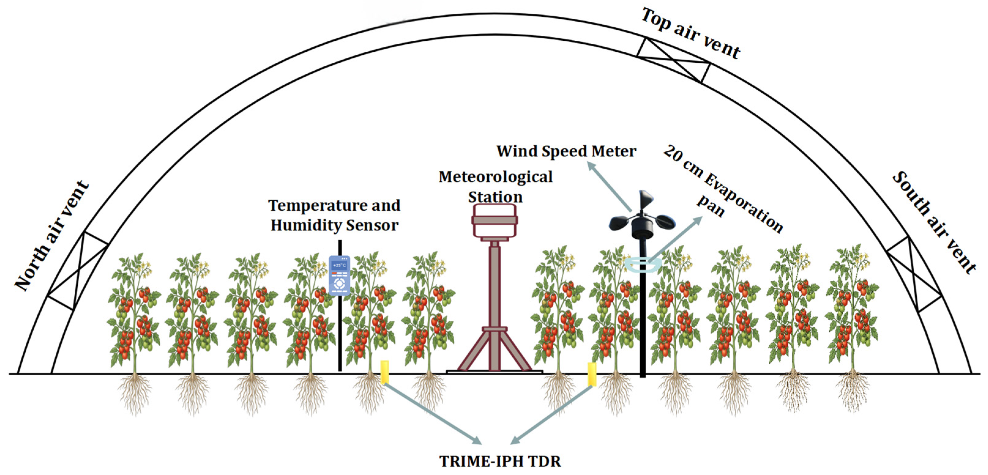
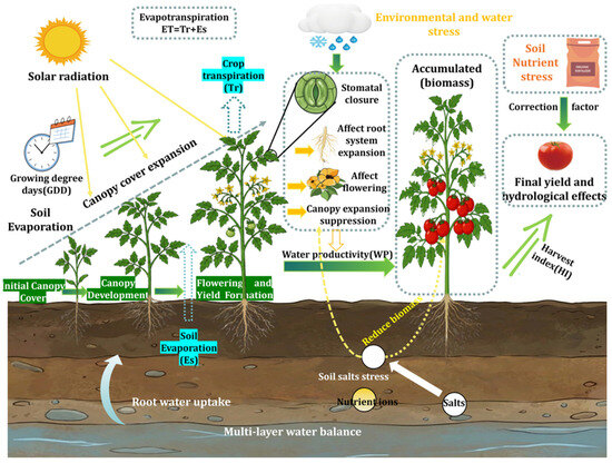
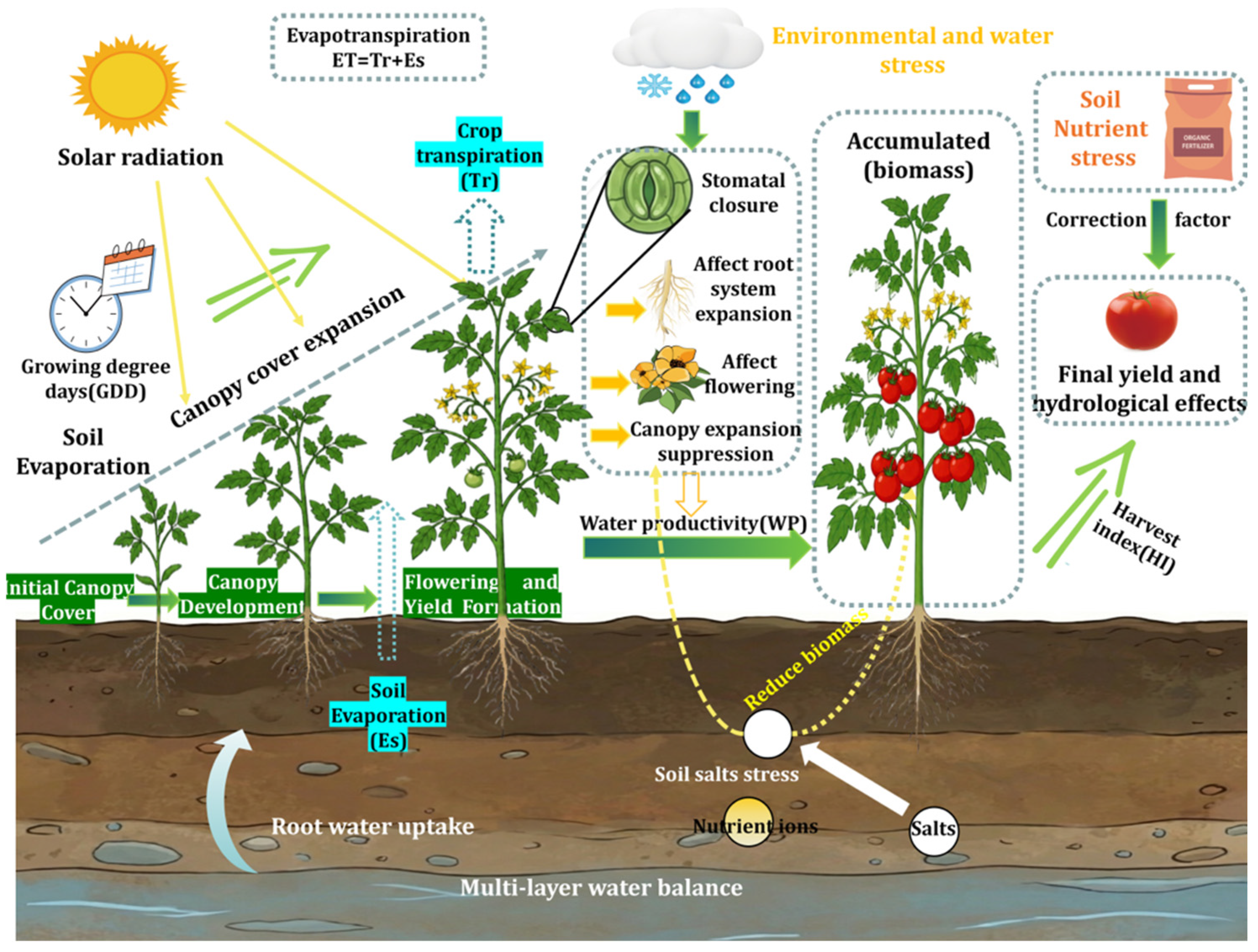
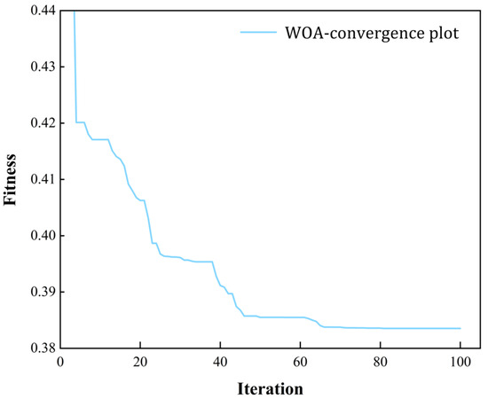
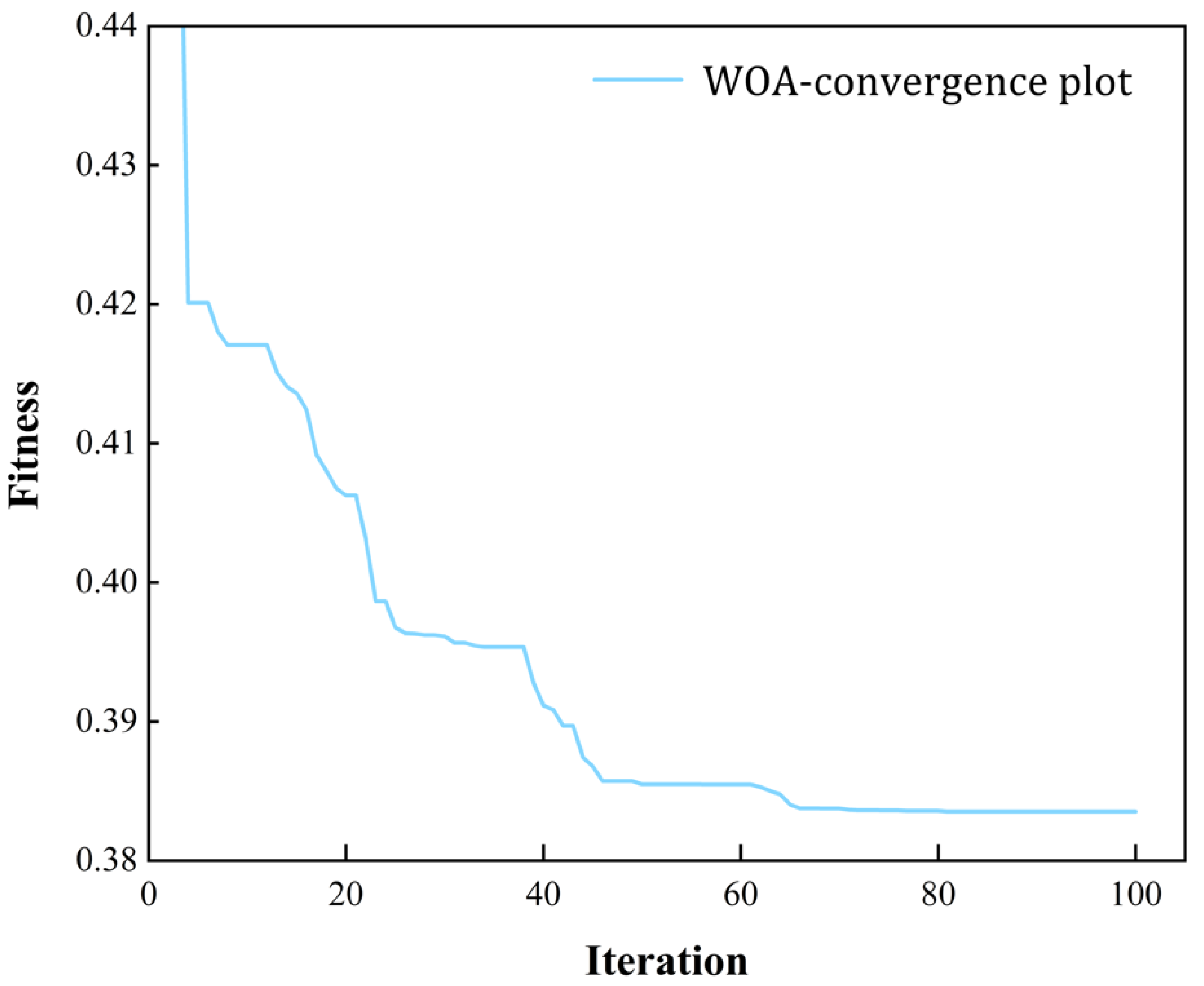
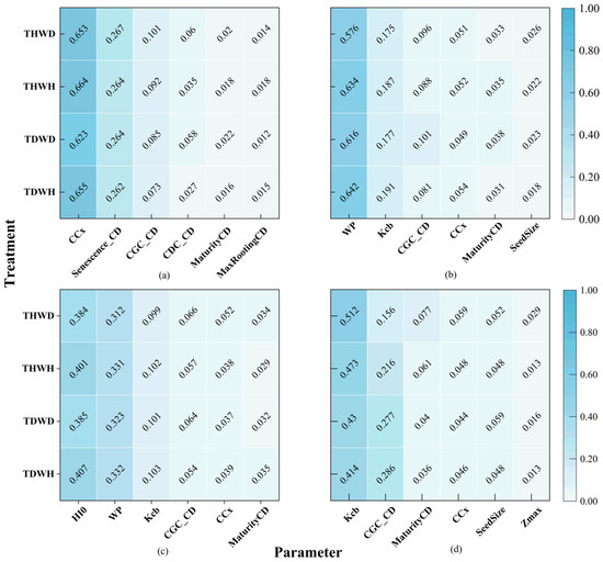
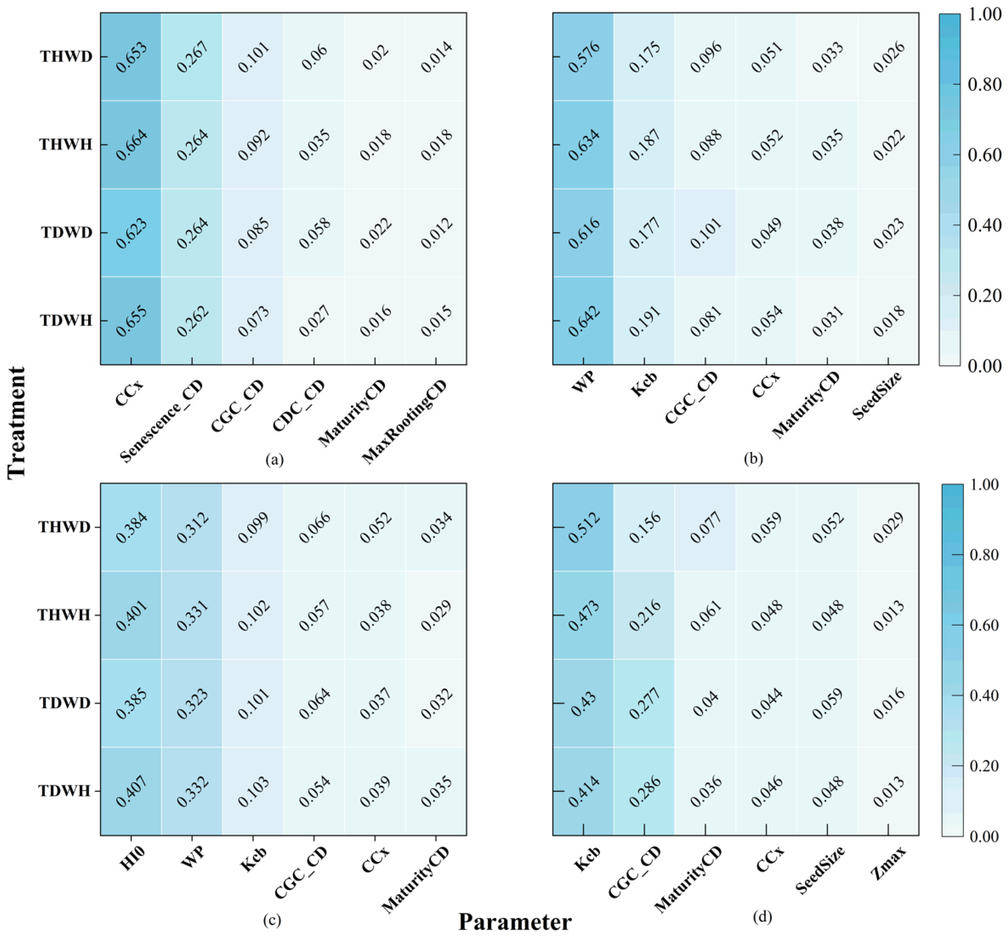
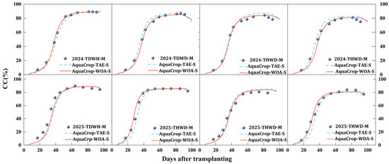
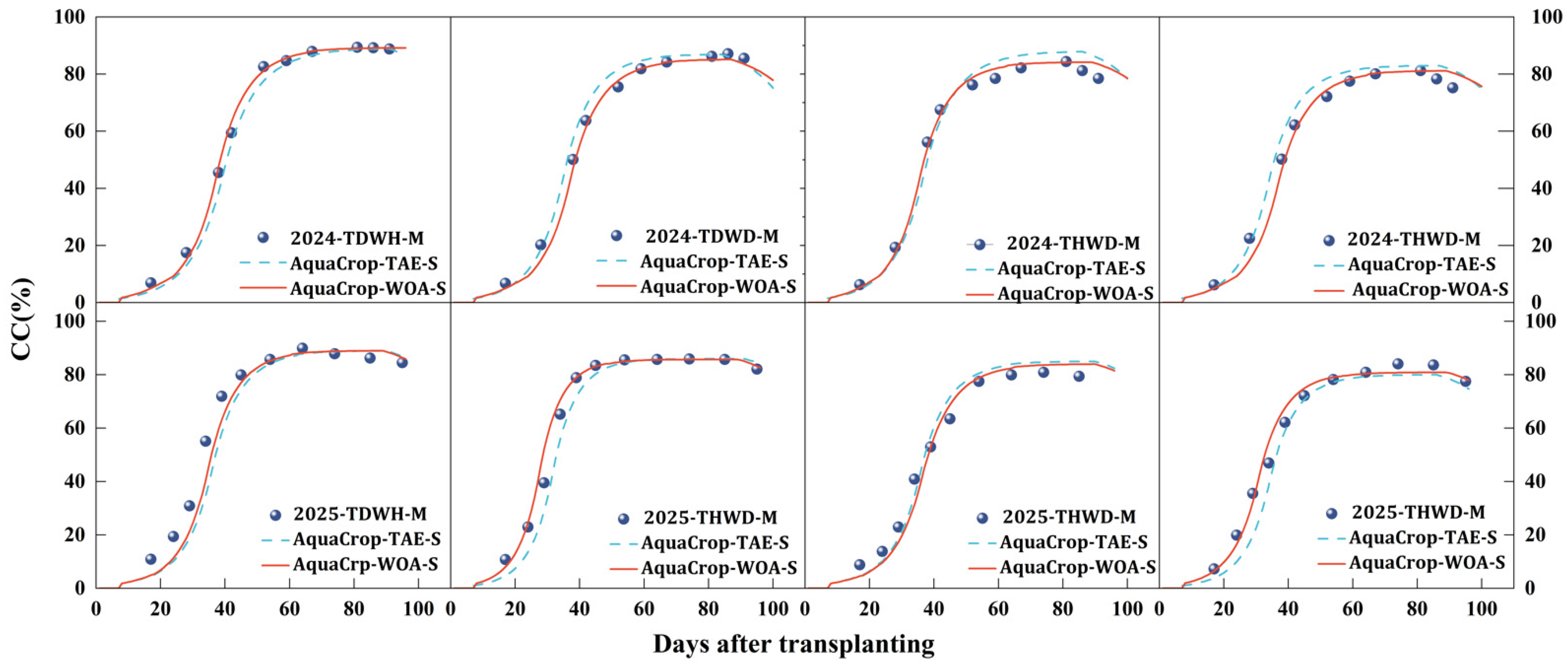
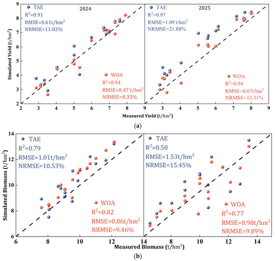
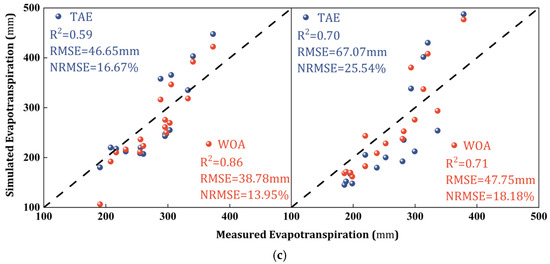
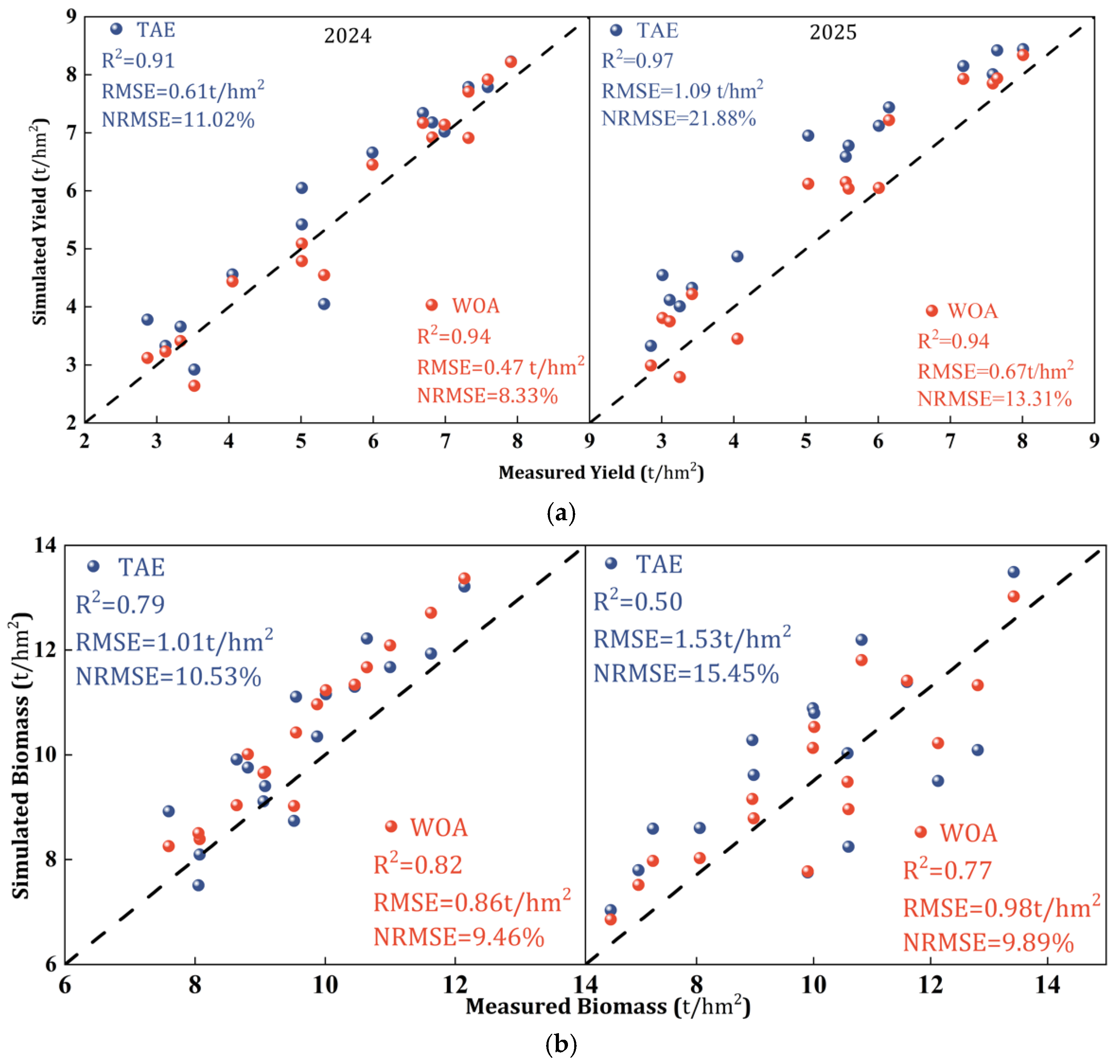
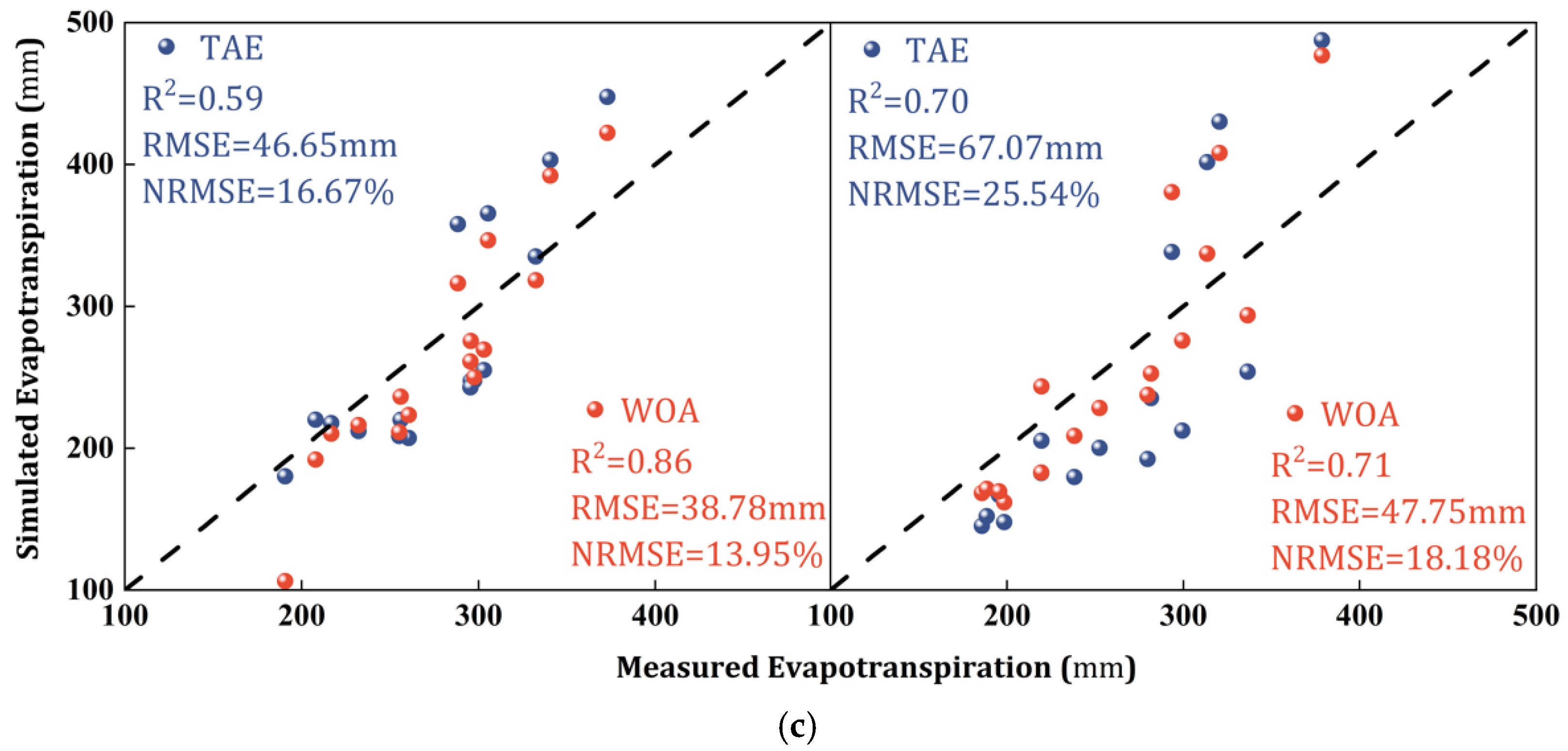

Disclaimer/Publisher’s Note: The statements, opinions and data contained in all publications are solely those of the individual author(s) and contributor(s) and not of MDPI and/or the editor(s). MDPI and/or the editor(s) disclaim responsibility for any injury to people or property resulting from any ideas, methods, instructions or products referred to in the content. |
© 2026 by the authors. Licensee MDPI, Basel, Switzerland. This article is an open access article distributed under the terms and conditions of the Creative Commons Attribution (CC BY) license.