
LES of Particle-Laden Flow in Sharp Pipe Bends with Data-Driven Predictions of Agglomerate Breakage by Wall Impacts


Abstract
:1. Introduction
2. Euler-Lagrange Simulation Methodology
2.1. Description of the Continuous Phase
2.2. Description of the Disperse Phase
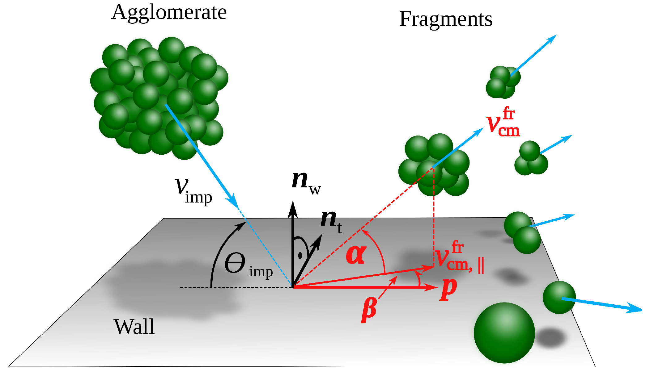
3. Wall-Impact Breakage Model
3.1. DEM Wall-Impact Database
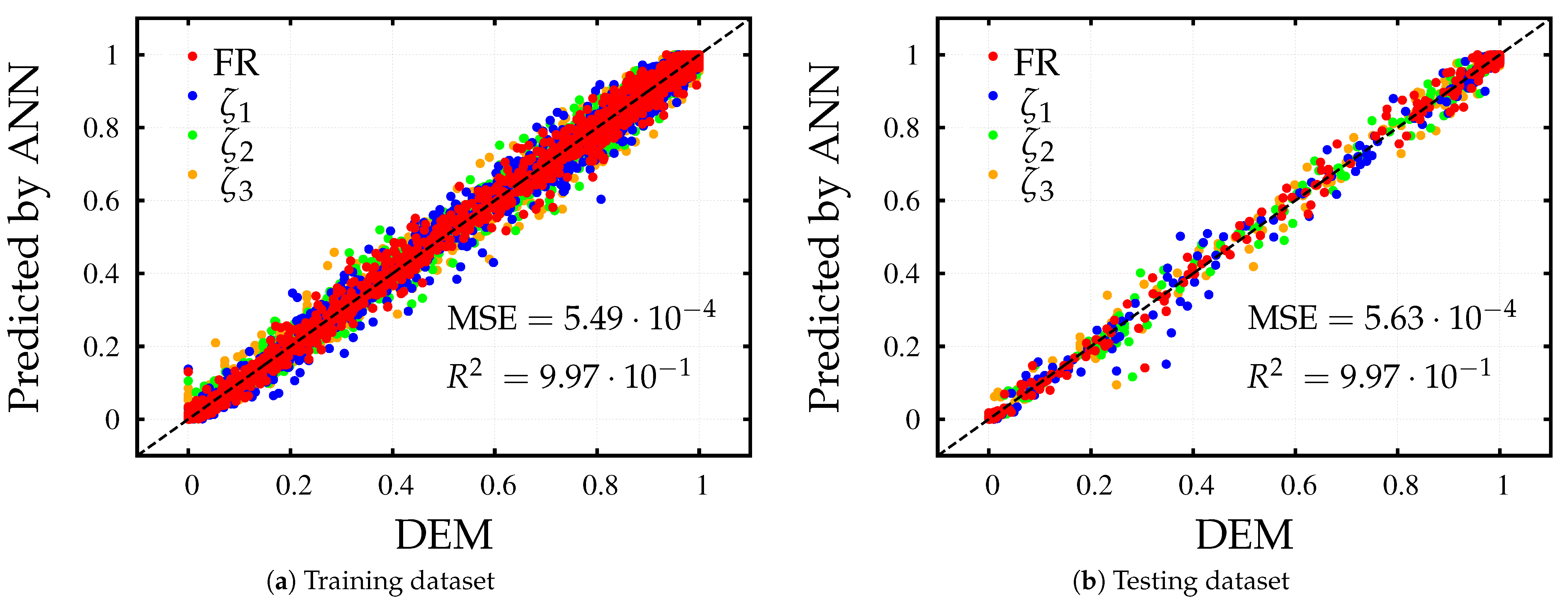
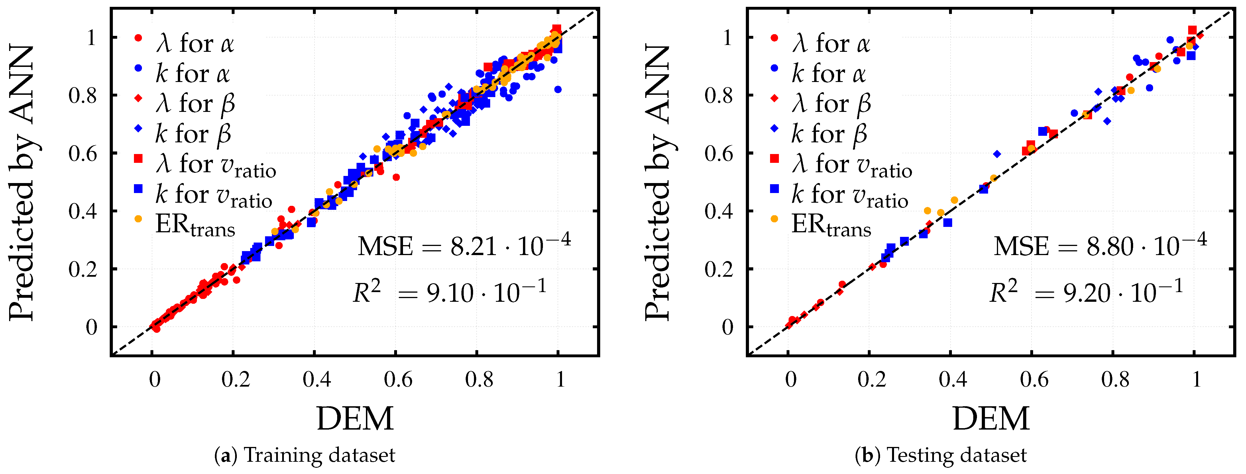
3.2. Regression by Neural Networks
4. Definition of the Setup: Particle-Laden Flow through Pipe Bends
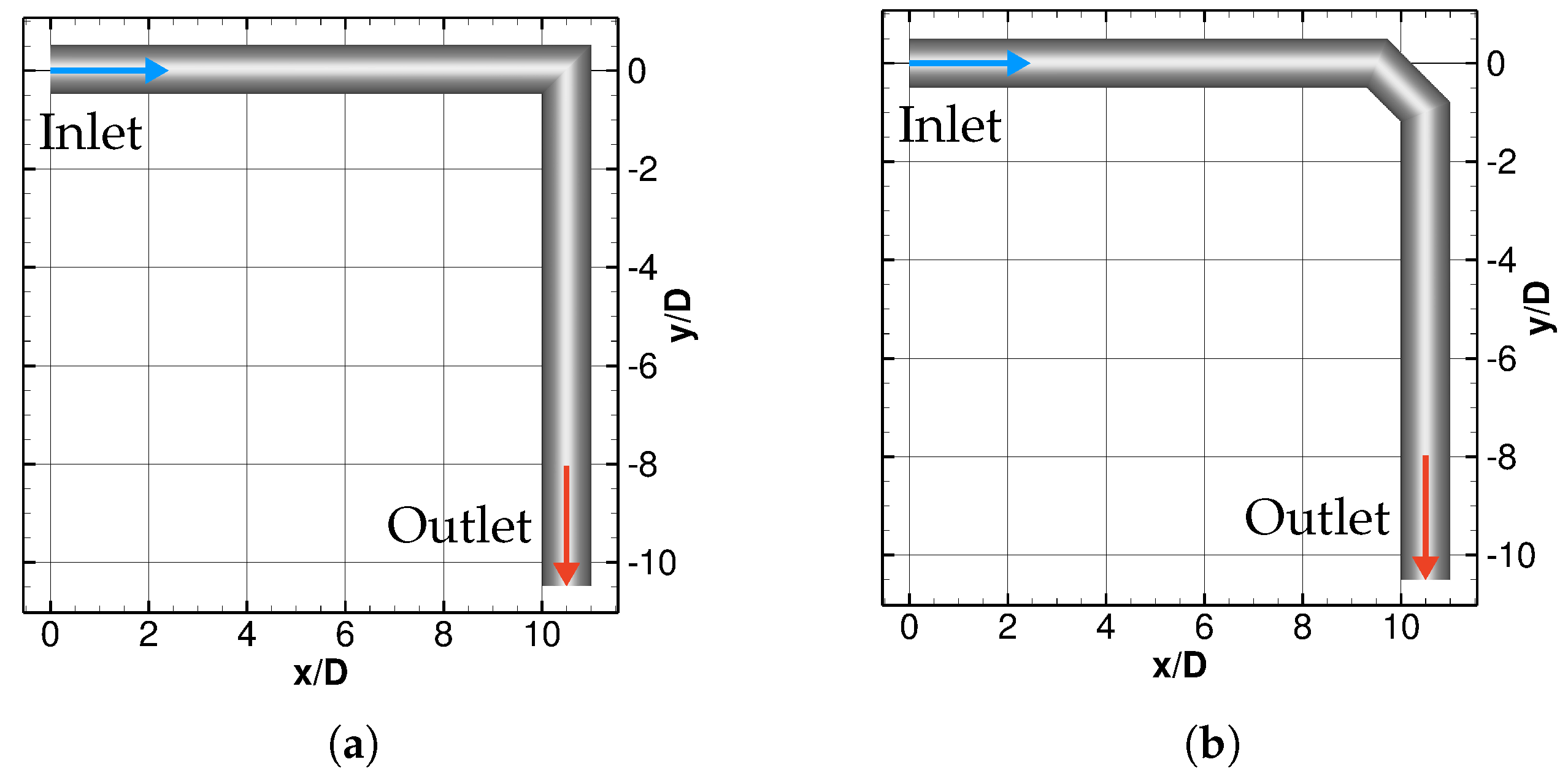
4.1. Flow Configuration
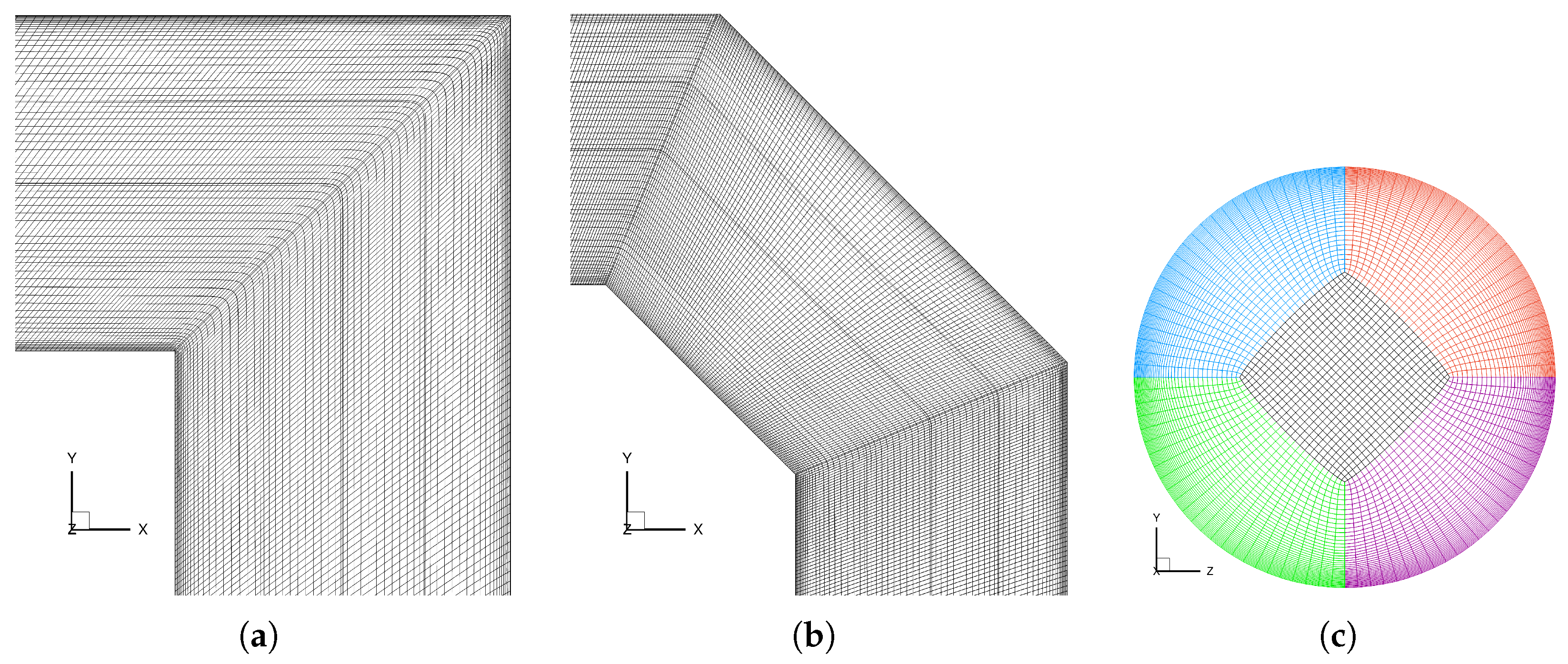
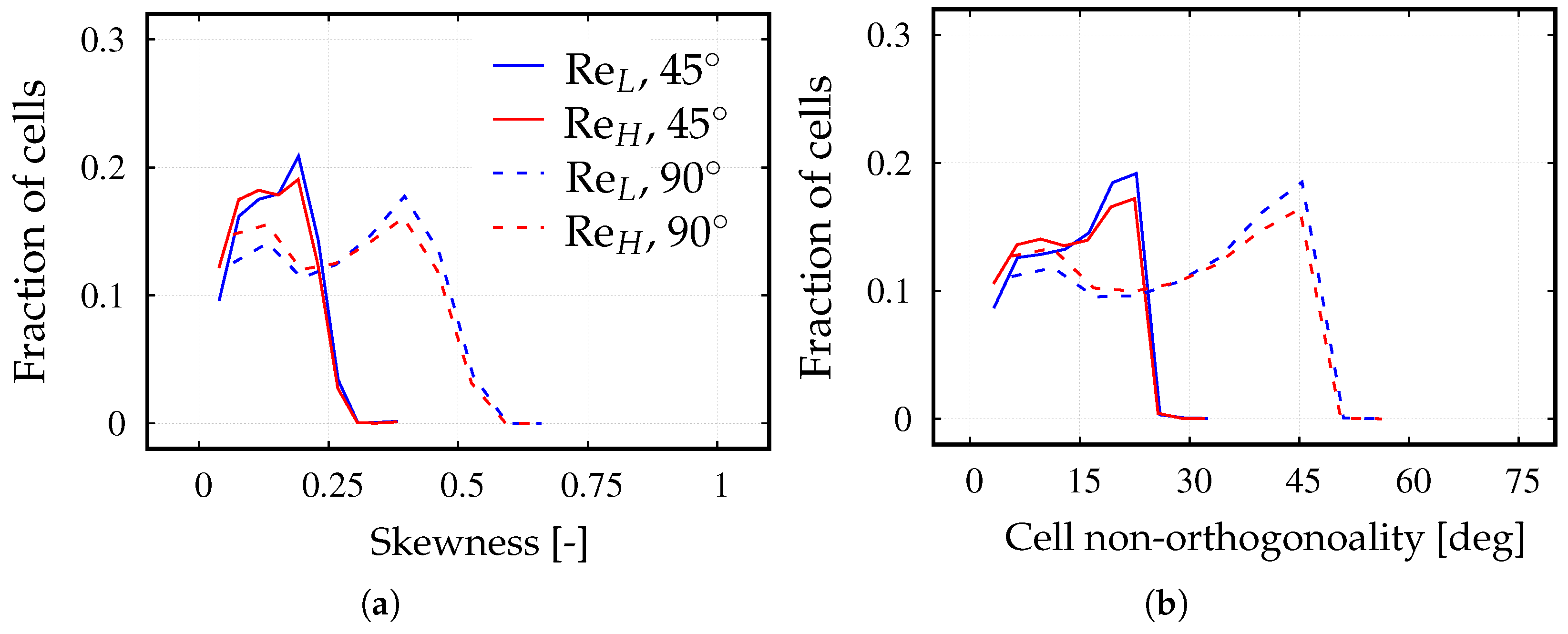
4.2. Computational Setup for the Fluid Flow
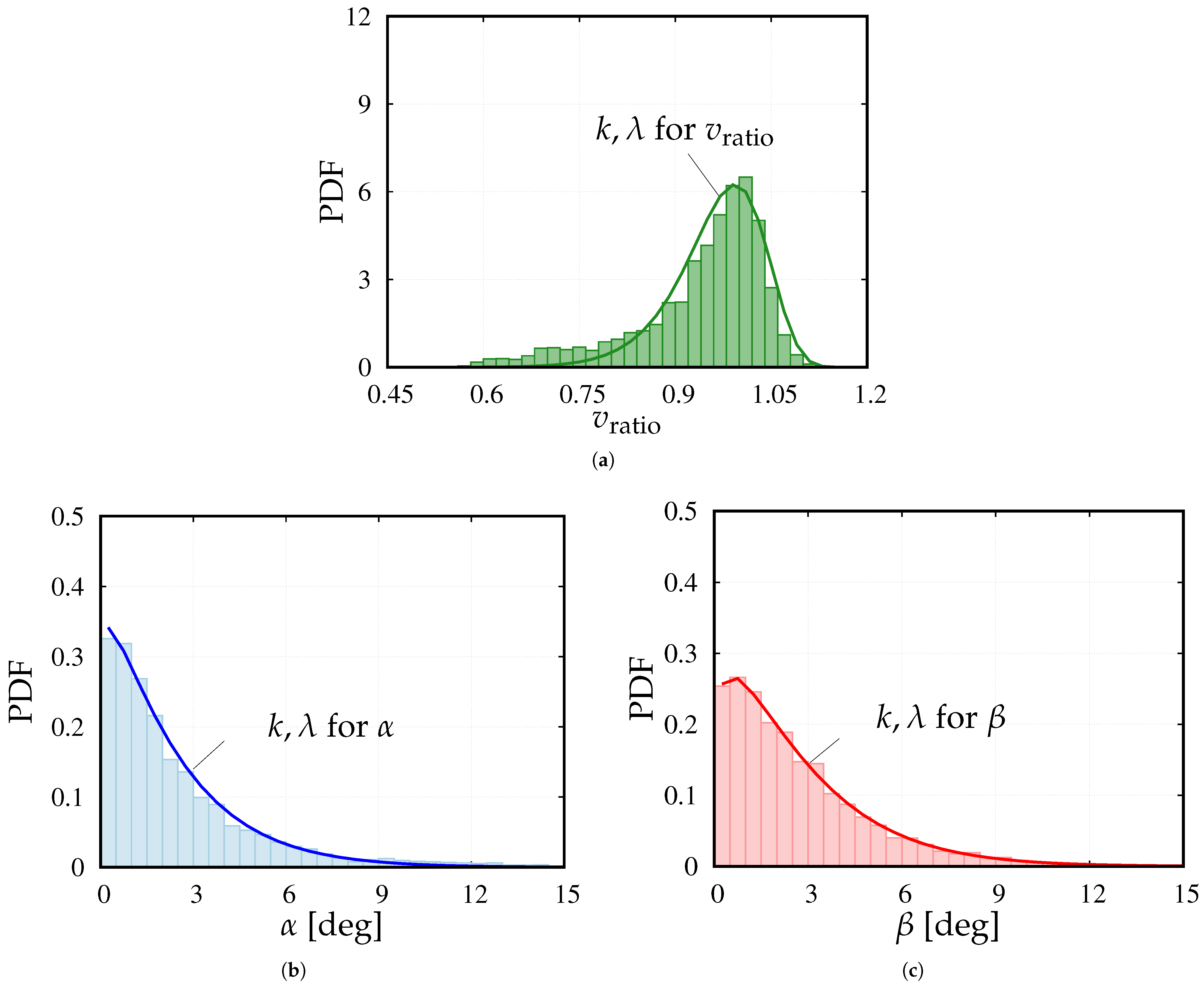
4.3. Properties of the Agglomerates
4.4. Simulation Procedure
5. Results and Discussion
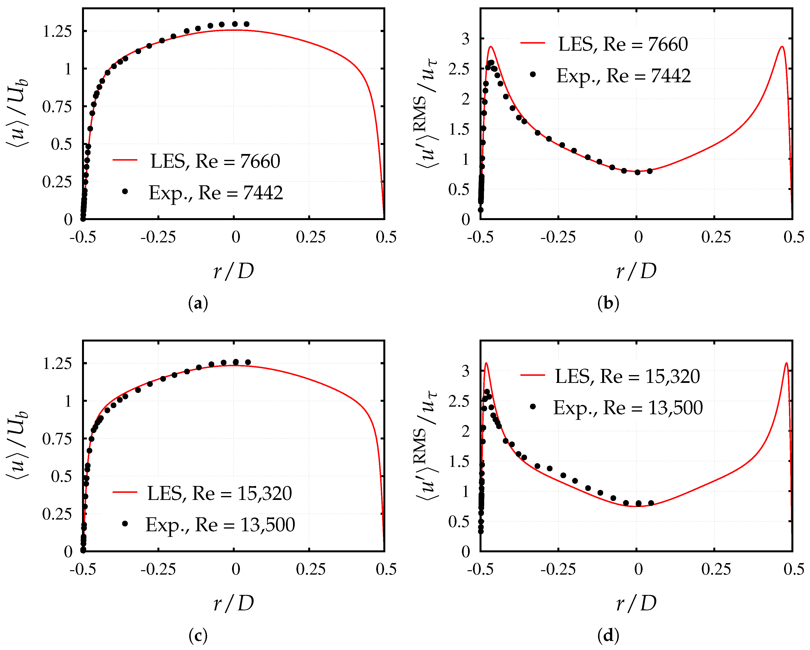
5.1. Validation of the Inflow Data
5.2. Fluid Flow in Pipe Bends
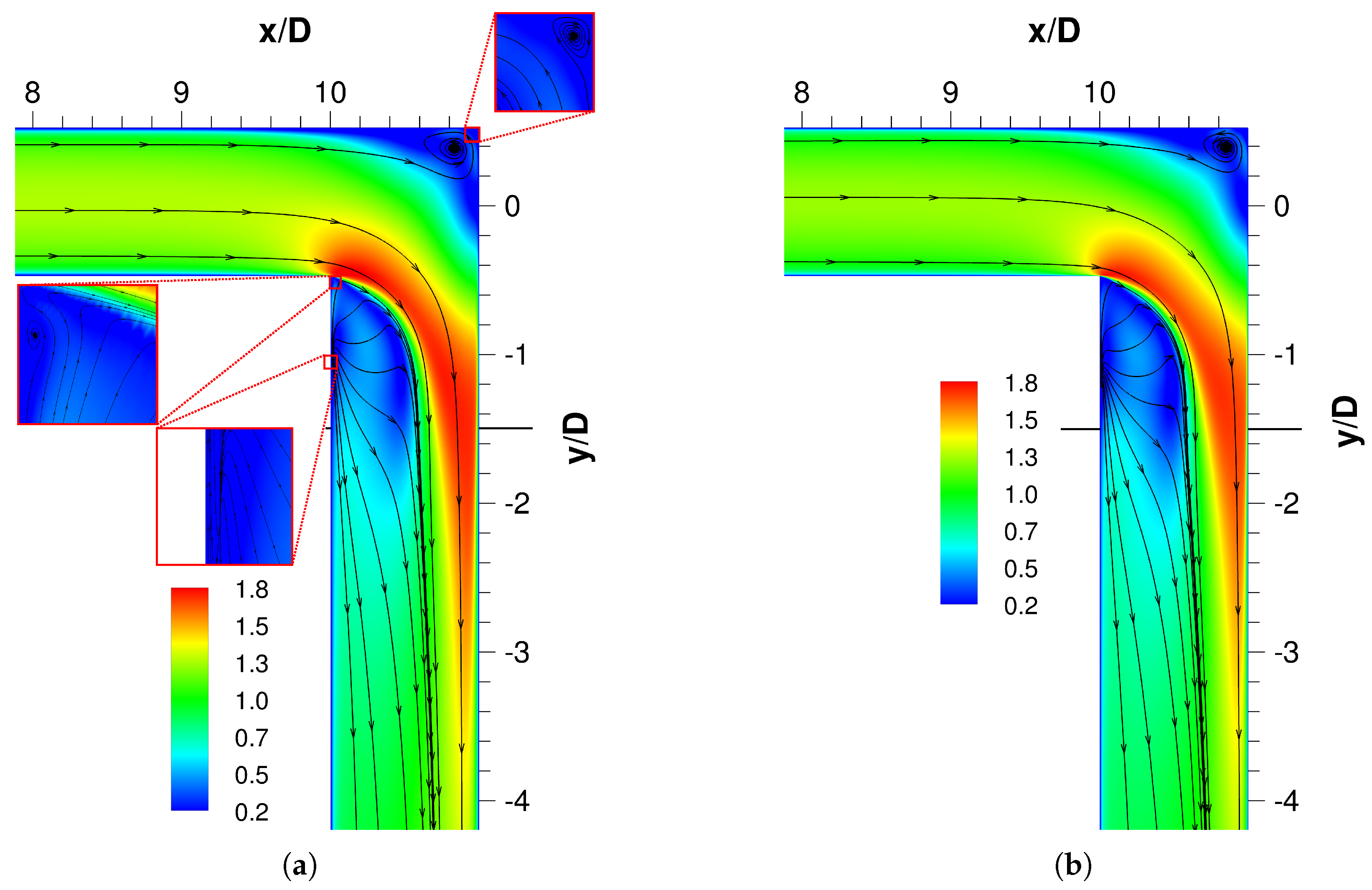
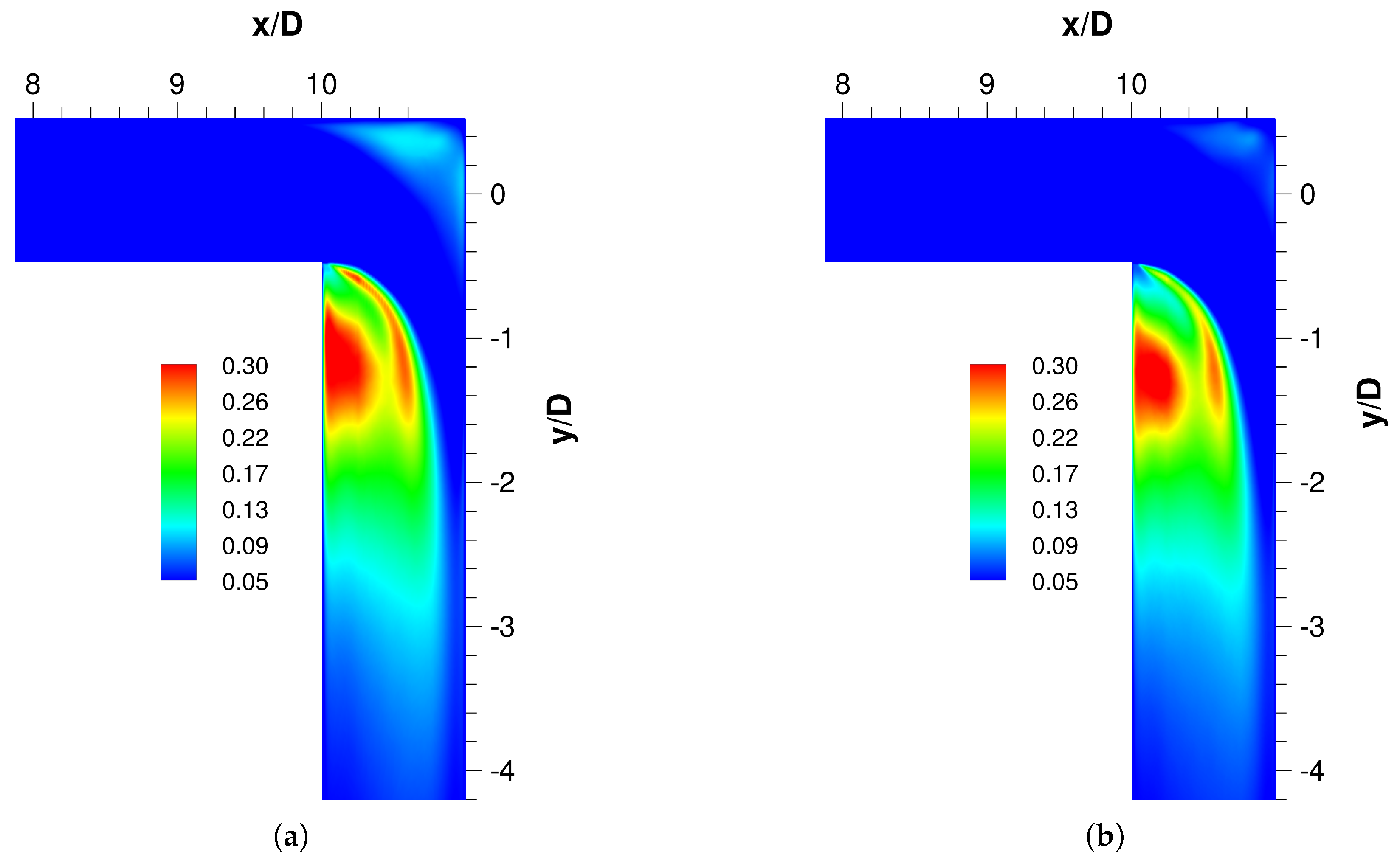
5.2.1. Flow in the 90 Pipe Bend
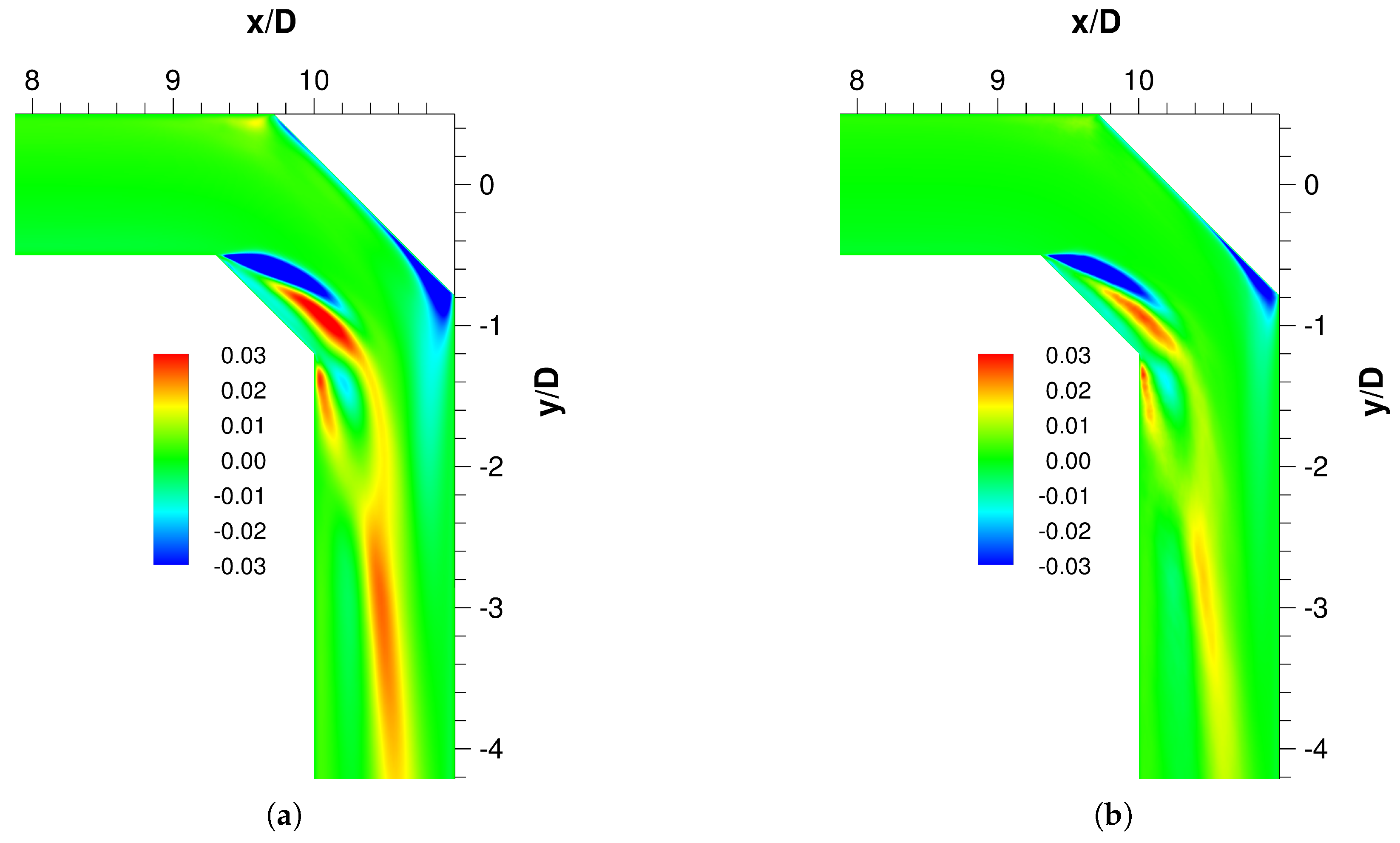
5.2.2. Flow in the 45 Pipe Bend
5.3. Breakage of Agglomerates
6. Conclusions
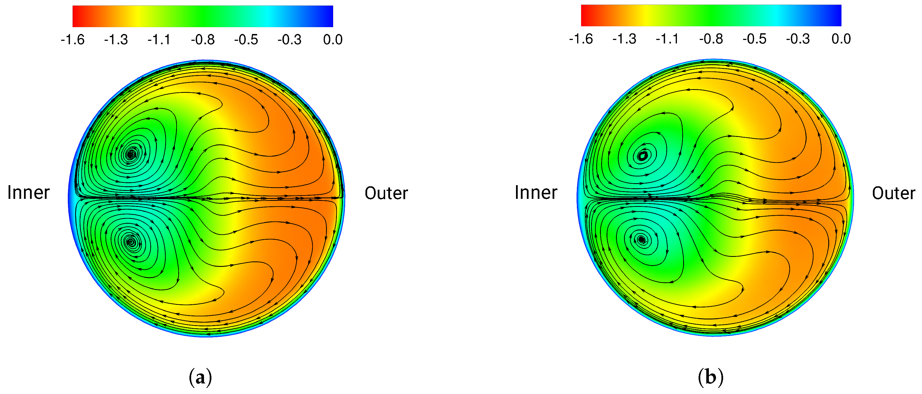
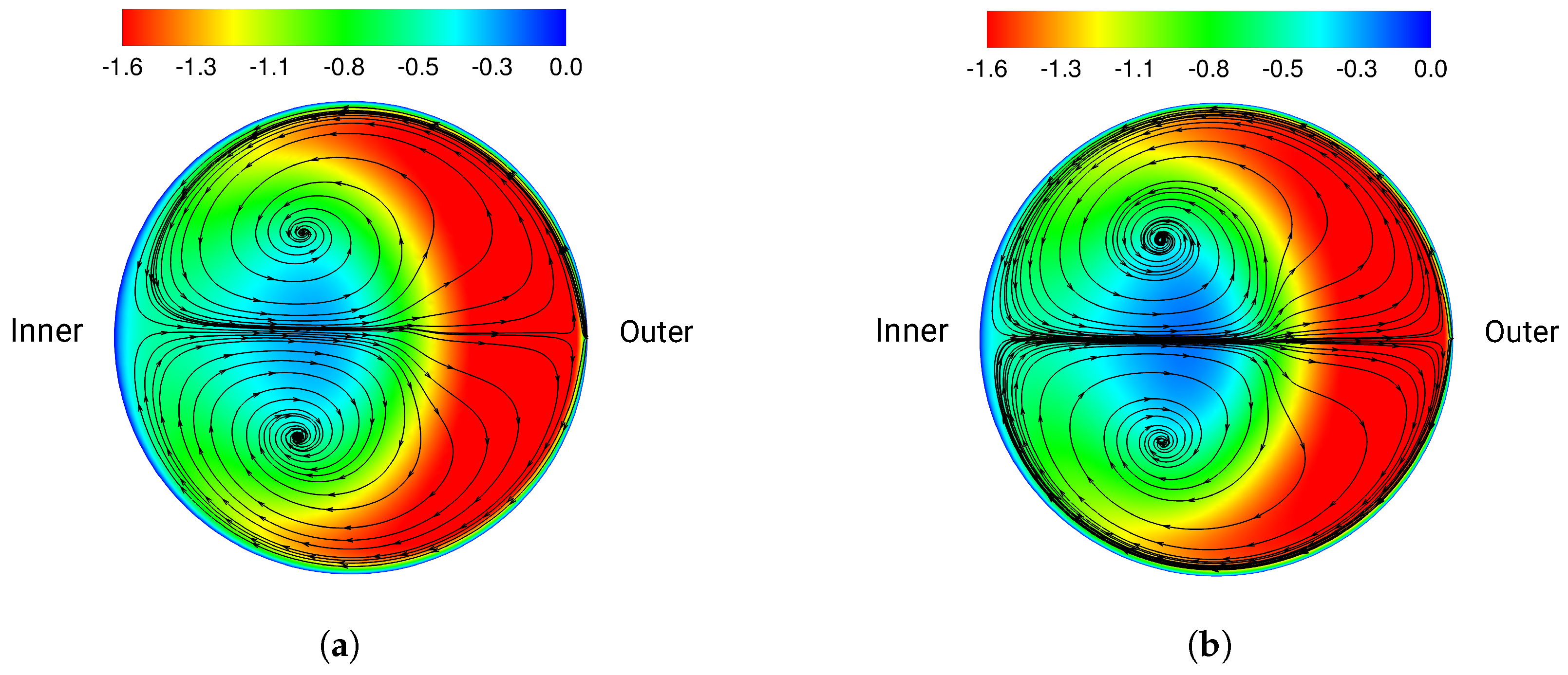
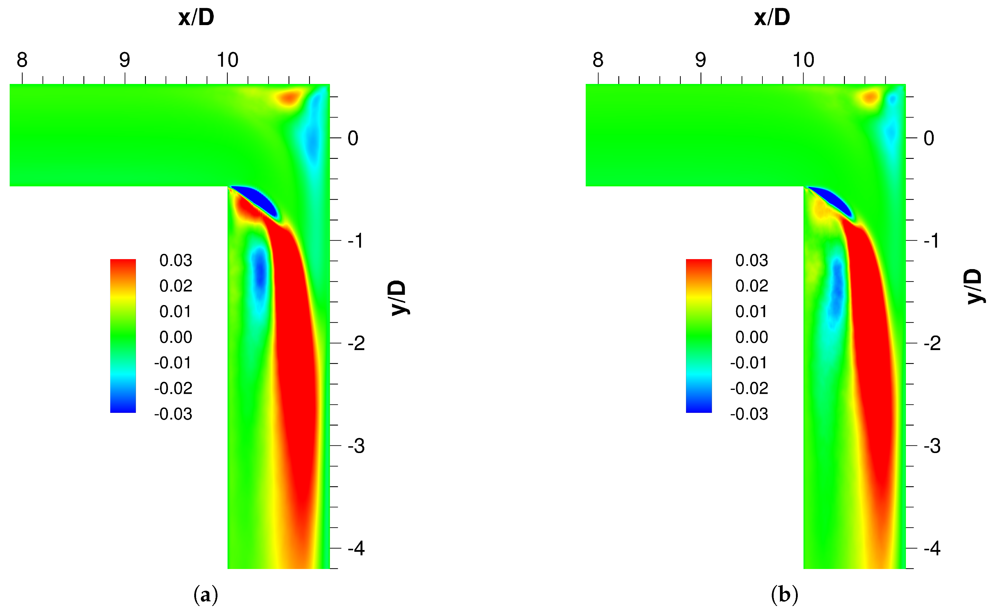
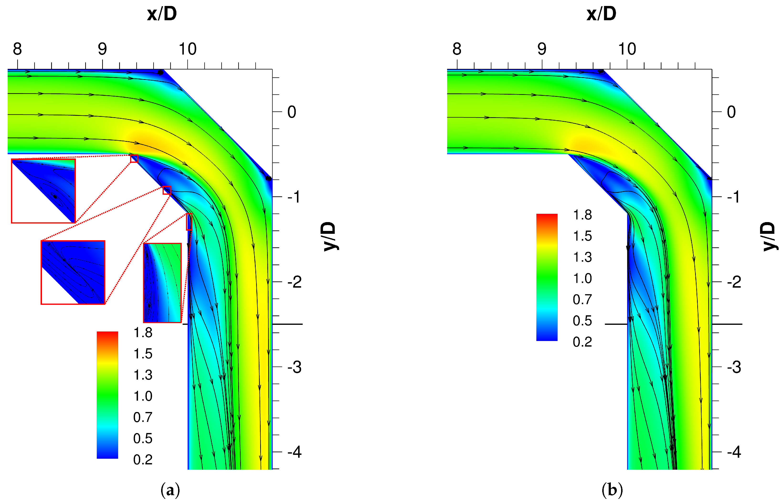
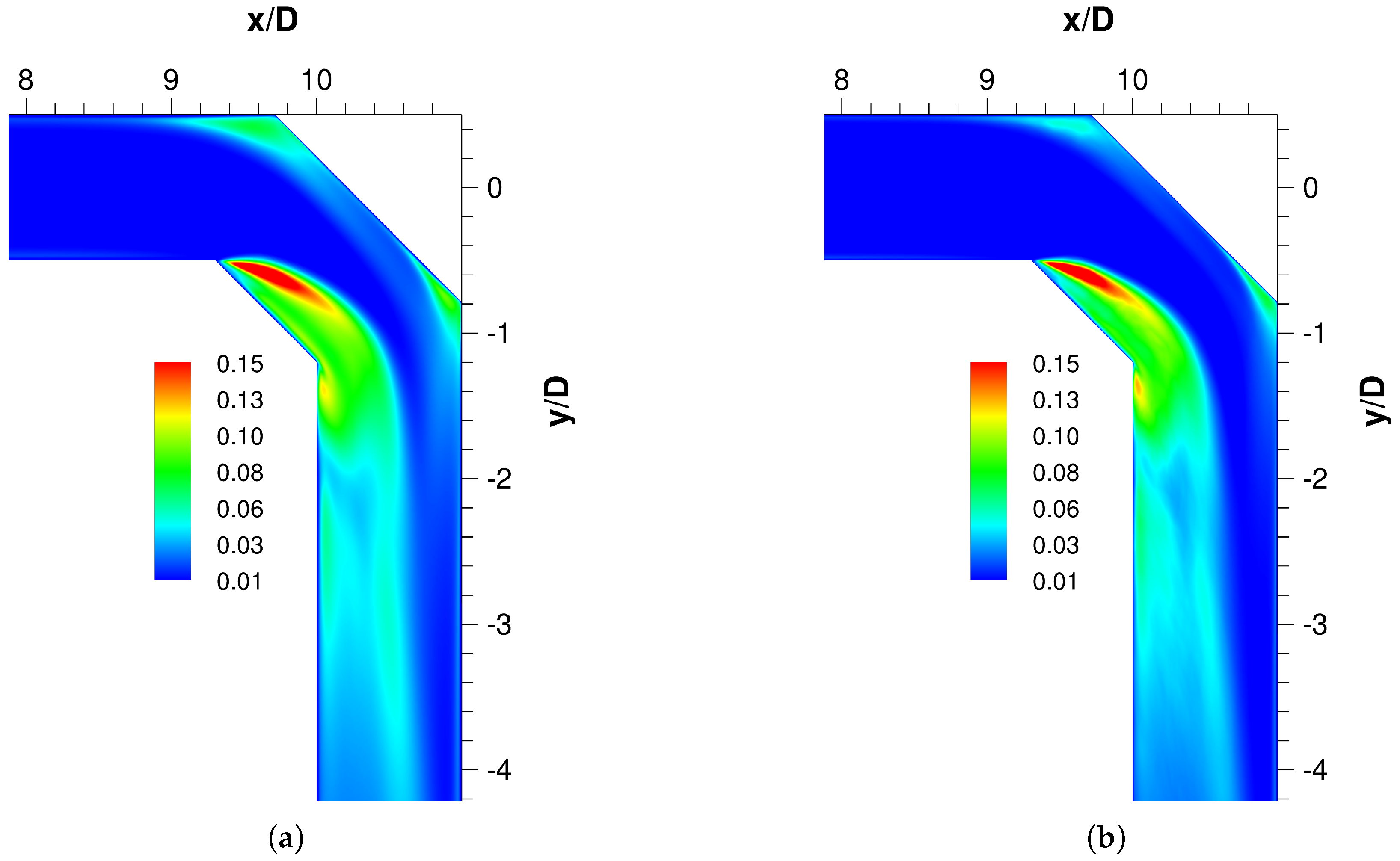
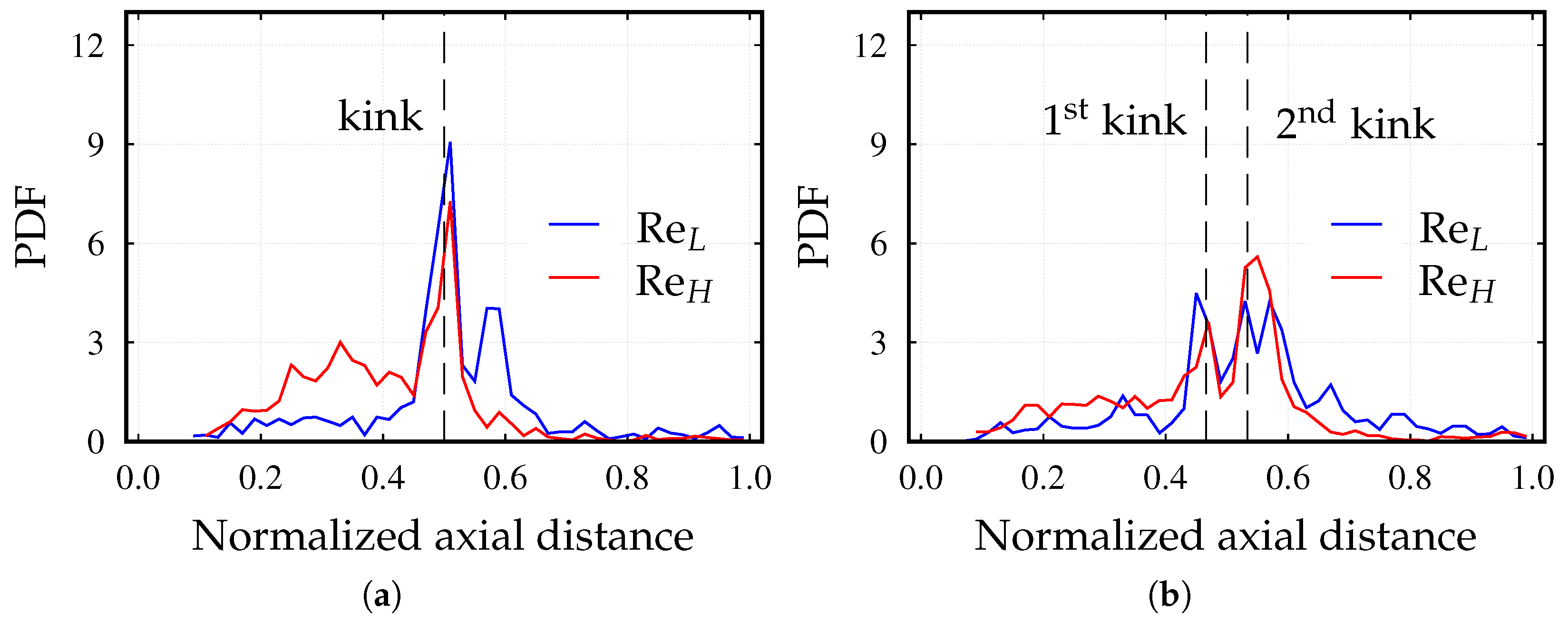
- The flow in sharp pipe bends is mainly characterized by separation zones at the kinks of the bends and secondary flow structures known as Dean vortices. The presence of the separation regions accelerates the flow in the core of the bend. The abrupt deflection of the flow direction in the 90 bend leads to large separation regions, high velocities, and strong turbulent fluctuations. The two-step deflection of the flow in the 45 bend results in weaker flow conditions.
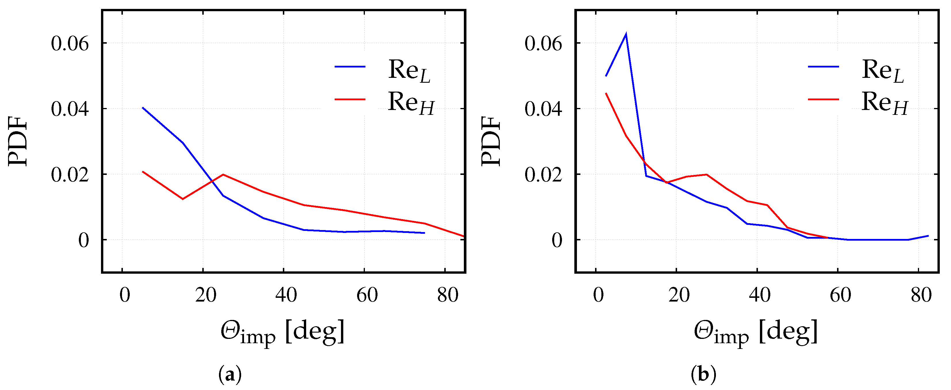
- In all four investigated configurations (two geometries and two Reynolds numbers) deagglomeration is mainly attributed to the wall-impact breakage followed by the breakage due to rotation. Other fluid-induced stress mechanisms such as drag and turbulence are found to be irrelevant under the considered, rather low Reynolds numbers. The same finding was reported by Tong et al. [10] who studied the breakage of agglomerates employing the same pipe geometries and flow Reynolds numbers, albeit different particle properties. The geometry of the bend pipes also contribute to this circumstance, since breakage by wall impactions is promoted by the sharp kink before agglomerates reach the regions of high flow shear.
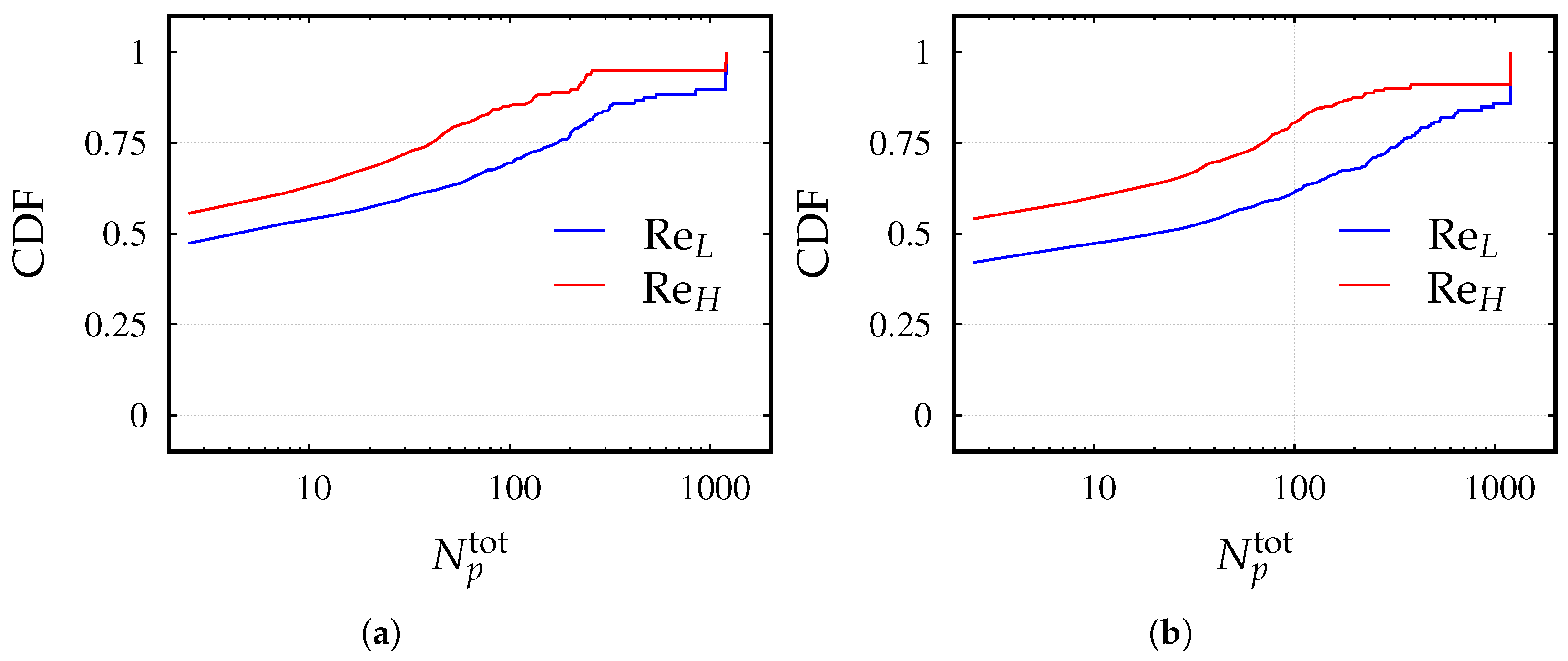
- In any of the two investigated bend geometries, increasing Re enhances breakage and leads to finer particle size distributions at the outlet of the pipe.
- Considering the same Re number, more breakage takes place in the 45 than in the 90 pipe bend. This is attributed to the favorable agglomeration conditions in the 45 case leading to more re-agglomerations and thus a higher breakage possibility. However, concentrating on the outlet of the pipe, a better deagglomeration performance is attained by the 90 bend. This is perceptible from the higher primary particle fractions in Table 3 and the finer agglomerate size distributions at the outlet of the 90 bends (see Figure 19).
Author Contributions
Funding
Institutional Review Board Statement
Informed Consent Statement
Data Availability Statement
Conflicts of Interest
Abbreviations
| ANN | Artificial neural network |
| BR | Bayesian regularization |
| CDF | Cumulative distribution function |
| CPU | Central processor unit |
| DEM | Discrete element method |
| DPI | Dry Powder Inhaler |
| ER | Energy ratio |
| FPF | Fine particle fraction |
| FR | Fragmentation ratio |
| LES | Large-eddy simulation |
| Probability distribution function | |
| PPF | Primary particle fraction |
| MPI | Message passing interface |
| MSE | Mean square error |
| RMS | Root mean squared |
References
- Darquenne, C. Aerosol deposition in health and disease. J. Aerosol. Med. Pulm. Drug Deliv. 2012, 25, 140–147. [Google Scholar] [CrossRef] [Green Version]
- Longest, P.W.; Son, Y.J.; Holbrook, L.; Hindle, M. Aerodynamic factors responsible for the deaggregation of carrier-free drug powders to form micrometer and submicrometer aerosols. Pharm. Res. 2013, 30, 1608–1627. [Google Scholar] [CrossRef] [PubMed] [Green Version]
- Chew, N.Y.K.; Chan, H.K. Influence of particle size, air flow, and inhaler device on the dispersion of mannitol powders as aerosols. Pharm. Res. 1999, 16, 1098–1103. [Google Scholar] [CrossRef] [PubMed]
- Coates, M.S.; Fletcher, D.F.; Chan, H.K.; Raper, J.A. Effect of design on the performance of a dry powder inhaler using computational fluid dynamics. Part 1: Grid structure and mouthpiece length. J. Pharm. Sci. 2004, 93, 2863–2876. [Google Scholar] [CrossRef] [PubMed]
- Adi, S.; Tong, Z.; Chan, H.K.; Yang, R.; Yu, A. Impact angles as an alternative way to improve aerosolisation of powders for inhalation? Eur. J. Pharm. Sci. 2010, 41, 320–327. [Google Scholar] [CrossRef]
- Coates, M.S.; Chan, H.K.; Fletcher, D.F.; Raper, J.A. Effect of design on the performance of a dry powder inhaler using computational fluid dynamics. Part 2: Air inlet size. J. Pharm. Sci. 2006, 95, 1382–1392. [Google Scholar] [CrossRef]
- Longest, W.; Farkas, D.; Bass, K.; Hindle, M. Use of computational fluid dynamics (CFD) dispersion parameters in the development of a new DPI actuated with low air volumes. Pharm. Res. 2019, 36, 1–17. [Google Scholar] [CrossRef]
- Wong, W.; Fletcher, D.F.; Traini, D.; Chan, H.K.; Young, P.M. The use of computational approaches in inhaler development. Adv. Drug Deliv. Rev. 2012, 64, 312–322. [Google Scholar] [CrossRef] [PubMed]
- Tong, Z.B.; Yang, R.Y.; Chu, K.W.; Yu, A.B.; Adi, S.; Chan, H.K. Numerical study of the effects of particle size and polydispersity on the agglomerate dispersion in a cyclonic flow. Chem. Eng. J. 2010, 164, 432–441. [Google Scholar] [CrossRef]
- Tong, Z.B.; Adi, S.; Yang, R.Y.; Chan, H.K.; Yu, A.B. Numerical investigation of the de-agglomeration mechanisms of fine powders on mechanical impaction. J. Aerosol Sci. 2011, 42, 811–819. [Google Scholar] [CrossRef]
- van Wachem, B.; Thalberg, K.; Remmelgas, J.; Niklasson-Björn, I. Simulation of dry powder inhalers: Combining micro-scale, meso-scale and macro-scale modeling. AIChE J. 2017, 63, 501–516. [Google Scholar] [CrossRef] [Green Version]
- Crowe, C.T.; Sommerfeld, M.; Tsuji, Y. Multiphase Flows with Droplets and Particles; CRC Press: Boca Raton, FL, USA, 1998. [Google Scholar]
- Breuer, M.; Alletto, M. Efficient simulation of particle–laden turbulent flows with high mass loadings using LES. Int. J. Heat Fluid Flow 2012, 35, 2–12. [Google Scholar] [CrossRef]
- Ho, C.A.; Sommerfeld, M. Modelling of Micro–Particle Agglomeration in Turbulent Flows. Chem. Eng. Sci. 2002, 57, 3073–3084. [Google Scholar]
- Breuer, M.; Almohammed, N. Modeling and simulation of particle agglomeration in turbulent flows using a hard–sphere model with deterministic collision detection and enhanced structure models. Int. J. Multiph. Flow 2015, 73, 171–206. [Google Scholar] [CrossRef]
- Almohammed, N.; Breuer, M. Modeling and simulation of agglomeration in turbulent particle–laden flows: A comparison between energy–based and momentum–based agglomeration models. Powder Technol. 2016, 294, 373–402. [Google Scholar] [CrossRef]
- Li, A.; Ahmadi, G. Deposition of aerosols on surfaces in a turbulent channel flow. Int. J. Eng. Sci. 1993, 31, 435–451. [Google Scholar] [CrossRef]
- Almohammed, N.; Breuer, M. Modeling and simulation of particle–wall adhesion of aerosol particles in particle–laden turbulent flows. Int. J. Multiph. Flow 2016, 85, 142–156. [Google Scholar] [CrossRef]
- Breuer, M.; Khalifa, A. Refinement of breakup models for compact powder agglomerates exposed to turbulent flows considering relevant time scales. Comput. Fluids 2019, 194, 104315. [Google Scholar] [CrossRef]
- Breuer, M.; Khalifa, A. Revisiting and improving models for the breakup of compact dry powder agglomerates in turbulent flows within Eulerian–Lagrangian simulations. Powder Technol. 2019, 348, 105–125. [Google Scholar] [CrossRef]
- Ariane, M.; Sommerfeld, M.; Alexiadis, A. Wall collision and drug-carrier detachment in dry powder inhalers: Using DEM to devise a sub-scale model for CFD calculations. Powder Technol. 2018, 334, 65–75. [Google Scholar] [CrossRef]
- van Wachem, B.; Thalberg, K.; Nguyen, D.; de Juan, L.M.; Remmelgas, J.; Niklasson-Bjorn, I. Analysis, modelling and simulation of the fragmentation of agglomerates. Chem. Eng. Sci. 2020, 227, 115944. [Google Scholar] [CrossRef]
- Khalifa, A.; Breuer, M. An efficient model for the breakage of agglomerates by wall impact applied to Euler-Lagrange LES predictions. Int. J. Multiph. Flow 2021, 142, 103625. [Google Scholar] [CrossRef]
- Khalifa, A.; Breuer, M.; Gollwitzer, J. Neural-network based approach for modeling wall-impact breakage of agglomerates in particle-laden flows applied in Euler-Lagrange LES. Int. J. Heat Fluid Flow 2021. [Google Scholar] [CrossRef]
- Alletto, M.; Breuer, M. One–way, two–way and four–way coupled LES predictions of a particle–laden turbulent flow at high mass loading downstream of a confined bluff body. Int. J. Multiph. Flow 2012, 45, 70–90. [Google Scholar] [CrossRef]
- Breuer, M. Large–eddy simulation of the sub–critical flow past a circular cylinder: Numerical and modeling aspects. Int. J. Numer. Meth. Fluids 1998, 28, 1281–1302. [Google Scholar] [CrossRef]
- Breuer, M. A challenging test case for large–eddy simulation: High Reynolds number circular cylinder flow. Int. J. Heat Fluid Flow 2000, 21, 648–654. [Google Scholar] [CrossRef]
- Breuer, M. Direkte Numerische Simulation und Large–Eddy Simulation turbulenter Strömungen auf Hochleistungsrechnern; Habilitationsschrift, Universität Erlangen–Nürnberg, Berichte aus der Strömungstechnik, Shaker Verlag: Aachen, Germany, 2002. [Google Scholar]
- Rhie, C.M.; Chow, W.L. A numerical study of the turbulent flow past an isolated airfoil with trailing edge separation. AIAA J. 1983, 21, 1525–1532. [Google Scholar] [CrossRef]
- Stone, H.L. Iterative solution of implicit approximations of multidimensional partial differential equations. SIAM J. Num. Anal. 1968, 5, 530–558. [Google Scholar] [CrossRef]
- Smagorinsky, J. General circulation experiments with the primitive equations, I, The basic experiment. Mon. Weather Rev. 1963, 91, 99–165. [Google Scholar] [CrossRef]
- Crowe, C.T.; Sharma, M.P.; Stock, D.E. The Particle-Source-In-Cell (PSI-CELL) model for gas–droplet flows. Trans. ASME J. Fluids Eng. 1977, 99, 325–332. [Google Scholar] [CrossRef]
- Schiller, L.; Naumann, A. A drag coefficient correlation. VDI Z. 1933, 77, 318–320. [Google Scholar]
- Mei, R. An approximate expression for the shear lift force on a spherical particle at finite Reynolds number. Int. J. Multiph. Flow 1992, 18, 145–147. [Google Scholar] [CrossRef]
- Sommerfeld, M. Analysis of collision effects for turbulent gas–particle flow in a horizontal channel: Part I. Particle transport. Int. J. Multiph. Flow 2003, 29, 675–699. [Google Scholar] [CrossRef]
- Rubinow, S.I.; Keller, J.B. The transverse force on a spinning sphere moving in a viscous fluid. J. Fluid Mech. 1961, 11, 447–459. [Google Scholar] [CrossRef]
- Oesterlé, B.; Bui Dinh, T. Experiments on the lift of a spinning sphere in a range of intermediate Reynolds numbers. Exp. Fluids 1998, 19, 16–22. [Google Scholar] [CrossRef]
- Brennen, C.E. A Review of Added Mass and Fluid Inertial Forces; Technical Report; Naval Civil Engineering Laboratory: Port Hueneme, CA, USA, 1982. [Google Scholar]
- Kuerten, J.G.M. Point-particle DNS and LES of particle-laden turbulent flow—A state-of-the-art review. Flow Turbul. Combust. 2016, 97, 689–713. [Google Scholar] [CrossRef] [PubMed] [Green Version]
- Maxey, M.R.; Riley, J.J. Equation of motion for a small rigid sphere in a non–uniform flow. Phys. Fluids 1983, 26, 883–889. [Google Scholar] [CrossRef]
- Breuer, M.; Hoppe, F. Influence of a cost–efficient Langevin subgrid–scale model on the dispersed phase of a large–eddy simulation of turbulent bubble–laden and particle–laden flows. Int. J. Multiph. Flow 2017, 89, 23–44. [Google Scholar] [CrossRef]
- Breuer, M.; Baytekin, H.T.; Matida, E.A. Prediction of aerosol deposition in 90 degrees bends using LES and an efficient Lagrangian tracking method. J. Aerosol Sci. 2006, 37, 1407–1428. [Google Scholar] [CrossRef]
- Alletto, M.; Breuer, M. Prediction of turbulent particle–laden flow in horizontal smooth and rough pipes inducing secondary flow. Int. J. Multiph. Flow 2013, 55, 80–98. [Google Scholar] [CrossRef]
- Hoomans, B.P.B.; Kuipers, J.A.M.; Briels, W.J.; Van Swaaij, W.P.M. Discrete particle simulation of bubble and slug formation in a two–dimensional gas–fluidised bed: A hard–sphere approach. Chem. Eng. Sci. 1996, 51, 99–118. [Google Scholar] [CrossRef] [Green Version]
- Sommerfeld, M.; von Wachem, B.; Oliemans, R. Best Practice Guidelines for Computational Fluid Dynamics of Dispersed Multiphase Flows; ERCOFTAC: Eindhoven, UK, 2008. [Google Scholar]
- Bird, G.A. Molecular Gas Dynamics; Claredon Press: Oxford, UK, 1976. [Google Scholar]
- Harshe, Y.M.; Ehrl, L.; Lattuada, M. Hydrodynamic properties of rigid fractal aggregates of arbitrary morphology. J. Colloid Interface Sci. 2010, 352, 87–98. [Google Scholar] [CrossRef]
- Dietzel, M.; Sommerfeld, M. Numerical calculation of flow resistance for agglomerates with different morphology by the Lattice–Boltzmann Method. Powder Technol. 2013, 250, 122–137. [Google Scholar] [CrossRef]
- Dietzel, M.; Ernst, M.; Sommerfeld, M. Application of the lattice-Boltzmann method for particle-laden flows: Point-particles and fully resolved particles. Flow, Turbul. Combust. 2016, 97, 539–570. [Google Scholar] [CrossRef]
- Balachandar, S.; Moore, W.; Akiki, G.; Liu, K. Towards particle-resolved accuracy in Euler-Lagrange simulations of multiphase flow using machine learning and pairwise interaction extended point-particle (PIEP) approximation. Theor. Comput. Fluid Dyn. 2020, 34, 401–428. [Google Scholar] [CrossRef]
- Rumpf, H. The strength of granules and agglomerates. In Agglomeration; Knepper, W.A., Ed.; Interscience: New York, NY, USA, 1962; pp. 379–418. [Google Scholar]
- Khalifa, A.; Breuer, M. Data-driven model for the breakage of dry monodisperse agglomerates by wall impact applicable for multiphase flow simulations. Powder Technol. 2020, 376, 241–253. [Google Scholar] [CrossRef]
- Kloss, C.; Goniva, C.; Hager, A.; Amberger, S.; Pirker, S. Models, algorithms and validation for opensource DEM and CFD–DEM. Prog. Comput. Fluid Dyn. An. Int. J. 2012, 12, 140–152. [Google Scholar] [CrossRef]
- Hamaker, H.C. The London–van der Waals attraction between spherical particles. Physica 1937, 4, 1058–1072. [Google Scholar] [CrossRef]
- Scales, L.E. Introduction to Non-Linear Optimization; Springer: New York, NY, USA, 1985. [Google Scholar]
- MacKay, D.J.C. Bayesian interpolation. Neural Comput. 1992, 4, 415–447. [Google Scholar] [CrossRef]
- Hagan, M.; Demuth, H.; Beale, M.; De Jesús, O. Neural Network Design; self-published, 2014. [Google Scholar]
- Adi, S.; Adi, H.; Chan, H.K.; Tong, Z.; Yang, R.; Yu, A. Effects of mechanical impaction on aerosol performance of particles with different surface roughness. Powder Technol. 2013, 236, 164–170. [Google Scholar] [CrossRef]
- Piomelli, U.; Chasnov, J.R. Large–eddy simulations: Theory and Applications. In Turbulence and Transition Modeling; Hallbäck, M., Henningson, D.S., Johansson, A.V., Alfredson, P.H., Eds.; Springer: Dordrecht, Netherlands, 1996; pp. 269–331. [Google Scholar]
- Moody, L.F. An approximate formula for pipe friction factors. Trans. ASME 1947, 69, 1005–1011. [Google Scholar]
- Weiler, C. Generierung Leicht Dispergierbarer Inhalationspulver Mittels Sprühtrocknung. Ph.D. Thesis, Johannes Gutenberg-Universität Mainz, Mainz, Germany, 2008. [Google Scholar]
- Kendall, K. Agglomerate strength. Powder Metall. 1988, 31, 28–31. [Google Scholar]
- Schubert, H. Handbuch der Mechanischen Verfahrenstechnik; Wiley-VCH Verlag GmbH & Co. KGaA: Weinheim, Germany, 2003. [Google Scholar]
- Krupp, H. Particle adhesion theory and experiment. Adv. Colloid Interf. Sci. 1967, 1, 111–239. [Google Scholar]
- Foerster, S.F.; Louge, M.Y.; Chang, H.; Allia, K. Measurements of the collision properties of small spheres. Phys. Fluids 1994, 6, 1108–1115. [Google Scholar] [CrossRef] [Green Version]
- Azomaterials.com. Silica—Silicon Dioxide (SiO2). Available online: https://www.azom.com/properties.aspx?ArticleID=1114 (accessed on 19 November 2021).
- Yang, R.Y.; Yu, A.B.; Choi, S.K.; Coates, M.S.; Chan, H.K. Agglomeration of fine particles subjected to centripetal compaction. Powder Technol. 2008, 184, 122–129. [Google Scholar] [CrossRef]
- Durst, F.; Jovanović, J.; Sender, J. LDA measurements in the near–wall region of a turbulent pipe flow. J. Fluid Mech. 1995, 295, 305–335. [Google Scholar] [CrossRef]
- Prandtl, L. Über die ausgebildete Turbulenz. Z. Für Angew. Math. Und Mech. (ZAMM) 1925, 5, 136–139. [Google Scholar] [CrossRef]
- Tunstall, M.J.; Harvey, J.K. On the effect of a sharp bend in a fully developed turbulent pipe-flow. J. Fluid Mech. 1968, 34, 595–608. [Google Scholar] [CrossRef]
- Dean, W. XVI. Note on the motion of fluid in a curved pipe. Lond. Edinb. Dublin Philos. Mag. J. Sci. 1927, 4, 208–223. [Google Scholar] [CrossRef]
- Hufnagel, L.; Canton, J.; Örlü, R.; Marin, O.; Merzari, E.; Schlatter, P. The three-dimensional structure of swirl-switching in bent pipe flow. J. Fluid Mech. 2018, 835, 86–101. [Google Scholar] [CrossRef] [Green Version]
- Bluestein, A.M.; Venters, R.; Bohl, D.; Helenbrook, B.T.; Ahmadi, G. Turbulent flow through a ducted elbow and plugged tee geometry: An experimental and numerical study. J. Fluids Eng. 2019, 141, 081101. [Google Scholar] [CrossRef]
- Arun, G.; Kumaresh Babu, S.; Natarajan, S.; Kulasekharan, N. Study of flow behaviour in sharp and mitred pipe bends. Mater. Today Proc. 2020, 27, 2101–2108. [Google Scholar] [CrossRef]
- Venters, R.; Helenbrook, B.T.; Ahmadi, G.; Bohl, D.; Bluestein, A. Flow through an elbow: A direct numerical simulation investigating turbulent flow quantities. Int. J. Heat Fluid Flow 2021, 90, 108835. [Google Scholar] [CrossRef]


| Geometry | Re | Streamwise | Cross-Section | Total |
|---|---|---|---|---|
| 90 | 7660 | 898 | 4725 | 4.2 million |
| 15,320 | 1498 | 7680 | 11.5 million | |
| 45 | 7660 | 1077 | 4725 | 5.0 million |
| 15,320 | 1637 | 7680 | 12.6 million |
| Parameter | Unit | Value |
|---|---|---|
| Primary particle diameter | m | 0.97 |
| Primary particle density | kg·m | 2000 |
| Poisson’s ratio | - | 0.17 |
| Modulus of elasticity E | N/m | |
| Hamaker constant H | J | |
| Min. inter-particle distance | m | |
| Normal restitution coefficient | - | 0.97 |
| Tangential restitution coefficient | - | 0.44 |
| Static friction coefficient | - | 0.94 |
| Kinetic friction coefficient | - | 0.092 |
| Bend | Case | Wall Impact | Rotation | PPF | ||
|---|---|---|---|---|---|---|
| [%] | [%] | [%] | ||||
| 90 | 97.0 | 3.0 | 52.8 | 289.1 | 84.7 | |
| 90 | 98.9 | 1.1 | 54.1 | 357.2 | 93.5 | |
| 45 | 98.6 | 1.4 | 69.2 | 320.1 | 75.0 | |
| 45 | 98.3 | 1.7 | 74.5 | 516.0 | 88.9 |
Publisher’s Note: MDPI stays neutral with regard to jurisdictional claims in published maps and institutional affiliations. |
© 2021 by the authors. Licensee MDPI, Basel, Switzerland. This article is an open access article distributed under the terms and conditions of the Creative Commons Attribution (CC BY) license (https://creativecommons.org/licenses/by/4.0/).
Share and Cite
Khalifa, A.; Gollwitzer, J.; Breuer, M. LES of Particle-Laden Flow in Sharp Pipe Bends with Data-Driven Predictions of Agglomerate Breakage by Wall Impacts. Fluids 2021, 6, 424. https://doi.org/10.3390/fluids6120424
Khalifa A, Gollwitzer J, Breuer M. LES of Particle-Laden Flow in Sharp Pipe Bends with Data-Driven Predictions of Agglomerate Breakage by Wall Impacts. Fluids. 2021; 6(12):424. https://doi.org/10.3390/fluids6120424
Chicago/Turabian StyleKhalifa, Ali, Jasper Gollwitzer, and Michael Breuer. 2021. "LES of Particle-Laden Flow in Sharp Pipe Bends with Data-Driven Predictions of Agglomerate Breakage by Wall Impacts" Fluids 6, no. 12: 424. https://doi.org/10.3390/fluids6120424
APA StyleKhalifa, A., Gollwitzer, J., & Breuer, M. (2021). LES of Particle-Laden Flow in Sharp Pipe Bends with Data-Driven Predictions of Agglomerate Breakage by Wall Impacts. Fluids, 6(12), 424. https://doi.org/10.3390/fluids6120424