


Abstract
This study clarifies how rarefaction-induced wall slip in a thin gas film affects the established inverse-cubic scaling law for the spatial nonuniformity of levitation pressure in a push–pull levitation stage. The levitation force in this stage is generated by the combined action of blowing and suction. The continuum-based stress description is retained, and only the wall boundary condition is changed from the no-slip condition to a first-order slip condition. Three-dimensional incompressible unsteady Stokes simulations in a thin-gap unit-cell model are combined with a lubrication-theory scaling analysis. The effects of levitation height, blowing-velocity distribution, port-radius ratio, and computational-domain width are examined systematically. The results show that wall slip has only a minor influence at relatively large levitation heights. As the levitation height decreases, however, rarefaction-induced slip increases the flow-rate conductance. Consequently, the intensity of the spatial variation in levitation pressure is systematically reduced below that predicted by the no-slip inverse-cubic scaling law. This departure is well described by a correction relation derived from the lubrication approximation and remains robust against changes in the prescribed blowing-velocity distribution and geometric conditions. These findings provide an incompressible baseline for predicting levitation-pressure nonuniformity within the nominal gap-based Knudsen-number range examined here.
1. Introduction
A push–pull levitation stage generates levitation force by combining blowing and suction and therefore differs from conventional aerostatic levitation stages [1]. In addition to the relatively gradual pressure field produced by the supply pressure, it inherently involves strong shear localized near the blowing and suction ports, three-dimensional flow structures, and spatial variations in the levitation pressure. In particular, when the levitation height is small, viscous effects become dominant within the thin clearance, while rarefaction-induced wall slip can alter the flow-rate characteristics, flow energy, and pressure fluctuations [2,3]. These effects may not be evaluated adequately using design guidelines based on conventional aerostatic levitation theory. Moreover, accurately measuring the velocity and pressure fields inside a microscale clearance is difficult in practical systems. The effects of the jet-velocity distribution, port diameter, and port layout are also difficult to separate systematically. Therefore, numerical analysis based on fluid-dynamic understanding is essential for accurately predicting the stability, stiffness, and vibration-suppression performance of push–pull levitation stages. Such analysis also supports the application of these stages to high-precision positioning systems [4].
Unlike conventional aerostatic levitation stages, which rely primarily on a positive pressure field generated by the supplied fluid, a push–pull levitation stage produces the levitation force through the combined action of blowing and suction. As a result, strong velocity gradients, local three-dimensional flow structures, and spatial variations in levitation pressure appear near the blowing and suction ports. Fundamental aspects of such push–pull levitation stages have been investigated through experiments and classical theoretical analyses, while recent studies have increasingly used numerical simulations to resolve the detailed flow structures within the narrow clearance [5]. In these simulations, unit-cell models with periodic boundary conditions have been employed to clarify the spatial variation of levitation pressure in steady flows and to identify scaling laws relating the flow energy to the levitation height [5]. In addition, numerical methods originally developed for turbulent channel-flow simulations have been adapted to this problem. Reducing the residual of the continuity equation to the level of machine precision suppresses divergence errors associated with the viscous terms. Such errors can become problematic under low-Reynolds-number and fine-grid conditions. Their suppression therefore improves the reliability of grid-dependence assessments [6,7,8,9,10]. Higher-order time-integration schemes have also improved the accuracy of levitation-pressure fluctuation evaluations [9,11]. Furthermore, the effects of horizontal motion of the levitated object on the established scaling laws have been examined. The transient flow response to stepwise changes in levitation height has also been investigated. These studies have supported attempts to construct reduced-order models and derive characteristic time constants [12]. These previous studies provide an essential basis for clarifying the fluid-dynamic characteristics specific to the push–pull configuration, which are difficult to interpret simply as an extension of conventional aerostatic levitation stages.
The inverse-cubic dependence on levitation height reported previously for the root-mean-square (RMS) spatial variation of levitation pressure provides a useful basis for characterizing pressure fluctuations in push–pull levitation stages [5]. This relation enables the sensitivity of the pressure field to changes in levitation height to be evaluated clearly. However, this scaling law was derived by treating the gas as a continuum and imposing the no-slip condition at the walls. Its applicability must therefore be re-examined when the levitation height in practical stages is further reduced [3,13,14,15]. For example, when the levitation height decreases from approximately 50 , as considered in previous studies, to the micrometer scale, the Knudsen number can exceed and approach [2]. In this range, the stress formulation of the Navier–Stokes equations does not necessarily become invalid immediately, but the reduced accuracy of the continuum approximation is likely to affect the wall boundary condition first, making the no-slip condition a potential source of error. This issue is particularly important for push–pull configurations, in which adjacent blowing and suction ports generate steep pressure gradients and local three-dimensional flows within a thin clearance. Consequently, even a slight modification of the wall boundary condition may be amplified in the spatial variation of levitation pressure. Therefore, it remains unclear whether the conventional inverse-cubic scaling law is retained in the presence of rarefaction-induced wall slip. It is also unclear how wall slip modifies the magnitude and levitation-height dependence of the spatial variation in levitation pressure. This problem is not merely a matter of selecting a boundary condition. It is directly linked to the evaluation of levitation stiffness, pressure nonuniformity, microvibration, and high-precision positioning performance and is therefore significant from a design perspective. In particular, the change in flow conductance must be quantified when only the wall boundary condition is changed from the no-slip condition to a first-order slip condition. The resulting effect on the scaling law for the RMS spatial variation of levitation pressure must also be evaluated [15,16]. Expressing the slip-induced reduction in pressure fluctuation as a deviation from predictions based on the conventional continuum approximation clarifies the valid range of the existing scaling law in the small-levitation-height regime. This provides a reliable design basis for improving the precision of push–pull levitation stages.
The objective of the present study is to examine whether the inverse-cubic scaling law identified in previous work [5] remains valid under wall-slip conditions caused by gas rarefaction. This law states that the RMS value of the spatial variation in levitation pressure is proportional to the inverse cube of the levitation height. This study also clarifies how wall slip affects the applicable range and quantitative characteristics of the scaling law. The incompressible unsteady Stokes equations are solved numerically in a thin-film unit-cell model of a push–pull levitation stage with periodic boundary conditions. The lubrication approximation is used to derive and interpret the scaling laws. The validity of the unit-cell model has been confirmed in previous studies [5]. For the wall boundary condition, first-order slip is introduced on the basis that rarefaction effects appear mainly in the vicinity of the walls over the range of levitation heights considered, whereas the contribution of second-order slip is assumed to be relatively small and is therefore neglected. This setting corresponds to a flow regime in which the continuum approximation remains applicable to the dominant fluid motion, while rarefaction effects can be represented as a modification of the wall boundary condition. On this basis, the present analysis employs a numerical code previously validated for turbulent channel-flow simulations [5] and adapts it to low-speed lubrication flows by omitting the convective terms. In addition, because the blowing-velocity distribution in practical devices is not sufficiently characterized, the dependence of levitation-pressure fluctuations and the inverse-cubic scaling law on the prescribed blowing-velocity distribution is also examined.
2. Methods
The present analysis considers the unit-cell flow that constitutes the gap flow in a push–pull levitation stage. A schematic of the computational domain is shown in Figure 1. As shown in the figure, a blowing port is located at the center of a square domain, while suction ports are placed at the four corners. The origin of the coordinate system is set at the center of the blowing port; the x and z-directions are taken in the horizontal plane, and the y-direction is taken normal to the wall. The lower and upper walls are located at and , respectively, and the domain lengths in the x- and z-directions are denoted by and , respectively. These geometrical quantities are nondimensionalized by the reference levitation height , which is set to , as in the previous study [5]. The radii of the blowing and suction ports are denoted by and , respectively. Figure 1a shows the case of . The overall gap flow in the levitation stage is formed by periodically repeating this unit cell in the horizontal directions; further details of the geometrical configuration are given in the previous study [5]. The total volumetric flow rate issued from the blowing port is set equal to that drawn into the suction ports. In the present study, the nondimensional velocity distribution imposed at the blowing port is prescribed as
where and C is a parameter that determines the shape of the blowing-velocity profile. where and C is a parameter that determines the shape of the blowing-velocity profile. The parameter ensures that the cross-sectional average of over the blowing port is equal to unity, i.e.,
Figure 1.
Computational domain and prescribed inlet velocity profiles. (a) Schematic of the unit-cell computational domain with periodic boundary conditions for a push–pull levitation stage. A blowing port is placed at the center of the domain, and suction outlets are located at the four corners. The representative geometry shown here corresponds to . (b) Radial profiles of the nondimensional inlet velocity, , prescribed at the blowing port. The top-hat profile , parabolic profile , and reference quadratic-function profile are compared.
In the previous study, was used [5], giving a top-hat-like velocity profile, as shown in Figure 1b. To examine the dependence of the computed results on the inlet velocity profile, the present study also considers the case of in addition to . For , the prescribed velocity profile is close to a quadratic distribution, as shown in Figure 1b. The Reynolds number is defined using as the characteristic velocity and as the characteristic length:
where , , and are the density, dynamic viscosity, and kinematic viscosity of the gas, respectively.
In this study, two types of wall boundary conditions are imposed: a wall-slip condition associated with gas rarefaction and the no-slip condition used in the previous study [5]. For the no-slip case [5], the tangential velocity components satisfy on the solid wall surfaces. The wall-normal velocity is set to on the upper wall and on the impermeable part of the lower wall, whereas prescribed blowing and suction velocities are imposed on the lower-wall inlet and outlet ports, respectively. In this study, the prescribed levitation height ranges from 3 to 50. When the levitation height is 3, the Knudsen number, defined as
is approximately 0.023, where , and the dimensional levitation height is varied over , corresponding to the nondimensional gap height . Here, the mean free path of air at room temperature and atmospheric pressure is taken as . Thus, when the prescribed levitation height is 3 micrometers, the Knudsen number is of the order of –. In addition to the aforementioned definition of the Knudsen number, the following quantities are defined and used in this study:
The first-order slip coefficient is set to , corresponding to a hard-sphere gas with diffuse reflection at the wall [3]. Therefore, following the previous study [3], the first-order slip condition is imposed in this study as
where u and w are the tangential velocity components and v is the wall-normal velocity component. The boundary conditions for the wall-normal velocity component at the upper and lower walls are set as follows: , on the impermeable part of the lower wall, on the blowing port, and on the suction ports. Here, , where and is the total suction-port area included in one periodic unit cell. For the computational domain, following the previous study [5], is set to 80 or 40. For the Reynolds number, the analysis is performed mainly at , as in the previous study. The port-radius ratio is also set to or , following the previous study [5].
The range of applicability of the first-order slip approximation adopted in the present study is clarified here. The dimensional levitation height is and, using , the corresponding Knudsen number is Thus, the maximum value is , and is satisfied for all computational conditions considered in the present study. Whereas the first-order slip term is of , the next neglected term is of , for which , Therefore, the second-order slip effect is treated as a higher-order correction to the first-order slip effect. For the push–pull levitation stage considered in the present study, the levitation height is not assumed to decrease to the submicrometer scale, and the minimum levitation height is of the order of several micrometers. Therefore, the conclusions of the present study are restricted to the range , , . At smaller levitation heights, increases and second-order slip effects may no longer be negligible. Such conditions are therefore outside the range of applicability of the present analysis, which employs only the first-order slip condition. The mean free path used in the present study, , is the value at room temperature and atmospheric pressure. Based on this value, and are assumed to be constant throughout the computational domain. Accordingly, the present analysis does not account for spatial variations in the mean free path or slip length associated with local pressure variations. Furthermore, because pressure in an incompressible formulation is defined only up to an additive constant and is set such that in the present study, the local absolute pressure cannot be uniquely determined from the numerical solution alone. The use of a constant slip length in the present study is an approximation introduced to isolate and evaluate the effect of changing the wall boundary condition on the established inverse-cubic scaling law while retaining the continuum-based stress description and the specified fluid properties. The effect of the local pressure reduction at the minimum levitation height considered is assessed a posteriori in a later section by taking atmospheric pressure as the reference absolute pressure.
The governing equations are the incompressible continuity equation and the Navier–Stokes equations without the convective term, namely the unsteady Stokes equations. As confirmed in the previous study [12], the magnitude of the convective term relative to the viscous term is of the order of , except near the blowing port, and is therefore treated as sufficiently small in this study. The maximum velocity in the computational domain considered in this study appears at the center of the blowing port, and the largest Mach number on this central axis under the present conditions is approximately 0.26. Although the maximum local Mach number reaches approximately 0.26 near the blowing-port centerline, the present study neglects compressibility in order to isolate the effect of wall slip on the established incompressible scaling law. The influence of compressibility remains outside the scope of the present analysis. Because these choices of governing equations are the same as those in the previous study [5,12], the previous study should be referred to for details on the background for using these governing equations. Although the maximum local Mach number is approximately 0.26, this value alone does not establish that compressibility has a negligible influence on the spatial RMS of levitation pressure. The present simulations should therefore be interpreted as an incompressible baseline designed to isolate the effect of first-order wall slip. Their quantitative applicability is restricted to operating conditions for which density variations remain sufficiently small. Compressible coupling between density variations and the prescribed blowing–suction distribution is outside the scope of the present study.
For the numerical method, the system of governing equations is advanced using a fractional-step method based on a five-stage fourth-order Runge–Kutta scheme, and the Poisson equation at each fractional step is solved by a direct method using FFTs and a diagonal-matrix solver. For the spatial discretization, a fourth-order central difference scheme is used in the x- and z-directions, and a second-order central difference scheme is used in the direction normal to the wall. These central difference schemes satisfy the commutation relations corresponding to the continuous differential operations. A staggered grid is used for the computational grid. These numerical methods have been validated in previous studies [5] through analyses of turbulent channel flow and push–pull levitation-stage flow. For the number of computational grid points, is used in the horizontal directions, and the number of grid points in the wall-normal direction, , is set so as to maintain for and for , following the previous study [5]. A detailed assessment of the wall-normal grid resolution and the associated discretization uncertainty is provided in Appendix A.1. To examine the dependence on grid spacing, this study also performs analyses for the cases of , 256, and 1024.
3. Results and Discussion
3.1. Verification of Horizontal-Grid Dependence
The flow considered in this study is a low-Reynolds-number flow, and verification of grid dependence is required when analyzing such a flow. When this type of low-Reynolds-number flow is analyzed using a small grid spacing, attention must be paid to the effect of the divergence error of the viscous term, as pointed out in a previous study [10]. Analytically, the divergence of the viscous term is expected to be zero because the velocity divergence is zero. In actual numerical analysis, however, the velocity divergence may not be made sufficiently small. In this case, owing to the nonzero velocity divergence, the magnitude of the divergence of the viscous term is given as follows:
where denotes the magnitude of the velocity divergence error and denotes the characteristic grid spacing. As shown by this expression, when a low-Reynolds-number flow is analyzed using a small grid spacing, the effect of the nonzero error in the velocity divergence may be amplified. Using an analytical solution, the previous study [10] showed that, when this effect is not negligible, the numerical solution does not converge to the analytical solution even if a sufficiently small grid spacing is used. In this study, a direct method is used to solve the Poisson equation, which characterizes the velocity divergence error. Therefore, the magnitude of the velocity divergence error is reduced to the order of machine precision, and, based on this result, the grid dependence of the present analysis results can be examined.
Figure 2a shows the effect of the number of spatial grid points on the time history of the flow energy spatially averaged over the unit cell , where and denotes spatial mean. A top-hat velocity distribution with the parameter C set to 10 was imposed at the blowing port. Here, the case with the parameter h set to was examined as the condition under which the effects caused by gas rarefaction appear most clearly, with the computational domain length set to 80 and an inner-to-outer radius ratio of 1:10, for which the jetting-hole diameter is small relative to the characteristic length. The horizontal axis is plotted on a logarithmic scale. For all numbers of grid points, the spatially averaged flow energy shifts to an approximately constant value after the initial transient, and the results were compared over the time range up to the nondimensional time of 300, following the previous study [5]. When the number of grid points is increased from 128 to 1024, the spatially averaged flow energy decreases, whereas the results for 512 and 1024 are almost identical. This result indicates that, for the present condition, a sufficiently grid-converged solution is obtained with 512 or more grid points for evaluating the spatially averaged flow energy. The results of the previously presented horizontal-grid verification, obtained by varying , demonstrate the grid dependence associated with horizontal discretization at a fixed . Accordingly, for , it is the horizontal-grid dependence of the spatially averaged flow kinetic energy that can be regarded as negligible. No conclusion regarding wall-normal grid convergence can be drawn from this result alone.
Figure 2.
Verification of horizontal grid-resolution dependence. (a) Temporal evolution of the flow kinetic energy K for , , and , obtained with different numbers of grid points, . (b) Dependence of the converged energy, , on the grid spacing normalized by the jet-inlet radius, . The results for the top-hat and parabolic inlet velocity profiles are normalized by the corresponding values obtained on the finest grid. Quantitatively, the normalized energy remains close to unity for , corresponding to . In panel (a), the downward arrow indicates the direction of increasing , whereas in panel (b), the arrow identifies the unity reference line used for normalization.
Following the previous study [5], Figure 2b shows the results of evaluating the dependence of the spatially averaged flow energy K on the grid spacing at time 300, , when the flow field is considered to have reached a sufficiently steady state. The horizontal axis represents the grid spacing normalized by the radius of the blowing port, and the vertical axis represents the value normalized by the spatially averaged flow energy obtained under the finest grid condition in this study, namely the case with 1024 grid points. As shown in Figure 2b, when a top-hat blowing-velocity distribution is imposed, the normalized value of spatially averaged flow energy remains close to unity for . In contrast, for , the normalized spatially averaged flow energy increases with increasing , indicating an overestimation caused by insufficient resolution of the inlet-port region. This tendency is consistent with the corresponding time-history results. A similar dependence on the normalized grid spacing is also obtained when a parabolic blowing-velocity distribution is imposed. In particular, for , the normalized spatially averaged flow energy for the parabolic profile agrees quantitatively with that for the top-hat profile. The condition corresponds to resolving the inlet-port radius by five grid intervals, namely . These results indicate that, even under wall-slip conditions associated with gas rarefaction, grid dependence in the computed flow field becomes negligible when the grid resolution is chosen so that the inlet-port radius is resolved by approximately five or more grid intervals, independently of the prescribed blowing-velocity distribution.
3.2. Effects on Gap Height Dependence of Flow Energy
To confirm the occurrence of rarefaction-induced wall slip, the spatial distribution of the flow energy on the wall was compared for , , and . The wall flow energy is defined here as the nondimensional kinetic energy evaluated on the wall surface. For the dimensionless levitation height , which corresponds to the condition examined in the previous study [5], finite values of the wall-surface kinetic energy are observed in the regions corresponding to the central blowing port and the four suction ports, as shown in Figure 3a. In contrast, almost the entire remaining wall surface is shown in blue, corresponding to nearly zero flow energy. This indicates that, at this levitation height, even when a slip boundary condition based on gas rarefaction is imposed, the solid wall regions excluding the ports remain close to the no-slip state. By contrast, for , shown in Figure 3b, nonzero values of the kinetic energy are distributed not only around the central and corner ports but also over wide wall regions away from the openings. Because the color-bar scale is identical in Figure 3a,b, this comparison clearly shows that the contribution of slip-induced motion on the wall increases substantially as the levitation height decreases. These results confirm that the rarefaction-based slip boundary condition used in the present analysis properly reflects the progression of rarefaction with decreasing levitation height and produces a significant slip flow on the wall surface.
Figure 3.
Effect of gap height on the wall-surface flow kinetic-energy field. Spatial distributions of the local flow kinetic energy, , on the wall surface under representative conditions , . Results are shown for (a) and (b) . The color-bar scaling is of the order of in (a,b), indicating that the wall-surface flow energy increases as the gap height decreases because of enhanced rarefaction effects.
Figure 4 compares the spatial distributions of the flow energy on the horizontal plane at the mid-height of the levitation gap between the no-slip condition and the rarefaction-induced wall-slip condition for and at dimensionless levitation heights of and . Under the no-slip condition at , regions of high flow energy are formed near the blowing and suction ports, and an almost circular high-energy region is observed around the central blowing port. When the levitation height is reduced to , these high-energy regions become wider. In particular, the high-energy region near the center expands in the in-plane directions and changes from an almost circular distribution to a rounded-rectangular distribution. A similar tendency is also observed under the rarefaction-induced wall-slip condition. At , the distribution obtained with the wall-slip condition is almost identical to that obtained with the no-slip condition, and no clear difference is observed in the locations or spatial extents of the high- and low-energy regions. At , the distributions obtained under the two wall boundary conditions also agree well; the expansion of the high-energy regions near the blowing and suction ports and the arrangement of the low-energy regions between them are nearly the same in both cases. Therefore, the previously shown agreement in the spatially averaged flow energy between the two wall boundary conditions is not limited to the averaged quantity but is also confirmed through the agreement of the corresponding local spatial distributions. These results indicate that, within the present range of conditions, rarefaction-induced wall slip has no pronounced effect on the flow-energy distribution on the mid-gap plane and the distribution is governed primarily by the change in levitation height.
Figure 4.
Distributions of local flow kinetic energy at relatively large gap heights. Spatial distributions of the local flow kinetic energy, , at relatively large gap heights, and , compared between the no-slip and rarefaction-induced wall-slip conditions. Panels (a,c) correspond to the no-slip condition, whereas panels (b,d) correspond to the rarefaction-induced wall-slip condition. For these relatively large gap heights, little difference is observed in the spatial distribution of between the no-slip and rarefaction-induced wall-slip conditions.
Figure 5 compares the spatial distribution of the local flow energy on the horizontal mid-gap plane, , between the no-slip condition and the rarefaction-induced wall-slip condition for and . The Reynolds number is fixed at , and the port-radius ratio is set to . As shown in the preceding comparison of the spatially averaged flow energy, the value obtained with wall slip is smaller than that obtained under the no-slip condition, and this tendency is clearly reflected in the local energy distribution. For , the no-slip case exhibits high-energy regions near the central blowing port and the suction ports at the four corners, with regions of moderate energy extending around them. Under the wall-slip condition, the symmetry of the distribution and the basic locations of the high-energy regions are maintained; however, the spatial extent of the high-energy region around the blowing port is slightly reduced, and the low-energy region indicated by the blue contours becomes broader. When the levitation height is further reduced to , the difference between the two wall boundary conditions becomes more pronounced. In the no-slip case, the high-energy regions near the blowing and suction ports expand substantially, and moderate-energy regions, indicated by green to yellow contours, are distributed continuously between the ports. In contrast, under the wall-slip condition, the high-energy regions are confined to the immediate vicinity of the blowing and suction ports, and the surrounding transition regions become thinner. The inter-port regions also show a marked reduction in flow energy over a wide area, and the moderate-energy regions observed under the no-slip condition are largely suppressed. These results indicate that, at small levitation heights, rarefaction-induced wall slip has a strong influence on the spatial distribution of flow energy: it localizes the high-energy regions near the ports while substantially reducing the flow energy in the regions between the blowing and suction ports.
Figure 5.
Distributions of local flow kinetic energy at small gap heights. Spatial distributions of the local flow kinetic energy, k, at small gap heights, and , compared between the no-slip and rarefaction-induced wall-slip conditions. Panels (a,c) correspond to the no-slip condition, whereas panels (b,d) correspond to the rarefaction-induced wall-slip condition. In contrast to the large-gap cases, the high-energy regions are reduced under the rarefaction-induced wall-slip condition because of rarefaction-induced wall slip.
Figure 6 shows the temporal variation of the flow energy spatially averaged over the entire computational domain. The results are compared for and for radius ratios of and . For , the no-slip results shown in Figure 6a indicate that the spatially averaged flow energy increases as the levitation height decreases. This trend is consistent with the previous study [5] on push–pull levitation-stage flow under the no-slip condition. Figure 6b shows the corresponding results when rarefaction-induced wall slip is included. At the dimensionless levitation height , the difference in K between the two wall boundary conditions is negligibly small, and the two results almost coincide. Even under the wall-slip condition, K increases as the levitation height decreases. However, for and , the values obtained with wall slip are slightly smaller than those obtained under the no-slip condition. For , Figure 6c,d show the temporal variations of K under the no-slip and wall-slip conditions, respectively. These results exhibit the same tendency as that observed for : at , the effect of the wall boundary condition is hardly visible, whereas at smaller levitation heights the spatially averaged flow energy increases, and, especially at , the value obtained with wall slip is slightly lower than that obtained without slip. For the same levitation height, K for is larger than that for . This difference is considered to reflect the difference in characteristic velocity, as discussed in the previous study. In all cases, the flow energy spatially averaged over the entire computational domain rapidly reaches an almost constant value after the start of the computation, and no pronounced temporal fluctuation is observed.
Figure 6.
Effect of gap height on the temporal evolution of the spatially averaged flow kinetic energy K. Temporal evolution of the spatially averaged flow kinetic energy for gap heights ranging from to . Panels (a,b) show the results for , whereas panels (c,d) show those for . The left and right columns correspond to the no-slip condition and the rarefaction-induced wall-slip condition, respectively. As the nondimensional levitation gap decreases, the spatially averaged flow kinetic energy under the rarefaction-induced wall-slip condition becomes smaller than that under the no-slip condition.
Figure 7 compares the dependence of the normalized spatially averaged flow energy on the levitation height between the no-slip wall condition and the rarefaction-induced wall-slip condition for . As shown in Figure 7a, for the condition corresponding to the previous study [5], namely a blowing-velocity distribution coefficient of and a port-radius ratio of , the normalized spatially averaged flow energy increases as the levitation height decreases, consistent with the trend reported previously. When rarefaction-induced wall slip is included, the normalized value becomes slightly smaller than that obtained under the no-slip condition; however, the difference is small over the present range and does not substantially alter the dependence on h. The close agreement between the results for the two computational domain lengths also confirms that this tendency is not sensitive to . Figure 7b shows the corresponding results obtained by changing only the blowing-velocity distribution, where a parabolic profile with is imposed instead of the top-hat profile used in Figure 7a. The normalized distributions in Figure 7a,b agree well, indicating that the slight reduction in the normalized spatially averaged flow energy caused by wall slip is insensitive to the prescribed blowing-velocity profile. Figure 7c,d presents the results for . Although changing the port-radius ratio modifies the absolute value of the normalized flow energy, the dependence of the normalized energy on h is in good agreement with that for . Moreover, as in the comparison between Figure 7a,b, the results in Figure 7c,d are also close to each other, showing that the wall-slip-induced reduction in the normalized energy remains small and is not governed by the blowing-velocity distribution even for . These results demonstrate that, within the present parameter range, the dependence of the normalized spatially averaged flow energy on the levitation height is organized primarily by h and is only weakly affected by the computational domain length, the blowing-velocity distribution, and the port-radius ratio. At smaller levitation heights, however, a slight decrease from the no-slip result is observed when wall slip is considered. This difference can be evaluated more clearly by comparison with the scaling law for the normalized spatially averaged flow energy reported in previous work [5],
Since the present figure is plotted in semilogarithmic form, a log–log representation is useful for examining the correspondence between the wall-slip results and this scaling law in greater detail.
Figure 7.
Gap-height dependence of the converged flow kinetic energy. Dependence of the normalized spatially averaged flow kinetic energy, , on the gap height h. Panels (a,b) show the results for , whereas panels (c,d) show those for . The left and right columns correspond to the top-hat inlet profile and the parabolic inlet profile , respectively. The dashed line denotes the inverse-square scaling law, , reported in previous studies. Compared with the no-slip condition, the rarefaction-induced wall-slip condition yields smaller normalized flow kinetic energy as the gap height decreases, irrespective of , , and C.
Figure 8 compares the inverse-square scaling law with respect to the levitation height reported in the previous study [5] with the levitation-height dependence of the normalized spatially averaged flow energy obtained in the present study. The figure shows the results for , as in the preceding analysis, and each panel includes the data obtained under the no-slip condition and under the rarefaction-induced wall-slip condition, together with the corresponding power-law fits, , where m is the fitted exponent. In all panels, the data points are distributed almost linearly on the logarithmic axes, indicating that a power-law representation is appropriate over the range of levitation heights considered. Figure 8a shows the results for a top-hat-type blowing-velocity profile and a radius ratio of . Under the no-slip condition, the normalized spatially averaged flow energy approximately follows the inverse-square law with respect to the levitation height, and the fitted exponent is . This value is close to , corresponding to the inverse-square scaling, and the small difference is considered to arise from the contribution of the wall-normal velocity component, as discussed in the previous study [5]. Under the rarefaction-induced wall-slip condition, the levitation-height dependence is also well represented by a power law, with a fitted exponent of . Figure 8b shows the results for the same radius ratio but with a parabolic-type blowing-velocity profile specified by the shape factor . The fitted exponents for the no-slip and wall-slip conditions are again approximately and , respectively, as in Figure 8a. This agreement indicates that the slight reduction in the normalized spatially averaged flow energy due to wall slip, as well as the tendency for this reduction to increase as the levitation height decreases, is almost independent of the blowing-velocity profile. Figure 8c,d shows the corresponding results for a radius ratio of . These cases correspond to Figure 8a and Figure 8b, respectively, with all computational conditions except the radius ratio kept unchanged. For both velocity profiles, the obtained results are quantitatively close to those for . Thus, changes in the geometrical conditions represented by the blowing-velocity profile and the radius ratio do not substantially modify the influence of wall slip on the levitation-height dependence of the normalized spatially averaged flow energy. These results confirm that the reduction in the normalized spatially averaged flow energy caused by rarefaction-induced wall slip is too small to produce a significant change in the exponent of the fitted power law and that this effect is highly insensitive to the blowing-velocity profile and the radius ratio.
Figure 8.
Power-law scaling analysis of the converged flow kinetic energy. Log–log representation of the same data as in Figure 7, used to evaluate the gap-height dependence of as a power-law scaling. In addition to the reference scaling , fitted power-law scalings of are shown for the no-slip and rarefaction-induced wall-slip conditions, respectively. Quantitatively, the fitted exponents are approximately for the no-slip condition and for the rarefaction-induced wall-slip condition, corresponding to a reduction of approximately 0.03, regardless of , , and C.
By imposing the rarefaction-induced wall-slip condition, the power-law exponent used to approximate the gap-height dependence of the normalized, spatially averaged flow energy changed by approximately 0.03 compared with the case in which a no-slip condition was imposed at the wall. In this subsection, we attempt to explain this change quantitatively. Specifically, we assume that the relation obtained under the no-slip condition is modified when first-order wall slip is introduced. The two relations are assumed to be connected through a correction function, , as follows:
Here, is the dimensional slip length, is the reference gap height, is the dimensional mean free path, is the first-order slip coefficient, and is the Knudsen number based on the reference gap height. First, the in-plane coordinate is defined as
Under the low-Reynolds-number and lubrication approximations, the in-plane momentum equation is written as
Using the first-order slip boundary condition adopted in the present study, the wall boundary conditions are given by
Solving the in-plane momentum equation under these conditions yields
When the cross-sectional mean velocity is used as the reference velocity, the nondimensional velocity profile with slip is obtained as
This profile reduces to the ordinary parabolic Poiseuille profile when . As increases, the velocity near the wall increases, and the overall profile approaches a more plug-flow-like distribution. If the normalized flow energy is evaluated using the cross-sectional mean of the squared velocity, it is given by
In deriving this expression, the following integrals are used:
Substitution of these integrals gives
or equivalently,
For the no-slip case, , and therefore
Thus, the correction factor relative to the no-slip case at the same cross-sectional mean velocity is expressed as
When the correction function is converted into an equivalent power-law correction through an exponent , the exponent is obtained as
Using the present condition, the exponent is estimated as
Thus, the deviation in the power-law exponent can be explained quantitatively, to a reasonable degree, by first-order wall slip induced by rarefaction. The remaining difference between the numerical result, for which was approximately 0.03, and the above estimate, , is considered to originate from the wall-normal velocity component, which was not included in the present derivation. Here, the value should be interpreted as the local logarithmic-slope reduction at . For direct comparison with the fitted exponent in Figure 8, the same least-squares fitting procedure should be applied to over the fitted range of h.
3.3. Effect of Wall Slip on the Gap-Height Dependence of Levitation-Pressure Nonuniformity
Figure 9 compares the spatial distributions of the levitation pressure obtained under the no-slip condition and the rarefaction-induced wall-slip condition. The results are shown for , , and a dimensionless computational-domain width of . The levitation-pressure distribution was evaluated on the horizontal plane at the mid-height of the levitation gap, namely at . As shown in Figure 9a,b, for , the spatial distributions of levitation pressure are almost identical between the no-slip and wall-slip conditions. No clear difference is observed in the shape of the positive-pressure region formed near the center, the negative-pressure regions appearing near the peripheral part of the domain, or the intermediate region separating them. This result indicates that, at this levitation height, the influence of rarefaction-induced wall slip on the levitation-pressure distribution is sufficiently small. Even for , as shown in Figure 9c,d, the global difference in the distribution pattern between the two wall boundary conditions remains small. Under the wall-slip condition, the high positive-pressure region formed near the blowing port appears to be slightly reduced compared with that under the no-slip condition; however, the locations and spatial extents of the negative-pressure regions associated with the suction ports are largely maintained. In addition, the diamond-shaped distribution of the nearly zero-pressure region, shown as the white region in the figure, is observed under both boundary conditions. These results confirm that rarefaction-induced wall slip may slightly modify local pressure values when the levitation height is small, but its effect on the spatial pattern of the levitation-pressure distribution itself is limited.
Figure 9.
Rarefaction effects on the spatial distribution of the pressure field. Spatial distributions of the pressure field, p, for and , compared between the no-slip and rarefaction-induced wall-slip conditions. Panels (a,c) correspond to the no-slip condition, whereas panels (b,d) correspond to the rarefaction-induced wall-slip condition. For the larger gap height , the pressure distributions are similar between the two conditions. For the smaller gap height , the pressure peak near the center is reduced and the region with near-zero reference pressure is expanded under the rarefaction-induced wall-slip condition, demonstrating relaxation of the levitation-pressure field by rarefaction-induced wall slip.
Next, attention is focused on the root-mean-square (RMS) value of the spatial variation of the levitation pressure, , whose three-dimensional spatial definition is given in Appendix A.2. The previous study [5] showed that the RMS value of the spatial variation of the levitation pressure follows an inverse-cubic scaling law with respect to the levitation height and that this scaling law is insensitive to the radius ratio and the computational-domain width. Figure 10a shows the temporal variation of under the no-slip condition for , , and a dimensionless computational-domain width of . As shown in the figure, rapidly reaches an almost constant value after the start of the computation for all levitation heights. Even for the cases in which a slight initial relaxation is observed, converges to a steady value by approximately –100. The steady value of increases as the levitation height decreases, and this tendency qualitatively agrees with the increase in the RMS value of the spatial variation of the levitation pressure with decreasing levitation height reported in the previous study [5]. Figure 10b shows the corresponding results when rarefaction-induced wall slip is included, with all computational conditions except the wall boundary condition being identical to those in Figure 10a. As shown in Figure 10b, the value of for agrees well with the result at the same levitation height under the no-slip condition in Figure 10a. In contrast, the values of that increase with decreasing levitation height are slightly smaller than those obtained under the no-slip condition. This reduction due to wall slip is clearly observed, particularly for the smallest levitation height of . Figure 10c,d show the results for under the no-slip and wall-slip conditions, respectively. Here, all computational conditions except the radius ratio are identical to those in Figure 10a,b. In Figure 10c,d, as in the case of , is slightly reduced when wall slip is taken into account. Although the magnitude of differs between and , this difference is considered to originate from the difference in the characteristic velocity caused by the different radius ratios, as in the case of the spatially averaged flow energy.
Figure 10.
Temporal evolution of the spatial RMS of levitation pressure. Gap-height dependence of the temporal evolution of the spatial root-mean-square value of the levitation pressure, , for –1.0. Panels (a,b) show the results for , whereas panels (c,d) show those for . The left and right columns correspond to the no-slip and rarefaction-induced wall-slip conditions, respectively. The pressure RMS increases as the gap height decreases; however, at small gap heights, the rarefaction-induced wall-slip condition gives smaller pressure RMS values than the no-slip condition.
Figure 11 compares the levitation-height dependence of the normalized root-mean-square value of the spatial variation in levitation pressure between the no-slip wall condition and the rarefaction-induced wall-slip condition for . Here, the results are normalized by the value at the reference levitation height . The results shown in Figure 11a–d all correspond to . Figure 11a shows the results for a top-hat blowing-velocity distribution and a port-radius ratio of . Under the no-slip condition, the normalized RMS value of the spatial variation in levitation pressure increases as the levitation height decreases, indicating that the spatial nonuniformity of the levitation pressure becomes stronger as the levitation gap becomes smaller. In contrast, when rarefaction-induced wall slip is considered, the results nearly coincide with those for the no-slip condition at large levitation heights, whereas they become slightly smaller than the no-slip values as the levitation height decreases. In addition, for both the no-slip and wall-slip conditions, the results obtained with the two computational domain lengths agree well, showing that the levitation-height dependence observed here is only weakly affected by the domain length. Figure 11b shows the results for a parabolic blowing-velocity distribution; except for the use of the blowing-velocity distribution coefficient , the computational conditions are the same as those in Figure 11a. In Figure 11b, the normalized RMS value of the spatial variation in levitation pressure also increases with decreasing levitation height, but under the wall-slip condition it tends to be slightly smaller than the no-slip value on the low-height side. The distribution in Figure 11b also agrees well with that in Figure 11a, which was obtained using the top-hat blowing-velocity distribution. This agreement indicates that the slight decrease in the normalized RMS value on the low-height side caused by rarefaction-induced wall slip is insensitive to the prescribed blowing-velocity distribution. Figure 11c,d show the results for ; except for this port-radius ratio, the conditions in Figure 11c,d are the same as those in Figure 11a and Figure 11b, respectively. As shown in the figures, the levitation-height dependence of the normalized RMS value obtained for agrees well with that obtained for . Therefore, the increase in the RMS value of the spatial variation in levitation pressure with decreasing levitation height, as well as the slight reduction of this value on the low-height side caused by rarefaction-induced wall slip, is found to change little with the port-radius ratio.
Figure 11.
Gap-height dependence of the converged pressure RMS. Relationship between the normalized converged pressure RMS, , and the gap height h. Panels (a,b) show the results for , whereas panels (c,d) show those for . The left and right columns correspond to the top-hat inlet profile and the parabolic inlet profile , respectively. The results for the no-slip and rarefaction-induced wall-slip conditions with and 80 are compared with the reference inverse-cubic scaling, . As the gap height decreases, the values obtained under the rarefaction-induced wall-slip condition become smaller than the reference scaling, and the deviation increases with decreasing gap height. This trend is observed irrespective of the inlet velocity profile, , and .
In the results shown in Figure 11a–d, the numerical results are compared with the inverse-cubic scaling law with respect to the gap height, which was identified in the previous study [5]. To examine how the rarefaction-induced wall-slip condition adopted in the present study affects the inverse-cubic scaling law for the RMS of the spatial variation of the static pressure, we first revisit the derivation of the inverse-cubic scaling law and clarify the role of the no-slip wall condition in that derivation. When the flow field has reached a steady state, the governing equations reduce to the steady Stokes equations and the continuity equation. Let the representative horizontal length of the unit cell be . The thin-film condition is then written as . Under this condition, the wall-normal shear of the horizontal velocity components becomes dominant. The in-plane coordinate, the in-plane velocity, and the in-plane gradient operator are defined as
By applying the thin-film approximation, the steady Stokes equations are expressed as
Equivalently, the component-wise form is
The horizontal no-slip condition is imposed on the lower and upper walls:
Integrating the steady Stokes equations under these no-slip conditions gives the nondimensional Poiseuille-type velocity profile in the film-thickness direction:
In component form, this relation is written as
Next, we consider the flow rate. The horizontal film flux in a uniform gap is defined as
Substitution of the velocity profile obtained above gives
Therefore, the film flux is obtained as
The factor appearing in this expression is the nondimensional conductance of the pressure-driven thin-film flow. Hence, the pressure gradient required to maintain the same flow-rate distribution is proportional to . We next formulate the source–sink distribution associated with the push–pull flow. Because injection and suction occur at the lower wall, whereas the upper wall has no normal velocity, the source–sink distribution is generally given by the difference between the normal velocities at the two walls:
Since the upper wall has no normal velocity, this reduces to . Because the injection and suction flow rates are balanced, the source–sink distribution in the domain satisfies
The nondimensional continuity equation is
Integrating this equation in the wall-normal direction and using the film flux gives
Thus,
Substitution of the film-flux relation into the above equation yields
Because the gap height is uniform, this equation becomes
Therefore, under the no-slip condition, the nondimensional pressure field for a uniform gap height satisfies
Applying the same equation to the reference gap height, , and to an arbitrary gap height, h, and eliminating the source–sink term, we obtain
where denotes the pressure field at the reference gap height . In the present study, periodic boundary conditions are imposed, and the spatial mean of the pressure is set to zero as the reference pressure:
Accordingly, for the pressure fluctuation component, the following relation holds:
Taking the root-mean-square of both sides gives
Thus, the inverse-cubic scaling law for the spatial variation of the static pressure is derived. As shown in this derivation, the no-slip wall condition is used to obtain the thin-film conductance .
Figure 12 shows the levitation-height dependence of the normalized RMS value of the spatial variation of the levitation pressure on logarithmic axes. In this figure, the Reynolds number is fixed at , and attention is focused on the small-levitation-height range, where the effect of rarefaction-induced wall slip is expected to appear more clearly. Each panel includes the results obtained under the no-slip and wall-slip conditions for dimensionless computational widths of and 40. On logarithmic axes, a power-law dependence is represented by a straight line. Figure 12a shows the results for a top-hat-type blowing-velocity profile and a radius ratio of . When the no-slip condition is applied, the normalized RMS value of the spatial variation of the levitation pressure agrees well with the reference line representing the inverse-cubic law, regardless of the computational width. This result is consistent with the previous study [5]. By contrast, when rarefaction-induced wall slip is taken into account, the downward deviation from the inverse-cubic law obtained under the no-slip condition increases as the levitation height decreases. Therefore, the normalized RMS value of the spatial variation of the levitation pressure under the wall-slip condition cannot be represented by the same simple inverse-cubic law as that for the no-slip condition, indicating that the relative effect of wall slip increases with decreasing levitation height. Figure 12b shows the results for a parabolic-type blowing-velocity profile with the shape factor , while the other conditions are identical to those in Figure 12a. In Figure 12b, the no-slip results again agree well with the inverse-cubic law, whereas the wall-slip results show a downward deviation from the reference line as the levitation height decreases. Figure 12c,d show the corresponding results for , corresponding to Figure 12a and Figure 12b, respectively. In these cases as well, the normalized RMS value of the spatial variation of the levitation pressure follows the inverse-cubic law under the no-slip condition, whereas it systematically decreases from the inverse-cubic law at small levitation heights under the wall-slip condition. In addition, the data for and 40 almost overlap, indicating that this tendency is insensitive to the computational width. These results confirm that rarefaction-induced wall slip reduces the normalized RMS value of the spatial variation of the levitation pressure and that this effect becomes more pronounced as the levitation height decreases; however, the tendency is not strongly altered by differences in the blowing-velocity profile, radius ratio, or computational width.
Figure 12.
Rarefaction-corrected scaling of the pressure RMS. Compared with the no-slip reference scaling of , the normalized pressure RMS decreases when rarefaction-induced wall slip is present, and this reduction becomes more pronounced as the levitation gap decreases. In this case, the gap-height dependence of the normalized pressure RMS is not described by a simple power law but is approximated by the corrected scaling . This departure from a pure power-law scaling due to rarefaction-induced wall slip is observed regardless of the inlet velocity profile, , and . For the present conditions, ; consequently, at , the rarefaction-corrected scaling is approximately 0.877 times the no-slip inverse-cubic value, corresponding to a reduction of approximately 12%.
When rarefaction-induced wall slip is present, as in the present study, the flow-rate conductance is modified. Therefore, the inverse-cubic law for the spatial variation of the static pressure may no longer hold in its no-slip form. The symmetric first-order slip boundary conditions adopted in the present study are restated as follows:
Here,
where is the dimensional slip length, is the reference gap height, is the dimensional mean free path, is the first-order slip coefficient, and is the Knudsen number based on the reference gap height. By integrating the steady thin-film Stokes equation obtained above and applying the slip boundary conditions, the in-plane velocity distribution in the thin film is obtained as
For , this expression reduces to the no-slip solution. Integrating the velocity profile across the gap gives the film flux as
First-order slip increases the geometric conductance factor from to . This expression shows that the no-slip conductance, , is increased by the introduction of first-order wall slip. As in the no-slip derivation, substituting the above flux expression into the film-flux equation obtained by integrating the continuity equation gives
where s denotes the source–sink distribution associated with the imposed injection and suction. In the same manner, the scaling of the normalized RMS value of the static-pressure spatial variation is obtained as
Here, the periodic pressure equation determines the pressure up to an additive constant, which is removed by imposing the zero-spatial-mean condition, therefore . As shown in the preceding expression, when the first-order slip condition associated with rarefaction is imposed, a first-order term in the inverse nondimensional levitation height is expected to appear in the denominator of the expression for the RMS of the spatial variation in levitation pressure. In the present study, because is approximately 0.00906, the expression specified using this value is compared with the numerical results in the figure. As shown in Figure 12, the expression represents the numerical results well, regardless of differences in the injection-velocity distribution coefficient, the computational-domain width Lx, and the port-radius ratio. These results indicate that, as the influence of first-order wall slip becomes more pronounced with decreasing levitation height, the inverse-cubic scaling of the normalized RMS value of the spatial variation in levitation pressure breaks down. However, the deviation of the present results from the inverse-cubic scaling law can be described using the expression derived above.
3.4. Discussion
In the previous study [5], only a top-hat-type profile was specified as the blowing-velocity distribution, whereas the present study considers two blowing-velocity distributions, namely top-hat-type and parabolic-type profiles. In the present study, is used for the top-hat-type profile, and is used for the parabolic-type profile. The shape of the blowing-velocity distribution in an actual apparatus is not universal and may differ from one device to another. In addition, experimental measurement of the blowing-velocity distribution in a practical system is not straightforward, and accurate measurement is particularly difficult. The present numerical results show that the normalized distributions obtained for the top-hat-type and parabolic-type blowing profiles agree well. This agreement indicates that the conclusions obtained in the present study are expected to be insensitive to the difference in the prescribed blowing-velocity distribution. Because the actual blowing-velocity distribution is likely to depend on the device and is difficult to determine accurately, the weak dependence of the present conclusions on the blowing-velocity profile suggests that the findings of this study may hold with relatively broad applicability in practical push–pull levitation stages.
In the present study, the lower surface of the levitated body, which corresponds to the upper wall of the computational domain, is assumed to remain flat and undeformed. However, as the gap height decreases and the root-mean-square (RMS) value of the spatial variation in levitation pressure increases, this assumption may no longer be valid. Therefore, in this subsection, we discuss the range over which the assumption that the lower surface of the levitated body remains flat and undeformed is applicable. The discussion is based on an order-of-magnitude estimate, with the aim of deriving a simple criterion that provides a clear physical interpretation. First, the flux law including the flow conductance is written as
Here, the nondimensional conductance obtained in the present study is expressed as
The depth-integrated continuity equation is rewritten as
where s denotes the nondimensional source–sink velocity associated with the push–pull flow. In the following order-of-magnitude estimate, it should be noted that the reference velocity is the cross-sectional mean velocity at the injection hole. Thus,
Using these estimates, and denoting the representative in-plane length scale by , where is the corresponding dimensional in-plane length scale, the representative wavenumber is estimated as
Therefore, we obtain
Therefore, the nondimensional RMS value of the levitation pressure is estimated as
Next, let the dimensional out-of-plane deflection of the levitated body be denoted by . According to Kirchhoff–Love thin-plate theory,
where is the dimensional pressure fluctuation and is the bending stiffness of the plate. For an isotropic linear elastic plate, the bending stiffness is given by
where , , and are the Young’s modulus, thickness, and Poisson’s ratio of the levitated body, respectively. The deflection is nondimensionalized by the reference gap height as
Then, the Kirchhoff–Love thin-plate equation is written in nondimensional form as
Here, is the reference velocity, is the fluid density, and p is the pressure fluctuation nondimensionalized by . Therefore,
It follows that
Using the actual gap height , the relative deflection is written as
Substitution of the above estimate gives
Using the expression for , this estimate becomes
Furthermore, using
an equivalent and more transparent form is obtained as
Therefore, the following asymptotic estimate is obtained:
In the formal slip-dominated limit , the relative deflection scales as . In the present range, however, and ; therefore, the relative deflection is more appropriately described by , with wall slip weakening the no-slip dependence but not reaching the fully slip-dominated asymptote. Because the Young’s modulus depends on the material of the levitated body, selecting a material with a larger is effective in improving the validity of this assumption. In addition, the above scaling shows that reducing the source–sink length scale relative to the reference gap height, , and increasing the plate thickness relative to the reference gap height, , are effective. The corresponding sensitivities are characterized by sixth- and third-order dependences, respectively.
From the viewpoint of practical design, the effect of rarefaction-induced wall slip can be interpreted not only as a reduction in the RMS value of the spatial variation in levitation pressure but also as a suppression of the resulting mechanical deformation of the levitated object. The flow-rate conductance under the wall-slip condition is
and the RMS value of the spatial variation in levitation pressure under the same blowing and suction conditions is estimated as
Therefore, the ratio between the wall-slip and no-slip conditions is
Furthermore, using Kirchhoff–Love thin-plate theory, the relative out-of-plane deformation of the levitated object is estimated as
Accordingly, the reduction factor for the deformation due to wall slip is also given by
Because the order of magnitude of the bending strain is
the bending strain is also reduced by the same factor. Therefore, wall slip acts as a passive mechanism that mitigates the loss of flatness and mechanical strain of the levitated object caused by pressure nonuniformity in micrometer-scale levitation gaps. For design purposes, rather than using only the no-slip inverse-cubic scaling law, its correction for wall slip should be incorporated, and
should be used as a criterion for assessing the validity of the assumption that the lower surface of the levitated object remains flat. The present estimate is a one-way pressure-to-deformation evaluation based on linear thin-plate theory. Deformation-induced changes in the local gap are not fed back into the pressure field. When is not sufficiently small, a two-way-coupled fluid–structure interaction analysis is required.
To assess the effect of the local pressure reduction at the minimum levitation height considered, atmospheric pressure is taken as the reference absolute pressure. Figure 13 shows the pressure distribution at under the first-order slip condition for , , and , using a color scale that enables the negative-pressure values near the suction ports to be distinguished. The minimum nondimensional pressure within the suction-port region was . Because the pressure in the present study is a gauge pressure nondimensionalized by , taking the spatially averaged absolute pressure to be atmospheric pressure yields a local minimum absolute pressure of approximately 0.80–0.81 times atmospheric pressure. Correspondingly, the local mean free path is estimated to increase to approximately 84–, and the local Knudsen number to approximately 0.028. At this value, is of the order of , indicating that the first-order slip approximation remains valid in an order-of-magnitude sense. On the other hand, the local slip length may be approximately 20–25% larger than the constant value based on atmospheric pressure. However, the correction factor appearing in the flow-rate conductance is , and the corresponding local difference is estimated to be approximately 3%. Therefore, although the assumption of a constant slip length may introduce an uncertainty of a few percent into the local pressure near the suction ports, the local Knudsen number remains within the first-order slip-flow regime. An analysis in which the mean free path and density are treated consistently as functions of absolute pressure is beyond the scope of the present study.
Figure 13.
Minimum negative pressure in the suction-outlet regions at the minimum gap height. Pressure distribution on the horizontal mid-gap plane, , for the first-order slip condition at , , and . The color scale is restricted to the non-positive-pressure range to resolve the negative-pressure values near the suction outlets. The minimum nondimensional pressure in the suction-outlet regions is approximately .
In the present study, the incompressible unsteady Stokes equations with constant density are employed to isolate and evaluate the effect of first-order slip on the established incompressible thin-film scaling. Accordingly, the results presented in this study are restricted to low-Mach-number operating conditions under which density variations associated with pressure changes can be neglected. Equation (49) is valid when the density is spatially uniform. When the density varies, the depth-integrated mass-conservation equation becomes
Using the flux relation including first-order slip then gives
In this case, the pressure field cannot be characterized solely in terms of the conductance but includes the coupling term between the density and pressure gradients,
Letting denote the representative in-plane length scale, the magnitude of this term relative to the corresponding incompressible term is estimated as
Thus, a necessary condition for neglecting the density–pressure-gradient coupling term is
Furthermore, the volumetric-flow-rate balance imposed in the present study,
is equivalent to the mass-flow-rate balance when the density is constant. When the density varies, however, the condition
must be satisfied separately. Consequently, when density variations near the blowing and suction ports cannot be neglected, neither the numerical values of the pressure RMS nor the first-order-slip correction relation obtained in the present study can be applied directly, and an analysis that accounts for compressibility is required.
4. Conclusions
The objective of the present study was to clarify whether the inverse-cubic scaling law with respect to levitation height, which was shown in the previous study for the root-mean-square value of the spatial variation of levitation pressure, remains valid even in the small-levitation-height range where rarefaction-induced wall slip occurs. Under conditions in which the accuracy of the continuum approximation decreases, the no-slip wall boundary condition may become invalid earlier than the stress form of the Navier–Stokes equations. Therefore, the wall boundary condition was treated as a first-order slip condition, and second-order slip effects were not considered. For the analysis, a unit-cell model based on periodic boundary conditions and validated in the previous study was used, and the low-Reynolds-number flow was numerically computed using three-dimensional incompressible unsteady Stokes simulations. Spatial finite-difference discretization and high-order accurate time integration were applied, and the Poisson equation was solved by a direct method. Furthermore, by varying the blowing-velocity distribution, the port-radius ratio between the blowing and suction ports, and the computational-domain width, and by comparing the results with those obtained under the no-slip condition, the influence of first-order slip on the inverse-cubic scaling law and on the levitation-pressure fluctuation was evaluated systematically.
In this study, the flow in a push–pull levitation stage with rarefaction-induced wall slip was analyzed, and the influence of wall slip was shown to depend strongly on the levitation height. At large levitation heights, both the flow energy and the levitation-pressure distribution were almost identical to those obtained under the no-slip condition, indicating that the effect of wall slip is practically negligible. In contrast, at small levitation heights, significant slip flow appeared on the wall, the high-energy regions in the gap became localized near the blowing and suction ports, and the flow energy in the inter-port region decreased. The normalized spatially averaged flow energy approximately maintained the inverse-square dependence on levitation height reported in the previous study, even when wall slip was taken into account; however, a small reduction in the fitted exponent associated with first-order slip was observed. By contrast, the RMS value of the spatial variation of the levitation pressure showed a systematic downward deviation at small levitation heights from the inverse-cubic dependence established under the no-slip condition, and this deviation was explained by the increase in flow conductance caused by wall slip. These trends were insensitive to differences in the blowing-velocity distribution, the radius ratio between the blowing and suction ports, and the computational-domain width, supporting the generality of the present results.
Author Contributions
Conceptualization, H.S., J.S. and T.K.; methodology, E.U. and H.S.; software, E.U. and H.S.; validation, E.U. and H.S.; formal analysis, E.U. and H.S.; investigation, E.U.; data curation, E.U.; writing—original draft preparation, E.U. and H.S.; writing—review and editing, E.U., H.S., J.S. and T.K.; visualization, E.U. and H.S.; supervision, H.S., J.S. and T.K.; project administration, H.S.; funding acquisition, H.S. and T.K. All authors have read and agreed to the published version of the manuscript.
Funding
This research was funded in part by the JKA Machinery Promotion Project Research Grant (Individual Research); the Fuji Seal Foundation 20th Anniversary Grant Package for Innovation Research (project title: “A Noncontact Pouch-Sheet Conveyance Line Based on Suction Negative Pressure and Aerostatic Levitation: From Elucidation of Fluid Design Theory to Application to Sterilization Processes for Pharmaceuticals”); and the Kurita Water and Environment Foundation Research Grant, grant number 25B042.
Data Availability Statement
The data presented in this study are available from the corresponding author upon reasonable request.
Acknowledgments
The authors thank Naoki Kobashi (Okayama University) for his assistance.
Conflicts of Interest
The authors declare no conflicts of interest.
Appendix A
Appendix A.1. Assessment of Wall-Normal Grid Resolution and Discretization Error for the First-Order Slip Condition
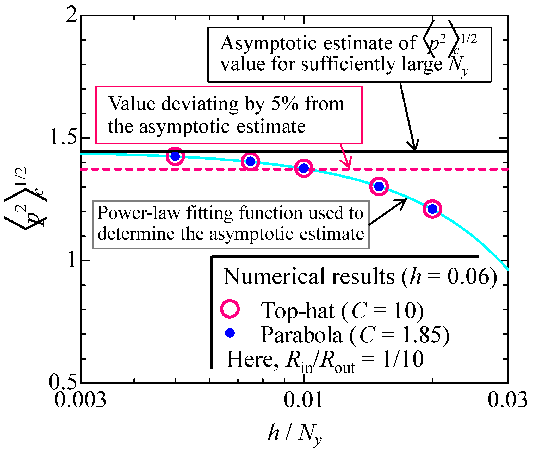
To evaluate the effect of wall-normal grid resolution on the first-order slip condition, calculations were performed for , for which the influence of wall slip is strongest and the number of grid layers in the wall-normal direction is smallest, using . The corresponding grid spacings were . The quantity evaluated was the converged spatial RMS of the levitation pressure, , which is the primary quantity of interest in the present study. As increased, increased monotonically and approached a finite asymptotic value as became sufficiently large, as shown in Figure A1. Compared with the asymptotic value obtained from a power-function fit to the dependence on , the value at , i.e., , adopted in the present study was approximately lower than the asymptotic value. Therefore, a wall-normal discretization uncertainty of approximately remains in the absolute value of the spatial RMS of the levitation pressure at . By contrast, the results for and were nearly identical, indicating that this grid dependence was almost independent of the prescribed blowing-velocity distribution.
The discretization error in the velocity gradient normal to the wall, which appears in the first-order slip condition, can also be evaluated from the thin-film approximation solution derived in the manuscript. In the present study, the in-plane velocity distribution under the first-order slip condition is given by . Because this velocity distribution is quadratic in y,
In general, when a second-order-accurate finite-difference approximation is used in the wall-normal direction, the discretization error in the wall-normal derivative of the in-plane velocity can formally be expressed as
Therefore, for the ideal lubrication-approximation solution given above, the leading second-order truncation error in the wall-normal derivative of the in-plane velocity vanishes.
Figure A1.
Wall-normal grid-resolution dependence of the converged pressure RMS under the first-order slip condition. Dependence of the converged pressure RMS, , on the wall-normal grid resolution, , at and , obtained by varying the number of wall-normal grid layers as , 4, 6, 8, and 12. Results are shown for the top-hat inlet velocity profile () and the parabolic inlet velocity profile (). The cyan curve represents the fit , , where , A, and q are fitting parameters. The fitted exponent was . The solid black line indicates the asymptotic estimate extrapolated to , whereas the magenta dashed line indicates a value below the asymptotic estimate. The result for , corresponding to and used in the present study, lies approximately on the deviation line.
Appendix A.2. Definition of the Levitation-Pressure RMS over the Three-Dimensional Computational Domain
The levitation-pressure RMS used in the present study is neither an area average restricted to a particular horizontal plane nor a temporal average; rather, it is a spatial RMS evaluated over the entire three-dimensional computational domain at each instant. Let denote the computational domain in the x–z plane, with . The three-dimensional spatial mean of the pressure is then defined as
and the RMS value of the spatial variation of the pressure is defined as
In the present computation, the spatial mean of the pressure is set to zero as the reference pressure so that , and therefore
Figure 10 shows the temporal evolution of this three-dimensional spatial RMS. The converged value used in Figure 11 and Figure 12 is defined as The pressure distributions at shown in Figure 9 are horizontal cross-sections used to visualize the pressure field, and the domain over which the RMS is evaluated is not restricted to this plane.
References
- Oiwa, N.; Masuda, M.; Hirayama, T.; Matsuoka, T.; Yabe, H. Deformation and flying height orbit of glass sheets on aerostatic porous bearing guides. Tribol. Int. 2012, 48, 2–7. [Google Scholar] [CrossRef] [Scilit]
- Li, G.X.; Tao, W.Q.; Li, Z.Y.; Yu, B. Direct numerical simulation of rarefied turbulent microchannel flow. Microfluid. Nanofluid. 2006, 2, 106–116. [Google Scholar] [CrossRef] [Scilit]
- Hadjiconstantinou, N.G. Molecular mechanics of liquid and gas slip flow. Annu. Rev. Fluid Mech. 2024, 56, 435–461. [Google Scholar] [CrossRef] [Scilit]
- Cheng, C.; Chen, J.; Zhao, M.; Liu, Z.X.; Xu, J.; Li, G.; Hou, Y.; Zhao, W. Micro-vibration control of an aerostatic bearing with micro cylindrical array. Phys. Fluids 2025, 37, 015217. [Google Scholar] [CrossRef] [Scilit]
- Suzuki, H.; Oka, H.; Fujiwara, J.; Kouchi, T. Inverse-cubic scaling of normalized static-pressure spatial variations in low-Reynolds-number air-film flows over suction-type floating stages. Int. J. Heat Fluid Flow 2026, 117, 110008. [Google Scholar] [CrossRef] [Scilit]
- Kim, J.; Moin, P. Application of a fractional-step method to incompressible Navier–Stokes equations. J. Comput. Phys. 1985, 59, 308–323. [Google Scholar] [CrossRef] [Scilit]
- Orlandi, P.; Bernardini, M.; Pirozzoli, S. Poiseuille and Couette flows in the transitional and fully turbulent regime. J. Fluid Mech. 2015, 770, 424–441. [Google Scholar] [CrossRef] [Scilit]
- Pirozzoli, S. Searching for the log law in open channel flow. J. Fluid Mech. 2023, 971, A15. [Google Scholar] [CrossRef] [Scilit]
- Morinishi, Y.; Lund, T.S.; Vasilyev, O.V.; Moin, P. Fully conservative higher order finite difference schemes for incompressible flow. J. Comput. Phys. 1998, 143, 90–124. [Google Scholar] [CrossRef] [Scilit]
- Suzuki, H.; Hattori, S.; Mochizuki, S. Numerical investigation using an exact solution of the effects of non-solenoidality of the viscous terms on the incompressible flow. J. Fluid Sci. Technol. 2017, 12, JFST0001. [Google Scholar] [CrossRef] [Scilit]
- Morinishi, Y.; Vasilyev, O.V. Vector level identity for dynamic subgrid scale modeling in large eddy simulation. Phys. Fluids 2002, 14, 3616–3623. [Google Scholar] [CrossRef] [Scilit]
- Oka, H.; Suzuki, H.; Fujiwara, J.; Kouchi, T. Time-scale identification and stretched-exponential modeling of flow-energy transients in a suction-type air bearing under gap-height steps. Int. J. Heat Fluid Flow 2026, 119, 110308. [Google Scholar] [CrossRef] [Scilit]
- Sone, Y.; Onishi, Y. Kinetic theory of evaporation and condensation—Hydrodynamic equation and slip boundary condition—. J. Phys. Soc. Jpn. 1978, 44, 1981–1994. [Google Scholar] [CrossRef] [Scilit]
- Ohwada, T.; Sone, Y.; Aoki, K. Numerical analysis of the Poiseuille and thermal transpiration flows between two parallel plates on the basis of the Boltzmann equation for hard-sphere molecules. Phys. Fluids A 1989, 1, 2042–2049. [Google Scholar] [CrossRef] [Scilit]
- Gibelli, L. Velocity slip coefficients based on the hard-sphere Boltzmann equation. Phys. Fluids 2012, 24, 022001. [Google Scholar] [CrossRef] [Scilit]
- Min, T.; Kim, J. Effects of hydrophobic surface on skin-friction drag. Phys. Fluids 2004, 16, L55–L58. [Google Scholar] [CrossRef] [Scilit]
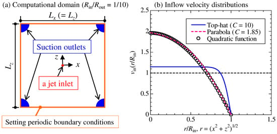
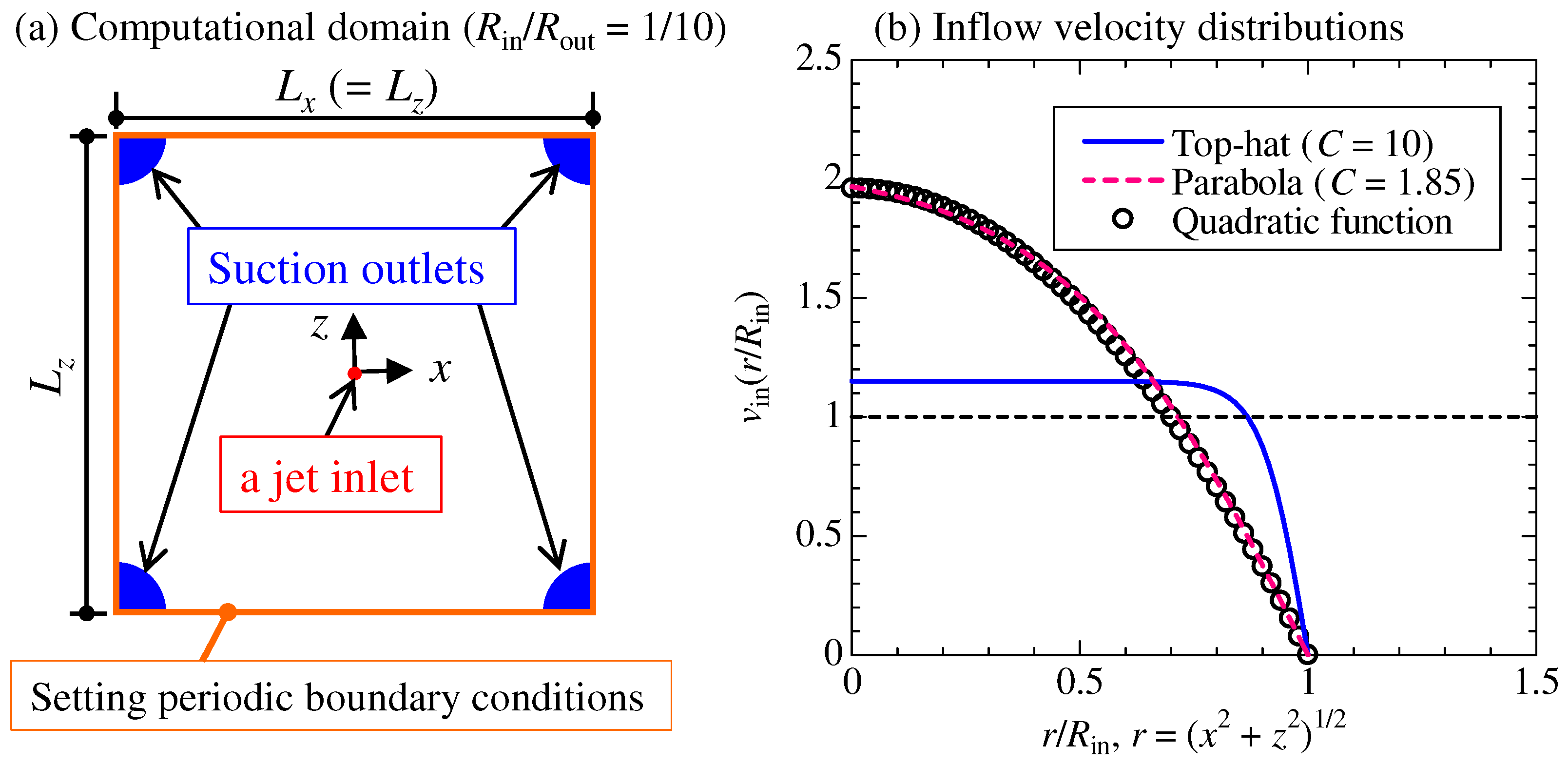
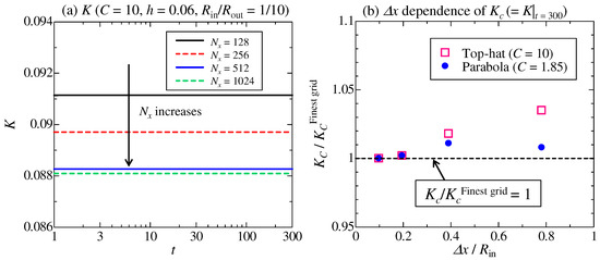
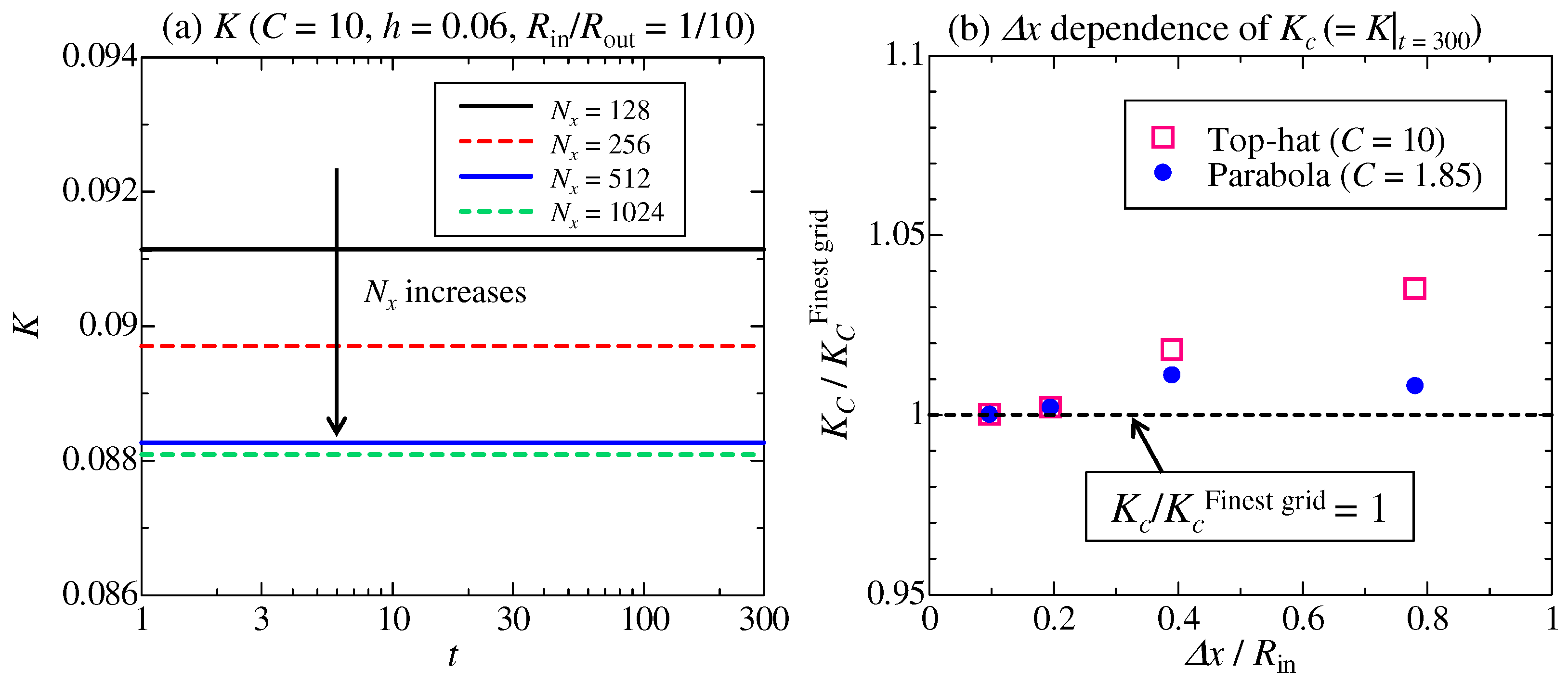
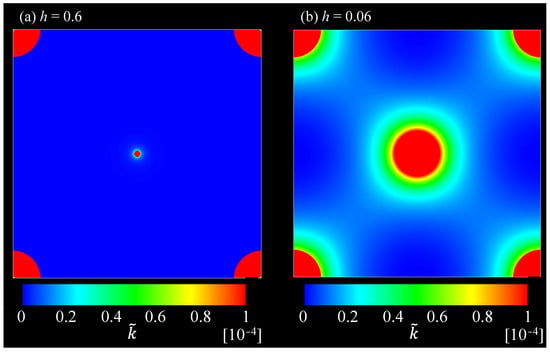
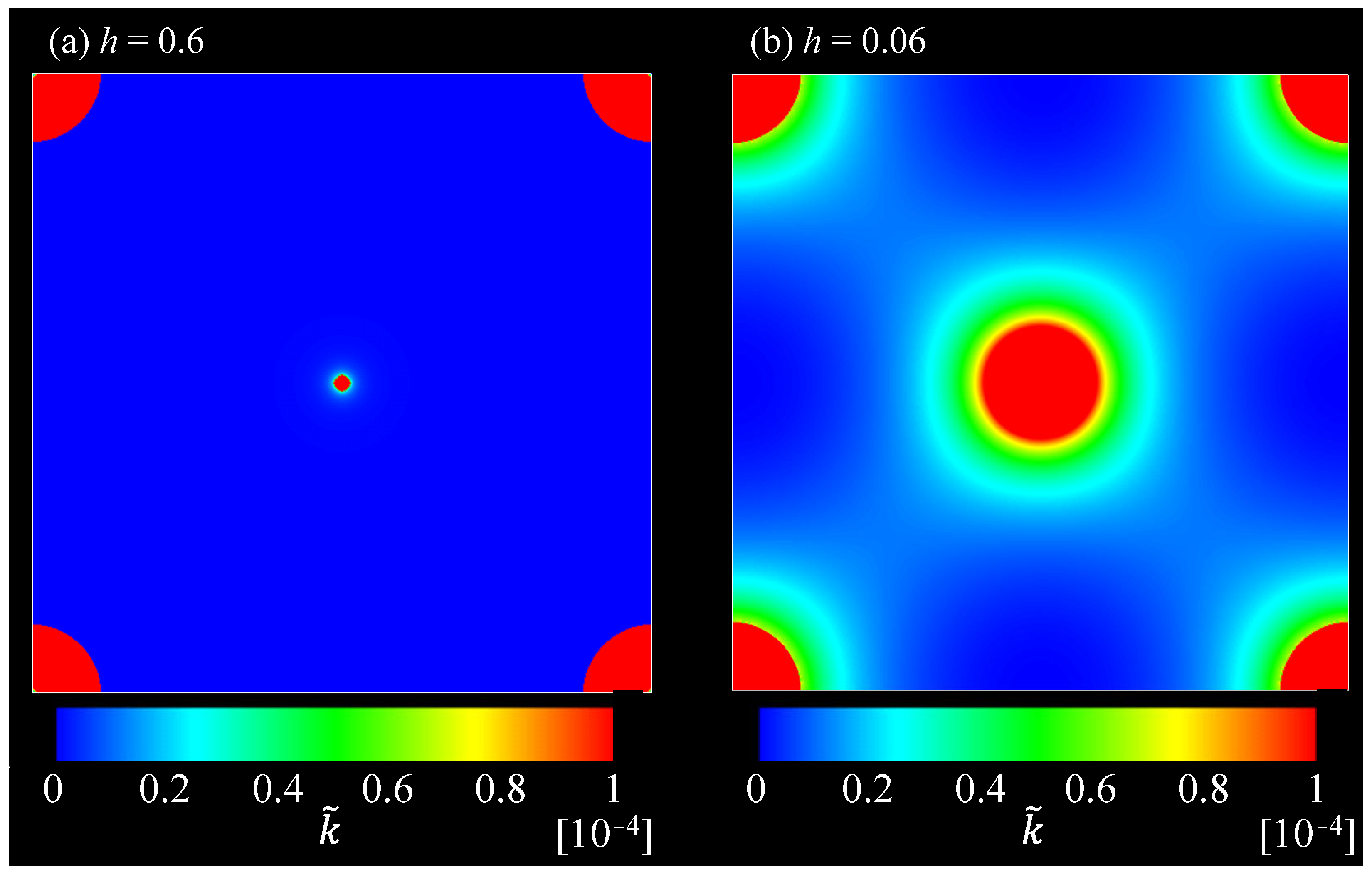
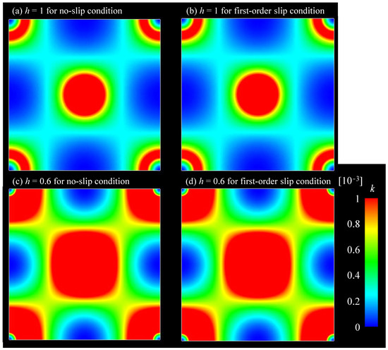
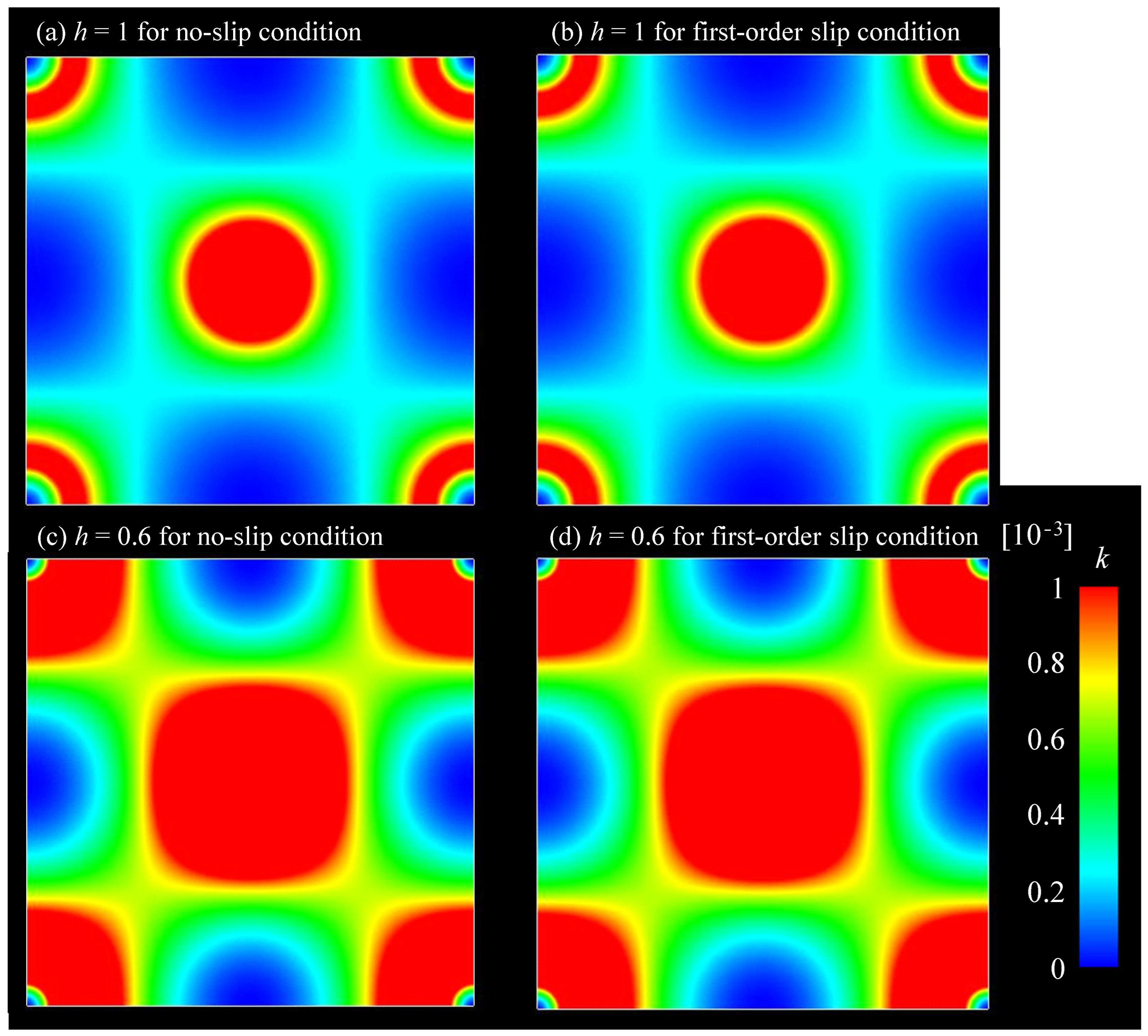
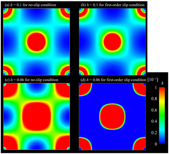
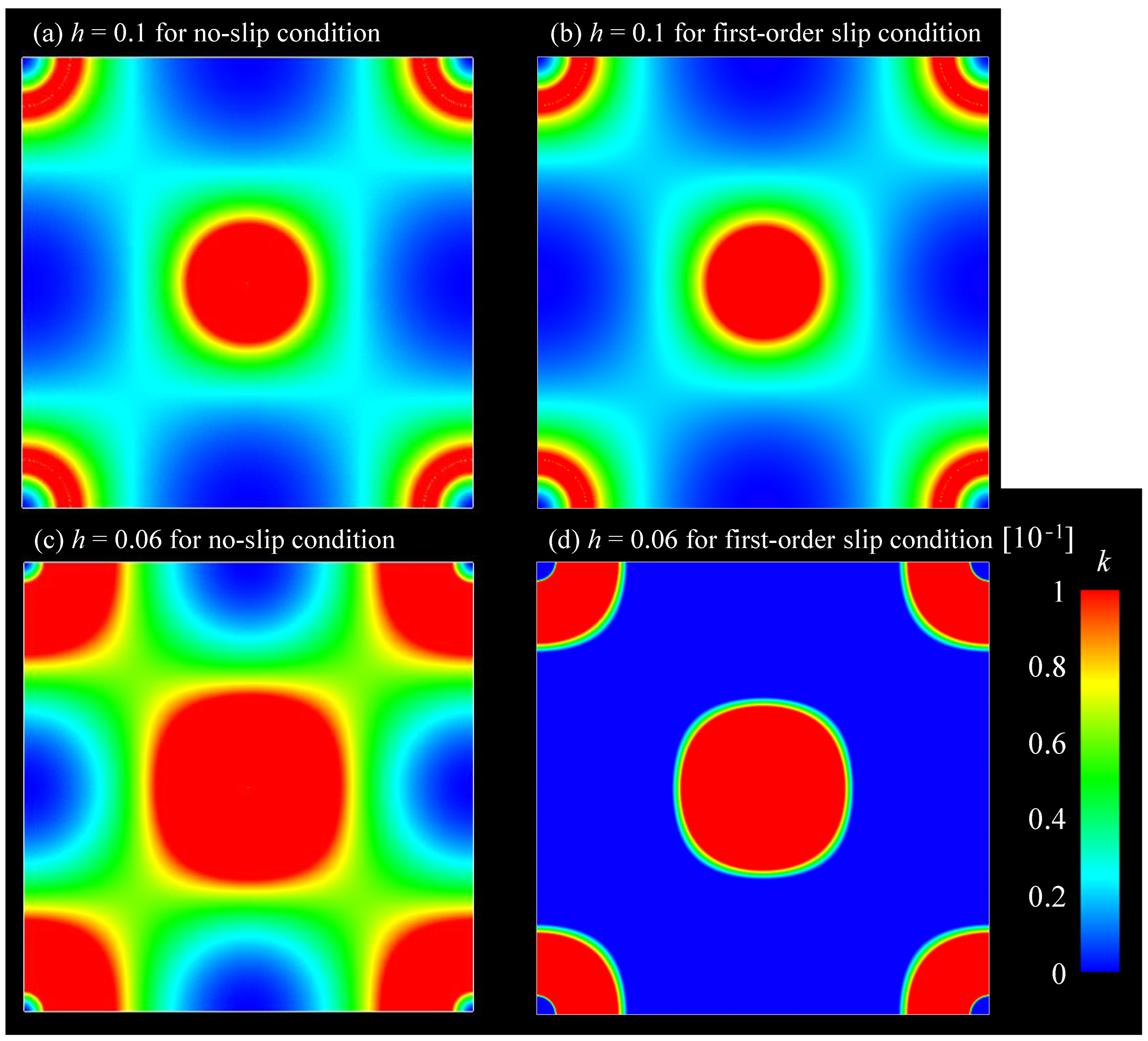
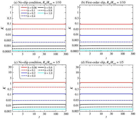
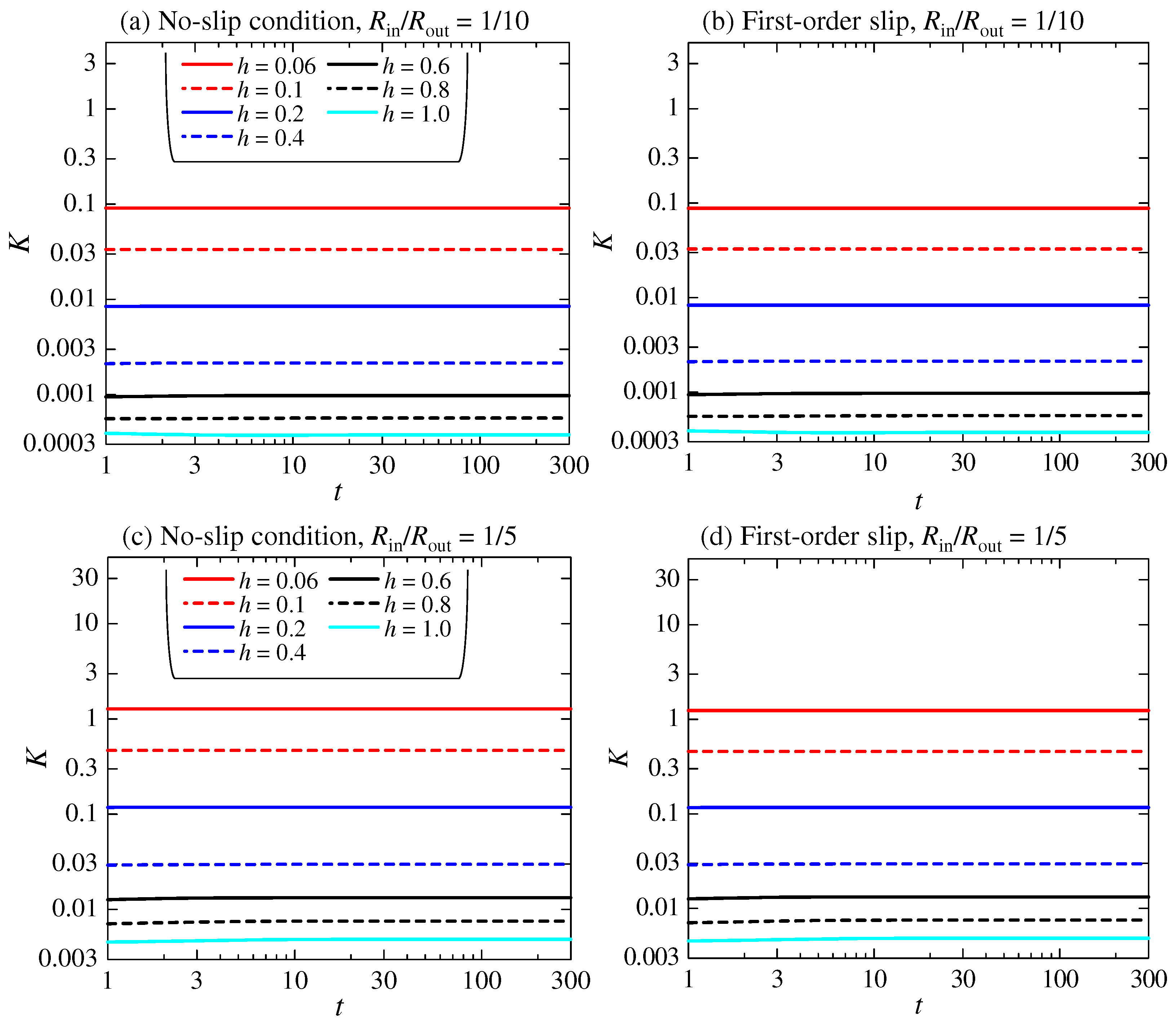
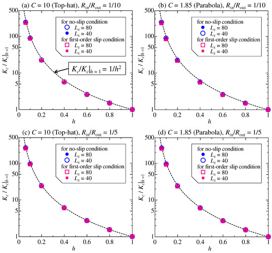
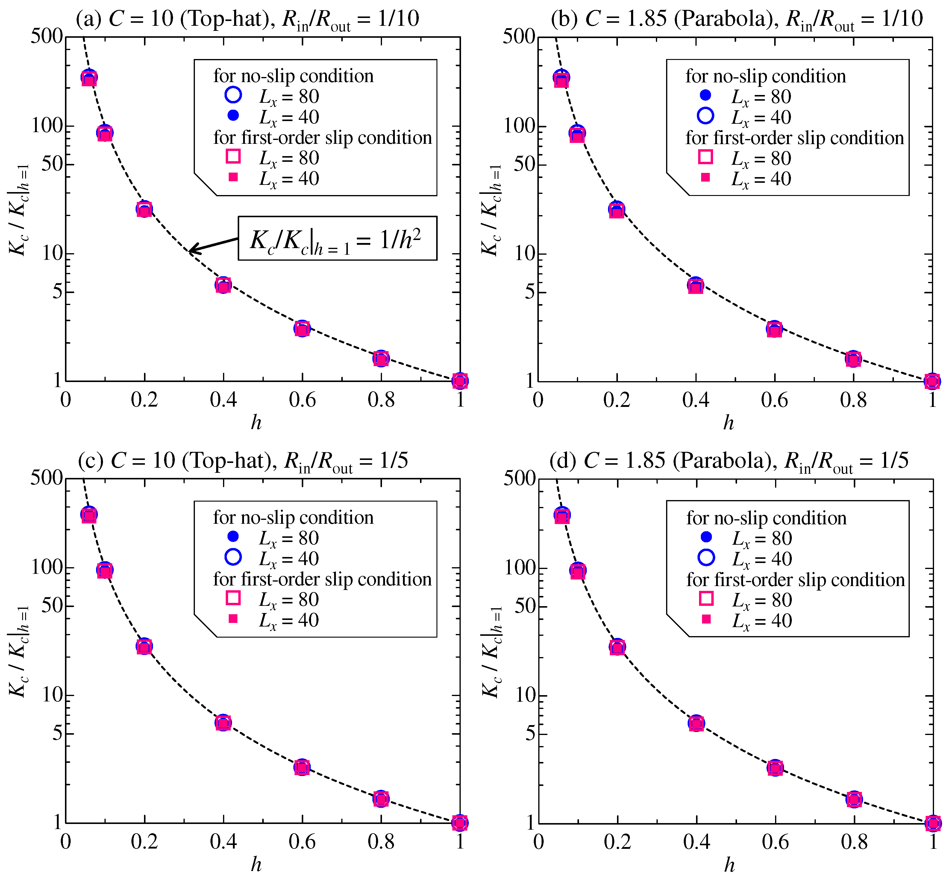
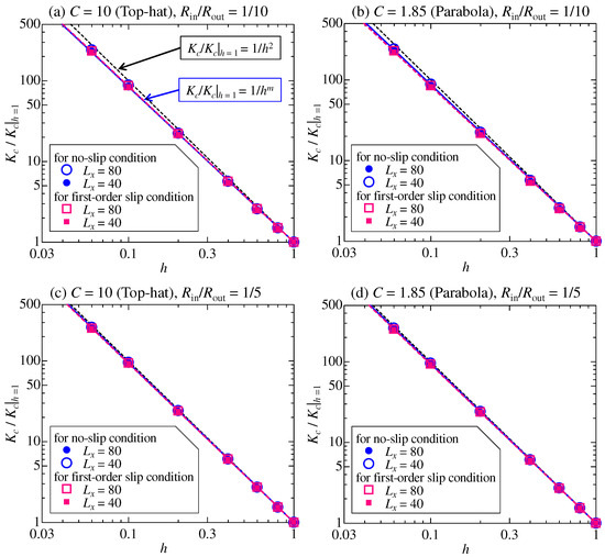
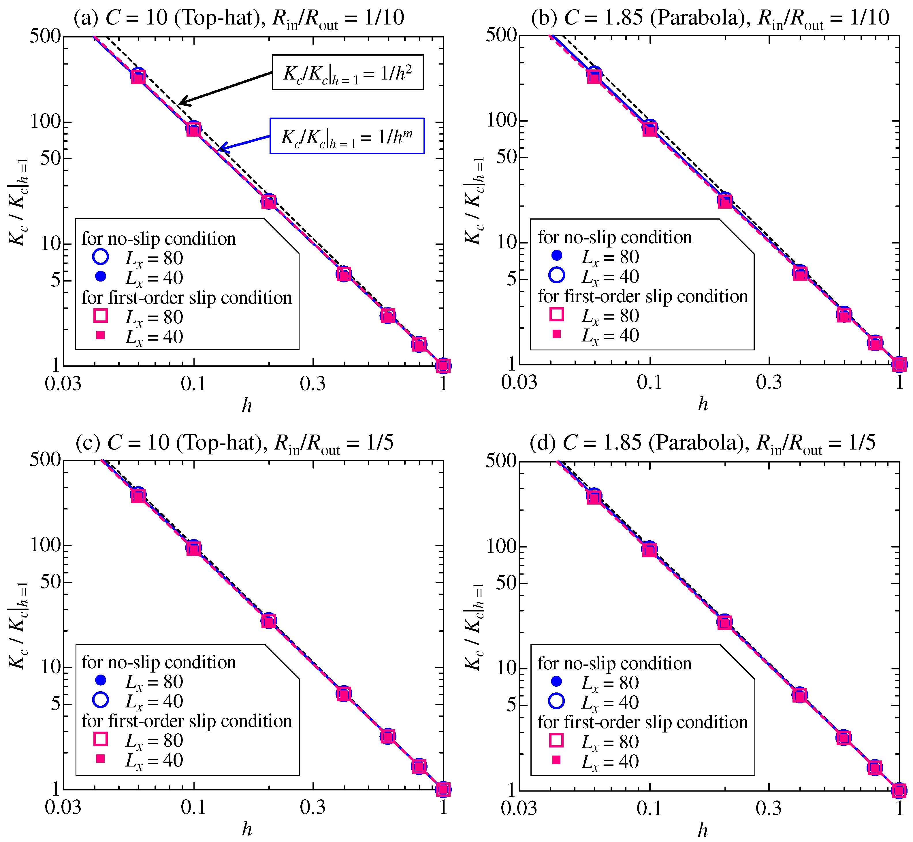
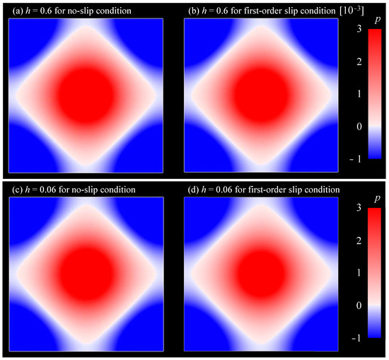
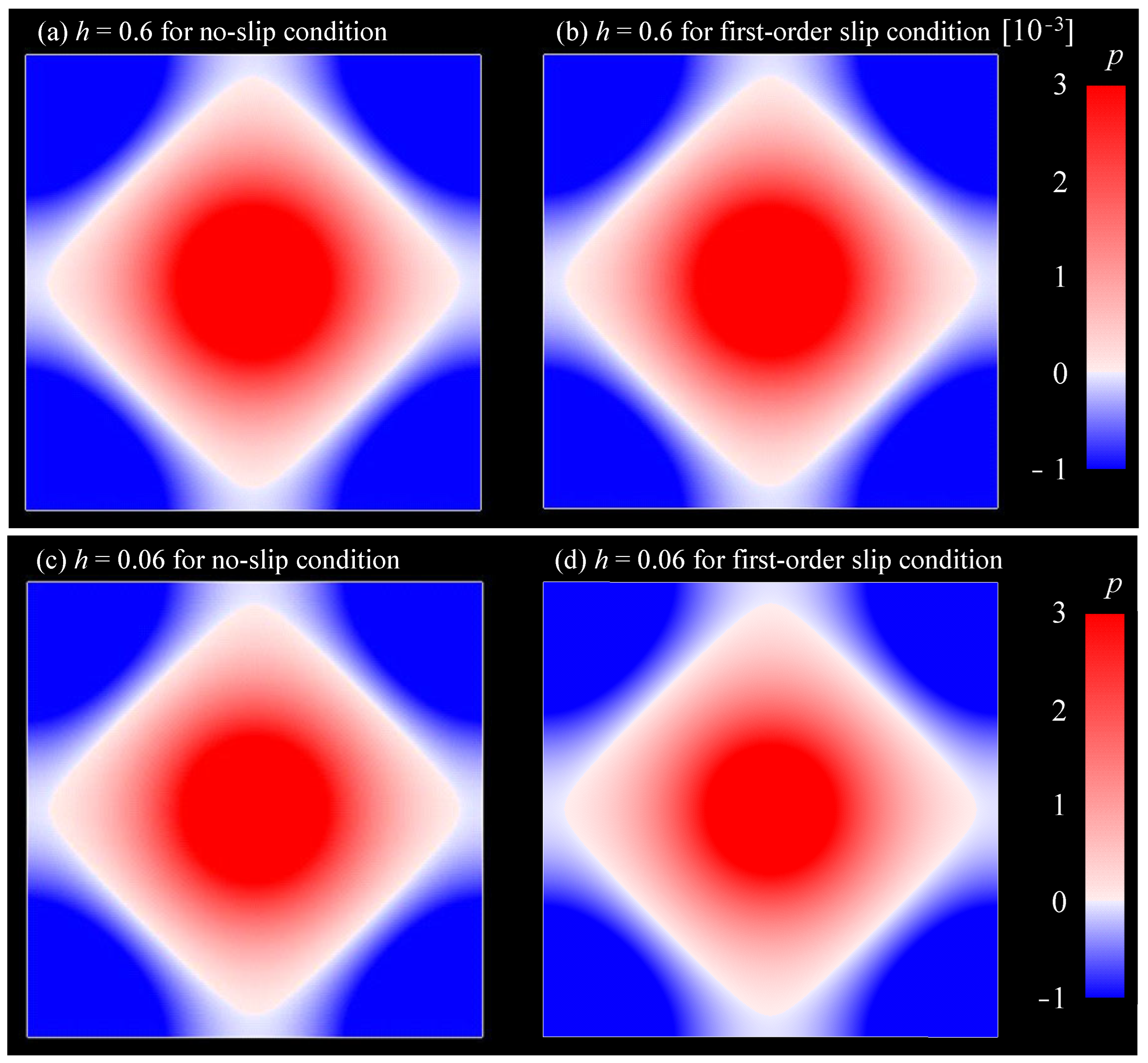
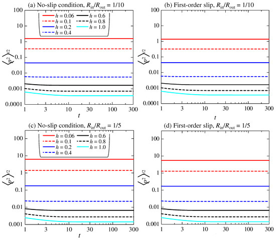
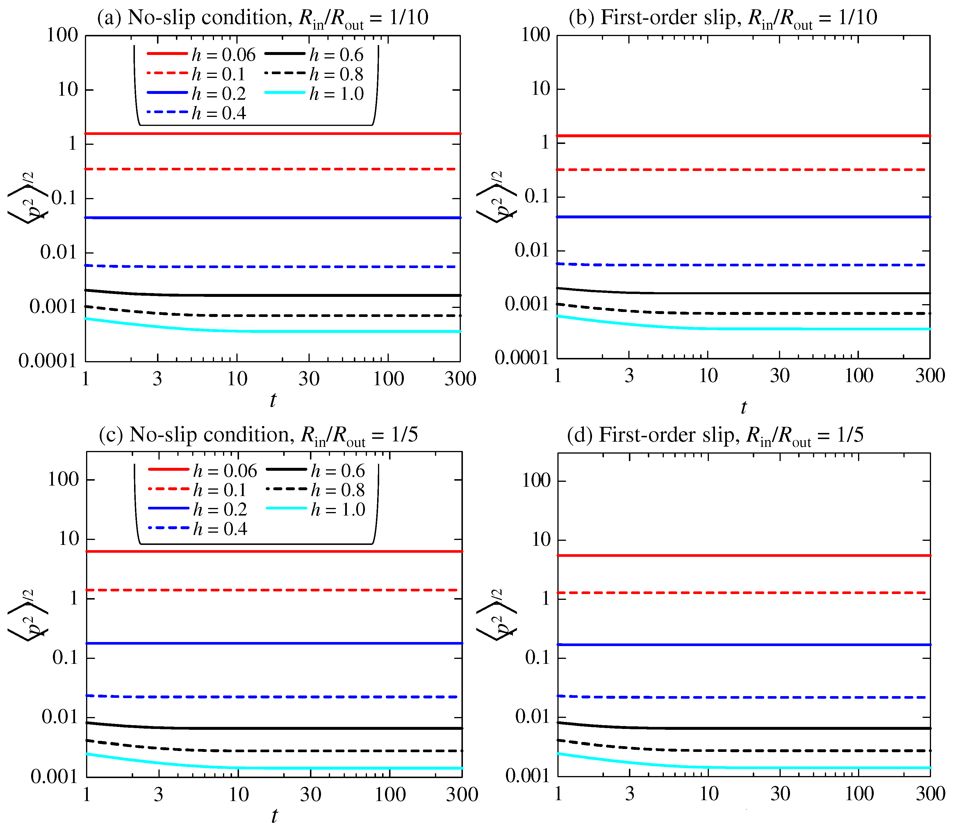
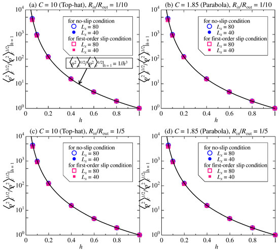
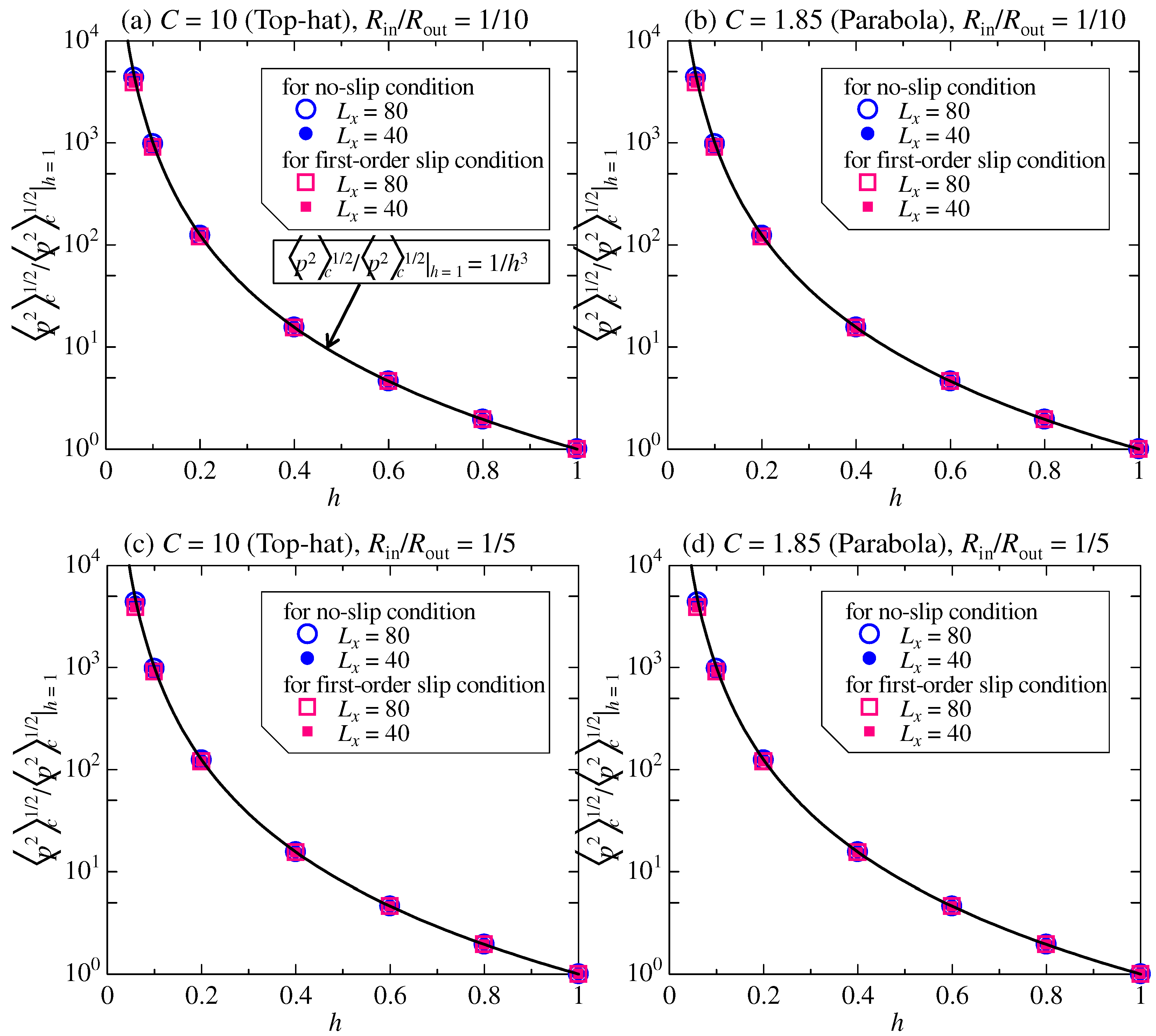
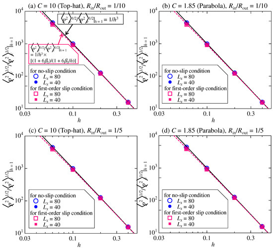
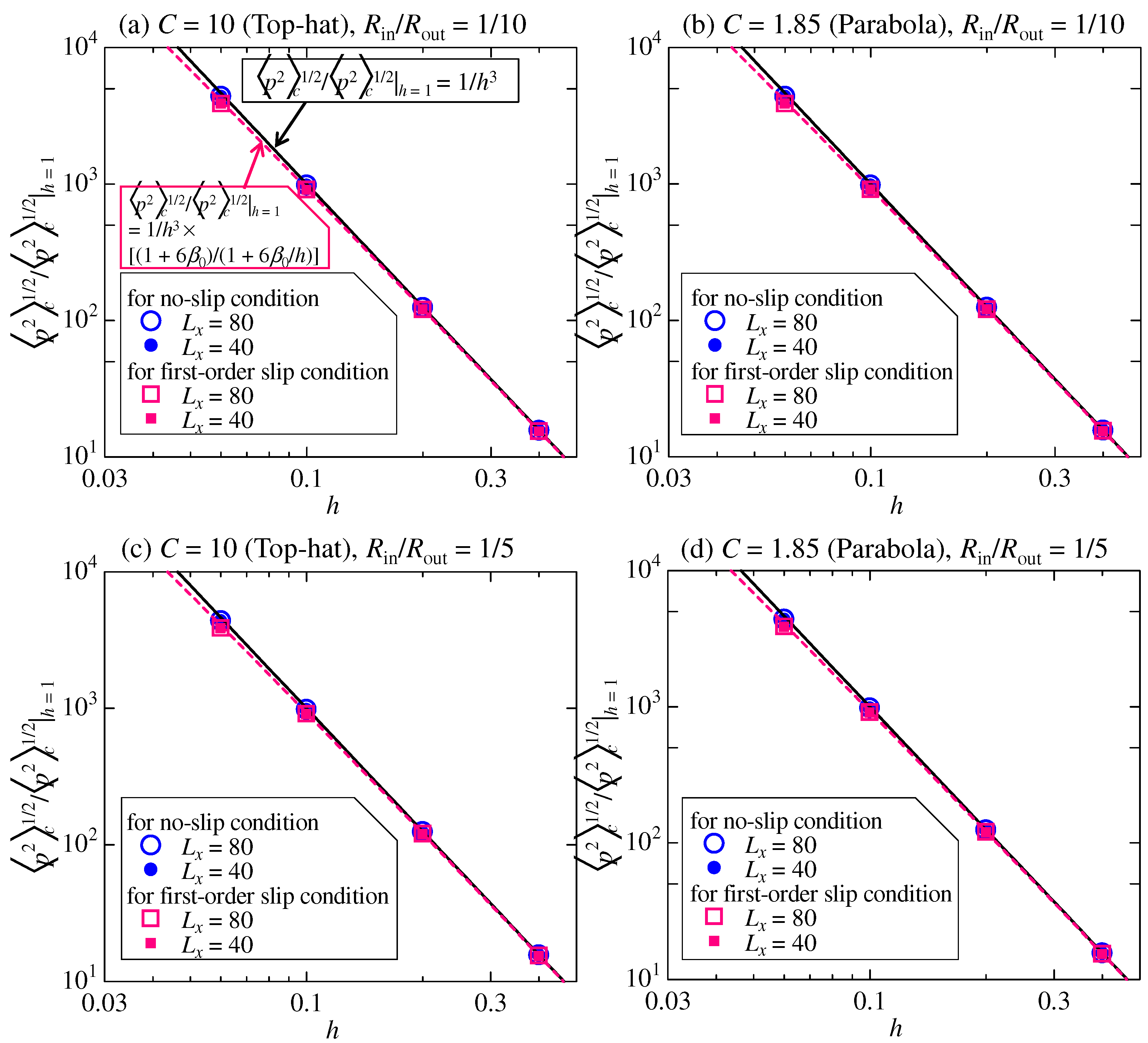
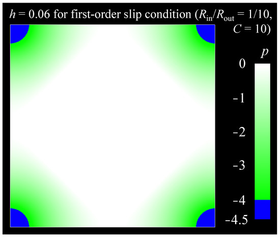
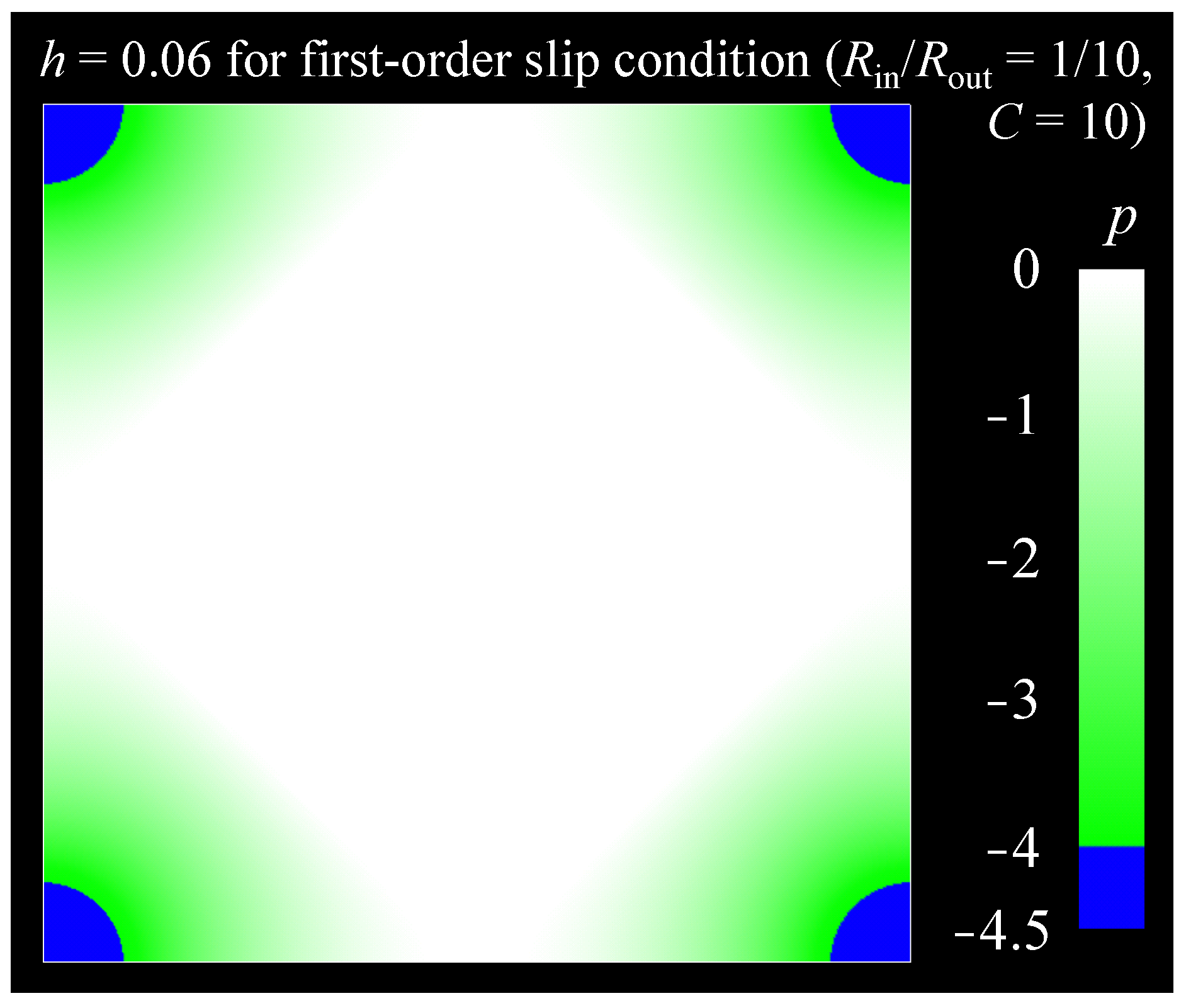
Disclaimer/Publisher’s Note: The statements, opinions and data contained in all publications are solely those of the individual author(s) and contributor(s) and not of MDPI and/or the editor(s). MDPI and/or the editor(s) disclaim responsibility for any injury to people or property resulting from any ideas, methods, instructions or products referred to in the content. |
© 2026 by the authors. Licensee MDPI, Basel, Switzerland. This article is an open access article distributed under the terms and conditions of the Creative Commons Attribution (CC BY) license.