


Abstract
Accurate identification of multiphase flow patterns in vertical pipelines is critical for operational safety and efficiency in the oil and gas industry. Yet, conventional methods struggle with subjectivity and transitional regimes. This study develops and integrates three neural network architectures: a convolutional neural network (CNN) for spatial features, a transformer neural network (TNN) for long-range dependencies, and a physics-encoding network (PEN) for embedding physical constraints. These are combined into a hybrid framework trained on an experimental dataset of 2131 images from a wire mesh sensor, annotated using a semi-automated pipeline. Results show the hybrid model achieved 95.91% test accuracy with a macro F1-score of 0.96, the highest of the four models evaluated, with its main advantage in transitional regimes. A multi-seed ablation shows that the convolutional branch provides the dominant discriminative signal, while the transformer and physics-inspired branches added complementary improvements that are consistent across runs. This hybridisation mitigates individual model weaknesses, with the physics-inspired branch acting as a spatial regulariser that improves interpretability, providing a robust and objective tool for reliable pipeline monitoring.
1. Introduction
Gas–liquid flows sit at the heart of many industrial processes, especially oil and gas production, where hydrocarbons move through vertical pipelines under changing pressure and velocity [1]. Such flows organise themselves into distinct regimes. Bubbly flow disperses gas bubbles through a continuous liquid phase; slug flow alternates elongated gas pockets with liquid slugs; churn flow mixes the phases chaotically; and annular flow wraps a gas core in a liquid film [2,3]. Between these lie transitional states such as bubbly-to-slug or slug-to-churn flows, and they complicate the picture further because they mark unstable conditions set by superficial velocities, pipe geometry, and inclination [4].
Getting the regime right matters. It bears directly on heat transfer, pressure drop, and operational risks such as slug-induced vibration or liquid holdup [5,6]. Gravity reinforces the flow direction in vertical pipelines, so transitions arrive more abruptly than in horizontal systems, which raises the premium on accurate detection for sustaining throughput and avoiding inefficiency [7]. Doing this in the field is hard. Industrial flows change quickly, the pipelines are opaque, and direct visualisation is usually impossible. Lai et al. [8] make the point that slug flow in risers throws up strong transient fluctuations in pressure, velocity, and holdup that steady or quasi-steady mechanistic models cannot capture, which exposes the limits of the traditional approaches.
The core difficulty is recognising flow patterns precisely and in real time in settings where watching by eye is impractical. The traditional options, high-speed imaging with visual inspection or mechanistic models built on drift–flux theory, each fall short. Visual inspection is subjective and varies from one observer to the next, while mechanistic frameworks lean on empirical parameters that break down outside the conditions they were tuned for, such as vertical downward slug flow [7]. Neither classifies transitional regimes reliably because their overlapping features blur the distinctions and undermine automated monitoring [9].
In two-phase vertical pipe flow, the regime is characterised chiefly by void fraction, the fraction of the pipe cross section taken up by the gas phase, together with related quantities such as the edge pixel count, bubble count, interface length, and interfacial area concentration [10,11]. These describe the geometry and structure of the gas–liquid interface that tells one regime from another. Transitional regimes, though, do not sit at fixed threshold values of any single parameter. They emerge as several spatial and structural features shift together with the flow conditions, which is why parameter-based rules alone cannot separate them cleanly. Machine learning has the advantage here. Instead of learning on pre-set boundaries, it learns spatial representations straight from the image data, and those representations implicitly reflect the same physical quantities. In the present framework, the CNN picks up local features tied to void fraction distribution and gas–liquid interface geometry across the cross section, both linked directly to the edge content and interfacial area concentration [10]. The TNN reads spatial relationships over the whole cross section, capturing global phase distribution patterns that single-point measurements miss. The PEN enforces smoothness in the learned features, in keeping with the expectation that transitional regimes in the phase structure change gradually rather than abruptly. None of these branches introduces a new fundamental physical parameter. Instead, they learn data-driven representations that track established physical descriptors and carry across the regime boundaries where threshold-based methods fail.
Faced with these shortcomings, researchers have moved to machine learning. Table 1 reviews the key studies, and it shows a clear progression from classical ensemble methods to modern deep learning architectures. The early work applied support vector machines to probe-derived features and achieved accuracies near 80%, but only through labour-intensive feature engineering [12]. Deep learning widened what was possible. Convolutional neural networks (CNNs) paired with synchrosqueezing wavelet transforms of accelerometer-derived displacement signals have classified flow regimes well: Azam et al. [9] report accuracies of 83.55%, 92.76%, and 97.88% for AlexNet, VggNet, and ResNet, respectively. Transformer models, first built for sequential tasks, have since been adapted to vision problems, where they capture long-range dependencies effectively [13]. Physics-Informed Neural Networks (PINNs), which impose governing differential equations as hard constraints and take spatiotemporal coordinates as inputs, have shown promise in extrapolating fluid dynamics [14].
Each paradigm still has its weak points. CNNs often miss global interactions, transformers need large, labelled datasets, and PINNs depend on explicit governing equations and boundary conditions that image-based classification does not always provide. The decisive gap, as the literature in Table 1 makes clear, is that no existing framework brings these complementary approaches together in one unified architecture for multiphase flow classification.
To avoid the intrusion-related limitations of sensors such as wire mesh sensors and conductance probes, several non-intrusive approaches have been explored. One class of methods exploits Flow-Induced Vibration (FIV) signals captured by force or acceleration sensors mounted externally on the pipe wall. Wang et al. [15] developed a 1D convolutional neural network trained on FIV acceleration signals from a 90-degree elbow section, achieving an average classification accuracy of 89.9% across multiple flow regimes in an industrially representative setup. Similarly, Qiao et al. [16] developed a multi-input parallel convolutional neural network (CWT-Mul-LeNet) trained on continuous wavelet transform representations of vibration signals from the vertical section of subsea pipelines, achieving a classification accuracy of 99.69% across four flow patterns without requiring any flow intrusion. A second class of non-intrusive approaches exploits differential pressure fluctuations measured via external wall taps. Shaban and Tavoularis [17] applied the elastic maps algorithm to the probability density function of differential pressure signals in vertical upward air–water pipe flow, demonstrating that the method is robust to variations in pipe diameter (13.9–49.2 mm) and absolute pressure (100–240 kPa), making it amenable to practical calibration. These non-intrusive methods bring clear industrial advantages, but they respond mainly to bulk hydrodynamic signatures and frequency-domain features, and they usually need dedicated signal-processing pipelines. Image-based approaches using wire mesh sensors sit at the other end. They are intrusive, yet they deliver rich spatial information about phase distribution and interfacial structure, which allows direct visual characterisation of seven distinct regimes, transitional states included, that signal-based methods alone resolve poorly [10].
This study sets out to close that gap with a hybrid neural network that integrates CNNs, transformers, and PENs. Building and rigorously validating a high-performance algorithm of this kind depends on high-fidelity ground-truth data. The data were therefore drawn from a wire mesh sensor (WMS), an intrusive technique that records detailed cross-sectional phase distribution and is well suited to training and benchmarking complex neural network architectures. The WMS is a laboratory tool, but the core contribution is a transferable methodology: a model that can pick out subtle visual features while respecting physical constraints. The longer-term aim is to run this trained architecture, or a version fine-tuned from it, in the field with non-intrusive sensors such as high-speed cameras or pressure transducers, where it can deliver the same intelligent, real-time flow pattern identification without disturbing the flow.
The model classifies seven regimes from an experimental dataset of pipeline imagery: bubbly, bubbly–slug transition, slug, slug–churn transition, churn, churn–annular transition, and annular. Seven regimes were chosen rather than the three or four classes common in thermo-fluid studies because transitional states carry real operational weight in pipeline monitoring. Grouping flows into bubbly, slug, churn, and annular is enough for steady-state heat transfer and pressure-drop correlations, but it cannot tell a fully developed regime from one that is actively changing. That distinction has practical consequences in vertical pipelines. The slug–churn transition sets in as the liquid bridges between Taylor bubbles start to break down, and it produces pressure fluctuations unlike those of stable slug or churn flow [6]. The churn–annular transition, in turn, forms a partial liquid film at the pipe wall while turbulent mixing continues at the core, a condition that neither adjacent stable class captures [2]. Getting these transitional states wrong can lead to the wrong control decision at exactly the moment when instabilities such as pressure surges or liquid holdup are most likely [5,6]. Detecting the onset of a transition early therefore has operational value that a coarser classification cannot offer. The 24 × 24 wire mesh sensor used here captures cross-sectional phase distribution images detailed enough to separate all seven regimes visually, and the dataset, drawn from 52 test runs, supplies adequate samples per class (Table 2). This seven-class taxonomy follows prior image-based studies in vertical pipelines [18], which supports both its feasibility and its scientific relevance.
The methodology begins by annotating a 700-image subset with YOLOv8, and this subset then guides the automated labelling of the full dataset of 2131 images through a TinyLlama-based pipeline. The dataset is split into training, validation, and test subsets, with training carried out end to end in Google Colab.
The principal contributions of this study are as follows. First, a hybrid neural network integrating CNN, transformer, and physics-encoding network branches is proposed and validated for multiphase flow pattern classification in vertical pipelines, addressing the limitations of each individual architecture when applied in isolation. Second, the PEN branch introduces gradient-based spatial regularisation as a physics-inspired training objective, applying a physically motivated smoothness prior to image-based classification without requiring explicit governing equations or boundary conditions. As detailed in Section 2.5, this is a physics-inspired regulariser rather than a physics-informed neural network in the conventional sense. Third, a semi-automated annotation pipeline that combines YOLOv8 object detection with TinyLlama natural-language labelling and physics rule-based correction is developed to generate first-pass labels that are then verified and corrected by a domain expert, reducing the manual effort of large-scale WMS image labelling relative to fully manual annotation. Fourth, the model classifies seven flow regimes, including three transitional patterns (bubbly–slug, slug–churn, and churn–annular), providing finer-grained classification than most comparable works. Fifth, model decisions are interpreted using Grad-CAM heatmaps, transformer attention maps, and physics activation patterns, supporting transparent and physically grounded classification.
The remainder of this paper is organised as follows. Section 2 details dataset preparation and the model architecture. Section 3 presents the experimental results and discussion. Section 4 concludes with the study’s contributions and outlines directions for future research.
Table 1.
Comparative summary of machine learning applications for multiphase flow pattern identification.
Table 2.
Dataset distribution.
2. Materials and Methods
2.1. Dataset Preparation
This study employed experimental images of vertical pipeline flows obtained from 52 test runs using a 24 × 24 wire mesh sensor (WMS), which captured sequential cross-sectional views of air–silicone oil mixtures [10]. The 52 test runs were systematically designed to span a comprehensive range of superficial gas and liquid velocities, ensuring the capture of all stable flow regimes (bubbly, slug, churn, annular) and the critical transitional states between them. From these runs, a total of 2131 representative images were extracted and classified into seven distinct patterns. The distribution of images across these flow regimes is detailed in Table 2. The schematic flow process, wire mesh sensor, and experimental rig (Figures S1 and S2) used to collect the data for this study are shown in the Supplementary Materials.
Annotation began with a curated subset of 700 images, evenly distributed across the seven classes (100 per class). These images were manually processed using Roboflow software (version 1.3.13) to produce YOLOv8-compatible annotations. Each annotation consisted of bounding boxes around relevant regions, paired with class labels to enable supervised training. This manually labelled subset provided the foundation for training an automated labelling pipeline, which was then applied to the entire dataset of 2131 images.
The 2131 images were divided into training (1493), validation (320), and test (318) subsets, with all seven flow classes represented in each subset (Table 2). Because the dataset consists of frames extracted from wire mesh sensor acquisitions, in which successive frames can appear visually similar, a leakage audit was performed to confirm that the test set did not contain near duplicates of the training images. Each image was encoded with a 64-bit perceptual difference hash, and the Hamming distance between every test and validation image and its closest training image was computed. No exact duplicates were found, and no test or validation image fell within a Hamming distance of eight bits of any training image, the range associated with near-identical frames. The smallest cross-subset distance was nine bits for the test set and ten bits for the validation set, with a median of seventeen bits, indicating that even temporally adjacent frames differ substantially because the wire mesh sensor records a rapidly evolving cross-sectional phase distribution. The reported performance therefore reflects generalisation to genuinely unseen frames rather than the memorisation of duplicated images. To further confirm that these results are not an artefact of a particular partition, a repeated cross-validation analysis is reported in Section 3.7.
2.2. Auto-Labelling Pipeline
The auto-labelling pipeline extended annotations from the manually labelled 700-image subset to the full 2131-image dataset by integrating a fine-tuned large language model with a physics-encoded rule-based correction system. It is important to emphasise that TinyLlama was not used as a standalone classifier; its probabilistic outputs served as an initial proposal that was subsequently corrected and overridden where necessary by a deterministic rule-based module whose thresholds were derived entirely from the empirical feature distributions of the 700 manually annotated images (Table 3). This design ensured that every automatically proposed label passed through physics-grounded constraints before being presented to a domain expert, who reviewed and corrected the proposals to produce the final labels. The language model’s role was therefore limited to interpreting structured numerical feature descriptions; it did not have access to raw images and could not fabricate visual content. All classification decisions were ultimately governed by the physically motivated thresholds in Table 3, which link measurable image features (colour ratios, edge density, edge pixel count, gradient magnitude) to established flow regime indicators such as gas holdup and the interfacial area [10].
Table 3.
Rule-based thresholds for flow pattern identification using physical features.
Each image was represented by an eight-dimensional feature vector (Equations (1)–(8)) quantifying structural and intensity-based attributes, a technique demonstrated to be effective using texture descriptors such as Local Binary Patterns (LBPs) [25]:
- Edge Ratio ():
- ii.
- Mean Intensity ():
- iii.
- Gradient Magnitude Mean ():
- iv.
- Red Hue Ratio (): the proportion of pixels whose HSV hue angle falls within the red range (hue channels 0–5 and 150–180 out of 180), computed from the normalised hue histogram of the image:
- v.
- Edge Pixel Count ():
- vi.
- Edge–Bubble Ratio ():
- vii.
- Gradient–Edge Product
These metrics provided discriminative cues; for example, low with high typically indicated bubbly flow with sparse blue bubbles, while high and low corresponded to annular flow dominated by blue liquid films.
The language model component employed TinyLlama-1.1B-Chat-v1.0, selected for its efficiency in converting numerical features into text while retaining reasoning capacity at modest computational cost [26]. The choice of a language model for this stage, rather than a conventional classifier such as a support vector machine or random forest, was motivated by the labelling workflow rather than by classification accuracy. The language model produces a short natural-language justification alongside each proposed label, which made the subsequent expert review faster and more transparent. The structured natural-language prompt provides a flexible interface for combining the engineered features with their physical interpretation. A conventional feature-based classifier could perform the same numeric feature-to-label mapping; the language model was not selected because it is more accurate, and indeed the accuracy of this automated stage is modest, as quantified in the label quality assessment. The reliability of the final labels rests on the deterministic physics-based rules and the expert verification step, with the language model serving only to generate an interpretable first-pass proposal. This is consistent with the semi-automatic design of the pipeline, in which every label was ultimately verified by a domain expert. The 700 annotated images served as training data. For each sample, extracted features were embedded into a structured prompt:
The flow image shows edge complexity of [], mean intensity of [], gradient magnitude of [], red hue ratio of [], blue hue ratio of [], edge pixel count of [], edge–bubble ratio of [], and gradient–edge product of []. Based on these, classify the multiphase flow pattern as one of bubbly, transition_bubbly–slug, slug, transition_slug–churn, churn, transition_churn–annular, and annular.
This format elicited both labels and reasoning chains, ensuring interpretability. Fine-tuning was performed using low-rank adaptation (LoRA), with and , applied to the [“q_proj”, “v_proj”] modules, with four-bit quantisation (BitsAndBytes, NF4, double quantisation) to reduce memory costs [27]. Training employed the AdamW8bit optimiser, with a learning rate of , batch size of four, and 30 epochs, producing probabilistic outputs for each class.
To ensure physical plausibility, outputs were corrected using a rule-based module informed by empirical flow physics and derived directly from the feature distributions of the manually labelled subset (Table 3). The thresholds were established by analysing the extracted image features (e.g., colour ratios, edge density, edge pixel count, and gradient magnitude) across the annotated dataset and then codified into explicit rules within the correction function. In this formulation, thresholds for colour ratios were aligned with gas holdup, while edge-derived metrics were linked to the interfacial area, two key indicators in flow regime classification [11]. These empirically grounded constraints refined the language model’s predictions, particularly in transitional zones, where visual ambiguity is highest. The credibility of the pipeline labels rests primarily on the rule-based correction module, which acts as a hard filter; any label inconsistent with the physically motivated thresholds in Table 3 is overridden regardless of the language model’s output, ensuring that all assigned labels comply with established flow regime physics. Within the automated stage, the rule-based module applies physics-grounded thresholds (Table 3) that override language model outputs inconsistent with them. As quantified in the label quality assessment below, this automated stage alone does not achieve expert-level accuracy, particularly for the transitional regimes, so its outputs were treated as proposals; the final labels were established by expert review and correction rather than by the automated rules alone. The resulting pipeline combined interpretability, computational efficiency, and physics-aware correction, enabling scalable annotation of the full dataset while maintaining fidelity to established multiphase flow regime definitions.
To quantify the reliability of the automated stage of the pipeline, its labels were compared against an independent expert assessment. A domain expert who was not involved in developing the pipeline manually labelled a random sample of 140 images, 20 per class, using only the images and without reference to any existing label. The automated stage, comprising the fine-tuned TinyLlama classifier followed by the physics rule-based correction, was then run on the same images, and its labels were compared with the expert labels. The automated stage agreed with the expert on 47.1% of the images, with a Cohen’s kappa of 0.38. The agreement was strongly regime-dependent: the automated stage reproduced the expert labels well for the visually distinct regimes, achieving an F1-score of 0.92 for annular, 0.81 for the churn–annular transition, and 0.60 for churn, but it performed poorly on the ambiguous transitional regimes, over-assigning the bubbly class and failing to identify the bubbly–slug and slug–churn transitions. The full confusion matrix and per-class agreement scores are provided in the Supplementary Materials (Figure S3 and Table S1). This limited and regime-dependent accuracy is the reason the pipeline is described as semi-automatic rather than automatic. The automated labels were treated as an initial proposal; every proposed label across the full dataset was subsequently reviewed by a domain expert and corrected wherever it disagreed with the expert’s visual assessment so that the final training labels are expert-verified. The automated stage therefore reduced manual effort by supplying a first-pass proposal and a structured feature summary for each image, while the accuracy of the final labels is that of the human expert rather than that of the automated stage.
The discriminative image features learned by each model branch are examined in Section 3.3 through Grad-CAM explainability visualisations, providing direct insight into the spatial regions and structural characteristics that drive classification decisions for each of the seven flow regimes.
2.3. The CNN Architecture
A CNN is implemented using TensorFlow to extract hierarchical features through successive convolutional operations (Figure 1), following established design principles for spatial feature extraction [28]. The model consists of five convolutional blocks, each comprising a 3 × 3 convolution with LeakyReLU activation (negative slope 0.1), batch normalisation [29], and 2 × 2 max-pooling. Filter sizes increment from 32 to 512 across the blocks to capture spatial features hierarchically. The flattened output passes through a 512-unit dense layer with ReLU activation and 50% dropout [30] before branching into two heads: a four-neuron sigmoid-activated layer for bounding box regression and a seven-neuron softmax layer for class prediction. The convolution operation is given by Equation (9):
where is the input feature map, the kernel weights, the bias, and the kernel size.
Figure 1.
CNN architecture for spatial feature extraction in flow pattern classification.
2.4. The TNN Architecture
The TNN architecture combines initial convolutional processing with transformer-based feature transformation, as shown in Figure 2. While traditionally used for sequential data, the self-attention mechanism in transformers is equally adept at modelling long-range spatial dependencies within a single image. This is crucial for multiphase flow, where the state of one region (e.g., a gas slug) can be contextually dependent on a distant region (e.g., the liquid film). Three convolutional blocks (32, 64, 128 filters, 3 × 3 kernels, ReLU activation) perform preliminary feature extraction, each followed by 2 × 2 max-pooling. The resulting features are partitioned into non-overlapping 8 × 8 patches, linearly projected into a 192-dimensional embedding space. Positional information is incorporated via learned embeddings, supplemented with a trainable classification token. The transformer component comprises six identical encoder layers, each implementing multi-head self-attention (six heads) with residual connections and layer normalisation [31,32], followed by pointwise feed-forward networks (384-unit hidden dimension, GELU activation) [33]. Regularisation includes dropout at all transformer layers. The attention mechanism computes as shown in Equation (10):
where are query, key, and value matrices and the key dimension.
Figure 2.
TNN architecture for capturing long-range dependencies in flow patterns.
2.5. The PEN Architecture
This study develops a PEN for multiphase flow pattern classification, incorporating spatial smoothness constraints through a gradient-based regularisation term (Figure 3) [34]. Unlike classical PINNs, which embed PDE residuals as hard constraints on field variables [34], the PEN encodes physical priors through a spatial gradient penalty on learned feature maps, a formulation appropriate for image-based classification tasks where flow field variables are not directly available. This approach is more accurately characterised as physics-inspired regularisation than PDE-constrained learning [35].
Figure 3.
PEN architecture with gradient-based regularisation for flow pattern classification.
The physics-encoding component penalises abrupt spatial variations in the learned feature maps, inspired by the gradient-enhanced PINN (gPINN) framework proposed by Yu et al. [36]. The physics loss function computes squared first-order finite differences between adjacent pixels in both vertical and horizontal directions, as illustrated in Equations (11) and (12).
Let X be the tensor of a feature map from a convolutional layer, with dimensions C (channels), H (height), and W (width). The vertical and horizontal gradient penalty terms are defined as follows:
Equations (11) and (12) implement first-order finite difference approximations of the spatial gradient of the feature map in the vertical and horizontal directions, respectively. For a feature map of dimensions , the vertical difference approximates the squared partial derivative , and the horizontal difference approximates . Summing these squared differences over all spatial locations and channels and normalising by yields a mean squared spatial gradient, a standard total variation regularisation formulation widely used in image processing and deep learning to promote piecewise smooth representations [37]. In the context of multiphase flow classification, this penalty discourages high-frequency spatial noise in intermediate feature maps, encoding the physical expectation that flow regime boundaries, particularly in transitional states, exhibit gradual rather than abrupt spatial transitions.
This formulation approximates a directional spatial gradient penalty applied to the first-layer convolutional feature maps. The loss term penalises sharp, high-frequency oscillations between spatially adjacent feature activations, promoting smoother transitions across the feature representation. This is not equivalent to suppressing all large gradients in the input image: the penalty operates on learned feature map activations after the first convolutional block, not on the raw pixel-level gradients that encode gas–liquid interfaces. As a result, it discourages spatially noisy or unstable intermediate representations while preserving the discriminative edge information extracted by the convolutional kernels. The rationale is that flow regime boundaries, particularly in transitional regimes, are characterised by gradual phase transitions rather than abrupt discontinuities at the feature level; encouraging spatial coherence in feature maps therefore aligns the model’s internal representations with the physical expectation of continuity across regime transitions. The total physics loss is , weighted by a factor of 0.05 to balance spatial regularisation against the cross-entropy classification loss without overwhelming the data-driven signal [35]. This controlled weighting is intentional: the PEN branch is designed to contribute complementary spatial coherence to the hybrid fusion, not to dominate classification on its own, which explains why its standalone accuracy is lower than the CNN’s, while its contribution to the hybrid improves transitional regime performance.
It is acknowledged that this spatial regularisation operates on learned feature map activations rather than directly on the physical flow field. The approach is therefore more accurately characterised as physics-inspired regularisation: it encodes the physical expectation of spatial continuity. This property is measurable in flow images and meaningful for discriminating between gradual, transitional, and sharp stable regimes without requiring explicit knowledge of the governing equations or boundary conditions. This distinguishes the present use of physics-informed principles from PDE-constrained formulations, where governing equations are embedded as hard constraints on field variables. In this sense, the imposed regularisation constitutes a physically motivated inductive bias rather than a constraint directly derived from the governing equations. It predisposes the network toward feature representations consistent with the expected spatial continuity of two-phase flow structures, encoding physical knowledge as a soft prior on the learned representation instead of enforcing a conservation law on the field variables.
The penalty shares its mathematical form with classical total variation regularisation [37], which is widely used to remove high-frequency noise from images while preserving edges. The distinction here is one of purpose and placement rather than of operator. Standard total variation is applied directly to an image or a reconstructed field as a generic denoising prior with no physical meaning. In the present formulation, the same operator is applied to the intermediate feature maps of the network and is motivated by a property of the flow itself: in a vertical pipe the phase distribution is organised into coherent structures, such as a continuous liquid film, a gas core, or clustered bubbles, whose interfacial area concentration and void fraction vary gradually within a regime and change more sharply only at regime boundaries [10,11]. Penalising high-frequency variation in the learned representation therefore encodes the physical expectation that neighbouring regions of the cross section belonging to the same flow structure should be represented consistently rather than encoding a generic preference for smooth pixels. This is the sense in which the term is physics-inspired: it imports a qualitative physical prior about the spatial organisation of two-phase flow into the representation while remaining distinct from a physics-informed neural network, which would embed the governing conservation equations as explicit constraints on the field variables. The advantage over applying total variation to the raw image is twofold. First, operating on feature maps preserves the discriminative edge information extracted by the convolutional kernels because the penalty acts after the first convolution rather than on the input gradients that encode the gas–liquid interfaces. Second, because it is applied to a learned representation, it can regularise a structure that is not visible as a simple intensity gradient in the raw image, such as the texture and contextual cues that distinguish transitional regimes.
A potential objection is that turbulent regimes such as churn flow exhibit strong interphase instabilities, liquid film breakup, and highly irregular structures so that enforcing spatial smoothness might appear physically inappropriate for these regimes. Two considerations address this concern. First, the penalty is not applied to the raw flow field or to the input image, where such turbulent structures are most pronounced, but to the pooled activations of the first convolutional block. At this stage, the representation already aggregates local intensity variations over small spatial neighbourhoods, so penalising its high-frequency components suppresses unstable, noise-like activations rather than the genuine interfacial structure that the convolutional kernels extract. The objective is representational stability, not a claim that the underlying churn field is smooth. Second, the penalty is applied with a small weight and acts as a soft regulariser rather than a hard constraint. The sensitivity analysis in Section 3.8 supports this empirically: increasing the physics weight up to 0.2 does not reduce classification performance on churn or on the transitional regimes, with the churn F1-score remaining between 0.93 and 0.94 across all non-zero weights, while disabling the penalty entirely yields comparable results. The smoothness term is therefore compatible with turbulent regimes, regularising the learned representation without degrading the model’s ability to discriminate the irregular structures characteristic of churn flow.
The PEN consists of two convolutional feature extraction blocks, followed by a classification head. The first convolutional block applies 16 filters of size 3 × 3 with ReLU activation and batch normalisation, followed by MaxPool2D downsampling. The physics regularisation gradients ( and ) are computed on the feature maps produced by this block so that the spatial penalty acts on early-stage feature representations before further compression. The second convolutional block applies 32 filters of size 3 × 3 with ReLU activation and a dropout layer (rate = 0.2), followed by MaxPool2D downsampling. The resulting output is flattened and passed through a dense layer of 128 units with ReLU activation, a dropout layer (rate = 0.3), and a final dense layer of 7 units with softmax activation, yielding the class probability vector.
To prevent the physics penalty from dominating during the early stages of training, a linear warmup schedule is applied to the physics weight, as shown in Equation (13):
This allows the network to first learn a stable data-driven representation before the physics constraint is applied at full strength. The total training loss shown in Equation (14) for the PEN is therefore
where is the cross-entropy classification loss computed against the ground-truth flow pattern labels, and is the physics regularisation term as defined above.
2.6. The Hybrid Architecture
The hybrid architecture is motivated by the principle that different model types capture different and complementary aspects of the same image and that combining them produces a richer feature representation than any single approach can achieve. CNNs are effective at detecting local spatial patterns such as bubble boundaries and interface textures, but their receptive field is limited to local regions, so they can miss the broader structural context across the pipe cross section [28]. Transformers address this by modelling relationships between distant parts of the image through self-attention, but they lack the spatial inductive bias that makes CNNs effective with smaller datasets [38]. Physics-informed approaches encode domain knowledge as a constraint on the learned representations, improving physical consistency, but they cannot drive classification on their own when explicit governing equations are not available [35]. Each model therefore compensates for the weaknesses of the others: the CNN supplies efficient local feature extraction, the TNN provides global structural context, and the PEN stabilises learned representations in transitional regions where image features are spatially ambiguous. This strategy of integrating architectures with complementary inductive biases has been shown to improve performance on complex pattern recognition tasks [39], and it forms the theoretical basis for the fusion approach adopted in this study.
The proposed hybrid architecture brings the CNN, TNN, and PEN branches together in one framework built to draw on the complementary strengths of data-driven and physics-informed learning. Algorithm 1 lays out the full training and inference procedure step by step, showing how the three branches process each input, how their outputs are fused, and how the composite loss is minimised during training. Each branch adds a different kind of representation. The CNN branch concentrates on local spatial analysis, pulling out fine-scale textures and geometric structures through successive convolutions, and it also produces bounding box predictions for region-specific localisation. The TNN branch broadens this by modelling long-range spatial dependencies, using multi-head self-attention to capture sequential and contextual relationships across patches, which sharpens classification in the transitional regimes where local features on their own fall short. Inside the hybrid, the TNN branch runs a reduced configuration to keep the joint-training cost down: two convolutional blocks (16 and 32 filters), 16 × 16 patches with 128-dimensional embeddings, four attention heads, three encoder layers, and a feed-forward hidden dimension of 256 units. The PEN branch adds spatial regularisation by writing smoothness constraints straight into the loss function. It uses the gradient-based penalty of Equations (11) and (12), which penalises sharp spatial gradients in the feature maps and enforces the kind of smoothness that matches the gradual phase transitions of multiphase flow. The learned representations therefore stay both data-consistent and spatially coherent. The pseudocode for the hybrid architecture integration is shown as follows:
| Algorithm 1: Hybrid CNN-TNN-PEN Training and Inference |
| Input: Training set Validation set , test set Max epochs , patience , warmup epochs Physics weight , learning rate Output: Predicted flow regime class TRAINING PHASE 1: Initialise weights (random) 2: 3: for to do 4: (warmup schedule) 5: for each mini-batch do Branch forward passes 6: (local spatial features → class probs) 7: (global attention features → class probs) 8: (physics branch → class probs + feature map F) Physics regularisation loss 9: (vertical gradient) 10: (horizontal gradient) 11: (scale-normalised) Fusion 12: (joint feature vector) 13: (Dense layer, 128 units) 14: 15: (7-class probability vector) Total loss 16: (classification loss) 17: (composite loss) Parameter update 18: Backpropagate through all branches 19: Update via 20: end for Validation and early stopping 21: 22: if then 23: 24: Save model weights 25: 26: else 27: 28: end if 29: if then 30: Break (early stopping) 31: end if 32: end for INFERENCE PHASE 33: Load saved best model weights 34: for each test image do 35: 36: 37: 38: 39: 40: 41: (predicted flow regime) 42: end for Return: |
Fusion is achieved by concatenating the output vectors of the three branches into a single joint feature vector, which is then processed by a shared dense network to produce the final classification [39]. Specifically, let , , and denote the class probability vectors produced by the CNN, TNN, and PEN branches, respectively. These are concatenated to form the joint representation shown in Equation (15):
The vector is passed through a dense layer of 128 units with ReLU activation, a dropout layer (rate = 0.3), and a final dense layer of 7 units with softmax activation, yielding the predicted class probability vector . The predicted flow pattern class is taken as the index of the maximum entry in .
The hybrid model is trained by minimising a composite loss function that combines a cross-entropy classification term and a physics-informed regularisation term. The total loss is in Equation (14), where is the categorical cross-entropy loss between the predicted class probability vector and the one-hot encoded ground-truth label y, as shown in Equation (16):
The term is the physics regularisation term from the PEN branch, which penalises spatial inconsistencies in the learned feature maps, as described in Section 2.5. The physics weight follows the linear warmup schedule introduced in Section 2.5, rising from zero to its maximum value over the first ten training epochs. This schedule ensures the network first establishes a stable data-driven solution before the physics constraint is applied at full strength.
The model is optimised using the Adam optimiser with the learning rate and other hyperparameters listed in Table 4. Training is performed on Google Colab Pro with an NVIDIA T4 GPU. An early stopping criterion is applied to prevent overfitting. Both the model checkpoint and early stopping callbacks monitor the validation accuracy of the final classification head, with a patience of 12 epochs; training is halted when no improvement is observed for 12 consecutive epochs, and the model weights from the epoch with the highest validation accuracy are retained as the final model. To further stabilise convergence, the learning rate is reduced by a factor of 0.5 whenever the validation accuracy fails to improve for six consecutive epochs, subject to a minimum learning rate of .
Table 4.
Training configuration parameters for individual and hybrid models.
This stage integrates local, global, and physics-constrained representations into a unified feature space. The final classifier refines this joint representation to produce the ultimate flow regime prediction. Such integration addresses key limitations observed in individual models: CNNs tend to neglect long-range dependencies and transformers require large datasets to generalise effectively [38], while PENs alone may underperform without sufficient physical priors [39]. By combining these elements, the hybrid architecture can balance high-capacity pattern recognition with domain-informed stability, enhancing robustness across both stable and transitional flow regimes. The necessity of this integration is most evident for transitional regimes, where phase boundaries are diffuse and spatial structure overlaps between adjacent patterns. For such cases, the CNN’s purely local perspective is insufficient: subtle differences between, for example, slug–churn and churn flows are not fully captured by local texture alone. The TNN’s multi-head self-attention provides global structural cues across the full image patch sequence, while the PEN branch suppresses spatially incoherent intermediate representations that would otherwise introduce ambiguity at the fusion stage. Together, these complementary mechanisms enable the hybrid to resolve classification ambiguities that no single branch can address in isolation, particularly at the boundaries between transitional and stable regimes where misclassification carries the greatest operational consequence.
A detailed overview of the hybrid model, including branch-specific layers, input dimensions, and intermediate as well as final outputs, is shown in Figure 4. This structured breakdown illustrates how each component contributes distinct outputs, such as bounding box regression, class predictions, and physics features, that collectively support the final classification of multiphase flow patterns.
Figure 4.
Hybrid CNN-TNN-PEN architecture setup.
All models were trained using Google Colab Pro, configured with an NVIDIA T4 GPU (15.0 GB VRAM), 12.7 GB system RAM, and 112.6 GB disk space. This environment was selected for its balance of accessibility, cost efficiency, and computational capacity, which allowed the models and dataset to be processed effectively without requiring specialised high-performance clusters [40]. The cloud-based setup also supports reproducibility, ensuring that experiments can be replicated by other researchers.
Software dependencies were tailored to model requirements. TensorFlow was employed for the CNN, TNN, and hybrid architectures due to its mature ecosystem and optimised support for convolutional and transformer-based models [41]. PyTorch 2.6.0 was used for the PEN, taking advantage of its dynamic computation graph and efficient handling of custom physics-encoded loss functions [42]. The Hugging Face Transformers library supported the auto-labelling pipeline, providing streamlined fine-tuning of the TinyLlama model and seamless access to pre-trained language models [43].
The baseline models (CNN, TNN, and PEN) were trained independently on the training set to establish performance benchmarks. This was followed by the hybrid CNN-TNN-PEN model, which was trained on the same data to integrate local spatial features, long-range dependencies, and physics-based constraints. The fusion stage combined branch outputs via concatenation and weighted averaging [39], ensuring that complementary strengths offset individual model weaknesses.
To mitigate overfitting, the model was trained on the training subset, with performance monitored on the held-out validation subset. Training employed early stopping, as described in Section 2.6, triggered by stagnation in validation accuracy, along with dynamic learning rate scheduling to improve convergence [44]. Random seeds were fixed (torch.manual_seed(42), np.random.seed(42)) to guarantee reproducibility across runs [45].
Hyperparameters for each model were optimised through preliminary experiments to balance generalisation and convergence efficiency. A comprehensive summary of these configurations is presented in Table 4.
2.7. Evaluation Metrics
Model performance was evaluated using a comprehensive set of metrics to quantify classification accuracy across the seven flow pattern classes. All results were computed on a held-out test set to ensure unbiased assessment, with scikit-learn used for metric calculation [46] and seaborn for visualisation [47].
Given the multi-class setting, both the macro-average (unweighted mean across classes) and weighted average (weighted by class support) were reported. Macro-averages were emphasised to fairly assess minority transitional regimes, while weighted scores provided the complementary context [48].
Accuracy offers a general measure of correct predictions, though it may be misleading under class imbalance. It is defined using Equation (17):
where for each class , is the number of true positives, is true negatives, is false positives, is false negatives, and is the total number of classes.
Precision evaluates the model’s ability to minimise false positives, which is critical to avoiding operational errors in pipeline monitoring (Equation (18)):
Recall (sensitivity) measures the ability to capture all true instances, particularly important for identifying transitional flow regimes (Equation (19)):
The F1-score balances precision and recall, providing a robust indicator under class imbalance (Equation (20)):
The macro-averaged precision, recall, and F1-score were computed as the unweighted mean across all seven classes (Equation (21)):
In addition to scalar metrics, visualisation techniques were used to reveal deeper error patterns. Confusion matrices highlighted systematic misclassifications, particularly between adjacent regimes (e.g., bubbly–slug transitions) [49]. Receiver operating characteristic (ROC) curves, computed using a one-vs.-rest strategy, provided class-wise discrimination performance [50]. The area under the curve (AUC) was used as a threshold-independent measure, with macro-averaged AUC summarising overall class separability [51].
This multi-level evaluation strategy, combining scalar scores and visual diagnostics, ensured a rigorous understanding of model behaviour, capturing both global accuracy and class-specific performance.
2.8. Model Explanation Maps
To improve interpretability and verify that network predictions correspond to physically meaningful multiphase flow features, such as phase interfaces, bubble distributions, and velocity gradients, model explanation techniques were applied [52]. These methods provide visual insight into the decision-making process, highlighting regions of interest in the input images and thereby increasing trust in the models. Grad-CAM was employed for the CNN and PEN architectures due to its effectiveness in localising salient spatial features within convolutional layers [53], which correspond to flow structures such as gas pockets or liquid films. For the TNN, attention maps were used to capture long-range dependencies across image patches [54], reflecting the transformer’s capacity to model global interactions in sequential flow patterns. Explanations for the hybrid model were derived from its individual branches to assess the relative contributions of spatial, global, and physics-encoded components. This design ensures a balance between local and global interpretability, leveraging the complementary strengths of each architecture.
Grad-CAM produces class activation maps by computing the gradient of the target class score with respect to convolutional feature maps, typically taken from the final convolutional layer before global pooling. For class , the activation map is shown in Equations (22) and (23):
where is the (th) feature map from the target layer, and
with denoting spatial dimensions and the class logit. TensorFlow’s GradientTape was used for automatic differentiation, with the last convolutional layers (‘conv2d_4’ for CNN and ‘conv2’ for PEN) selected to retain high-level semantic detail while preserving spatial resolution. Maps were upsampled via bilinear interpolation and then overlaid on input images at 50% transparency using the jet colormap.
For the TNN, attention maps were extracted from the final encoder layer (‘multi_head_attention_5’), which aggregates refined global context. Attention weights between query and key are computed as shown in Equation (24):
where and are linear projections of the input embeddings, is the key dimension, and is the sequence length (number of patches plus class token). Attention maps were generated by averaging weights across heads, excluding the class token, and reshaping to the patch grid before resizing to input dimensions [55]. This method highlights inter-patch relationships, which are particularly important for distinguishing transitional regimes with dispersed phases.
These techniques were applied to one correctly classified sample per class in the test set. Visualisations confirmed alignment with domain knowledge; for example, Grad-CAM emphasised bubble edges in bubbly flows, consistent with interfacial tension effects, while transformer attention maps highlighted phase boundaries in churn flows, reflecting chaotic mixing dynamics.
The overall workflow is shown in Figure 5. The process begins with initial annotation in Roboflow, extended through TinyLlama-based auto-labelling with physics-encoded rule-based correction, yielding a final dataset of 2131 images split into training, validation, and test sets. The enriched dataset was used to define and train the CNN, TNN, and PEN models individually before integrating them into the hybrid CNN-TNN-PEN framework. Model training followed an iterative loop of training, accuracy evaluation, and hyperparameter tuning until satisfactory performance was achieved. Final steps included test evaluation and explainability analysis, ensuring both predictive accuracy and physical interpretability.
Figure 5.
Complete workflow of the study from data preparation to model evaluation and explanation.
3. Results and Discussion
3.1. Training Performance of Neural Networks
Training and validation phases for all models demonstrated consistent convergence, supported by accuracy–loss curves stabilised through early stopping and learning rate scheduling. Training and validation learning curves are presented for all four architectures in Figure 6, Figure 7, Figure 8 and Figure 9 to document model convergence and confirm the absence of overfitting or training instability across architectures. For the PEN (Figure 8) and the hybrid model (Figure 9), the additional physics loss panels provide direct evidence that the spatial regularisation term decreased alongside the classification loss throughout training, confirming that the physics constraint remained active and did not collapse to a trivial solution during optimisation.
Figure 6.
CNN model training and validation graphs: (a) accuracy and (b) loss.
Figure 7.
TNN model training and validation graphs: (a) accuracy and (b) loss.
Figure 8.
PEN model training and validation graphs: (a) loss and (b) physics loss.
Figure 9.
Hybrid model training and validation graphs: (a) accuracy, (b) loss and (c) physics feature loss.
The CNN achieved 99.80% training accuracy and 97.81% validation accuracy at its best epoch (epoch 26), indicating rapid and effective spatial feature extraction (Figure 6). The TNN reached 91.76% training and 89.69% validation accuracy at its best epoch (epoch 58), reflecting steady progression in dependency modelling, as shown in Figure 7, while the PEN attained 93.64% training and 88.12% validation accuracy at its best epoch (epoch 13), with physics loss decreasing in tandem with classification loss (Figure 8). The integrated hybrid model achieved 99.87% training and 97.81% validation accuracy at its best epoch (epoch 25), demonstrating robust convergence and successful feature fusion (Figure 9).
Figure 9 reports the training dynamics of the hybrid model across three sub-panels. Sub-panel (a) shows the accuracy of the final classification head on the training and validation sets per epoch. Sub-panel (b) shows the total weighted composite loss, which is the sum of six individually weighted loss terms: the bounding box regression loss from the CNN branch (weight = 0.05), the classification cross-entropy losses from the CNN, TNN, and PEN branches individually (weight = 0.10 each), the physics feature loss from the PEN branch (weight = 0.05), and the final classification head loss (weight = 1.0). No additional normalisation or standardisation was applied to the composite loss before plotting. Sub-panel (c) shows the physics feature loss separately. The physics feature loss is computed on the PEN intermediate feature maps as the mean squared spatial gradient in the horizontal and vertical directions and then divided by the mean absolute feature activation magnitude to make it scale-invariant with respect to the learned representation. This internal normalisation ensures that the physics penalty remains proportional to the feature activity rather than growing with the absolute scale of the activations, so it remains well-conditioned across epochs regardless of how the feature magnitudes evolve during training.
Computational times on Google Colab Pro varied by architecture: CNN at 574.8 s (9.58 min), TNN at 573 s (9.55 min), PEN at 449.8 s (7.49 min), and the hybrid model at 918.0 s (15.30 min), the latter reflecting the added cost of multi-branch integration with physics-encoded regularisation.
3.2. Model Performance
3.2.1. Performance of Standalone Models
The CNN achieved 94.34% accuracy and a weighted F1-score of 0.94 on the test set (Table 5). Stable regimes produced the strongest per-class scores, with annular achieving a perfect F1-score, while churn was the most challenging class, consistent with the known difficulty of distinguishing overlapping turbulent structures in vertical multiphase flows [1]. Full per-class precision, recall, and F1-scores are reported in Table 5. ROC-AUC values were near perfect, with a macro-average of 0.9977 (Figure 10b).
Table 5.
Classification report for CNN.
Figure 10.
CNN test metrics: (a) normalised confusion matrix; (b) ROC-AUC curves.
The ROC-AUC curves for each standalone model (Figure 10b, Figure 11b and Figure 12b) complement the confusion matrices by providing class-specific discriminability evidence, confirming that high overall accuracy reflects strong class separation across all seven flow regimes rather than performance concentrated on the most visually distinct patterns.
Figure 11.
TNN test metrics: (a) normalised confusion matrix; (b) ROC-AUC curves.
Figure 12.
PEN test metrics: (a) normalised confusion matrix; (b) ROC-AUC curves.
Meanwhile, the TNN achieved 88.05% accuracy and a weighted F1-score of 0.88 (Table 6). Stable regimes remained strong, with annular achieving a perfect F1-score, while transitional and turbulent regimes were more challenging, particularly churn and slug–churn, consistent with general findings on transformer sensitivity to overlapping flow structures [23,56]. Full per-class scores are reported in Table 6. ROC-AUC averaged 0.9856 (Figure 11b).
Table 6.
Classification report for TNN.
The PEN achieved 85.22% accuracy and a weighted F1-score of 0.85 (Table 7). Stable regimes were robust, with annular achieving a perfect F1-score, while churn showed the lowest per-class score, reflecting shared dynamics between turbulent regimes and the gradient-penalisation effect discussed further in Section 3.8. Full per-class scores are reported in Table 7. ROC-AUC averaged 0.9838 (Figure 12b), aligning with prior observations that physics-aware models can enhance separability without fully resolving turbulent overlap [57].
Table 7.
Classification report for PEN.
Standalone deep learning architectures to identify multiphase flow patterns in vertical pipelines were successfully developed and assessed. Figure 13 gives a visual comparison of predictions by the CNN, TNN and PEN.
Figure 13.
Visual comparison of flow pattern predictions: CNN vs. TNN vs. PEN.
The model explanation maps provide critical insight into the distinct decision-making processes of the individual models. As illustrated in Figure 14, each standalone architecture, the CNN, TNN, and PEN, leverages different features for classification. The CNN’s Grad-CAM heatmaps consistently localise high-activation regions to specific, discriminative flow structures, such as individual bubbles in bubbly flow or the gas core in annular flow, consistent with prior applications of gradient-based localisation in image classification tasks [53]. In contrast, the TNN’s attention maps display a more distributed pattern of focus across the image patches, reflecting its strength in capturing long-range dependencies, a trait previously associated with transformer interpretability in vision models [54]. The PEN’s activation maps often highlight smoother gradients and interfaces, demonstrating the model’s adherence to the embedded spatial smoothness constraints, which suppress high-frequency activations and promote gradual transitions across phase boundaries.
Figure 14.
Explainability visualisations for the standalone CNN, TNN, and PEN models across all flow patterns: (a) bubbly, (b) bubbly-to-slug transition, (c) slug, (d) slug-to-churn transition, (e) churn, (f) churn-to-annular transition and (g) annular.
3.2.2. Performance of Hybrid Model
The hybrid CNN-TNN-PEN achieved 95.91% accuracy and a weighted F1-score of 0.96 (Table 8). Macro-precision, recall, and an F1-score of 0.96 confirm strong generalisation across all flow regimes. Stable regimes achieved near-perfect results: bubbly (F1 = 0.98), slug (0.98), and annular (1.00). Transitional classes demonstrated clear improvement over individual models: bubbly–slug (0.98), slug–churn (0.98), churn–annular (0.92), and churn (0.89). The confusion matrix (Figure 15a) showed markedly reduced misclassification relative to single models. ROC-AUC averaged 0.9957, with most classes ≥ 0.99 (Figure 15b). Figure 15b is included to demonstrate that the improvement in classification accuracy achieved by the hybrid model corresponds to a measurable increase in class-level discriminability relative to the standalone architectures, particularly for the transitional and turbulent regimes that presented the greatest classification challenge. Figure 16 shows sample predictions of the hybrid model from the test dataset.
Table 8.
Classification report for the hybrid model.
Figure 15.
Hybrid model test metrics: (a) normalised confusion matrix and (b) ROC-AUC curves.
Figure 16.
Visual predictions of the hybrid model.
Figure 17 reveals how the hybrid model synthesises these diverse perspectives. The combined heatmaps in the final panel show a more holistic and spatially consistent activation pattern across all flow regimes. For stable flows like bubbly and annular, the hybrid model’s attention is sharp and well defined, similar to the CNN. However, for complex transitional patterns like slug-to-churn, the combined map integrates localised features from the CNN, global context from the TNN, and the spatial smoothness from the PEN, resulting in a more robust and spatially coherent representation. This fusion of spatial, contextual, and physics-encoded features explains the hybrid model’s performance, particularly in mitigating misclassifications in challenging transitional zones by ensuring predictions are grounded in multiple, complementary sources of evidence.
Figure 17.
Explainability visualisations for the hybrid CNN-TNN-PEN model across all flow patterns: (a) bubbly, (b) bubbly-to-slug transition, (c) slug, (d) slug-to-churn transition, (e) churn, (f) churn-to-annular transition and (g) annular.
3.3. Comparative Analysis of the Models
The CNN, TNN, and PEN and the hybrid CNN-TNN-PEN were evaluated under consistent metrics to determine their relative effectiveness in multiphase flow classification. Table 9 summarises the training, validation, and testing performance alongside weighted and macro-averaged F1-scores and computational times. Among the architectures, the hybrid achieved the best overall results, with a testing accuracy of 95.91% and macro F1-score of 0.96. This reflects the successful integration of the CNN’s spatial feature extraction, the TNN’s capacity for global dependency modelling, and the PEN’s physics-based regularisation. Compared with the standalone models, the hybrid improved accuracy by 7.86 percentage points over the TNN and 10.69 over the PEN. Compared with the standalone CNN (94.34%), the hybrid achieved a 1.57 percentage point improvement in overall accuracy, with more pronounced gains in transitional regimes where complementary features reduce ambiguity.
Table 9.
Comparative performance metrics and computational times.
Training accuracy exceeded 97% for the CNN, PEN, and hybrid at their best epochs, demonstrating efficient convergence. The TNN achieved 91.76% at its best epoch, reflecting its greater reliance on long-range attention mechanisms that require additional epochs for stable learning. Validation accuracies closely mirrored the test results, supporting generalisation: both the CNN (97.81%) and hybrid (97.81%) exceeded 97%, while the TNN (89.69%) and the PEN (88.12%) remained lower due to, respectively, the attention mechanism’s need for larger data volumes and the regularising influence of physics constraints, which limits empirical flexibility.
Per-class F1-scores highlight the hybrid’s advantage in transitional patterns (Table 10). For the slug–churn regime, the hybrid achieved 0.98, compared with the CNN (0.99), TNN (0.74), and PEN (0.75); it was the only regime where the standalone CNN marginally outperforms the hybrid, attributable to the CNN’s sharper localisation of elongated gas pocket structures without the averaging effect of multi-branch fusion. In churn flows, the hybrid achieved 0.89, compared with 0.86 (CNN), 0.66 (TNN), and 0.59 (PEN). For bubbly–slug, the hybrid’s F1-score of 0.98 surpasses that of the CNN (0.94), TNN (0.96), and PEN (0.91). While stable regimes such as annular consistently achieved perfect scores across all models (1.00), transitions benefited most from hybridisation. On average, transitional F1-scores improved by 0.08 over the TNN and 0.10 over the PEN, gains attributable to the weighted fusion of branch outputs that counteract the limitations of purely local, global, or physics-only representations.
Table 10.
Comparative F1-scores by class.
To assess the statistical relationship between the hybrid model and the standalone CNN, McNemar’s test was applied to the paired predictions on the 318-sample test set. Of the 318 samples, 297 were classified correctly by both models, 2 were classified correctly by the CNN alone, 7 by the hybrid alone, and 11 were misclassified by both. The resulting exact McNemar p-value is 0.18 (α = 0.05), so the difference in overall error rates between the two models is small relative to sampling variability. This result is consistent with the modest gap in raw accuracy (94.34% vs. 95.91%) and reflects the fact that the two models disagree on only nine samples. However, statistical equivalence at the overall level does not preclude meaningful structural differences at the class level. The hybrid’s advantage is not distributed uniformly; it is concentrated in transitional regimes, where the three-branch fusion resolves ambiguities that the CNN alone cannot. In safety-critical industrial pipeline monitoring, where misclassification of transitional states such as slug–churn can precipitate pressure surges or liquid holdup events, this consistent directional improvement across all transitional classes represents practical value that overall accuracy alone does not reflect.
The error distributions bear these improvements out. The confusion matrices (Figure 10a, Figure 11a, Figure 12a and Figure 15a) show that the hybrid makes fewer transitional misclassifications than any single model. The ROC-AUC curves (Figure 10b, Figure 11b, Figure 12b and Figure 15b) tell the same story: the hybrid achieves a macro-average of 0.9957, ahead of 0.9856 for the TNN and 0.9838 for the PEN. The standalone CNN scored 0.9977, a shade above the hybrid, which fits its stronger per-class discriminability on the stable regimes. The interpretability maps (Figure 14 and Figure 17) show that the hybrid’s activations track physical flow structures most closely, pulling together the CNN’s localisation of bubbles and films, the TNN’s grasp of long-range dependencies, and the PEN’s focus on velocity gradients.
These gains carry a higher computational cost. Training the hybrid took 918.0 s (15.30 min), against 449.8 to 574.8 s for the individual models. The extra overhead is worth it in operational settings, where a missed transition can trigger severe pipeline instabilities such as liquid holdup or surge formation, both well documented in multiphase transport systems [58]. Taken as a whole, the hybrid builds on recent hybridisation strategies in flow classification, reaching sensor-comparable accuracies while adding robustness for the image-based monitoring of multiphase regimes [12].
To gauge how practical the model is to deploy, inference time was measured on a single test image after a ten-iteration warmup that removes graph-compilation effects. The CNN took 29.6 ms per image, the TNN 74.6 ms, the PEN 2.1 ms, and the hybrid 132.6 ms. The PEN is the fastest because its single-branch architecture is simpler than the attention-based TNN or the multi-branch hybrid. The hybrid is the slowest, owing to its three-branch forward pass and dense fusion layer, yet it still falls within a practical range for real-time industrial monitoring. In short, even with three branches, the hybrid stays computationally feasible for real-time monitoring, at 132.6 ms per image.
3.4. External Validation
Performance on external data is a decisive test for any data-driven model. To probe the framework’s real-world generalisability, the CNN, TNN, PEN, and hybrid models were validated on flow imagery from two independent studies, Mondal et al. [59] and Szalinski et al. [60], both centred on silicone oil–air mixtures. The exercise confirmed the models’ core competencies and, at the same time, brought out how differences in data acquisition shape performance.
For a fair and reproducible assessment, the external images passed through a targeted preprocessing sequence that aligned their appearance with the training data. This step was needed to offset the domain shift that comes from different sensor responses and lighting. The sequence ran as follows. A colour correction came first, scaling the green channel by 0.4 to cancel common artificial tints and bring out the red–blue contrasts that mark phase interfaces. Low-contrast images, especially those of slug or churn flow, then received Contrast Limited Adaptive Histogram Equalization (CLAHE) with a clip limit of 2.0 and an 8 × 8 tile grid, which lifts local detail without amplifying noise. Every image was next standardised to a uniform 96 × 598 pixels by centre cropping and bilinear interpolation and finally normalised to the range [0, 1]. This uniform procedure gave the models input that foregrounded the essential flow structures while playing down source-specific visual artefacts.
The external validation results, shown in Figure 18 for Mondal et al. [59] and Figure 19 for Szalinski et al. [60], follow a consistent pattern. All models were accurate on the well-defined, stable regimes. Across both external datasets, the bubbly and annular patterns were almost always identified correctly, which shows that the models had learned robust, general features for these distinct regimes.
Figure 18.
External validation on silicone oil–air flow images from Mondal et al. [59]: (a) original; (b) corresponding model predictions from the standalone CNN, TNN, and PEN and the hybrid model.
Figure 19.
External validation on silicone oil–air flow images from Szalinski et al. [60]: (a) original; (b) corresponding model predictions from the standalone CNN, TNN, and PEN and the hybrid model.
The models agreed less on the transitional states. In the Mondal et al. [59] data, a single churn flow sample drew a spread of predictions. The standalone CNN and PEN both called it churn–annular, and the TNN called it annular. The hybrid alone classified it as churn, which points to a sharper handle on this difficult regime. The hybrid showed similar sensitivity when it labelled a bubbly flow as bubbly–slug, suggesting it detects the finer stages of flow evolution.
These interpretive differences stood out more clearly on the Szalinski et al. [60] dataset. Predictions for the churn regime diverged: the TNN and hybrid classified one instance as annular, while the PEN predicted churn–annular. The split reflects differences in how the churn-to-annular transition looks from one study to another. The models also tended to read images labelled simply as slug as slug–churn, which indicates that the trained architectures pick up features aligned with a different labelling convention in the external study.
In sum, the external validation confirms that the models learned meaningful, transferable features for multiphase flow identification. The variation in predictions, most of it on the transitional states, shows how differences in sensor technology and visual representation between studies can shift model output. That lesson matters for future work: widening the training data to span more sensor sources and experimental setups will be central to building models that generalise more broadly across industrial monitoring systems.
3.5. Comparison with Other Works
The hybrid CNN, transformer, and PEN model developed in this study classifies seven flow regimes, including three transitional patterns (bubbly–slug, slug–churn, and churn–annular), in vertical pipelines using wire mesh sensor images. It combines data-driven learning and physics-encoded constraints, supported by a TinyLlama-based semi-automated annotation pipeline.
Table 11 sets the hybrid against recent studies, and the comparison shows that it covers a wider span of flow regimes than most comparable work because it takes in the transitional patterns explicitly, which industrial applications so often hinge on. In gas–liquid vertical flows, for instance, Ambrosio et al. [61] handle just three classes from time-series data, achieving 99.2% accuracy on a single dataset but falling to 92.17% for the best model under cross-dataset evaluation, while Zhang et al. [62] work with five regimes. Kadish et al. [18] do include eight classes with transitional regimes, yet their real-time classification accuracy drops to 61%. Ruiz-Díaz et al. [23] go further still, to ten patterns, but in the different setting of oil–water rather than gas–liquid flow.
Table 11.
Comparison of hybrid approach with other works.
Bringing the CNN, transformer, and PEN components together lets the model learn across spatial, temporal, and physics-encoded dimensions at once. Ambrosio et al. [61] show clearly what time-series models such as ResNet, LSTM-FCN, and TSTPlus can do for dynamic flow pattern recognition, and the present approach carries that further by adding spatial and physics-based features. Zhang et al. [62] likewise achieve strong performance with a VGG16-TL + SVM architecture built on pre-trained weights; the hybrid framework goes beyond this by adding physics-encoded constraints that improve generalisation and interpretability across regimes.
Comparing these accuracies head to head calls for caution since the models differ in how many and what kind of regimes they target, in sensor modality, and in experimental conditions. A study aimed at fewer, visually distinct regimes naturally has a higher accuracy ceiling, and a model tested on one controlled dataset may not reflect how it generalises across conditions. These numbers are therefore best read as a picture of the wider research landscape, not a ranking based on a like-for-like task.
In terms of performance, the hybrid model achieves 95.91% accuracy and a macro F1-score of 0.96, surpassing Ambrosio et al. (92.17% cross-dataset accuracy based on three classes), Kadish et al. (61% real-time accuracy based on eight classes), and Ruiz-Díaz et al. (53.07% validation accuracy based on ten oil–water patterns). Zhang et al. [62] report a numerically higher accuracy of 98% of a five-class gas–liquid problem using VGG16 transfer learning combined with an SVM classifier. This value is not directly comparable; however, the present model classifies seven regimes including three transitional patterns, which introduce greater classification difficulty because the visual and structural boundaries between consecutive regimes overlap continuously. The proposed model maintains 95.91% accuracy across this harder seven-class space while additionally incorporating physics-informed regularisation and a semi-automated annotation pipeline, neither of which is present in the VGG16-SVM approach.
Beyond data-driven classification, recent advances in physics-based numerical simulation provide complementary perspectives on multiphase flow behaviour. Colour-gradient lattice Boltzmann models have been used to simulate droplet coalescence and contact-line dynamics under surface acoustic wave actuation [63] and under varying gravitational conditions [64], resolving interfacial phenomena directly from the governing hydrodynamic equations. At larger scales, numerical models have been developed to capture the hydrodynamic behaviour and particle transport characteristics of three-phase flows in wellbores with complex geometries [65], and gas–liquid two-phase flow theory has been applied to predict bottom-hole pressure in gas–lift reverse circulation drilling [66]. These approaches differ fundamentally from the present work in both objective and method: they solve mass and momentum conservation equations from first principles to predict the forward evolution of a flow field and therefore require defined geometry, boundary conditions, and fluid properties. The present study instead addresses the inverse problem of recognising flow regimes from sensor images, a setting in which the governing equations and boundary conditions are not available at the inference time. For this reason, the physics-inspired regularisation introduced in the PEN branch does not attempt to solve or embed these equations; it encodes a weaker qualitative prior, namely the spatial coherence of phase structure, that remains compatible with image-based learning. Positioned against these first-principles methods, the contribution of this work is therefore methodological rather than that of a competing flow solver: it demonstrates how a physically motivated prior can be incorporated into a learning-based classifier when full hydrodynamic modelling is impractical. These numerical methods also point to a productive direction for future work, in which high-fidelity simulations could supply synthetic training data or serve as physical benchmarks for the learned representations.
This performance, combined with the industrial applicability of the approach supported by the semi-automated TinyLlama annotation pipeline, positions the hybrid model as a versatile and robust solution for multiphase flow pattern identification.
3.6. Ablation Study and Statistical Significance Analysis
To quantify the contribution of each branch to the hybrid model and to test whether the observed improvements are statistically meaningful rather than artefacts of random initialisation, an ablation study combined with a multi-seed significance analysis was performed. Seven configurations were evaluated: the three branches in isolation (CNN, TNN, PEN), the three pairwise combinations (CNN+TNN, CNN+PEN, TNN+PEN), and the full three-branch model (CNN+TNN+PEN). To ensure a controlled comparison, every configuration was built from the same branch modules and the same probability-level fusion head used in the full hybrid so that performance differences are attributable only to which branches are present and not to architectural changes. Each ablated configuration uses the integrated branch modules with the indicated branches removed, so no additional architecture diagrams are required. Each configuration was trained three times using independent random seeds (42, 123, 2024), and all models were evaluated on the same held-out test set of 318 images. The mean and standard deviation of the test accuracy, macro-averaged F1-score, and weighted F1-score are reported in Table 12.
Table 12.
Ablation study: test performance of each configuration (mean ± standard deviation over three seeds).
The ablation reveals a clear hierarchy among the branches. The CNN is the indispensable component: every configuration that includes it achieves at least 95.8% accuracy, whereas every configuration without it remains below 89%. The TNN and PEN are weaker as standalone classifiers, achieving 88.68% and 78.62%, respectively, and the transformer-plus-physics combination without the CNN (TNN+PEN, 87.84%) does not recover this gap. This confirms that local spatial feature extraction provides the dominant discriminative signal for wire mesh sensor images, while the transformer and physics branches are complementary rather than self-sufficient. The PEN configuration also exhibited the largest variance across seeds, including one run that converged to a substantially lower accuracy. This reflects the difficulty of training the physics-regularised branch as a standalone classifier, where the spatial smoothness penalty competes with the classification objective without the stabilising influence of strong local features. Notably, this instability disappears when the branch is combined with the CNN: the CNN+PEN and full configurations are stable across all seeds, which supports the interpretation of the PEN as an auxiliary regulariser rather than an independent classifier.
Adding either the transformer or the physics branch to the CNN produces a consistent improvement across all seeds. Accuracy rises from 95.81% for the CNN alone to 96.75% for CNN+TNN and 96.33% for CNN+PEN, and the full model reaches 96.23%. The per-class F1-scores in Table 13 show that these gains are concentrated in the most difficult regimes: the churn class improves from 0.88 for the CNN to 0.91 for the full model, and the churn–annular transition improves from 0.92 to between 0.93 and 0.95. These are precisely the turbulent and transitional regimes where local texture alone is least discriminative and where global context and spatial regularisation are expected to help.
Table 13.
Ablation study: per-class F1-score (mean over three seeds).
To quantify these differences, the configurations containing the CNN were compared using the exact McNemar test on the paired test-set predictions, pooled across the three seeds, together with 95% bootstrap confidence intervals for the accuracy difference (20,000 resamples). The results are summarised in Table 14. All pairwise McNemar p-values exceed 0.05, and every bootstrap confidence interval for the accuracy difference includes zero, so the differences are small relative to run-to-run variability. The full model and the strongest two-branch configuration (CNN+TNN) differ by only 0.52 percentage points (p = 0.49), a negligible margin. This is consistent with the model-level McNemar result reported in Section 3.3 and reflects the limited resolving power of a 318-image test set for differences of this magnitude.
Table 14.
Statistical comparison of configurations (McNemar exact test and bootstrap 95% confidence intervals, pooled over three seeds).
Taken together, these results lead to three conclusions. First, although the pairwise differences on the test set are small and fall within run-to-run variability (all McNemar p > 0.05, with bootstrap intervals including zero), every multi-branch configuration outperforms the CNN baseline across all three seeds; this consistent ranking indicates that the transformer and physics branches contribute genuine complementary information rather than random fluctuation. Second, the resolving power of a single 318-image test set is limited for accuracy differences of this magnitude, so a higher-powered comparison based on all out-of-fold predictions from repeated cross-validation is reported in Section 3.7. Third, the full three-branch model is retained not on the basis of a decisive accuracy margin, which the present data do not establish, but because it integrates the transformer’s global context with the physics branch’s spatial regularisation and interpretability, providing the most physically consistent representations while matching the accuracy of the strongest configuration. This is consistent with the characterisation of the PEN as a physics-inspired regulariser in Section 2.5.
3.7. Cross-Validation and Generalisability Analysis
The results reported so far rely on a single held-out test set. Given the moderate size of the dataset, a repeated cross-validation analysis was performed to confirm that the reported performance is not an artefact of one particular partition and to provide a higher-powered test of the difference between the hybrid and the CNN. The 2131 images were pooled and divided into five stratified folds that preserved the class distribution; each fold served once as the held-out evaluation set while the remaining folds were used for training, with 15% of the training portion reserved for validation-based early stopping. Both the full hybrid model and the CNN backbone were evaluated under this protocol. Because the perceptual-hash audit in Section 2.1 found no near-duplicate frames across the dataset, the folds are not contaminated by near-identical images.
Table 15 reports the mean and standard deviation of the test accuracy and macro F1-score across the five folds. The hybrid achieved 95.96% ± 2.02% accuracy with a macro F1-score of 0.958 ± 0.021, and the CNN achieved 95.26% ± 1.32% with a macro F1-score of 0.951 ± 0.013. The cross-validated mean for the hybrid is almost identical to the 95.91% obtained on the original held-out test set, which indicates that the reported performance is representative of the model’s behaviour across different data partitions rather than the result of a favourable split. This directly addresses the concern that a model of this capacity might overfit a dataset of this size: the close agreement between the single-split and cross-validated results, together with the small fold-to-fold variation, indicates stable generalisation across the available data.
Table 15.
Five-fold cross-validation performance (mean ± standard deviation).
Pooling the out-of-fold predictions yields one prediction for every image in the dataset, allowing the hybrid and the CNN to be compared on 2131 paired samples rather than the 318 of the single test set. On these pooled predictions, the hybrid achieved 95.96% accuracy and the CNN 95.26%, a difference of 0.70 percentage points (95% bootstrap confidence interval −0.52 to +1.92). The exact McNemar test gave p = 0.15, with the hybrid correct on 55 samples that the CNN misclassified and the CNN correct on 40 that the hybrid misclassified. Although this margin remains modest even at the full dataset scale, the hybrid is directionally favoured, and its per-class out-of-fold F1-scores are greater than or equal to those of the CNN for every regime, with the clearest gains in the churn (0.91 versus 0.89) and bubbly–slug transition (0.97 versus 0.95) classes. This is consistent with the ablation in Section 3.6 and supports the interpretation that the additional branches provide a small but consistent benefit concentrated in the most difficult regimes rather than a large overall accuracy gain.
This analysis evaluates generalisation across partitions of the present wire mesh sensor dataset. Generalisation to genuinely different operating conditions, fluids, and pipe geometries is a separate question, examined qualitatively on independent datasets in Section 3.4, and remains an important direction for future work.
3.8. Sensitivity to the Physics-Weight Parameter
The physics regularisation term in the hybrid loss is scaled by a weight λ, set to 0.05 in the main experiments. To assess the model’s sensitivity to this choice and to determine whether the physics penalty itself drives classification performance, the full hybrid was retrained with λ ∈ {0, 0.01, 0.05, 0.1, 0.2}, each over three random seeds, under the controlled protocol of Section 3.6. The case λ = 0 corresponds to the full architecture with the physics penalty disabled, which isolates the effect of the penalty from that of the physics branch itself. The results are reported in Table 16.
Table 16.
Sensitivity of the hybrid model to the physics-weight λ (mean ± SD over three seeds).
The model is robust to the choice of λ: accuracy varies by about one percentage point across the full range, and the differences are minor, with λ = 0 versus λ = 0.05 giving an exact McNemar p-value of 0.45. The penalty does not by itself increase accuracy; the configuration with the penalty disabled performs comparably to those with it enabled. This confirms that the discriminative performance of the hybrid is supplied by the data-driven branches, while the physics-inspired penalty acts as an accuracy-neutral regulariser. Two practical conclusions follow. First, the default of λ = 0.05 is a robust rather than a finely tuned choice since neighbouring weights perform comparably. Second, increasing λ as far as 0.2 does not degrade performance on the turbulent and transitional regimes: the churn F1-score remains between 0.93 and 0.94 across all non-zero weights. This is directly relevant to the concern that enforcing spatial smoothness could be inappropriate for churn flow. Because the penalty operates on learned feature-map activations rather than on the raw phase distribution and is applied with a small weight, it regularises the representation without suppressing the discriminative structure of turbulent regimes.
4. Conclusions
This study presented a hybrid neural network architecture that integrates convolutional, transformer, and physics-encoding networks for multiphase flow pattern identification in vertical pipelines. A semi-automated annotation pipeline combining TinyLlama auto-labelling with physics-encoded rule-based correction was used to produce a labelled dataset of 2131 images spanning seven flow regimes.
Each standalone model demonstrated complementary strengths. The CNN achieved a test accuracy of 94.34%, reflecting its capacity for extracting local spatial features from wire mesh sensor images. The TNN achieved 88.05% accuracy by capturing long-range spatial dependencies through multi-head self-attention. The PEN achieved 85.22% accuracy while enforcing physical consistency through gradient-based spatial regularisation applied to the learned feature maps. Integrating these three branches into a unified hybrid architecture improved overall classification performance to 95.91% test accuracy with a macro F1-score of 0.96. The fusion of spatial, long-range, and physics-informed representations reduced misclassifications in turbulent and transitional regimes, including churn and slug–churn transition, where visual distinctions between flow structures are least pronounced. A multi-seed ablation study confirmed that the convolutional branch provides the dominant discriminative signal, while the transformer and physics-inspired branches contribute smaller, complementary improvements that are small but consistent across seeds on the held-out test set. The physics-inspired branch was most effective as a regulariser within the hybrid rather than as a standalone classifier.
These results demonstrate that combining data-driven learning with physics-inspired regularisation produces a classifier that is at least as accurate as its strongest individual component while offering improved spatial consistency and interpretability. The hybrid model offers a scalable solution for flow pattern monitoring in industrial pipeline systems, with the potential to reduce risks associated with transitional instabilities that affect pressure gradients, throughput, and equipment safety. The model also provides interpretable outputs through Grad-CAM and attention maps, supporting operator understanding of the classification decisions.
It should also be noted that the dataset was acquired from a single wire mesh sensor facility using a single air-silicone oil fluid pair; establishing generalisation to other facilities, fluids, and pipe geometries would require independent datasets and remains an objective for future work. Future work could extend this framework to real-time sensor streams and multimodal inputs, building on recent advances in neural network-driven flow metering. Deployment across a wider range of pipeline geometries and fluid combinations would further validate the generalisability of the proposed approach and its suitability for diverse operational conditions.
Supplementary Materials
The following supporting information can be downloaded at: https://www.mdpi.com/article/10.3390/fluids11090210/s1, Figure S1: Experimental flow loop facility; Figure S2: Major components of the rig; Figure S3: Confusion matrix of the automated labelling stage against independent expert labels; Table S1: Per-class agreement of the automated labelling stage with independent expert labels.
Author Contributions
E.T.B.: Conceptualization, Methodology, Validation, Formal analysis, Investigation, Writing—original draft. M.A.: Experiment, Methodology, Data curation, Investigation, Supervision. R.Y.: Software, Writing—original draft, Formal analysis. E.K.A.: Writing—original draft, Formal analysis. E.W.O.: Methodology, Validation, Formal analysis, Investigation. M.L.A.: Writing—original draft, Formal analysis. All authors have read and agreed to the published version of the manuscript.
Funding
This research received no external funding.
Institutional Review Board Statement
Not applicable.
Informed Consent Statement
Not applicable.
Data Availability Statement
The raw data supporting the conclusions of this article will be made available by the authors on request.
Acknowledgments
We would like to thank the Petroleum and Natural Gas Engineering Department, GNPC School of Petroleum Studies, University of Mines and Technology, Tarkwa, Ghana, for their immense support.
Conflicts of Interest
The authors declare no conflicts of interest.
References
- Ren, G.; Ge, D.; Li, P.; Chen, X.; Zhang, X.; Lu, X.; Sun, K.; Fang, R.; Mi, L.; Su, F. The Flow Pattern Transition and Water Holdup of Gas–Liquid Flow in the Horizontal and Vertical Sections of a Continuous Transportation Pipe. Water 2021, 13, 2077. [Google Scholar] [CrossRef] [Scilit]
- Cao, F.; Dang, R.; Dang, B.; Zheng, H.; Ji, A.; Chen, Z.; Zhao, J.; Sun, Z. Flow Regimes Identification of Air–Water Counter-Current Flow in Vertical Annulus Using Differential Pressure Signals and Machine Learning. Sci. Rep. 2024, 14, 12572. [Google Scholar]
- Lin, Z.; Liu, X.; Lao, L.; Liu, H. Prediction of Two-Phase Flow Patterns in Upward Inclined Pipes Via Deep Learning. Energy 2020, 210, 118541. [Google Scholar] [CrossRef] [Scilit]
- Han, F.; Lan, Q.; Ong, M.C.; Yin, G. Experimental Investigation on Transition Mechanisms and Modal Decomposition Analysis of Gas–Liquid Flow Patterns in Horizontal-Vertical Elbow. Phys. Fluids 2024, 36, 127156. [Google Scholar] [CrossRef] [Scilit]
- Arabi, A.; Salhi, Y.; Zenati, Y.; Si-Ahmed, E.K.; Legrand, J. Analysis of Horizontal Gas–Liquid Intermittent Flow Subregime Transitions: Physical Mechanisms and Flow Maps. Exp. Comput. Multiph. Flow 2025, 7, 50–66. [Google Scholar] [CrossRef] [Scilit]
- Elgaddafi, R.; Ahmed, R.; Kiran, R.; Salehi, S. Modeling and Experimental Studies on High-Velocity Slug and Churn Gas-Liquid Upward Flows in Vertical Pipes. Geoenergy Sci. Eng. 2025, 257, 214210. [Google Scholar] [CrossRef] [Scilit]
- Saidj, F.; Arabi, A.; Bouyahiaoui, H.; Azzi, A.; Hasan, A.H. Slug Void Fraction in Vertical Downward Gas–Liquid Two-Phase Flow. Phys. Fluids 2025, 37, 013367. [Google Scholar] [CrossRef] [Scilit]
- Lai, Z.; Liu, C.; Yuan, Y.; Zhao, J.; Su, J. Numerical Modeling of Transient Gas-Liquid Two-Phase Slug Flow in a Curved Riser. In ISOPE International Ocean and Polar Engineering Conference; ISOPE: Mountain View, CA, USA, 2025; p. ISOPE–I. [Google Scholar]
- Azam, H.; Pao, W.; Sallih, N.; Sohail, M. Passive Flow Regime Identification Based on Synchrosqueezing Wavelet Transform and Deep Learning. Exp. Comput. Multiph. Flow 2025, 7, 421–438. [Google Scholar] [CrossRef] [Scilit]
- Brantson, E.T.; Appiah, T.F.; Abdulkadir, M.; Assie, K.R.; Akwensi, P.H.; Samuel, S.; Osei, H. Gas–Liquid Vertical Pipe Flow Patterns Convolutional Neural Network Classification Using Experimental Advanced Wire Mesh Sensor Images. J. Nat. Gas Sci. Eng. 2022, 99, 104406. [Google Scholar] [CrossRef] [Scilit]
- Osundare, O.S.; Elliott, A.; Falcone, G.; Lao, L. Gas-Liquid Flow Regime Maps for Horizontal Pipelines: Predicting Flow Regimes Using Dimensionless Parameter Groups. Multiph. Sci. Technol. 2024, 34, 75–99. [Google Scholar]
- Ran, N.; Al-Alweet, F.M.; Allmendinger, R.; Almakhlafi, A. Automated Flow Pattern Classification in Multi-Phase Systems Using AI and Capacitance Sensing Techniques. arXiv 2025, arXiv:2502.16432. [Google Scholar]
- Dosovitskiy, A. An Image Is Worth 16 × 16 Words: Transformers for Image Recognition at Scale. arXiv 2020, arXiv:2010.11929. [Google Scholar]
- Buhendwa, A.B.; Adami, S.; Adams, N.A. Inferring Incompressible Two-Phase Flow Fields from the Interface Motion Using Physics-Informed Neural Networks. Mach. Learn. Appl. 2021, 4, 100029. [Google Scholar] [CrossRef] [Scilit]
- Wang, H.; Miwa, S.; Zhou, W.; Hibiki, T.; Okamoto, K. Development of an industry-applicable two-phase flow regime identification approach using flow-induced vibration acceleration signals. Eng. Appl. Artif. Intell. 2025, 154, 110751. [Google Scholar] [CrossRef] [Scilit]
- Qiao, W.; Guo, H.; Huang, E.; Chen, H. Vibration-Based Multiphase Flow Identification by Deep Learning for the Vertical Section of Subsea Pipelines. Appl. Ocean Res. 2024, 151, 104167. [Google Scholar] [CrossRef] [Scilit]
- Shaban, H.; Tavoularis, S. Identification of Flow Regime in Vertical Upward Air-Water Pipe Flow using Differential Pressure Signals and Elastic Maps. Int. J. Multiph. Flow 2014, 61, 62–72. [Google Scholar] [CrossRef] [Scilit]
- Kadish, S.; Schmid, D.; Son, J.; Boje, E. Computer Vision-Based Classification of Flow Regime and Vapor Quality in Vertical Two-Phase Flow. Sensors 2022, 22, 996. [Google Scholar] [CrossRef] [Scilit]
- Alakbari, F.S.; Ayoub, M.A.; Awad, M.A.; Ganat, T.; Mohyaldinn, M.E.; Mahmood, S.M. A Robust Pressure Drop Prediction Model in Vertical Multiphase Flow: A Machine Learning Approach. Sci. Rep. 2025, 15, 13420. [Google Scholar] [CrossRef] [Scilit]
- Arteaga-Arteaga, H.B.; Mora-Rubio, A.; Florez, F.; Murcia-Orjuela, N.; Diaz-Ortega, C.E.; Orozco-Arias, S.; Bravo-Ortíz, M.A.; Robinson, M.; Guillen-Rondon, P.; Tabares-Soto, R. Machine Learning Applications to Predict Two-Phase Flow Patterns. PeerJ Comput. Sci. 2021, 7, e798. [Google Scholar] [CrossRef] [Scilit]
- Liu, J.; Wu, Y. A Flow Pattern Recognition Method for Gas-Liquid Two-Phase Flow Based on Dilated Convolutional Channel Attention Mechanism. PLoS ONE 2025, 20, e0325784. [Google Scholar] [CrossRef] [Scilit]
- Manami, M.; Seddighi, S.; Örlü, R. Deep Learning Models for Improved Accuracy of a Multiphase Flowmeter. Measurement 2023, 206, 112254. [Google Scholar] [CrossRef] [Scilit]
- Ruiz-Díaz, C.M.; Perilla-Plata, E.E.; González-Estrada, O.A. Two-Phase Flow Pattern Identification in Vertical Pipes Using Transformer Neural Networks. Inventions 2024, 9, 15. [Google Scholar] [CrossRef] [Scilit]
- Uribe-Tarazona, D.Y.; Ruiz-Diaz, C.M.; González-Estrada, O.A. Machine Learning Technique for the Identification of Two-Phase (Oil-Water) Flow Patterns through Pipelines. Front. Mech. Eng. 2025, 11, 1522120. [Google Scholar] [CrossRef] [Scilit]
- Manimaran, R.; Krishnan, P.T.; Columbus, C.C.; Kumar, T.S. Accurate and Efficient Fluid Flow Regime Classification Using Localized Texture Descriptors and Machine Learning. IEEE Access 2025, 13, 136336–136351. [Google Scholar] [CrossRef] [Scilit]
- Hugging Face. TinyLlama-1.1B-Chat-v1.0. [Model]. Hugging Face Hub. 2023. Available online: https://huggingface.co/TinyLlama/TinyLlama-1.1B-Chat-v1.0 (accessed on 28 June 2025).
- Dettmers, T.; Pagnoni, A.; Holtzman, A.; Zettlemoyer, L. QLoRA: Efficient Finetuning of Quantized LLMs. Adv. Neural Inf. Process. Syst. 2023, 36, 10088–10115. [Google Scholar] [CrossRef] [Scilit]
- Alzubaidi, L.; Zhang, J.; Humaidi, A.J.; Al-Dujaili, A.; Duan, Y.; Al-Shamma, O.; Santamaría, J.; Fadhel, M.A.; Al-Amidie, M.; Farhan, L. Review of Deep Learning: Concepts, CNN Architectures, Challenges, Applications, Future Directions. J. Big Data 2021, 8, 53. [Google Scholar] [CrossRef] [Scilit]
- Ioffe, S.; Szegedy, C. Batch Normalization: Accelerating Deep Network Training by Reducing Internal Covariate Shift. In Proceedings of the 32nd International Conference on Machine Learning, Lille, France, 6–11 July 2015; pp. 448–456. [Google Scholar]
- Srivastava, N.; Hinton, G.; Krizhevsky, A.; Sutskever, I.; Salakhutdinov, R. Dropout: A Simple Way to Prevent Neural Networks from Overfitting. J. Mach. Learn. Res. 2014, 15, 1929–1958. [Google Scholar]
- Ba, J.L.; Kiros, J.R.; Hinton, G.E. Layer Normalization. arXiv 2016, arXiv:1607.06450. [Google Scholar]
- Vaswani, A.; Shazeer, N.; Parmar, N.; Uszkoreit, J.; Jones, L.; Gomez, A.N.; Kaiser, Ł.; Polosukhin, I. Attention is All You Need. In Proceedings of the 31st Conference on Neural Information Processing Systems (NIPS 2017), Long Beach, CA, USA, 4–9 December 2017; Volume 30. [Google Scholar]
- Hendrycks, D. Gaussian Error Linear Units (GELUs). arXiv 2016, arXiv:1606.08415. [Google Scholar]
- Raissi, M.; Perdikaris, P.; Karniadakis, G.E. Physics-Informed Neural Networks: A Deep Learning Framework for Solving Forward and Inverse Problems Involving Nonlinear Partial Differential Equations. J. Comput. Phys. 2019, 378, 686–707. [Google Scholar] [CrossRef] [Scilit]
- Karniadakis, G.E.; Kevrekidis, I.G.; Lu, L.; Perdikaris, P.; Wang, S.; Yang, L. Physics-Informed Machine Learning. Nat. Rev. Phys. 2021, 3, 422–440. [Google Scholar] [CrossRef] [Scilit]
- Yu, J.; Lu, L.; Meng, X.; Karniadakis, G.E. Gradient-Enhanced Physics-Informed Neural Networks for Forward and Inverse PDE Problems. Comput. Methods Appl. Mech. Eng. 2022, 393, 114823. [Google Scholar] [CrossRef] [Scilit]
- Rudin, L.I.; Osher, S.; Fatemi, E. Nonlinear Total Variation Based Noise Removal Algorithms. Phys. D Nonlinear Phenom. 1992, 60, 259–268. [Google Scholar] [CrossRef] [Scilit]
- Pinto, F.; Torr, P.H.; Dokania, P.K. An Impartial Take to the CNN Vs Transformer Robustness Contest. In Proceedings of the European Conference on Computer Vision, Tel Aviv, Israel, 23–27 October 2022; pp. 466–480. [Google Scholar]
- Wang, Y.; Zhou, F.; Zhou, M.; Meng, Q.; Hu, Z.; Wang, Y. CTP: A Hybrid CNN–Transformer–PINN Model for Ocean Front Forecasting. arXiv 2025, arXiv:2505.10894. [Google Scholar]
- GeeksforGeeks. How to Use Google Colab for Machine Learning Projects. 2025. Available online: https://www.geeksforgeeks.org/machine-learning/how-to-use-google-colab-for-machine-learning-projects/ (accessed on 6 February 2025).
- Abadi, M.; Barham, P.; Chen, J.; Chen, Z.; Davis, A.; Dean, J.; Devin, M.; Ghemawat, S.; Irving, G.; Isard, M.; et al. TensorFlow: A System for Large-Scale Machine Learning. In Proceedings of the 12th USENIX Symposium on Operating Systems Design and Implementation (OSDI 16), Savannah, GA, USA, 2–4 November 2016; pp. 265–283. [Google Scholar]
- Paszke, A.; Gross, S.; Massa, F.; Lerer, A.; Bradbury, J.; Chanan, G.; Killeen, T.; Lin, Z.; Gimelshein, N.; Antiga, L.; et al. PyTorch: An Imperative Style, High-Performance Deep Learning Library. Adv. Neural Inf. Process. Syst. 2019, 32, 8024–8035. [Google Scholar]
- Wolf, T.; Debut, L.; Sanh, V.; Chaumond, J.; Delangue, C.; Moi, A.; Cistac, P.; Rault, T.; Louf, R.; Funtowicz, M.; et al. Transformers: State-of-the-Art Natural Language Processing. In Proceedings of the 2020 Conference on Empirical Methods in Natural Language Processing: System Demonstrations, Virtual, 16–20 November 2020; pp. 38–45. [Google Scholar]
- Bergman, E.; Purucker, L.; Hutter, F. Don’t Waste Your Time: Early Stopping Cross-Validation. arXiv 2024, arXiv:2405.03389. [Google Scholar]
- Picard, D. Torch.manual_seed(3407) Is All You Need: On the Influence of Random Seeds in Deep Learning Architectures for Computer Vision. arXiv 2021, arXiv:2109.08203. [Google Scholar]
- Pedregosa, F.; Varoquaux, G.; Gramfort, A.; Michel, V.; Thirion, B.; Grisel, O.; Blondel, M.; Prettenhofer, P.; Weiss, R.; Dubourg, V.; et al. Scikit-Learn: Machine Learning in Python. J. Mach. Learn. Res. 2011, 12, 2825–2830. [Google Scholar]
- Waskom, M. Seaborn: Statistical Data Visualization. J. Open Source Softw. 2021, 6, 3021. [Google Scholar] [CrossRef] [Scilit]
- Grandini, M.; Bagli, E.; Visani, G. Metrics for Multi-Class Classification: An Overview. arXiv 2020, arXiv:2008.05756. [Google Scholar]
- Tharwat, A. Classification Assessment Methods: A Detailed Tutorial. Appl. Comput. Inform. 2021, 17, 168–192. [Google Scholar] [CrossRef] [Scilit]
- Fawcett, T. An Introduction to ROC Analysis. Pattern Recognit. Lett. 2006, 27, 861–874. [Google Scholar] [CrossRef] [Scilit]
- Bradley, A.P. The Use of the Area Under the ROC Curve in the Evaluation of Machine Learning Algorithms. Pattern Recognit. 1997, 30, 1145–1159. [Google Scholar] [CrossRef] [Scilit]
- Samek, W.; Montavon, G.; Lapuschkin, S.; Anders, C.J.; Müller, K.R. Explaining Deep Neural Networks and Beyond: A Review of Methods and Applications. Proc. IEEE 2021, 109, 247–278. [Google Scholar] [CrossRef] [Scilit]
- Selvaraju, R.R.; Cogswell, M.; Das, A.; Vedantam, R.; Parikh, D.; Batra, D. Grad-CAM: Visual Explanations from Deep Networks Via Gradient-Based Localization. In Proceedings of the IEEE International Conference on Computer Vision (ICCV), Venice, Italy, 22–29 October 2017; pp. 618–626. [Google Scholar]
- Chefer, H.; Gur, S.; Wolf, L. Transformer Interpretability Beyond Attention Visualization. In Proceedings of the IEEE/CVF Conference on Computer Vision and Pattern Recognition (CVPR), Virtual, 19–25 June 2021; pp. 782–791. [Google Scholar]
- Abnar, S.; Zuidema, W. Quantifying Attention Flow in Transformers. arXiv 2020, arXiv:2005.00928. [Google Scholar]
- Al-Sharifi, H.A.; Alkhudafi, A.M.; Al-Gathe, A.A.; Baarimah, S.O.; Al-Ameri, W.; Alyazidi, A.T. Prediction of Two-Phase Flow Regimes in Vertical Pipes Using Tree-Based Ensemble Models. In Proceedings of the International Petroleum Technology Conference, Dammam, Saudi Arabia, 12–14 February 2024; p. IPTC-24084-MS. [Google Scholar]
- Zhang, J.; Braga-Neto, U.; Gildin, E. Physics-Informed Neural Networks for Multiphase Flow in Porous Media Considering Dual Shocks and Interphase Solubility. Energy Fuels 2024, 38, 17781–17795. [Google Scholar] [CrossRef] [Scilit]
- Gavilan, C. Bifurcation and Instabilities in Fluid Flow. In Boundary Layer Flows—Modelling, Computation, and Applications of Laminar, Turbulent Incompressible and Compressible Flows; IntechOpen: London, UK, 2022. [Google Scholar]
- Mondal, P.; Lahiri, S.K.; Ghanta, K.C. Understanding Two-Phase Flow Behaviour: CFD Assessment of Silicone Oil–Air and Water-Air in an Intermediate Vertical Pipe. Can. J. Chem. Eng. 2024, 102, 4416–4439. [Google Scholar] [CrossRef] [Scilit]
- Szalinski, L.; Abdulkareem, L.A.; Da Silva, M.J.; Thiele, S.; Beyer, M.; Lucas, D.; Perez, V.H.; Hampel, U.; Azzopardi, B.J. Comparative Study of Gas–Oil and Gas–Water Two-Phase Flow in a Vertical Pipe. Chem. Eng. Sci. 2010, 65, 3836–3848. [Google Scholar] [CrossRef] [Scilit]
- Ambrosio, J.D.S.; Da Silva, M.J.; Lazzaretti, A.E. A Deep Learning-Based Approach for Two-Phase Flow Pattern Classification Using Void Fraction Time Series Analysis. IEEE Access 2025, 13, 11778–11791. [Google Scholar] [CrossRef] [Scilit]
- Zhang, Y.; Dong, Y.; Kong, H.; Xie, C.; Wu, Y.; Zeng, J.; Zhang, Y. Intelligent Method of Reinforced Gas–Liquid Two-Phase Flow Regimes Identification for the Pipeline System Design and Controlling. J. Eng. Des. 2025, 36, 191–215. [Google Scholar] [CrossRef] [Scilit]
- Shams Taleghani, A.; Sheikholeslam Noori, M. Numerical Investigation of Coalescence Phenomena, Affected by Surface Acoustic Waves. Eur. Phys. J. Plus 2022, 137, 975. [Google Scholar] [CrossRef] [Scilit]
- Sheikholeslam Noori, M.; Shams Taleghani, A. Numerical Investigation of Two-Phase Flow Control Based on the Coalescence Under Variation of Gravity Conditions. Eur. Phys. J. Plus 2024, 139, 840. [Google Scholar] [CrossRef] [Scilit]
- Wang, L.; Hu, Z.; Li, L.; Zhang, Z.; Tao, L. Numerical Investigation of Dynamics and Particle Transport in Gas–Liquid–Solid Three-Phase Multi-Source Converging Flows. Fluids 2026, 11, 146. [Google Scholar] [CrossRef] [Scilit]
- Liu, P.; Ge, C.; Zhang, R.; Tan, R.; Fan, S. A Calculation Method and Application Research in Gas-Lift Reverse Circulation Bottom-Hole Pressure Based on Gas–Liquid Two-Phase Flow Theory. Fluids 2026, 11, 117. [Google Scholar] [CrossRef] [Scilit]
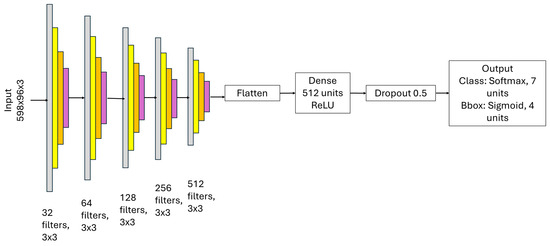
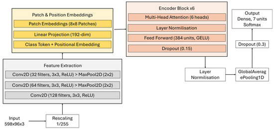
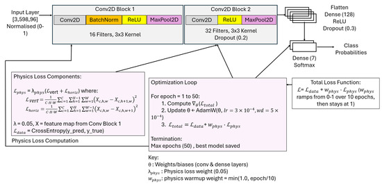
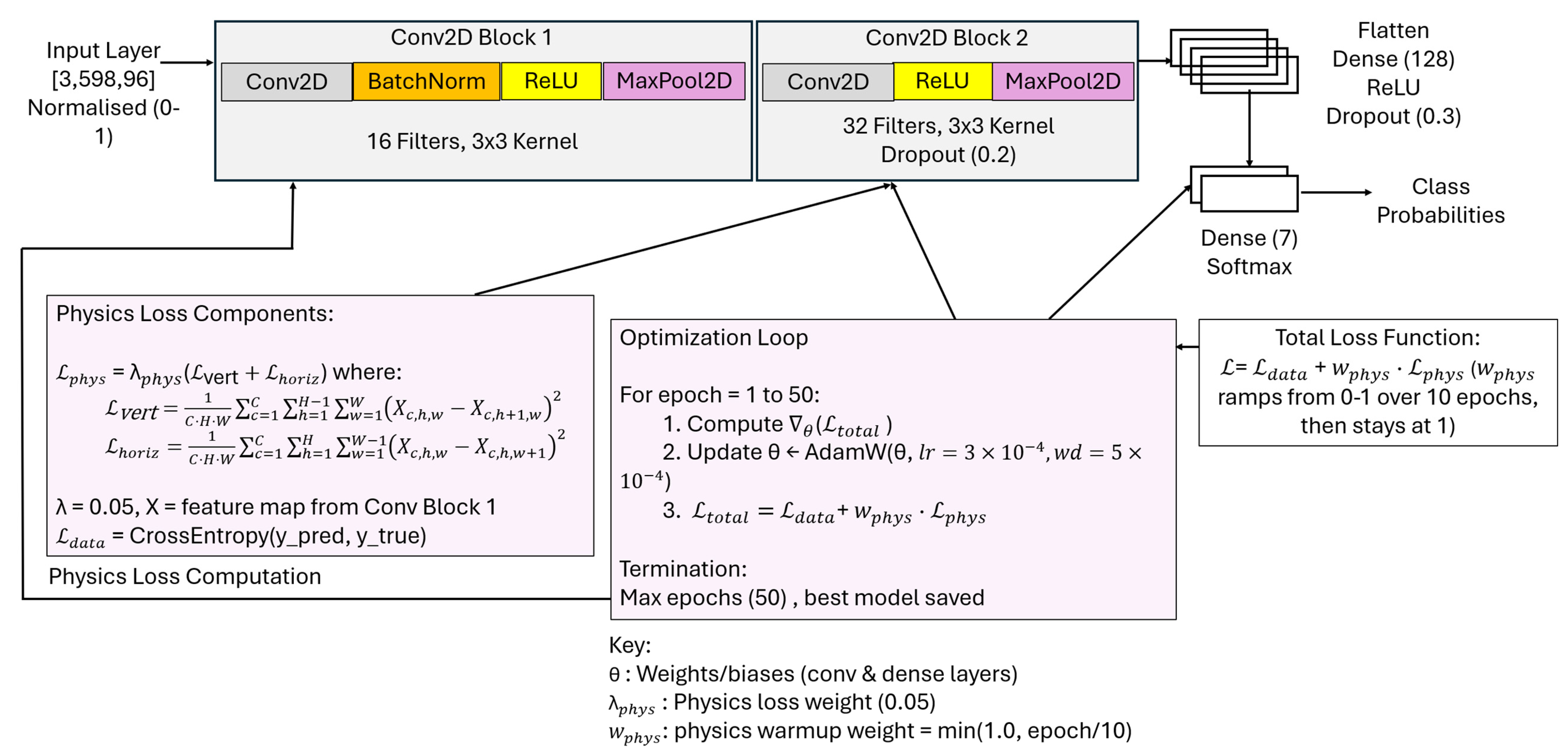
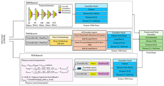
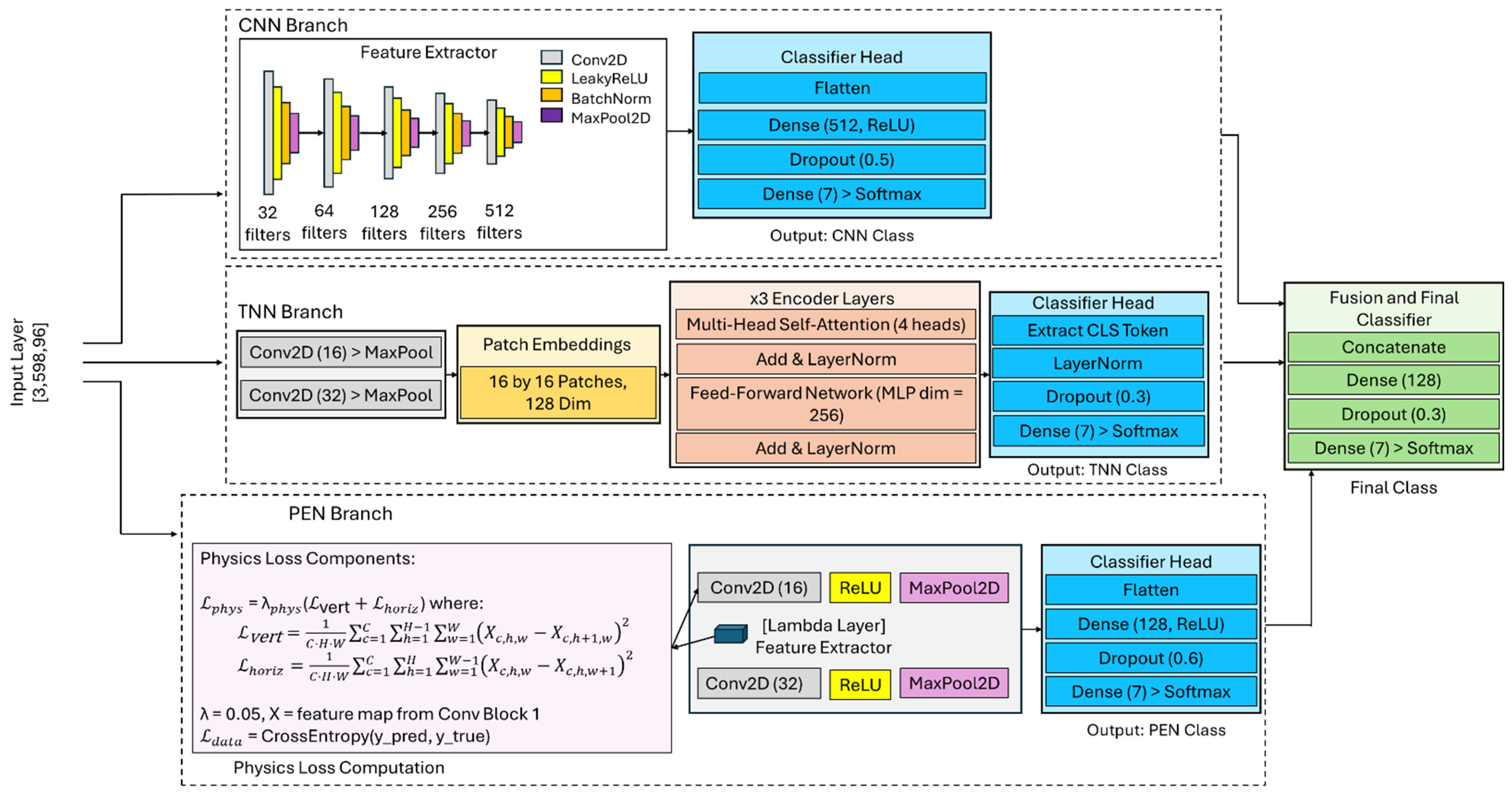
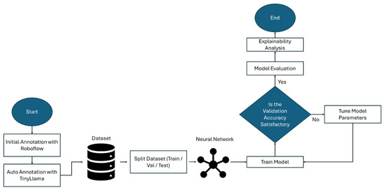
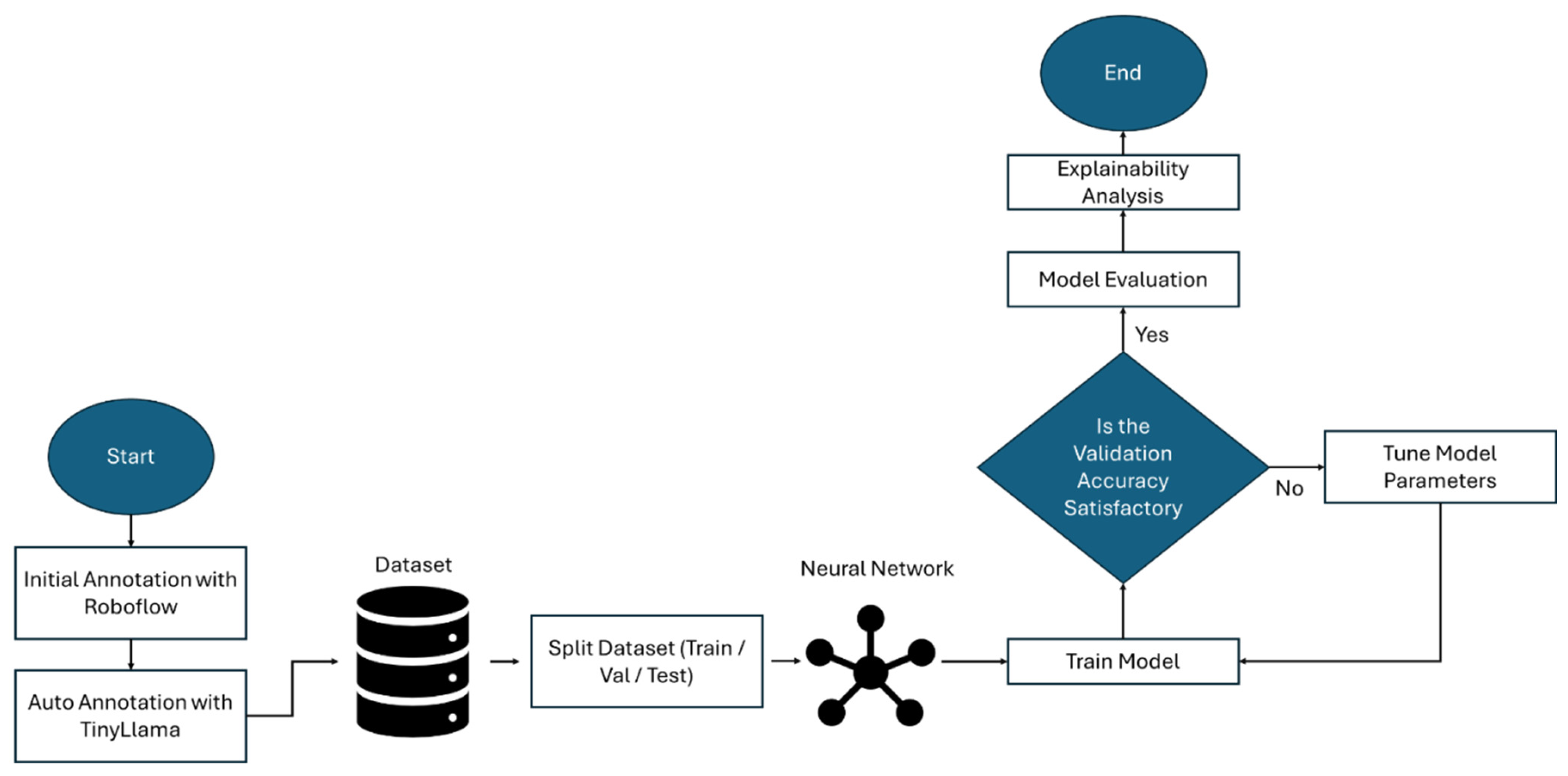
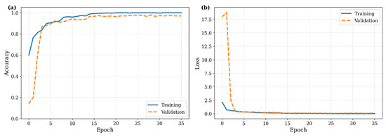
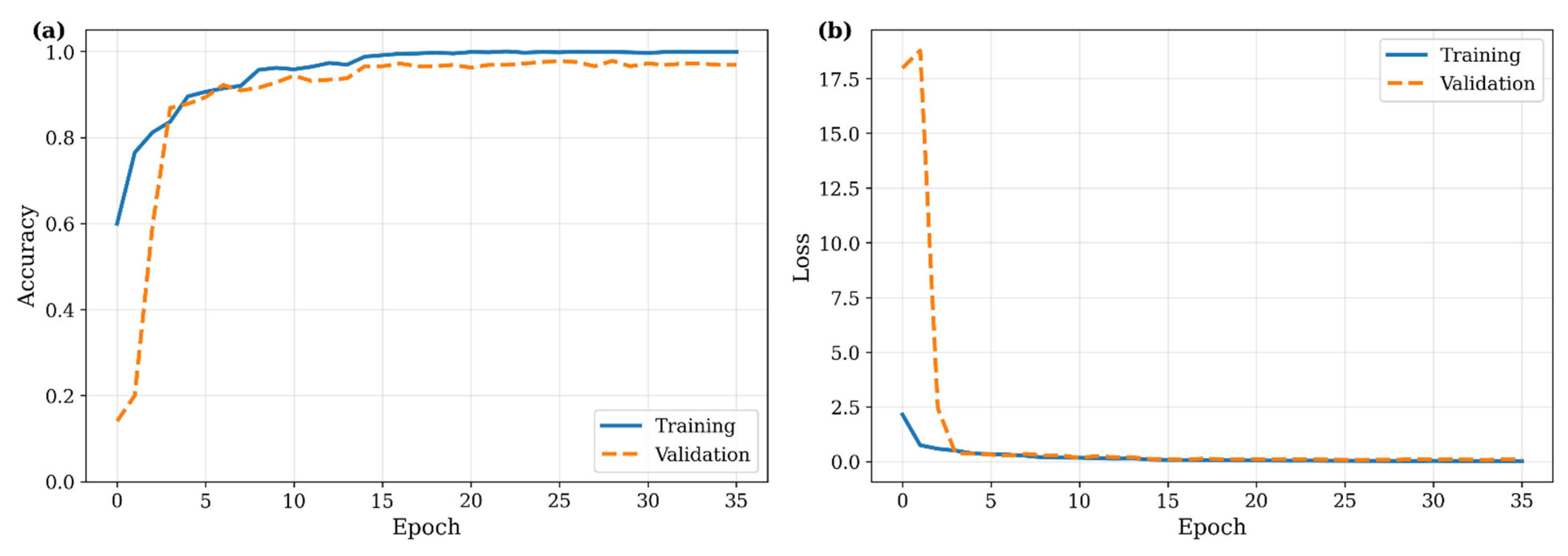
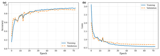
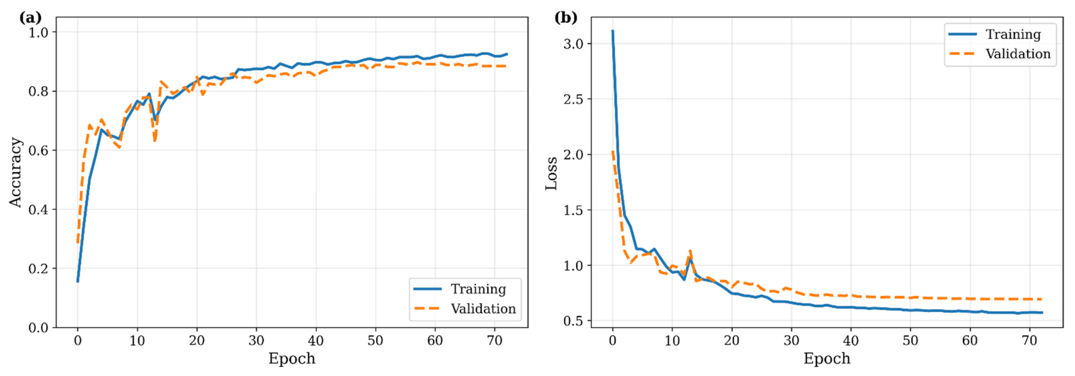
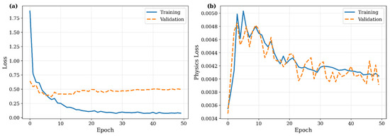
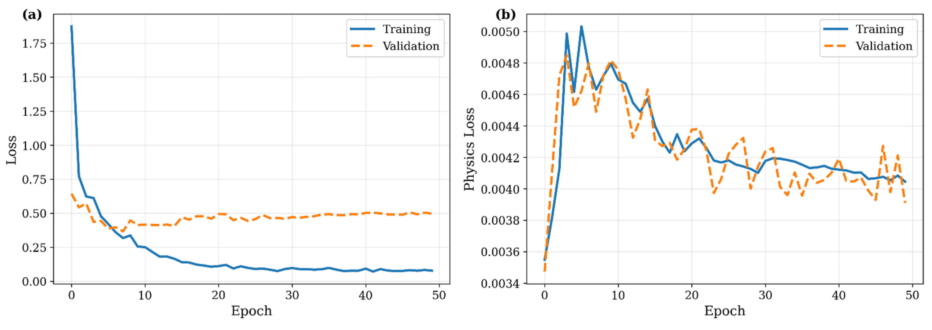
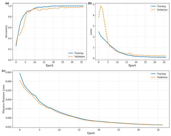
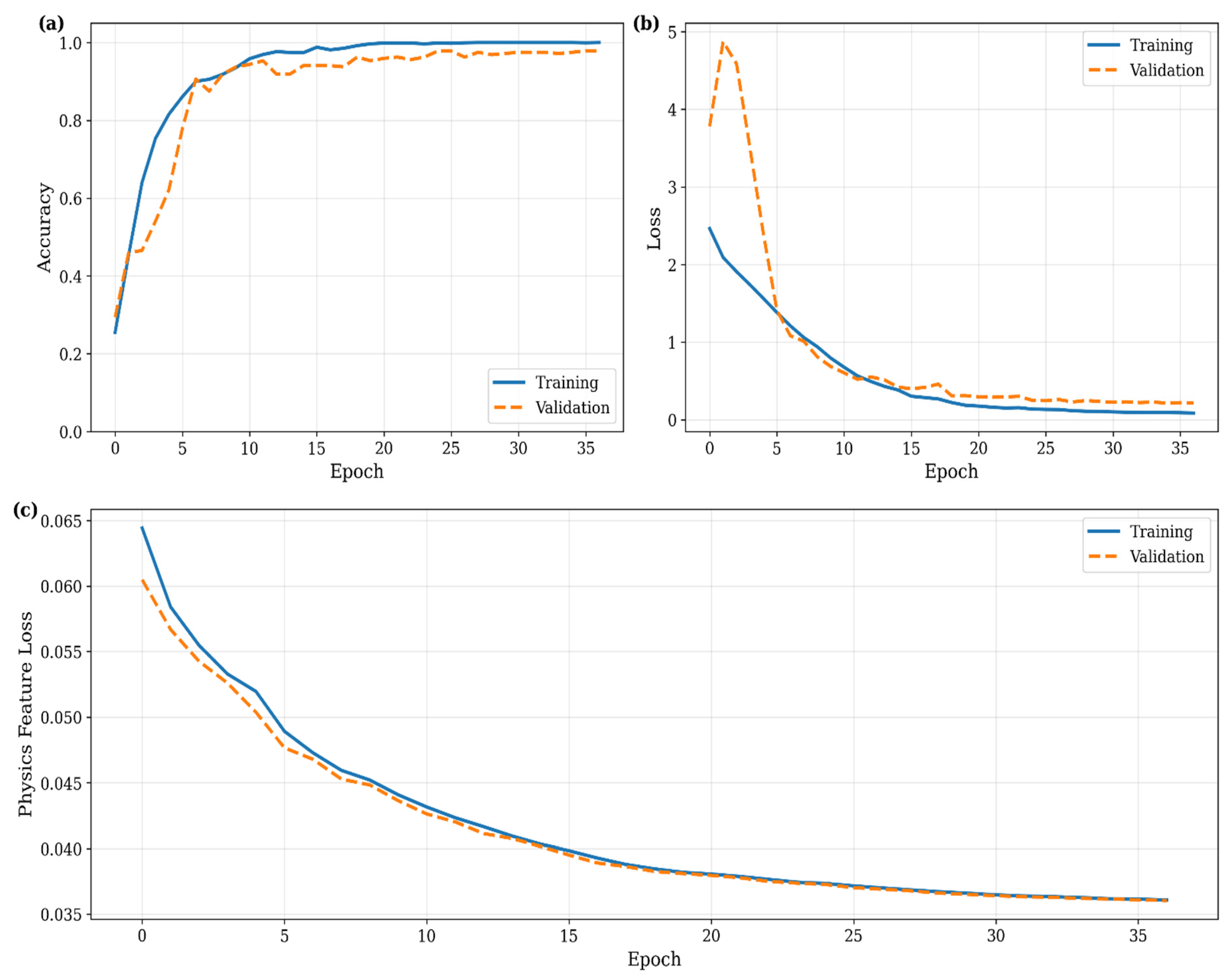
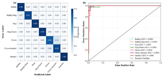
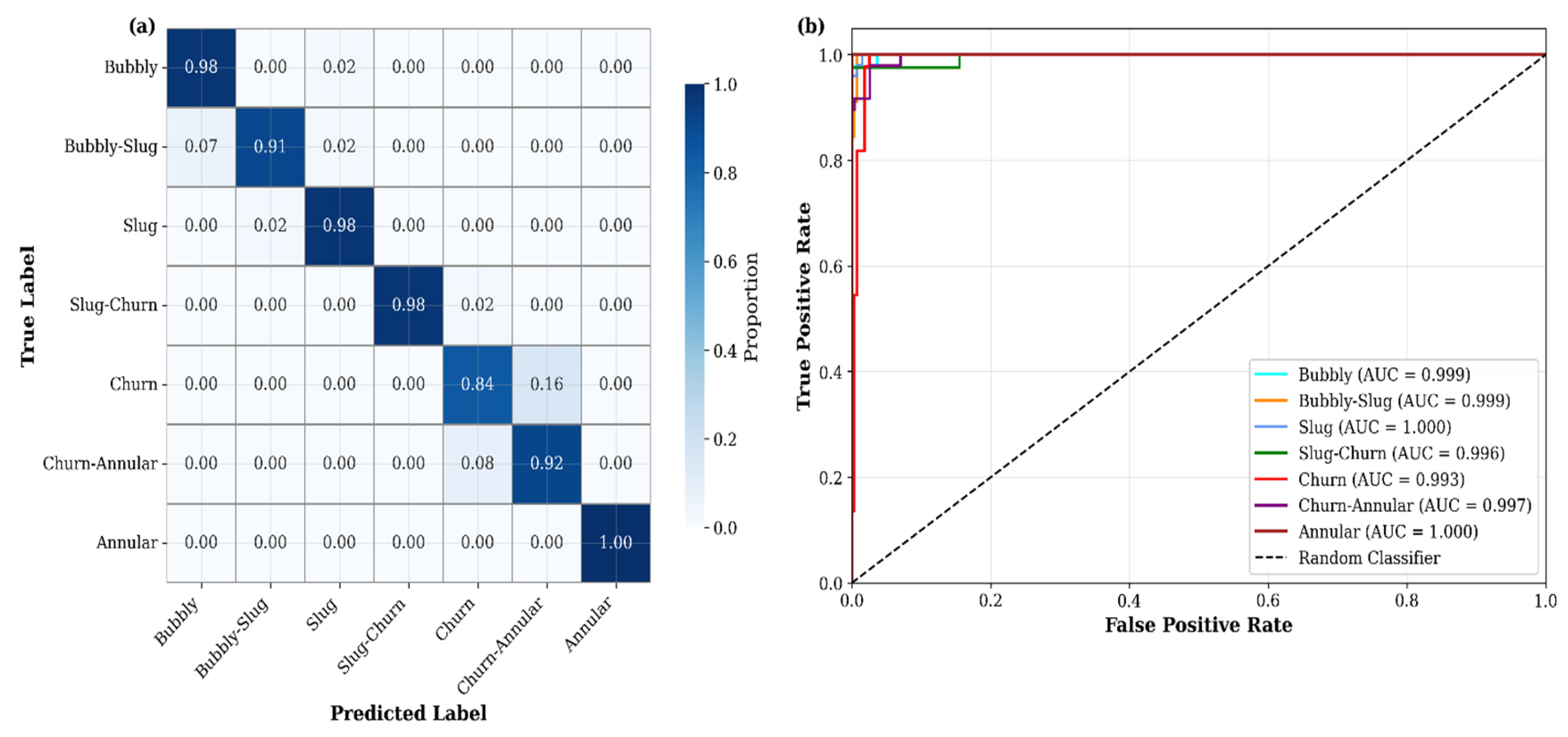
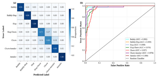
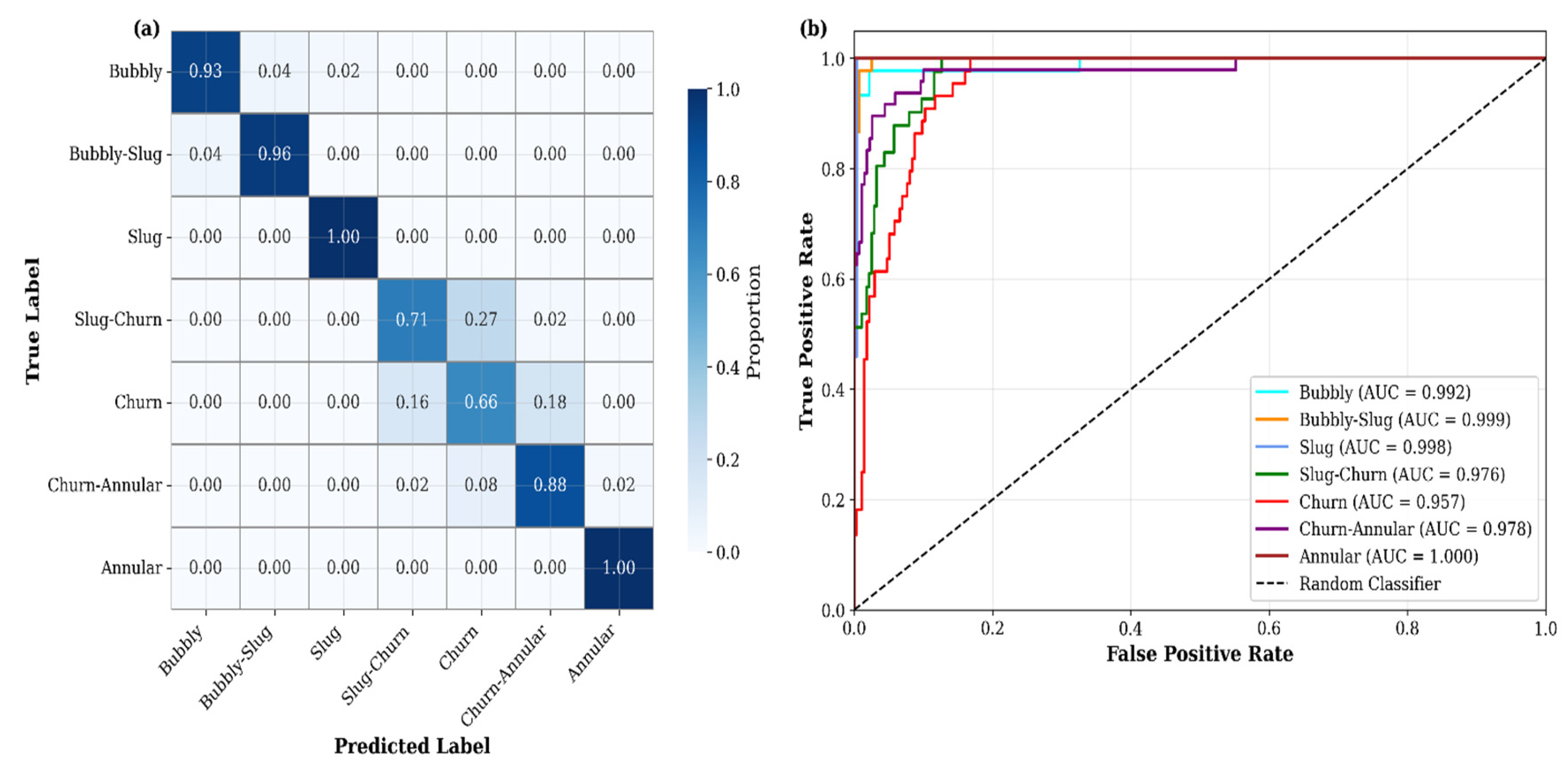
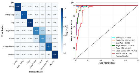
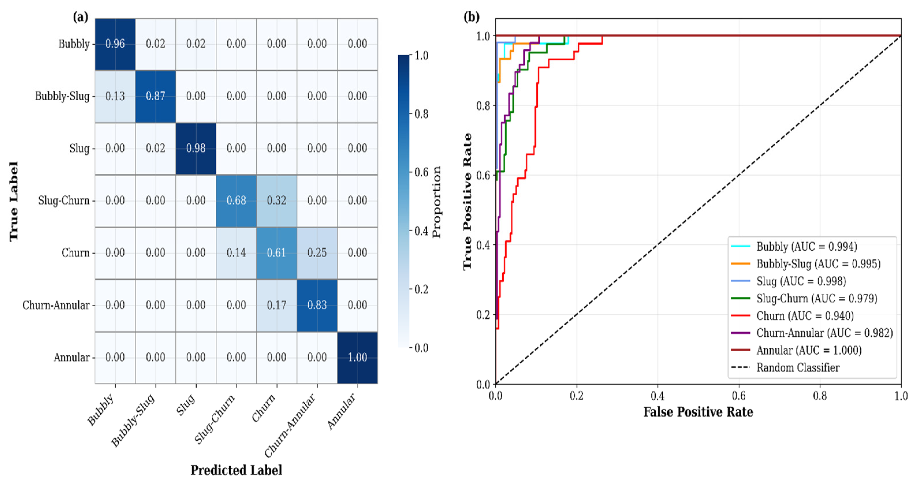
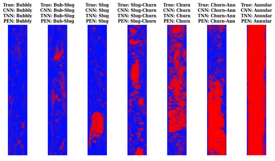
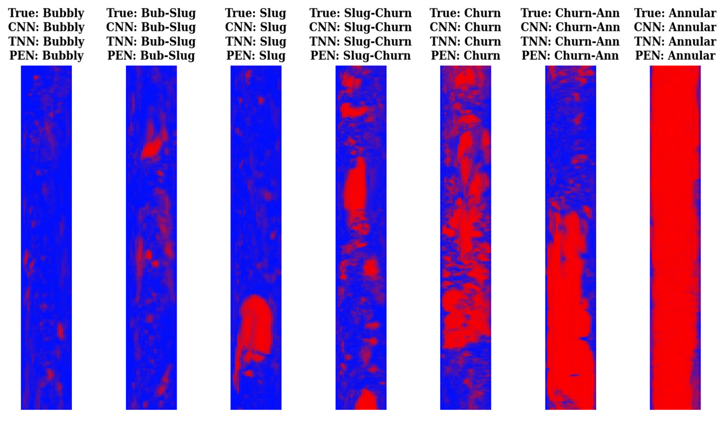
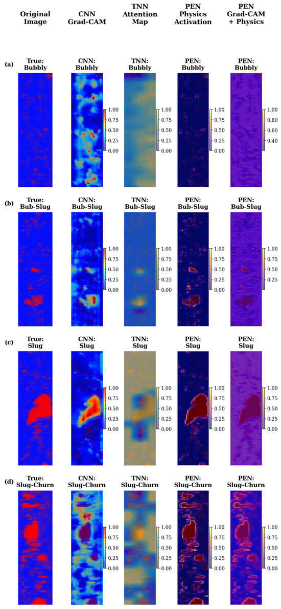
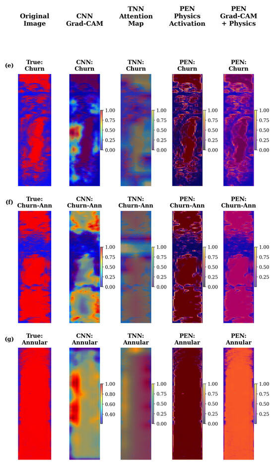
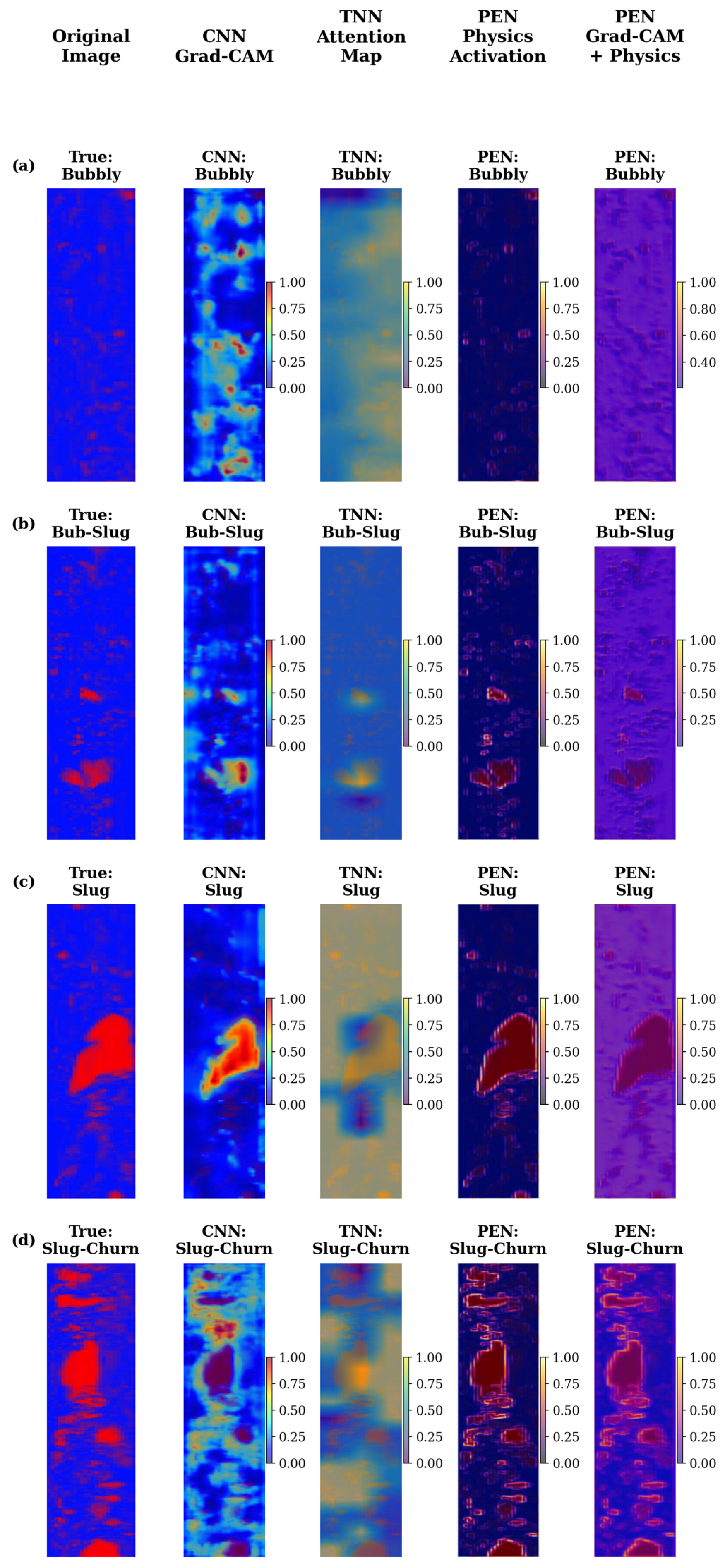
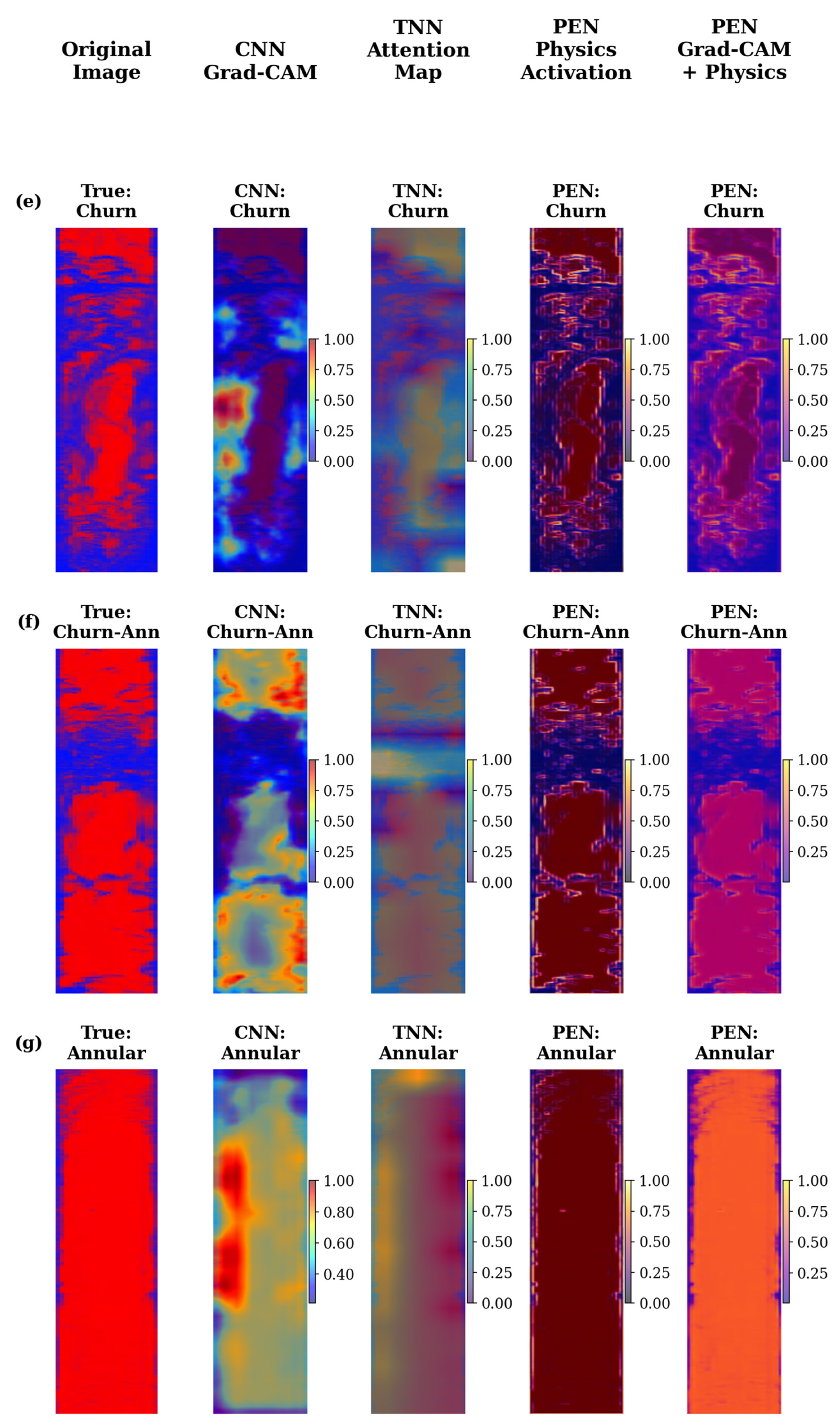
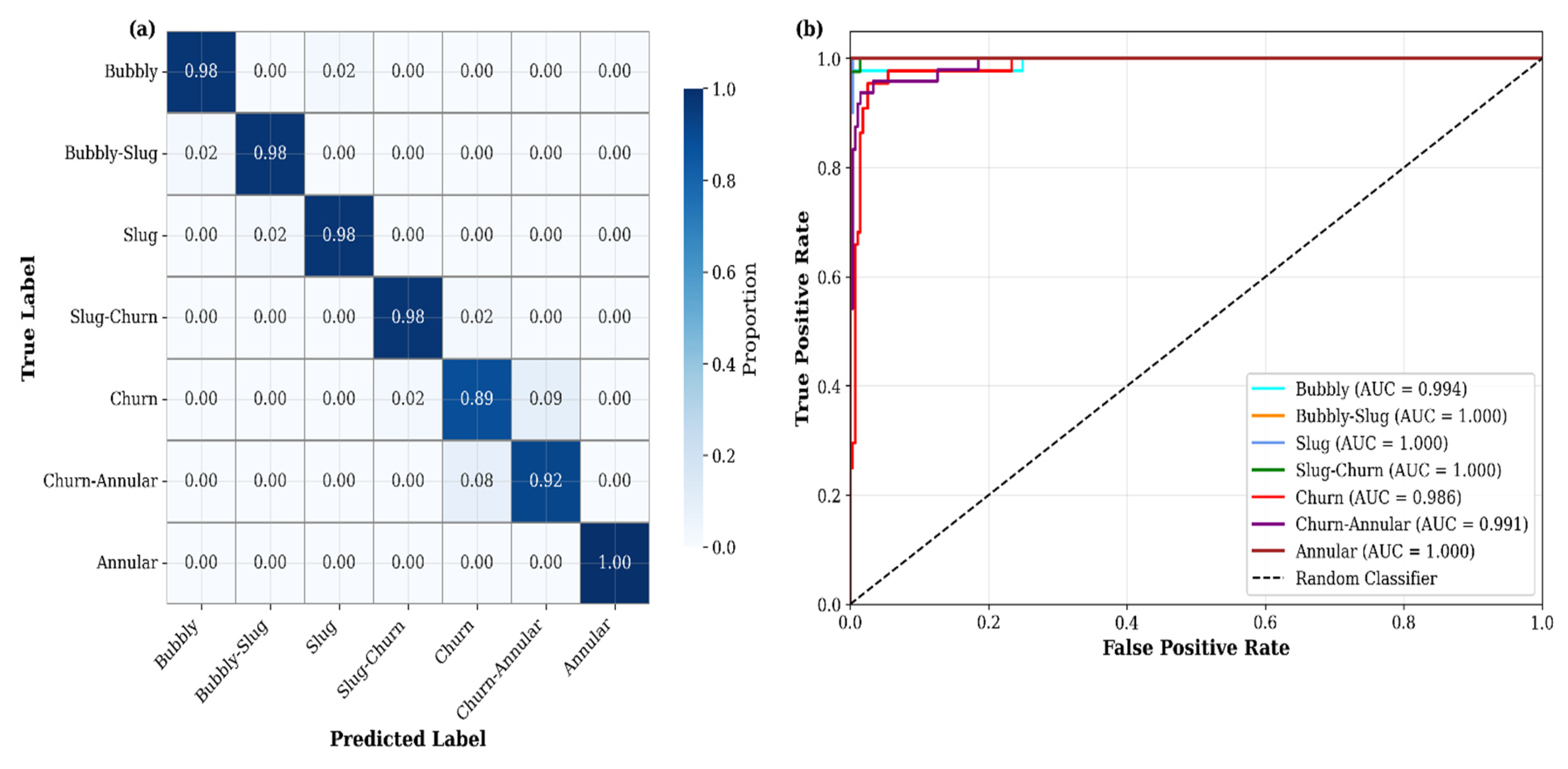
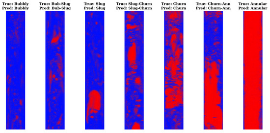
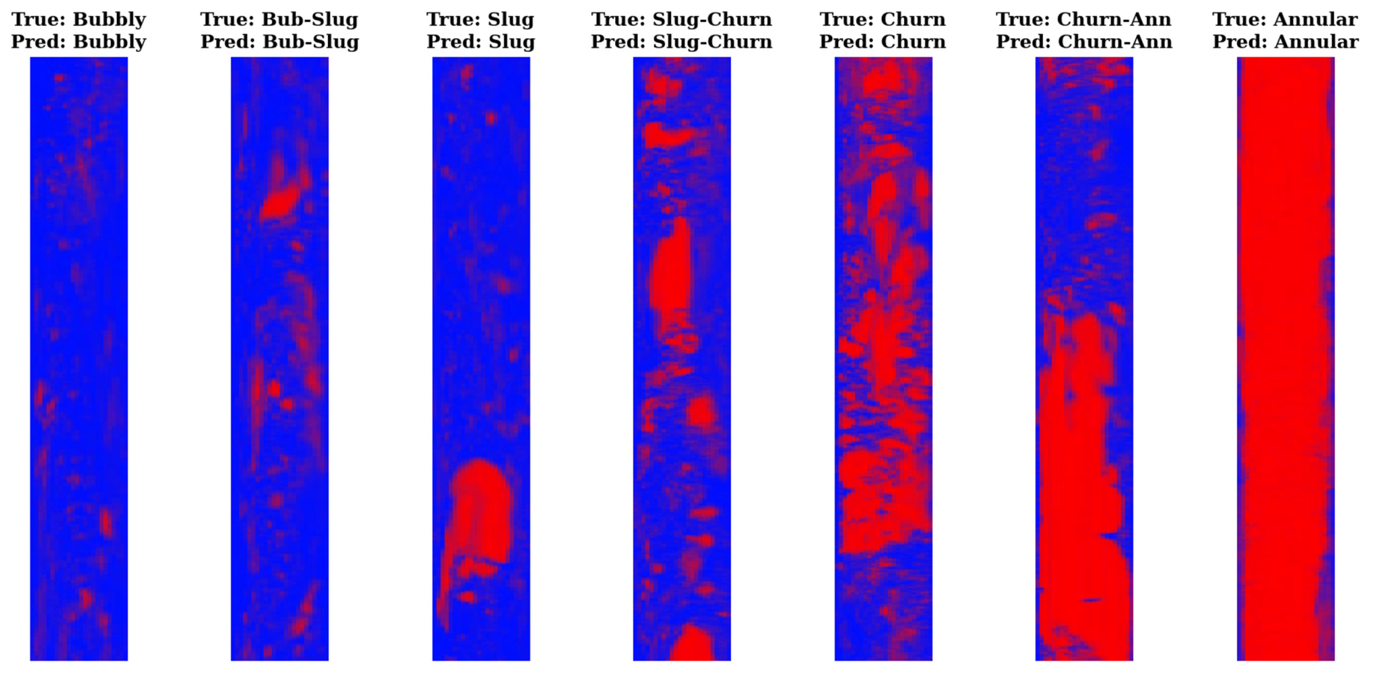
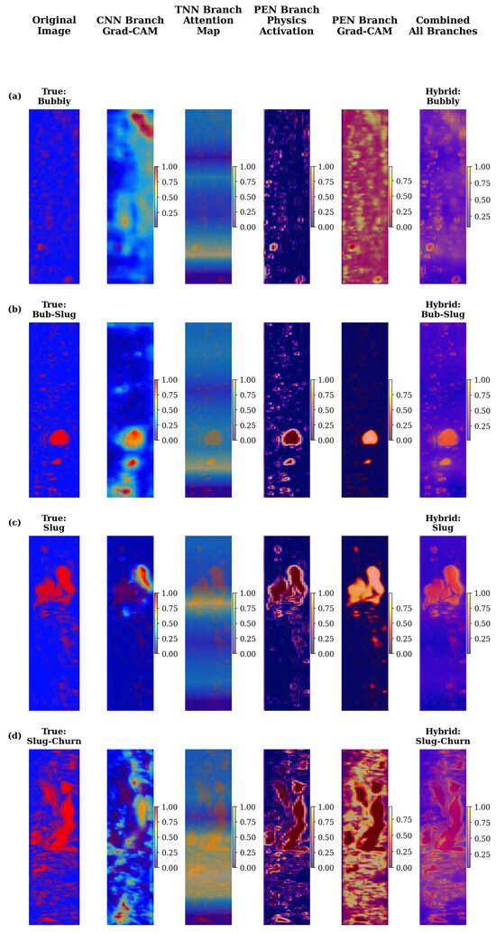
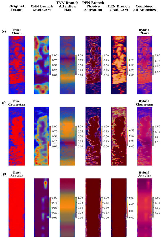
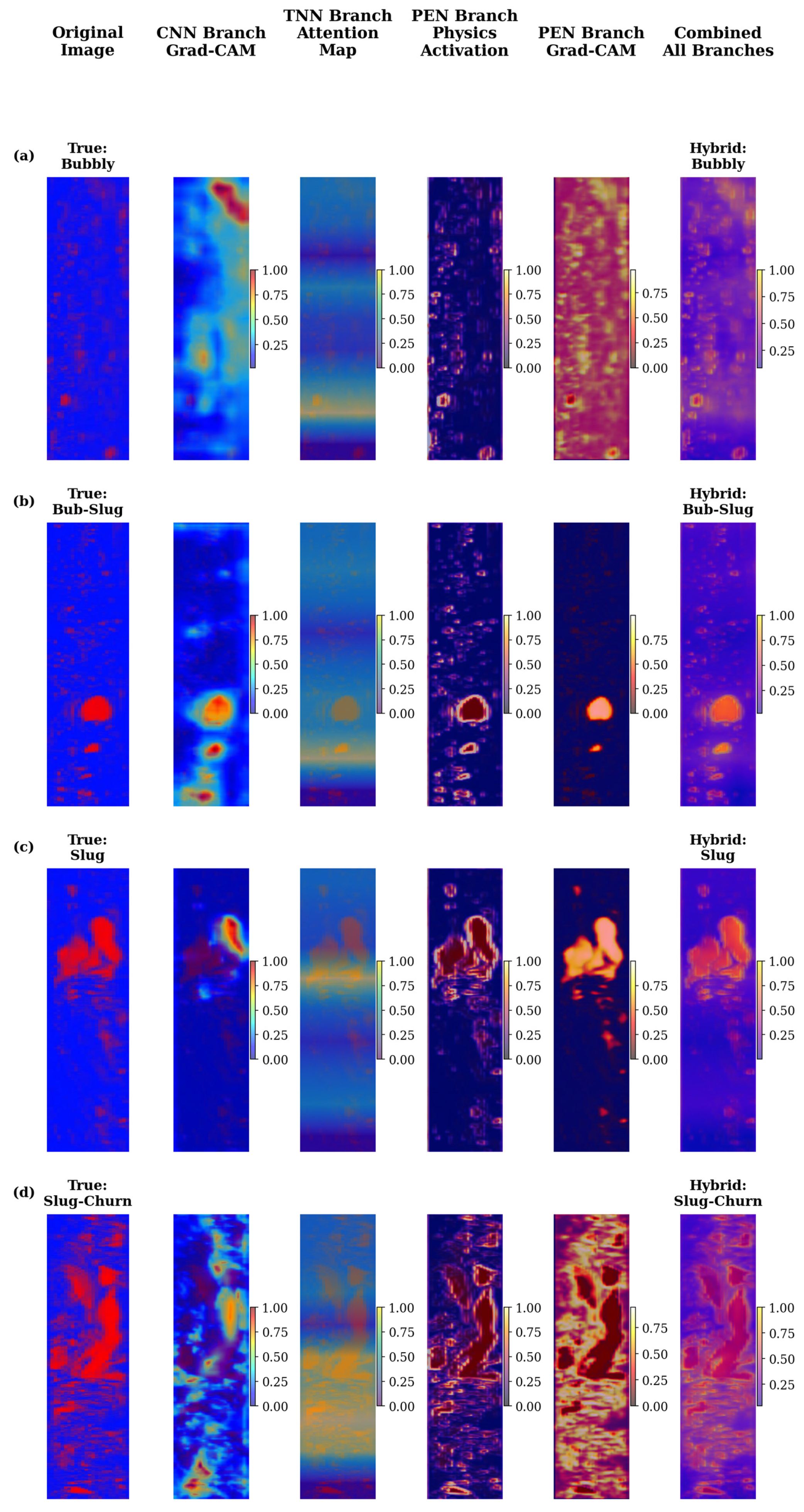
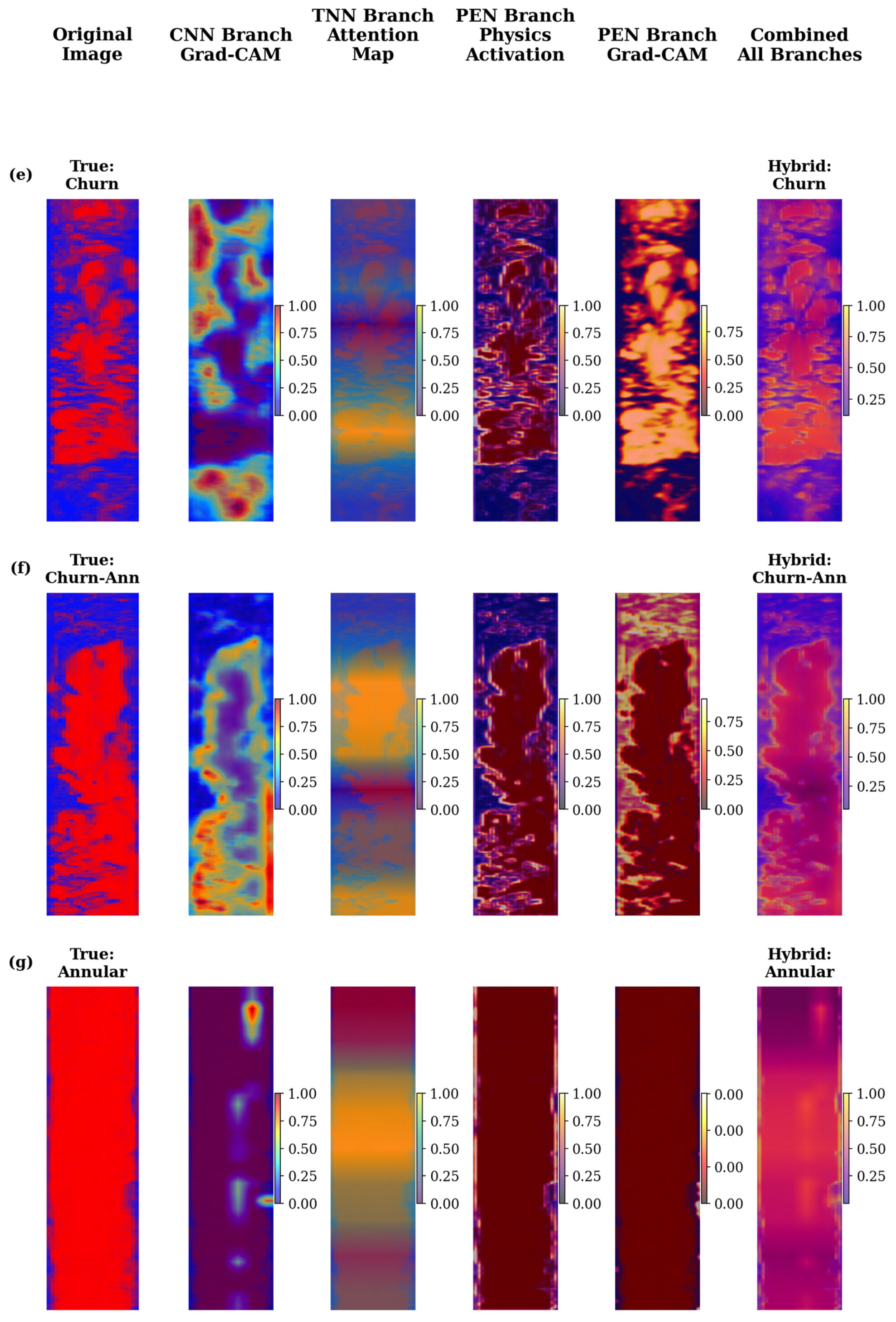
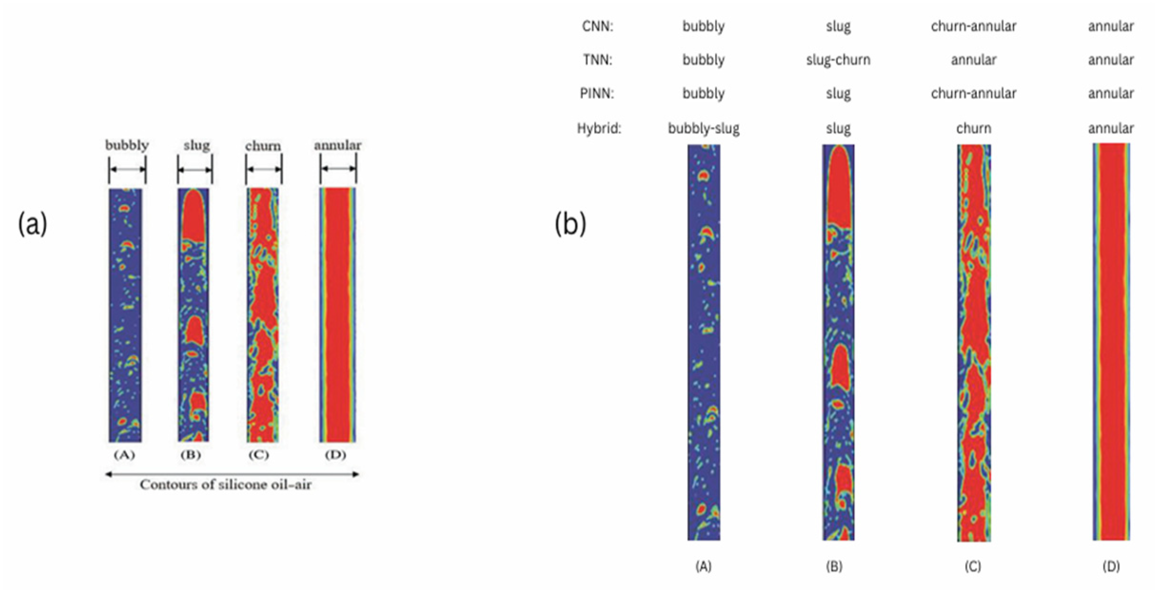
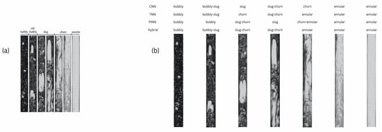
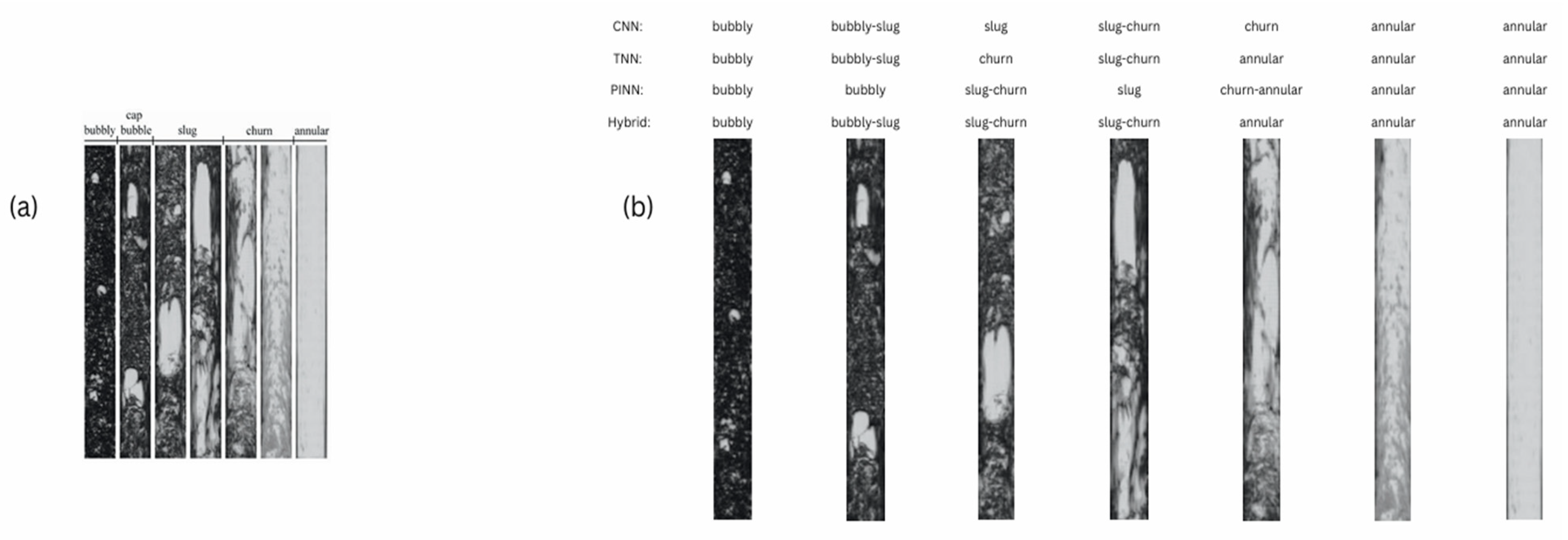

Disclaimer/Publisher’s Note: The statements, opinions and data contained in all publications are solely those of the individual author(s) and contributor(s) and not of MDPI and/or the editor(s). MDPI and/or the editor(s) disclaim responsibility for any injury to people or property resulting from any ideas, methods, instructions or products referred to in the content. |
© 2026 by the authors. Licensee MDPI, Basel, Switzerland. This article is an open access article distributed under the terms and conditions of the Creative Commons Attribution (CC BY) license.