


Abstract
Computational fluid dynamics methods range from Reynolds-Averaged Navier–Stokes (RANS) simulations to Direct Numerical Simulations (DNSs). RANS offers low computational cost at the expense of accuracy, while DNS provides high accuracy but at a prohibitive cost. The aim of this study is to evaluate whether multi-fidelity neural networks can learn a corrective mapping from RANS to DNS for a small canonical dataset and to determine how training-set composition and model architecture influence generalisation across geometries. In this study, multi-fidelity neural networks for data fusion between low-fidelity RANS and high-fidelity DNS data were applied to turbulent flow (Re = 5600) over parameterised periodic hills, defined by a geometry parameter characterising the steepness ratio. The inputs to the models were the coordinates and the corresponding RANS velocity components, and the outputs were the DNS velocity components, with data from both fidelities mapped onto the same mesh. Both a single-branch and a two-branch architecture were considered. Generalisability was assessed within a small dataset of five periodic hills defined by different values of the geometry parameter (0.5, 0.8, 1.0, 1.2, 1.5). Both model architectures were trained on data from different combinations of the geometry parameter to evaluate interpolation and extrapolation capabilities. Both networks successfully corrected RANS flow fields for unseen geometries in interpolation regimes. When interpolating, the single-branch architecture achieved more than a 69% reduction in error, while the two-branch architecture achieved more than a 60% reduction, with both improving key flow features such as recirculation zones and jet structures. A key finding is that the single-branch architecture consistently outperformed the two-branch formulation, particularly in low-data regimes. The results show that multi-fidelity neural networks can improve RANS predictions using small datasets and simple inputs, provided that the training set spans the relevant geometric space. As the model does not require the geometry parameter as an explicit input, it is applicable to geometries lacking straightforward parameterisation. The demonstrated advantage of the single-branch architecture highlights the importance of architectural simplicity when training data is limited.
1. Introduction
Computational fluid dynamics (CFD) is widely used in the design and analysis of fluid-contacting devices in fields such as turbomachinery, aerospace, automotive engineering and biomedicine. CFD applies numerical methods to approximate solutions for the conservation of mass and momentum by solving the Navier–Stokes equations. In many practical applications, fluid flow is turbulent, which involves chaotic behaviour due to the formation and interaction of swirls known as eddies. For such flows, depending on the desired level of accuracy and computational expense, different modelling approaches can be employed. The three main classes of Navier–Stokes solvers, in order of increasing fidelity, are Reynolds-Averaged Navier–Stokes (RANS), Large Eddy Simulation (LES), and Direct Numerical Simulation (DNS). DNS directly resolves the Navier–Stokes equations in three dimensions and time, capturing all spatial and temporal turbulence scales without relying on turbulence models [1], while RANS computes only the time-averaged flow field and relies on turbulence models to find the Reynolds stresses and close the system of equations, approximating the effects of turbulence. LES involves explicitly solving eddies larger than the grid scale while modelling the effect of the small scale eddies using a sub-grid-scale turbulence model.
In several practical fluids applications, designs are commonly evaluated using CFD as it offers a simple, cheap and reproducible method compared to bench tests. While RANS methods are commonly used in simulating fluid flow in turbulent applications, due to their lower computational cost [2,3,4], they can be inaccurate for transitional flows [5]. DNS is the most accurate way of resolving transitional and turbulent flows, but it is so computationally expensive that, even with very powerful computers, it can only be applied to relatively simple geometries or low Reynolds number flows, requiring meshes and time steps small enough to capture the smallest vortices.
In recent years, machine learning has offered a new paradigm for solving scientific problems using data and physical knowledge due to its ability to learn complex patterns and functions from data. One such scientific application is CFD, where machine learning presents an opportunity to reduce computational cost, improve accuracy and replace mesh-based methods. Machine learning can be used to discover context-specific patterns in fluid data that have been obtained from simulations or experiments, with applications in weather modelling [6], wind energy [7] and aerodynamics [8]. Machine learning has been used for developing surrogates, solving of inverse problems, flow control, and the enhancement of numerical solvers [9].
Multi-fidelity machine learning is one such application and involves leveraging data from different levels of fidelity, combining the abundance of low-fidelity data with the accuracy of high-fidelity data. Multi-fidelity machine learning has been applied in CFD applications where low-fidelity and high-fidelity solutions exist, with an accuracy–cost trade-off between the two. In CFD, multi-fidelity modelling can be grouped into three categories: discovering closure terms, data assimilation and data fusion. Various authors have employed multi-fidelity methods to learn approximations between RANS/LES and DNS for improved turbulence closure in the form of either improving RANS solvers by correcting the anisotropic stress tensor [10,11,12] or improving LES by learning sub-grid scale stresses [13,14,15,16]. Variational data assimilation has been used for inverse problems in discovering terms in RANS solvers or for forward problems for reconstructing RANS flow fields [17,18,19]. Although these approaches improve low-fidelity solutions, they require modifications to the low-fidelity solver itself, either by altering closure terms/coefficients or by constraining the solution using sparse high-fidelity data. These methods are therefore dependent on altering the CFD codes, meaning they are not straightforward to implement in practice, and cannot be applied to pre-existing simulation results.
In contrast to solver-based approaches, data-fusion methods enhance the fidelity of simulation outputs by integrating low and high-fidelity datasets during model training, without modifying the underlying CFD solver. He et al. employed multi-fidelity neural networks to approximate the relationship between Mach number and angle of attack, and lift and drag coefficients for airfoils. Their model was trained on 120 low-fidelity cases derived from an Euler solver and 24 high-fidelity cases obtained from SST RANS simulations [20]. Similarly, Zhang et al. [21] and Liao et al. [22] applied multi-fidelity machine learning to aerodynamic shape optimisation, using coarse mesh RANS solutions as low-fidelity data (over 120 cases) and fine mesh simulations as high-fidelity data (over 60 cases). Zhang et al. used geometric parameters as inputs to a feedforward neural network, whereas Liao et al. employed airfoil images as inputs to a convolutional neural network (CNN). Sánchez-Moreno et al. extended this approach to nacelle design, using multi-fidelity data fusion to correct drag predictions across varying design parameters. Their low-fidelity data was based on Euler equation solutions, while high-fidelity data was obtained from RANS simulations [23]. More recently, Li et al. proposed a multi-fidelity graph neural network (GNN) to approximate mappings from 3D spatial coordinates and blade parameters in turbomachinery to pressure, temperature, and velocity fields. In their framework, low-fidelity data was generated from low-fidelity simulations ignoring the effects of turbulence, and high-fidelity data from SST RANS simulations [24]. Among these studies, Liao et al. [22] adopted a transfer learning-based multi-fidelity strategy, while the others [20,21,23,24] implemented or adapted the composite multi-fidelity neural network architecture originally proposed by Meng et al. [25]. Notably, most applications of multi-fidelity neural networks in CFD focus on improving predictions of derived flow quantities such as lift and drag coefficients [20,21,22,23], rather than reconstructing full flow fields. To date, only one study has demonstrated the use of multi-fidelity data fusion to enhance predictions of complete flow fields [24].
Global parameters such as drag or lift coefficients, pressure gain or drop, efficiency and haemolytic index are commonly calculated from flow fields as they make design optimisation easier. This is because using a single or few coefficients reduces the complexity and dimensionality of the problem. However, these only give a global evaluation of a design and ignore local features which may be important to consider. Full flow fields allow engineers and scientists to have a complete understanding of the flow and to identify more local flow features such as recirculation zones, separation, vortex formation, high shear regions and shock location. In addition, a range of global coefficients can be computed for each design case as a post-processing step.
The aim of this work was to develop and evaluate a multi-fidelity machine learning framework capable of reconstructing complete velocity fields with improved accuracy. Unlike most existing data-fusion studies, where RANS typically represents the highest fidelity level and DNS is seldom employed, this work leverages DNS directly as the high-fidelity reference to move beyond RANS-level fidelity. This study focuses on a constrained but practically relevant setting in which low-fidelity RANS data is abundant and only a small number of high-fidelity DNS cases are available. While several previous studies have adopted composite (two-branch) multi-fidelity architectures, the present work additionally evaluates their performance against a simpler and smaller single-branch alternative. Particular emphasis is placed on evaluating to what extent a multi-fidelity architecture can improve RANS predictions within a limited design space, when trained on a small dataset, unlike prior studies that often rely on more than one hundred cases in the training set. The aim is therefore not to develop a universally generalisable surrogate, but to improve RANS predictions, using a small number of DNS examples, within a limited design space. While several authors have previously included geometry parameters or representations as inputs to the neural network [21,22,23], this study investigates whether such inputs for representing the geometry are explicitly necessary when the full RANS field and coordinates are also used as inputs. Accordingly, the study intentionally omits explicit geometric parameters as inputs, in order to isolate whether geometry-dependent corrections can be learned solely from the spatial coordinates and the low-fidelity flow field. Finally, the workflow is designed to remain simple to set up and apply, lowering the barrier for adoption in practical CFD applications.
2. Method
The generalisability of multi-fidelity data fusion for learning the approximation from RANS to DNS data was evaluated in a parameterised periodic hill case study. Two multi-fidelity neural network architectures were compared for approximating between low-fidelity RANS data and high-fidelity time-averaged DNS data: the composite multi-fidelity neural network architecture, proposed in [25], and a single-branch multi-fidelity neural network. Multilayer perception (MLP)-based approaches were used instead of CNNs because CNNs require structured grid-like data in the form of a matrix or an image with regular pixel size due to the use of a sliding filter as part of the convolution operation. Furthermore, CNNs for full flow field prediction require geometric feature representation, for example, the location of boundaries, on a regular grid in the form of signed distance fields [26] or other geometry representation approaches [27].
The workflow consists of three main stages described in the following subsections: (i) data preparation (Section 2.1); (ii) multi-fidelity model set up and training (Section 2.2 and Section 2.3) (iii) conducting experiments to investigate generalisation (Section 2.4).
2.1. Dataset
The dataset used to train the model has been published by McConkey et al. for use in developing machine learning methods for corrective turbulence modelling [28]. All simulations, mesh generation, and data processing were performed by the original authors. The dataset consists of RANS simulation data from four RANS models and the corresponding DNS/LES data for each domain and flow condition for various CFD benchmark problems.
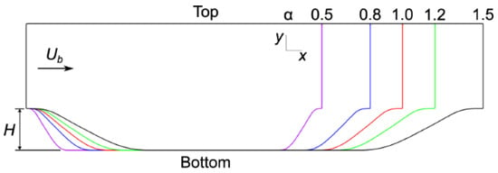
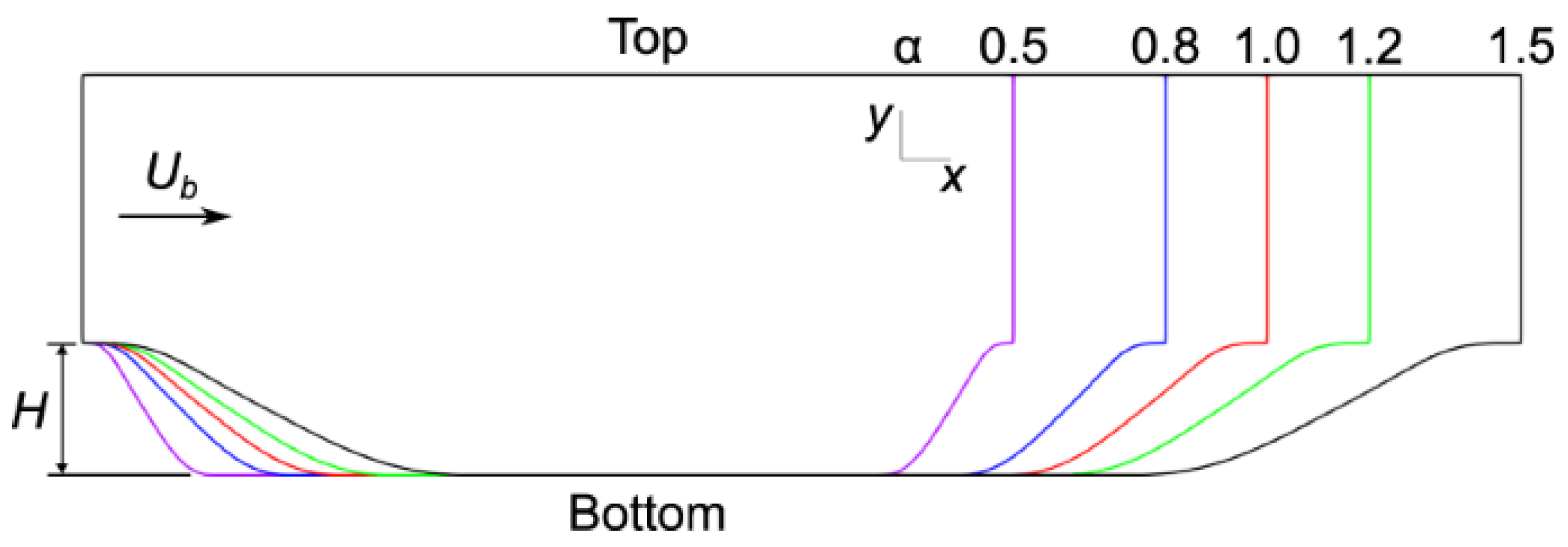
The two-dimensional periodic hill geometry (Figure 1) was selected as the benchmark case for this study. This configuration is widely used for assessing turbulence model performance and analysing separated flows [29,30]. The periodic hill provides a controlled canonical setting in which key flow features, such as boundary layer separation, vortex formation, and reattachment, are observed. The periodic hill reflects flow behaviour encountered in a range of engineering systems, including aerodynamic surfaces, turbomachinery blades, curved ducts, pipes, and diffusers [31]. Its broad applicability makes it a common benchmark for evaluating multi-fidelity modelling strategies.
Figure 1.
Geometries of 5 periodic hills parameterised by the steepness ratio = 0.5, 0.8, 1.0, 1.2, 1.5 (Taken from [28]).
For the periodic hill configuration considered here, the low-fidelity data was generated through the SST RANS model on meshes of approximately 15,000 elements, and high-fidelity data was generated through DNS simulations on very fine meshes of approximately 40 million elements. The flow regime is turbulent with a Reynolds number of 5600. As described in the dataset documentation, cyclic boundary conditions in the streamwise direction and no-slip conditions on the solid walls were applied. As documented in McConkey et al., the DNS fields were time-averaged and subsequently mapped onto the equivalent coarser RANS mesh for each geometry. The mapping procedure was implemented by the authors by evaluating the DNS solution at the RANS cell centres. This approach ensures that both fidelities share the same spatial locations, which is required for point-wise supervised learning. Although the downsampling from the DNS mesh inevitably smooths some small-scale turbulent structures, the main flow features and mean quantities are preserved. The mapped DNS fields therefore still provide suitable high-fidelity labels for multi-fidelity training without introducing the difficulties associated with unaligned meshes in machine learning.
The x-coordinates (x), y-coordinates (y), horizontal velocity from RANS () and vertical velocity from RANS () constitute the input to the neural network with 4 input nodes corresponding to each of these features. The horizontal velocity from DNS () and vertical velocity from DNS () constitute the ground truth for the neural network with 2 output nodes.
The data for all periodic hills ( = 0.5, 0.8, 1.0, 1.2, 1.5) were normalised globally using min–max normalisation (Equation (1)) for both the input and output variables.
2.2. Multi-Fidelity Model Architecture
Two multi-fidelity architectures are considered and compared in this study: a two-branch composite architecture and a single-branch architecture. Both models are based on the assumption that high-fidelity functions () can be modelled as functions of the corresponding low-fidelity function () and coordinates of the domain (x).
2.2.1. Two-Branch Composite Architecture
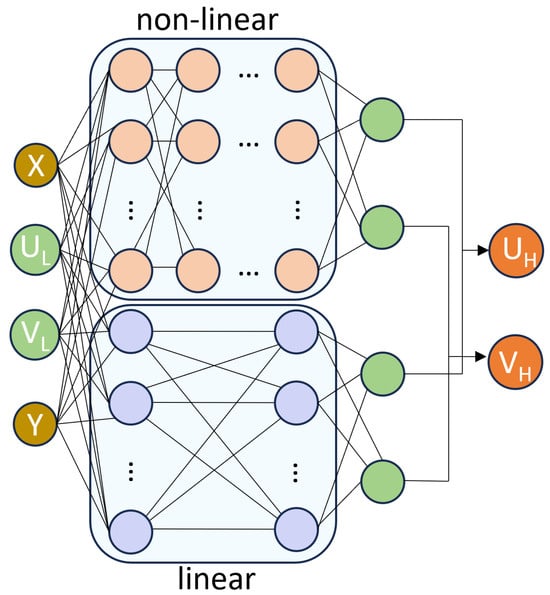
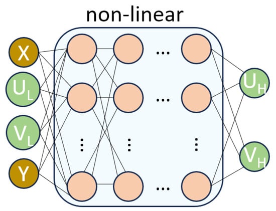
In this architecture, the relationship between low and high-fidelity can be represented by the sum of a linear function () and a non-linear function () of the low-fidelity function and coordinates of the system (Equation (2)). In the context of neural networks, this can be constructed as two branches: the linear branch and the non-linear branch. The non-linear branch has non-linear activation applied to each layer, while the linear branch has no activation. Tanh activation was applied after each layer in the non-linear branch.
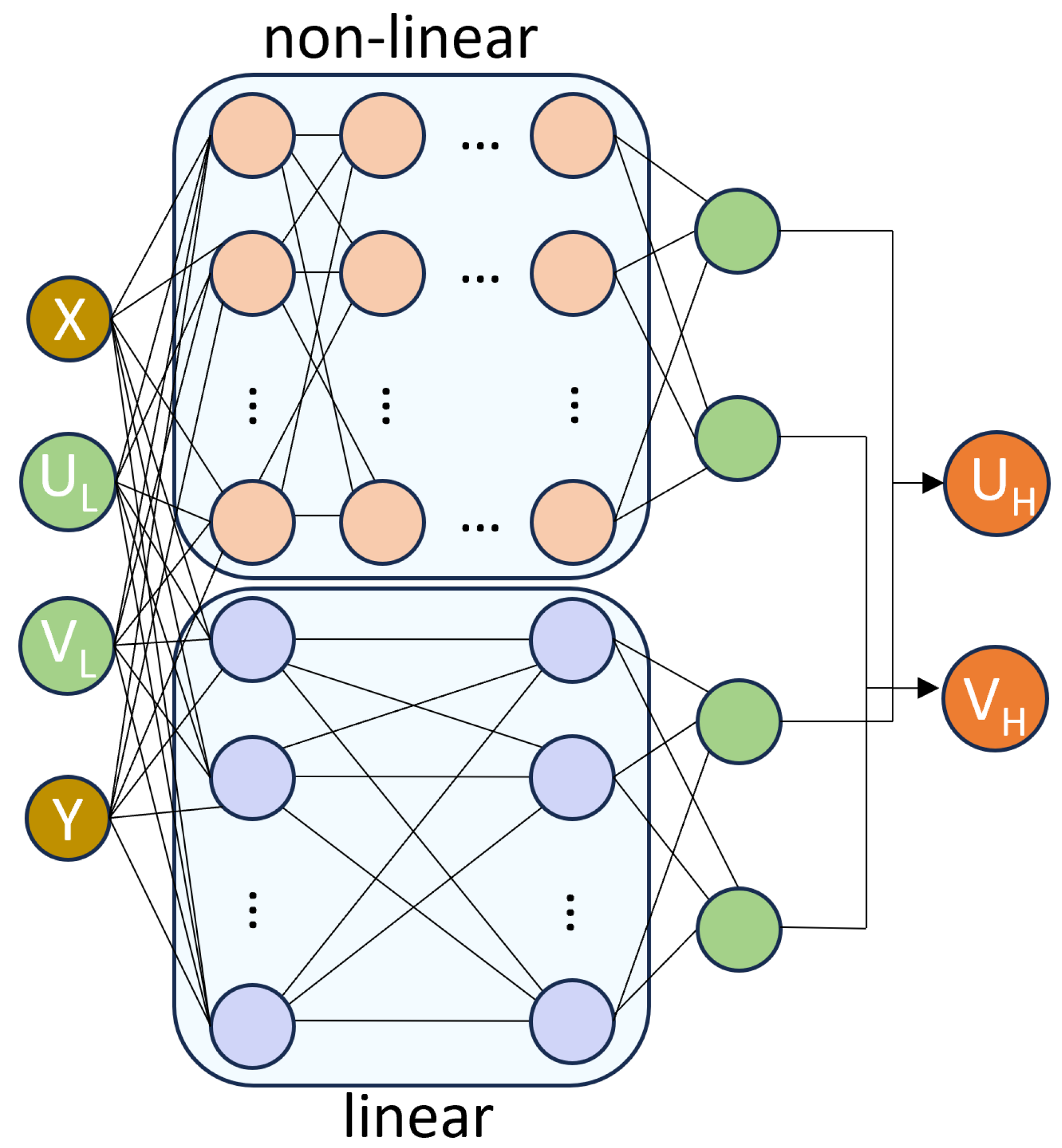
The original model by Meng et al. [25] also consists of a low-fidelity approximator which is used to map the low-fidelity data on the same points as those available in the high-fidelity dataset, before learning the approximation from low to high-fidelity. This is a requirement for cases where the low-fidelity and high-fidelity data are from different meshes. In the CFD context, an example would be of low-fidelity data from RANS simulations and high-fidelity data from DNS simulations, both of which require different mesh sizes based on the solver. In the dataset used in this paper, the RANS and DNS solutions have already been mapped onto an identical mesh, thereby making the use of the low-fidelity approximator redundant. For this application, the multi-fidelity architecture has been adapted to learn the mapping from coordinates (x, y) and low-fidelity velocity components (, ) to high-fidelity velocity components (, ) (see Figure 2).
Figure 2.
Two-branch multi-fidelity network architecture for learning approximation from x and x coordinates, and low-fidelity horizontal () and vertical () velocities to high-fidelity horizontal () and vertical () velocities. The non-linear branch has non-linear activation after each layer and the linear branch has no activation. The outputs from each branch are summed to give the output of the model.
2.2.2. Single-Branch Architecture
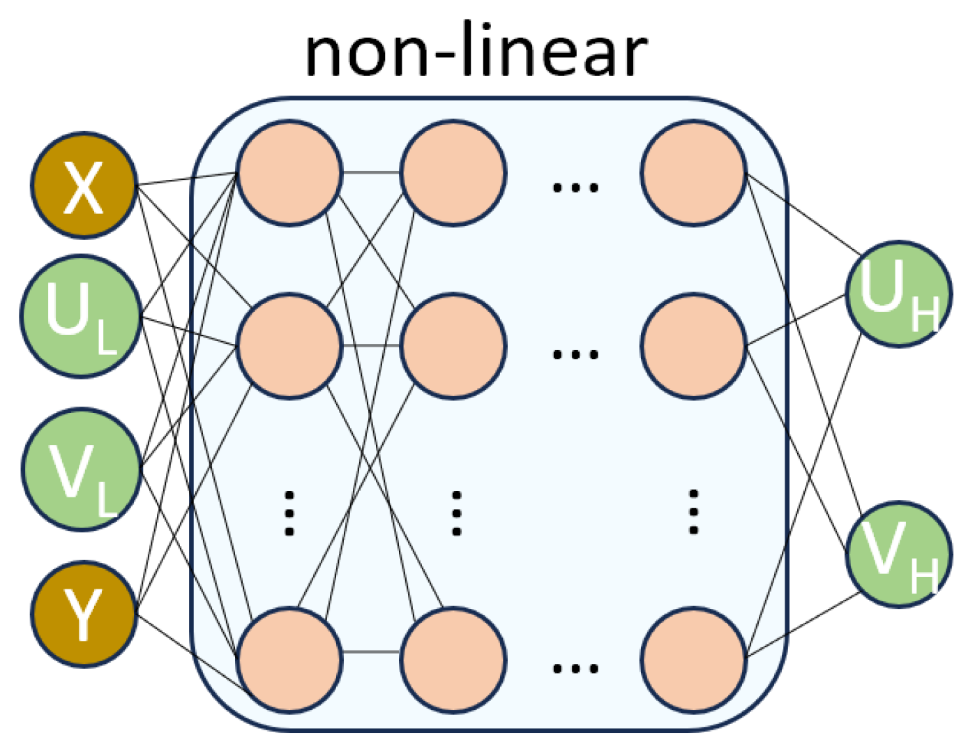
Similarly, the single-branch approach also maps the coordinates (x, y) and low-fidelity velocity components (, ) to high-fidelity velocity components (, ). This is a simplification from the two-branch architecture and only has one non-linear branch (see Figure 3). The motivation behind evaluating this simpler architecture is to investigate whether the additional linear and nonlinear decomposition employed in the composite multi-fidelity formulation offers a meaningful advantage over a more straightforward network architecture for learning the mapping between RANS and DNS solutions, for a relatively small dataset. As this architecture only has non-linear layers, tanh activation was applied to each layer.
Figure 3.
Single-branch multi-fidelity network architecture for learning approximation from x and y coordinates, and low-fidelity horizontal () and vertical () velocities to high-fidelity horizontal () and vertical () velocities. Non-linear activation is applied after each layer.
For both architectures, Glorot initialisation was used and the models were trained with the Adam optimiser for 5000 epochs followed by quasi-newton optimiser L-BFGS for 100 epochs. This two-stage approach is commonly used with PINNs. The first-order Adam optimiser was used to rapidly explore the parameter space and obtain a suitable starting point and the second-order quasi-Newton optimiser, L-BFGS, was applied to achieve smoother convergence and lower final training loss. The models were trained to minimise the sum of the L2 loss between the predicted velocities () and DNS ground truth velocities () (Equation (3)). No specific anti-overfitting techniques such as dropout, regularisation or early stopping were used, as the loss curves showed that this was not required for convergence (see Supplementary Materials).
2.3. Hyperparameter Tuning
The hyperparameter tuning was performed on the two-branch architecture to optimise the model configuration. The same best configuration was then used with the single-branch architecture after removing the linear branch as ablation. The two-branch model was trained on 10,000 randomly sampled data points from the periodic hills at = 0.5 and 1.5. The data was partitioned into training and validation subsets, and the latter was used for hyperparameter tuning. The parameters assessed were: number of linear hidden layers (1 or 2); neurons per linear layer (16, 32, 64 or 128); number of nonlinear hidden layers (4, 6, 8 or 10); neurons per nonlinear layer (16, 32, 64 or 128) and learning rate decay steps (100, 200 or 500). Forty combinations of these parameters were randomly chosen and evaluated in terms of their ability to achieve the lowest root mean squared error (RMSE) on the hold-out validation set. The results are displayed in Table 1 for the five top performing hyperparameter combinations tested. While these combinations show very small variations in RMSE between each other, the one resulting in the smallest RMSE overall was selected:
Table 1.
Results of hyperparameter tuning of multi-fidelity neural network based on the following hyperparameters: number of layers in the linear branch (), number of neurons per layer in the linear branch (), number of layers in the nonlinear branch (), number of neurons per layer in the nonlinear branch (), learning rate decay steps (s).
- Linear branch architecture: [4, 128, 2];
- Nonlinear branch architecture: [4, 64, 64, 64, 64, 64, 64, 64, 64, 2];
- Learning rate decay steps: 500.
To ensure a fair comparison between the two architectures, the same hyperparameter configuration was retained for the single-branch model, with only the linear branch removed. This approach isolates the effect of the architectural modification and ensures that any observed performance differences can be attributed to the network structure rather than changes in hyperparameter selection. As a result, the following hyperparameters were applied to the single-branch architecture:
- Nonlinear branch architecture: [4, 64, 64, 64, 64, 64, 64, 64, 64, 2];
- Learning rate decay steps: 500.
Importantly, no test data were used during this tuning process. The test sets correspond to different geometries (i.e., values of not seen during training) and are reserved exclusively for the final assessment of model generalisation.
2.4. Experiments
In this study, the impact of the steepness ratio values , included in the training set, and the number of training samples on accuracy and generalisability were investigated. Each of the two models was trained on data with various combinations of values and with different numbers of random samples n. The different combinations of values used for training and testing in each experiment, numbered 1 to 6, are shown in Table 2.
Table 2.
Combinations of values used for testing the models on the seen-geometry and unseen-geometry test sets.
The aim was to reduce the RMSE between the model prediction and DNS, as compared to the RMSE between RANS and DNS. The RMSE between either the model prediction or the RANS data (y) and ground truth DNS data () was calculated using Equation (4).
For each combination of training geometries and number of random samples, model training was repeated 10 times to quantify variability arising from random point selection. For a given experiment, n points were randomly sampled from the selected training geometries, with an equal allocation across geometries. Of these sampled points, an 80–20 split was used for the creation of the training and validation set respectively. The remaining points from the same geometries that were not included in the sampled set formed the seen-geometry test set. Model generalisation was assessed using an unseen-geometry test set, comprising the complete set of points from geometries excluded from training and validation. Performance on the unseen-geometry test set is considered the primary measure of model generalisation.
3. Results
3.1. Comparison of Two-Branch and Single-Branch Architectures for Generalisation
For each geometry, the percentage reduction in RMSE on the model prediction as compared to the RANS baseline was calculated using Equation (5). The average reduction across the seen and unseen geometries and for each velocity component were calculated separately. These were then averaged to give one metric for evaluating the model performance across the seen and unseen geometries for each experiment. The analysis was performed on the mean of the models trained on 14,000 samples, at which point the models can be considered reasonably converged.
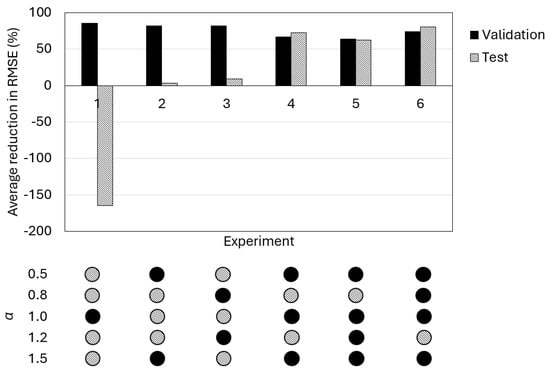
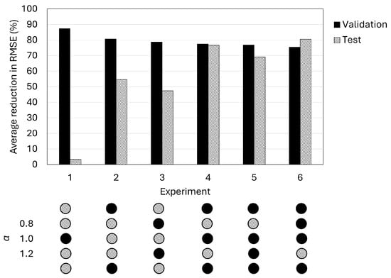
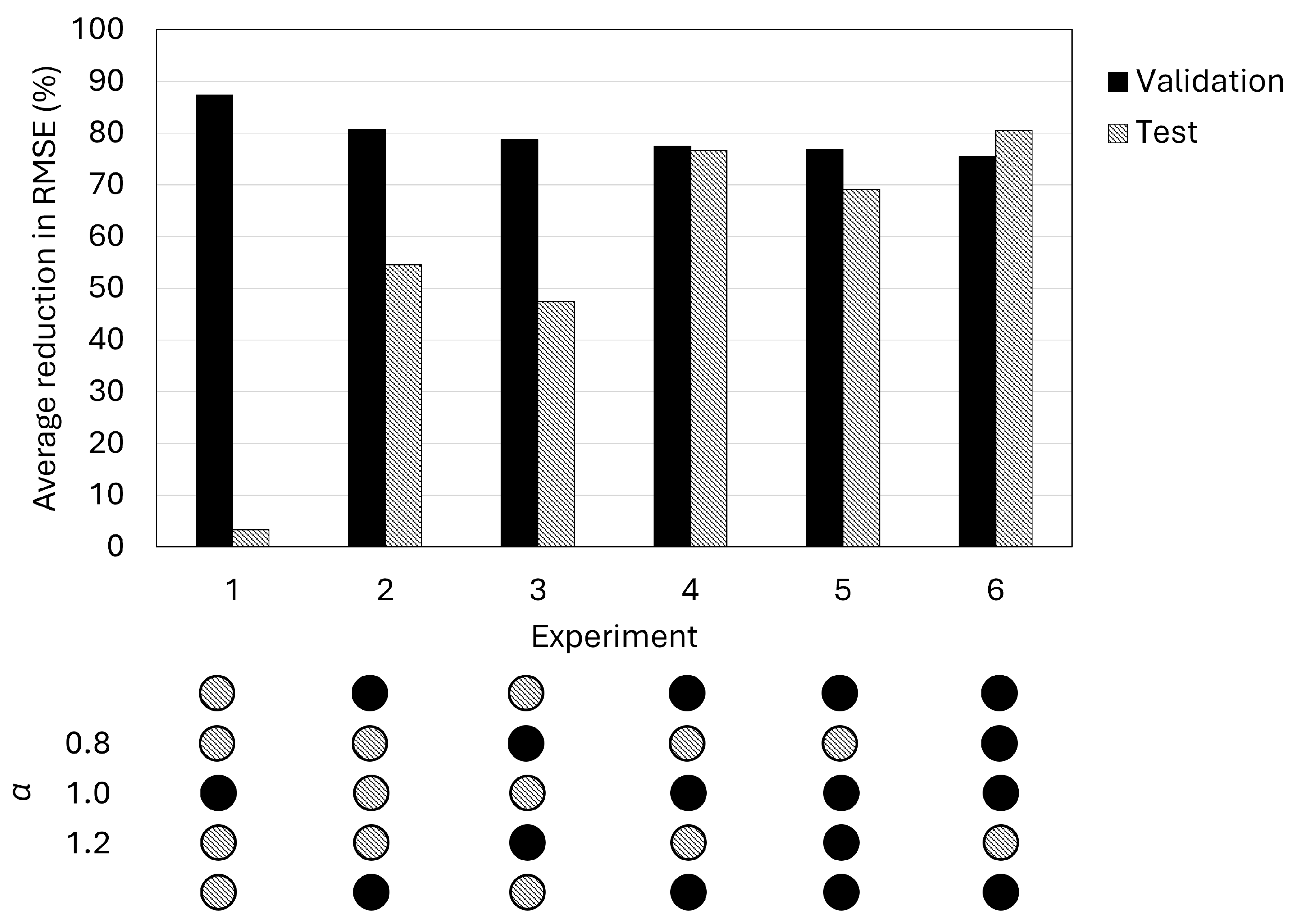
The same analysis was performed on the results from Experiments 1–6, comparing the RMSE in the seen and unseen geometries for each experiment, both for the two-branch and single-branch architecture. The results are shown in Figure 4 and Figure 5, respectively.
Figure 4.
Comparison of average RMSE reduction between the seen and unseen test sets for each experiment with the two-branch architecture. The combinations of included in each experiment are as shown. All experiments lead to a decrease in RMSE in the geometries seen in training. Only the experiments involving interpolation solely and having good coverage of the parameter space (Experiments 4–6) lead to a substantial decrease (>60%) in RMSE compared to RANS.
Figure 5.
Comparison of average RMSE reduction between the seen and unseen test sets for each experiment with the single-branch architecture. The combinations of included in each experiment are as shown. All experiments lead to a decrease in RMSE in the geometries seen in training. Only the experiments involving interpolation solely and having good coverage of the parameter space (Experiments 4–6) lead to a substantial decrease (>69%) in RMSE compared to RANS.
For the two-branch approach, a minimum of a 63% average reduction in the RMSE in the seen-geometry set is observed. Experiment 1 results in a worsening in RMSE for the unseen test geometries, indicating that having a single geometry in training is insufficient for generalisation. Experiments 2–3 result in a small improvement in RMSE as compared to RANS for the test geometries. Experiments 4–6 show the best generalisation to the test geometries, with at least a 60% improvement in the average RMSE.
For the single-branch approach, a minimum of a 75% average reduction in the RMSE in the seen-geometry set is observed. Across all six experiments, the model results in a positive improvement in the unseen test set. While the RMSE reduction in the test set in experiment 1 is not substantial, a more substantial improvement is observed in the other experiments. In Experiments 2–3, where two geometries are used for training, the reduction in RMSE is 50%. In Experiments 4–6, where three or more geometries are included in training, the biggest reduction in RMSE is observed (>69%).
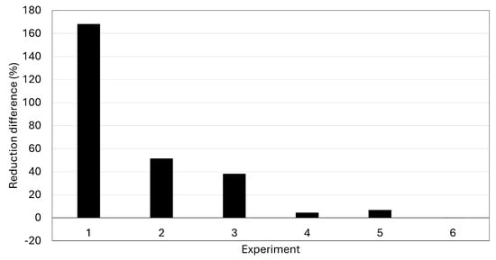
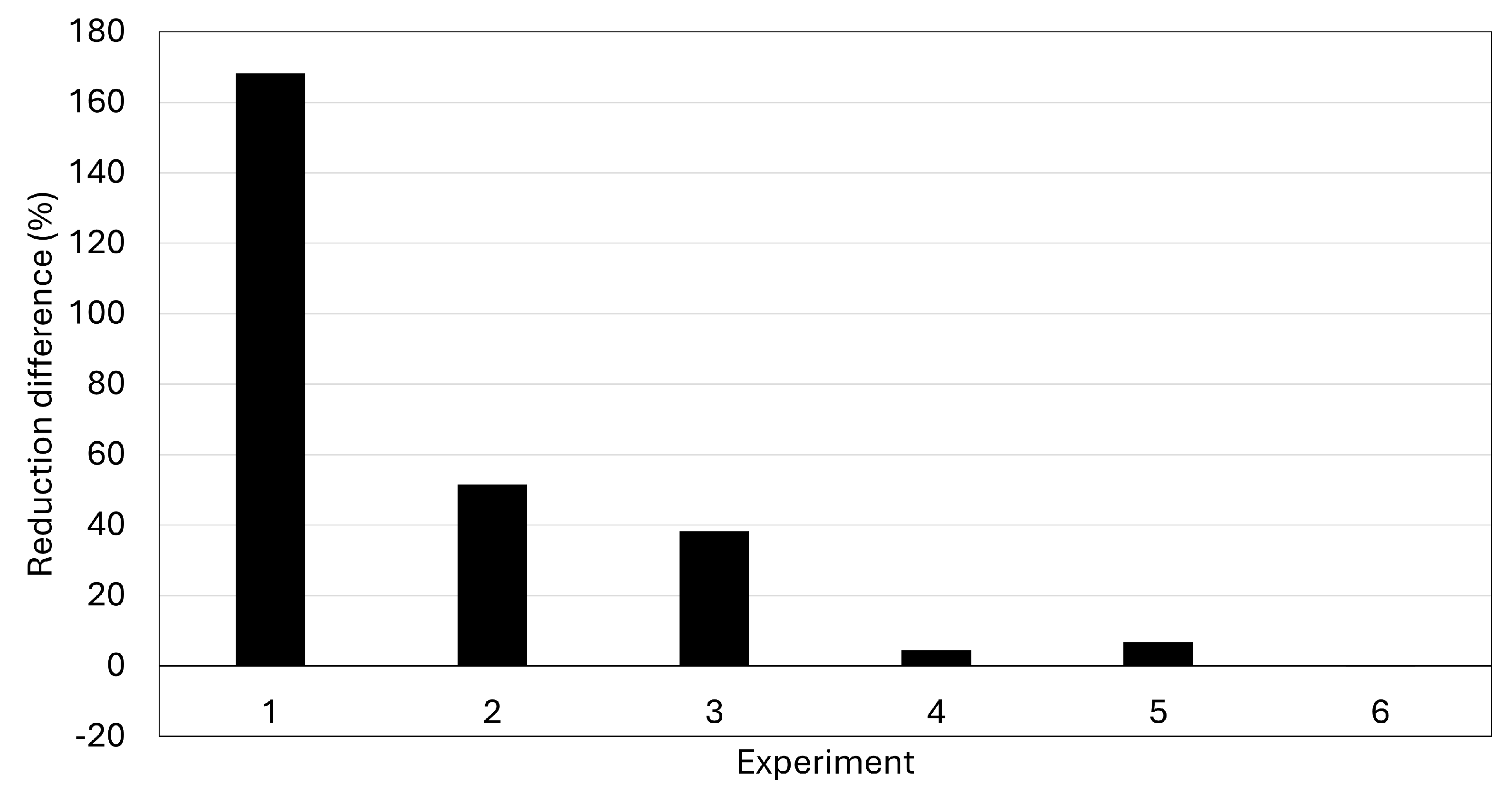
As the aim of this method is generalisation to unseen geometries, the most important metric to consider is the improvement of RMSE in the unseen test domain. Visual comparison of Figure 4 and Figure 5 shows that the single-branch method results in better generalisation. Figure 6 shows the difference between the reduction in RMSE in the unseen test set for the single-branch and the two-branch architecture. This shows that the single-branch architecture does the same or better that the two-branch architecture at generalising in the unseen test set. The biggest difference is observed in Experiments 1–3, which involve using fewer training cases. This shows that the additional complexity of the extra linear branch is not required for multi-fidelity learning in this application. The remaining analysis in this paper is therefore focused on the single-branch multi-fidelity neural network.
Figure 6.
Plots showing difference between RMSE reduction with the single-branch and the RMSE reduction with two-branch multi-fidelity neural network.
3.2. Generalisation Analysis
The generalisation capability of the single branch model is assessed across a range of training–testing configurations within the periodic hills parameter space. In this context, generalisation refers to the ability of the model to make accurate flow field predictions on the unseen-geometry test set.
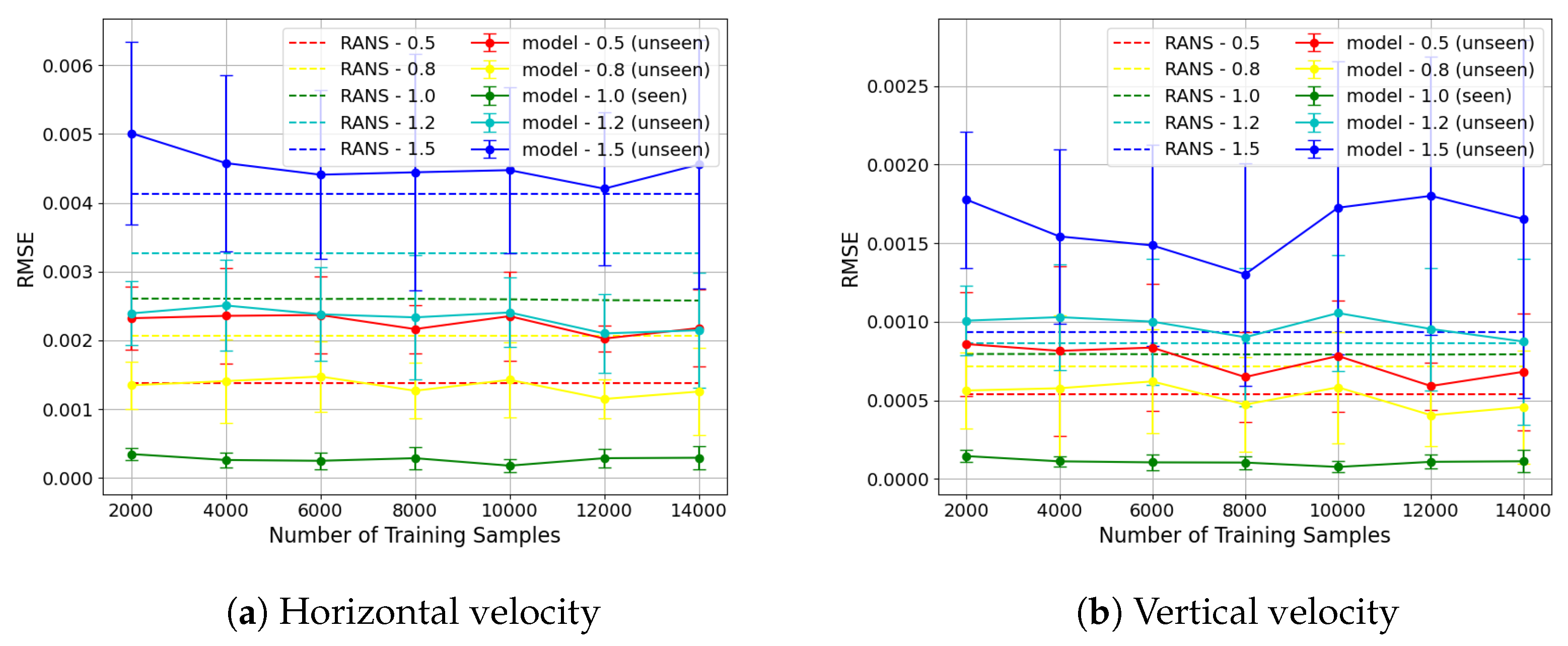
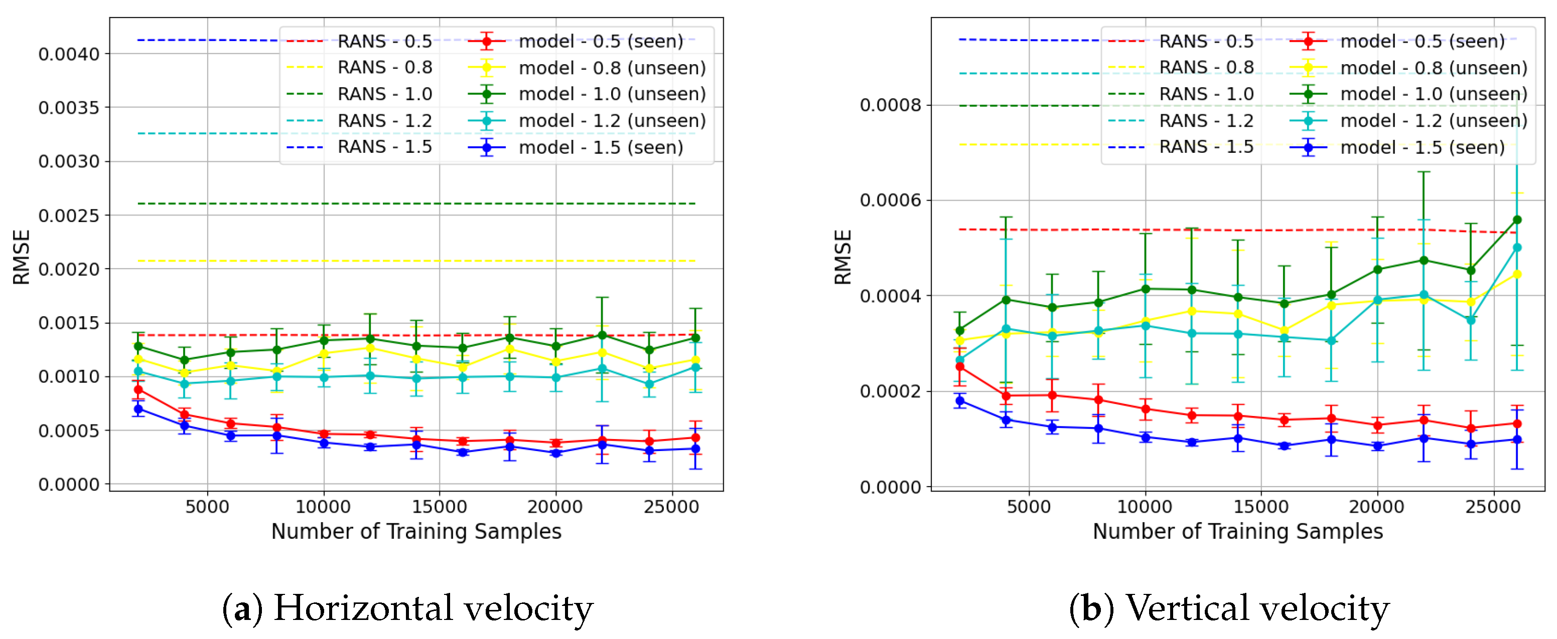
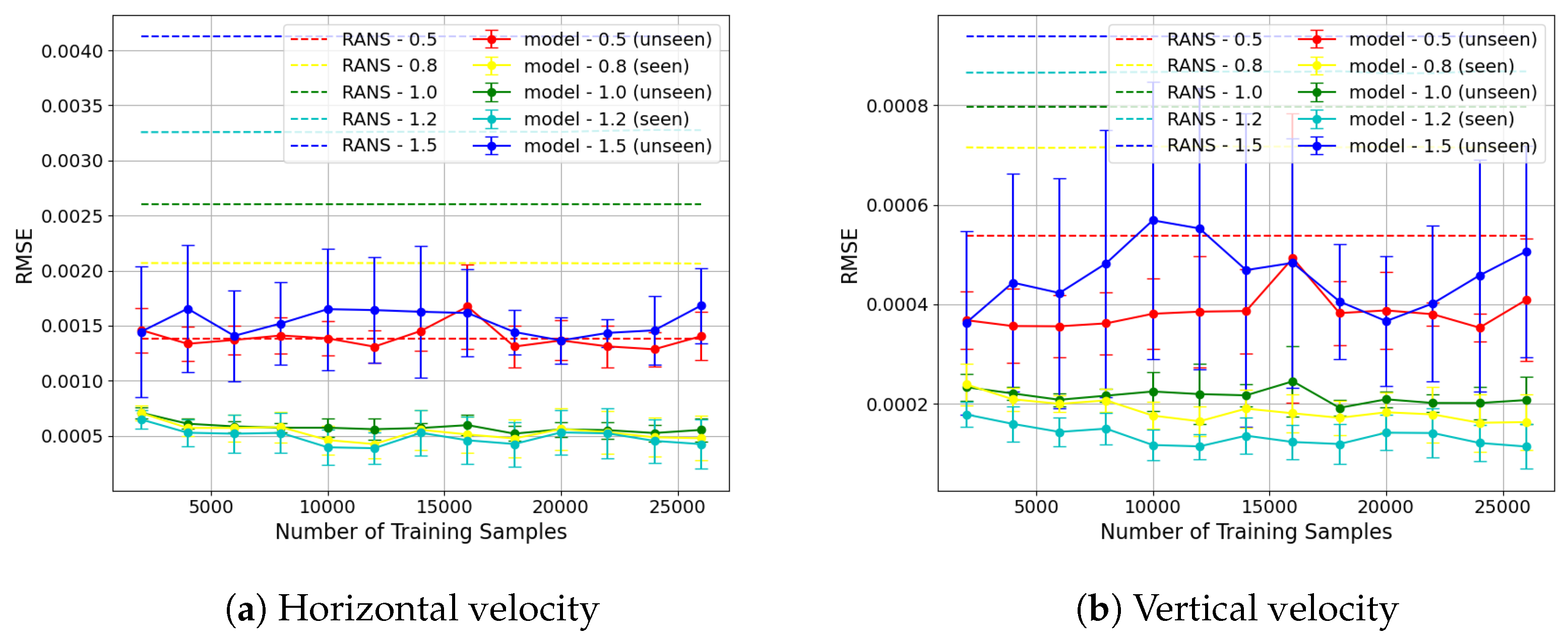
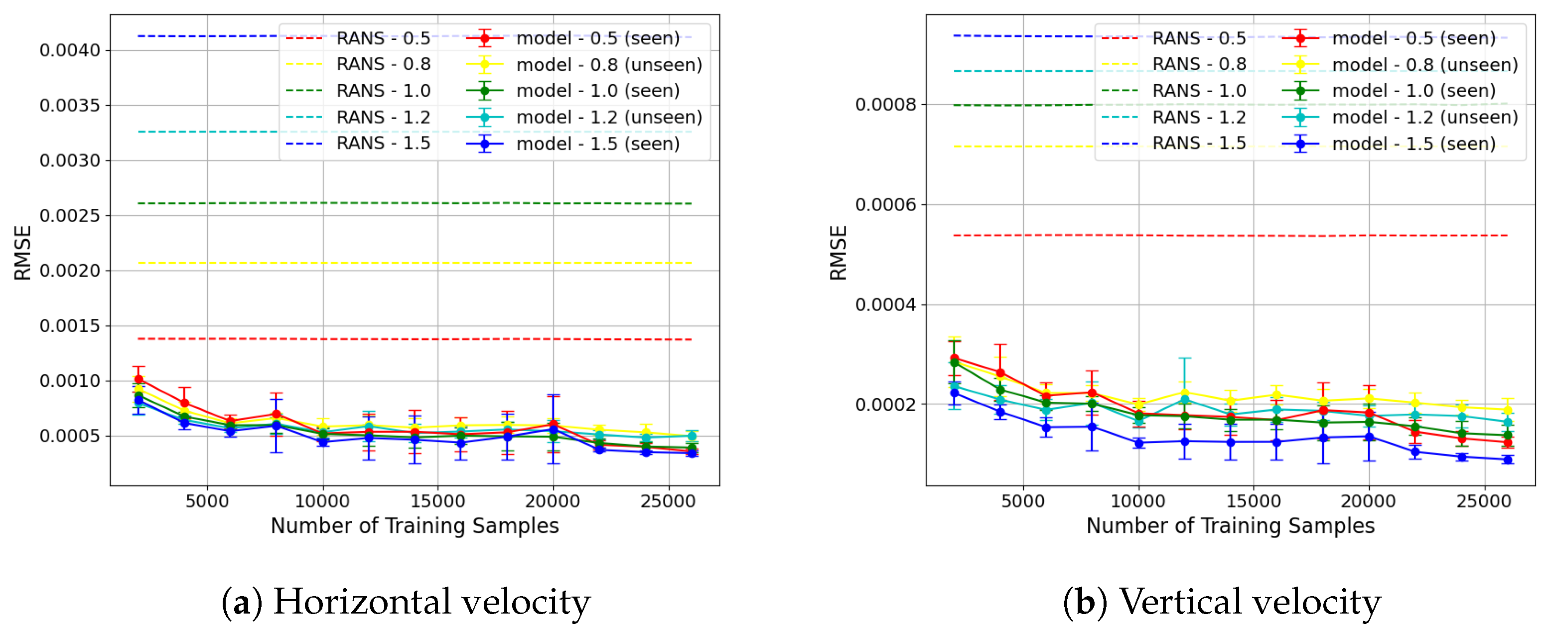
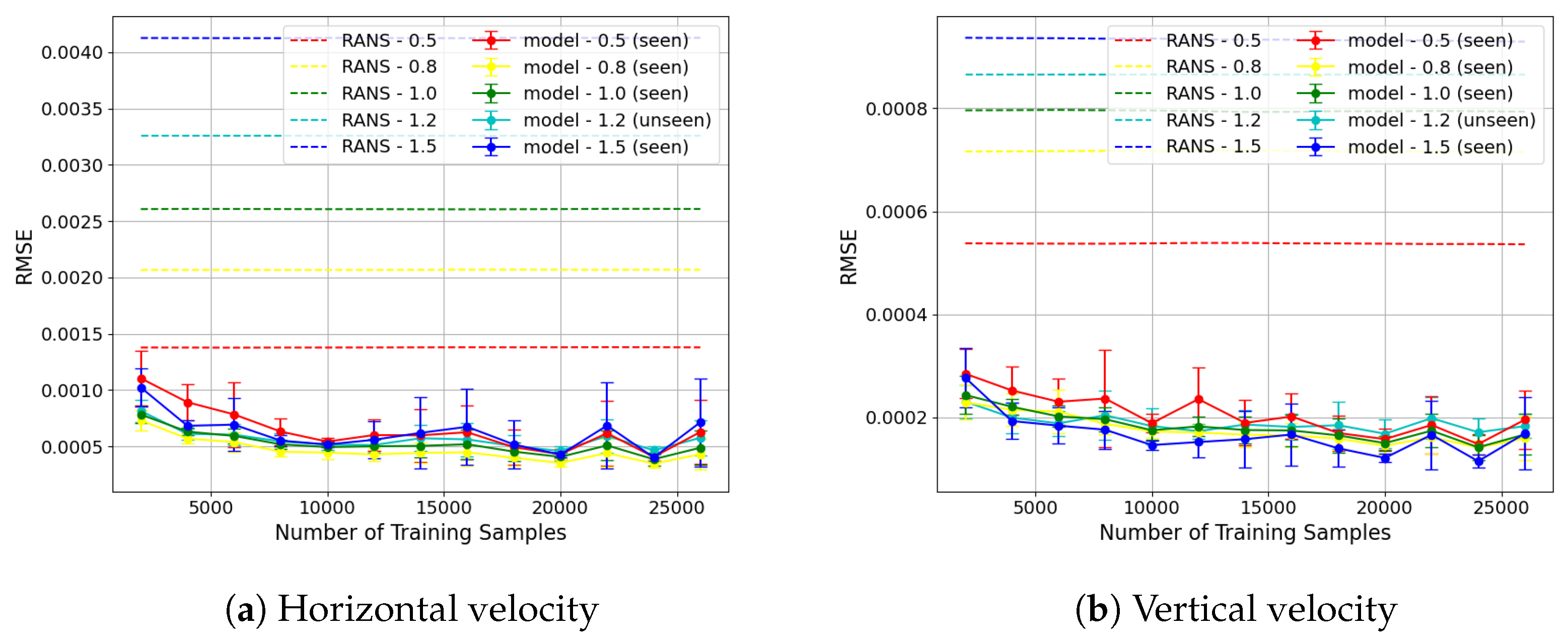
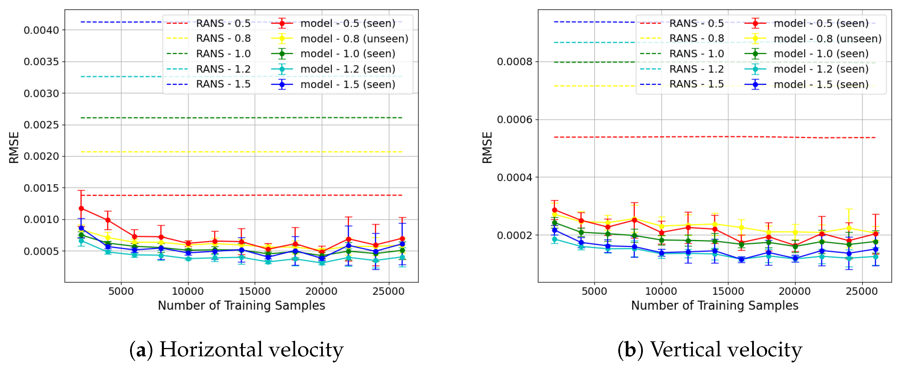
The results of the generalisation experiments are displayed in Figure 7, Figure 8, Figure 9, Figure 10, Figure 11 and Figure 12 as plots of RMSE versus number of training samples. The mean and standard deviation of the RMSE for each case are shown. For seen geometries, the RMSE was calculated on the held-out seen-geometry test set, whereas for the unseen test geometries, the RMSE was calculated over the whole domain. The RANS baseline RMSE (error between RANS and DNS) is also displayed. A detailed analysis of the results from each experiment is presented in Section 3.2.1, Section 3.2.2, Section 3.2.3, Section 3.2.4 and Section 3.2.5.
Figure 7.
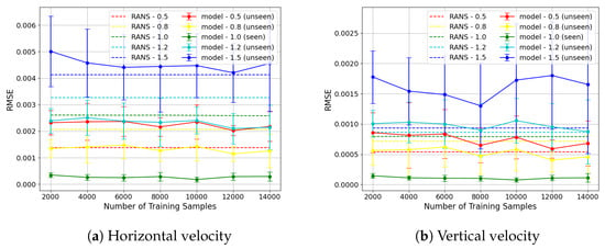
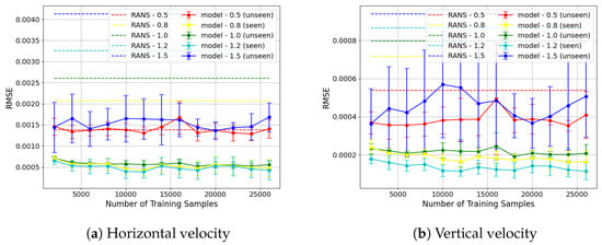
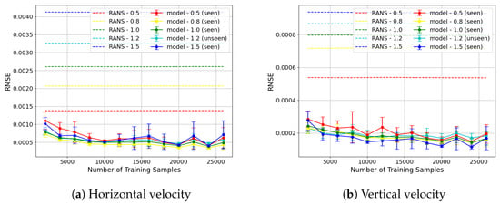
Plots showing RMSE (mean and standard deviation) across the seen-geometry test set ( = 1.0) and unseen-geometry test set ( = 0.5, 0.8, 1.2, 1.5) for each velocity component with different numbers of training samples from the seen geometries. The RMSE of the model prediction for the seen geometry ( = 1.0) is less than the RANS baseline. For close to the training case ( = 0.8, 1.2), limited generalisation to unseen geometries can be observed. For the other unseen geometries ( = 0.5, 1.5), the RMSE of the model prediction does not show an improvement from the RANS baseline, indicating poor generalisation.
Figure 8.
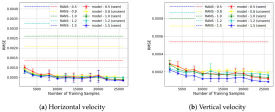
Plots showing RMSE (mean and standard deviation) across the seen-geometry test set ( = 0.5, 1.5) and unseen-geometry test set ( = 0.8, 1.0, 1.2) for each velocity component, with increasing numbers of training samples from the seen geometries. The RMSE in the seen-geometry test set is less than the RANS baselines for all number of samples, and shows a decreasing trend with number of samples. The unseen set also results in RMSE less than the RANS baseline.
Figure 9.
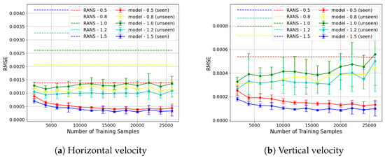
Plots showing RMSE across the seen-geometry test set ( = 0.8, 1.2) and unseen-geometry test set ( =0.5, 1.0, 1.5) for each velocity component, with increasing numbers of training samples from the seen geometries. The model improves the model prediction across all numbers of training samples for the seen geometries ( = 0.8, 1.2) and the middle unseen geometry, where = 1.0. The generalisation to the unseen edge cases, = 0.5, 1.5, is worse than the intermediate case of = 1.0.
Figure 10.
Plots showing RMSE across the seen-geometry test set ( = 0.5, 1.0, 1.5) and unseen geometries ( = 0.8, 1.2) for each velocity component, with increasing numbers of training samples from the seen geometries. The RMSE decreases with number of samples for both the seen and unseen cases.
Figure 11.
Plots showing RMSE across the seen-geometry test set ( = 0.5, 0.8, 1.0, 1.5) and unseen-geometry test set ( = 1.2) for each velocity component, with increasing numbers of training samples from the seen geometries. From N = 14,000, the model shows good reduction in RMSE as compared to RANS for both seen and unseen geometries.
Figure 12.
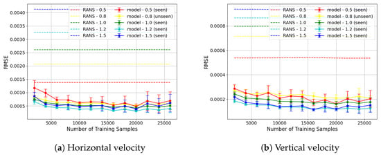
Plots showing RMSE across the seen-geometry test set ( = 0.5, 1.0, 1.2, 1.5) and unseen-geometry test set ( = 0.8) for each velocity component, with increasing numbers of training samples from the seen geometries. The model leads to substantial improvement in RMSE for the unseen geometry ( = 0.8). However, the prediction on the seen geometry, where = 0.5, shows no improvement or even a worsening in RMSE in multiple cases for the horizontal velocity.
Across the experiments, the generalisation performance of the model depends strongly on the coverage of the parameter space provided during training. Limited training configurations result in poor extrapolation, whereas increasing the diversity of training geometries enables accurate predictions on unseen geometries.
3.2.1. Experiment 1: Train = 1.0, Test = 0.5, 0.8, 1.2, 1.5
The results from Experiment 1 are shown in Figure 7. A lower RMSE is observed with the model prediction compared to the RMSE of the RANS baseline for both horizontal and vertical velocity components for the seen-geometry ( = 1.0) test set. For the horizontal velocity, the RMSE of the model prediction in the unseen geometries closest to the training case, = 0.8 and 1.2, is less than the corresponding RMSE in the RANS baseline. For the vertical velocity component, the RMSE of the prediction for = 0.8 is less than the corresponding RANS baseline whereas the RMSE of the prediction for = 1.2 is greater than the corresponding RANS baseline. The poorest performance is observed for = 0.5 and 1.5, which lie furthest from the training sample in terms of . The large mean errors and variance in this case highlight the difficulty of extrapolation from a single training geometry. These results demonstrate that training on a single geometry is insufficient to capture the variability across the parameter space, and emphasise the need for representative training coverage to enable generalisation.
3.2.2. Experiment 2: Train = 0.5, 1.5, Test = 0.8, 1.0, 1.2
In this experiment, the model was trained on two geometries ( = 0.5 and 1.5) and tested on three unseen geometries ( = 0.8, 1.0, 1.2). This setup evaluates interpolation capability across the parameterisation space. The results (Figure 8) show consistent improvement over the RANS baseline in the seen-geometry test sets. For unseen geometries, the model achieves improved performance across all unseen values. This shows that the model can generalise to unseen geometries with values between the values included in training. A negative correlation is observed between the error on the seen-geometry test set and the error on the unseen-geometry test set as the number of samples increases. This behaviour indicates that the model becomes increasingly specialised to the geometries included in the training set when more samples from those geometries are provided, without sufficient diversity in the geometries themselves. However, this behaviour is due to a distribution shift between the training/validation sets and the test set from the unseen geometries, as opposed to classical overfitting to training samples. As can be seen in the loss curves attached in the supplementary material, the training and validation losses, computed on the training geometries, converge without signs of overfitting. As the model becomes increasingly specialised to the geometries present in training, its ability to generalise to unseen geometries deteriorates. This indicates that in this situation, it would be preferable to use a model trained on fewer samples.
3.2.3. Experiment 3: Train = 0.8, 1.2, Test = 0.5, 1.0, 1.5
This experiment further evaluates interpolation and extrapolation by training on interior geometries ( = 0.8, 1.2). As shown in Figure 9, the model achieves strong performance on the seen-geometry test set and generalises effectively to the intermediate case = 1.0, where both RMSE and variance are low.
In contrast, performance degrades for the extrapolated edge cases ( = 0.5 and 1.5), with higher RMSE and variability. This behaviour highlights the greater challenge of extrapolation compared to interpolation, as is expected when applying data-driven models outside the training distribution.
3.2.4. Experiment 4: Train = 0.5, 1.0, 1.5, Test = 0.8, 1.2
In this experiment, training data was provided across the parameter space, including both edge and central geometries. The results (Figure 10) show a substantial improvement in generalisation performance compared to previous experiments.
For all N values, the model achieved lower RMSE than the RANS baseline for both seen and unseen geometries. Furthermore, the predictions exhibit reduced variance. Notably, even at low sample counts (), the model produced more accurate predictions than the baseline on unseen geometries.
These results demonstrate that providing sufficient coverage of the parameter space enables consistent and accurate generalisation.
Figures S1 and S2 in the Supplementary Materials show some examples of the loss curve from this experiment.
3.2.5. Experiments 5 and 6: Train on Data from 4 Different and Test on Remaining Case
In the final set of experiments, the model is trained on four geometries and tested on a single unseen case. The results (Figure 11 and Figure 12) show strong generalisation performance, with RMSE consistently below the RANS baseline.
Compared to Experiment 4, the inclusion of an additional training geometry provides only marginal improvements, indicating diminishing returns once sufficient parameter space coverage is achieved. The model maintains strong performance even with relatively small training datasets.
3.3. Flow Fields
In this section, examples of flow fields obtained on test geometries from Experiments 1 and 4 are displayed to compare flow characteristics observed when the model generalises well as opposed to when it does not. and are the non-dimensional horizontal and vertical velocities, respectively, normalised by the bulk velocity . It can be noted that the colour bars used for the flow fields (Figure 13, Figure 14, Figure 15, Figure 16, Figure 17 and Figure 18) differ between each figure, based on the individual minimum and maximum values.
Figure 13.
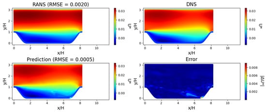
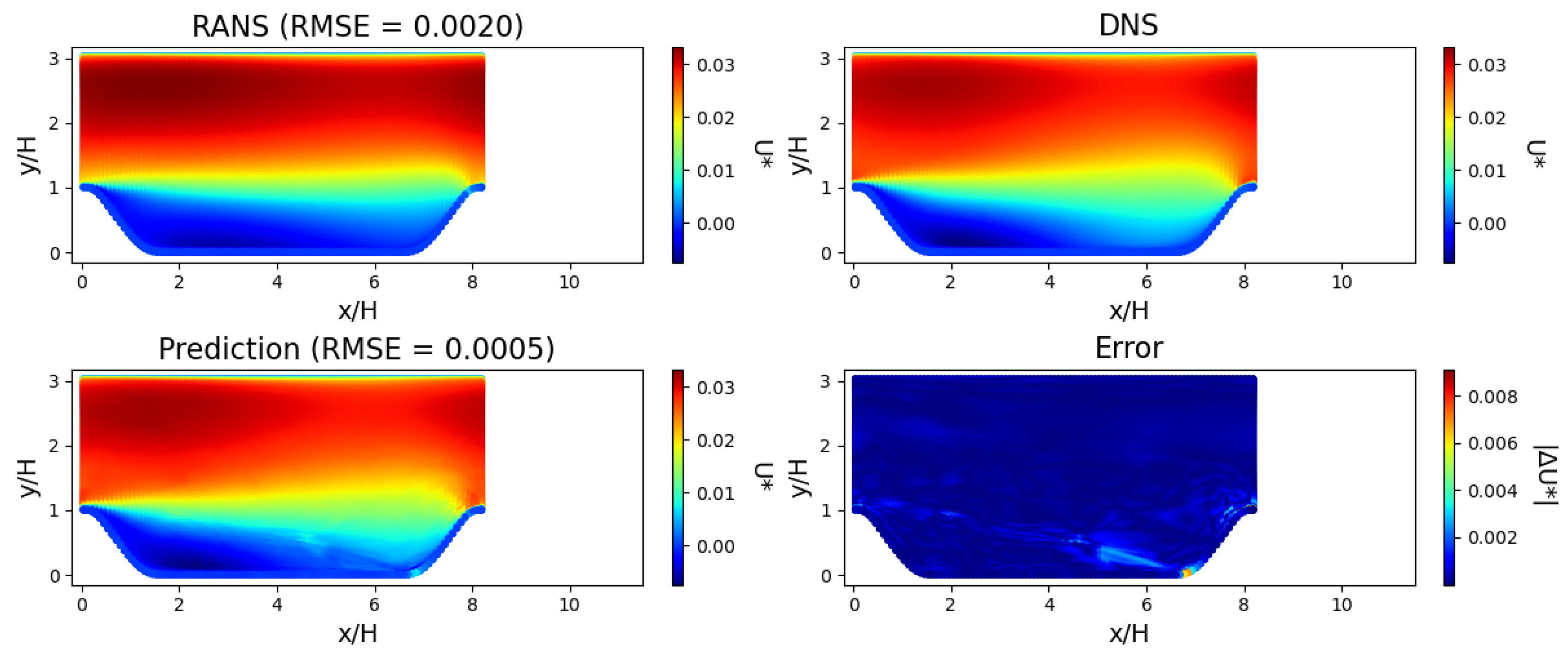
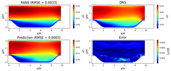
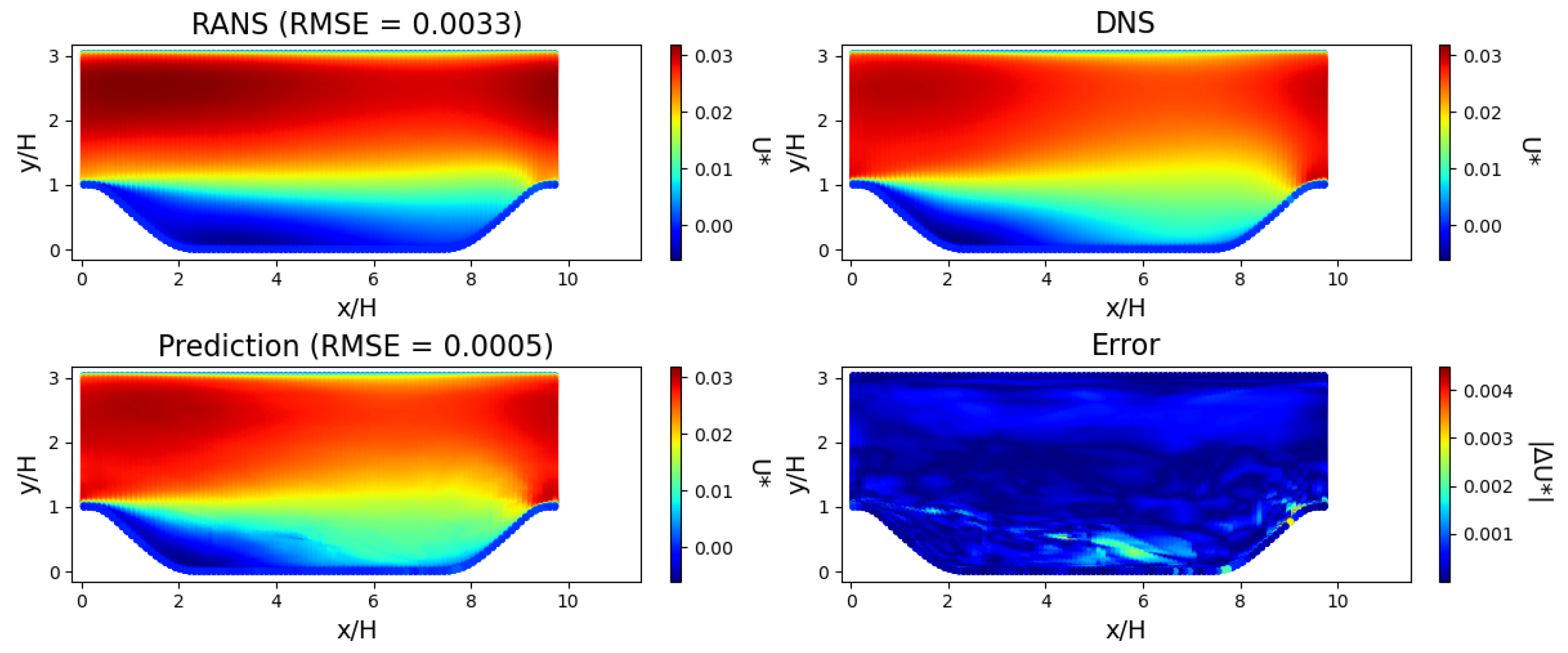
Horizontal flow field through periodic hill with = 0.8 for RANS, DNS, model prediction, and error between model prediction and DNS. The model was trained on data from = 0.5, 1.0 and 1.5. The RZL obtained from RANS is 5.6 and from DNS is 3.7. The RZL from the model prediction is 3.7, a match to the DNS value. The errors are concentrated close to the separation between the recirculation zone and the jet.
Figure 14.
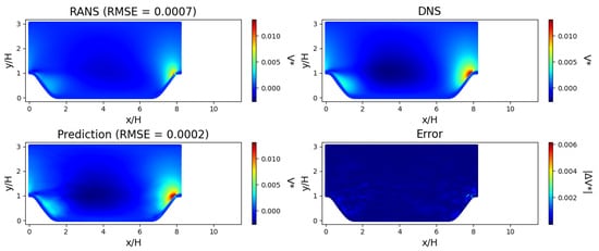
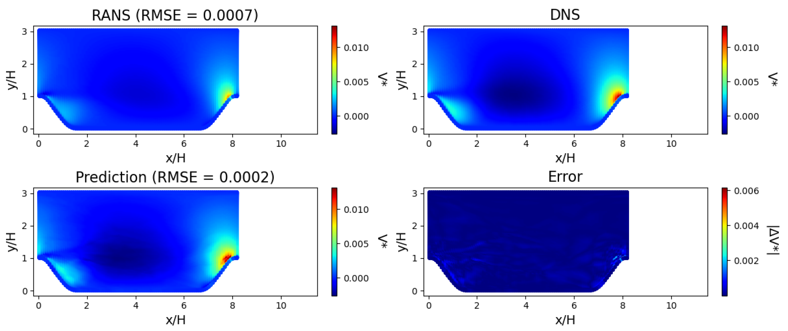
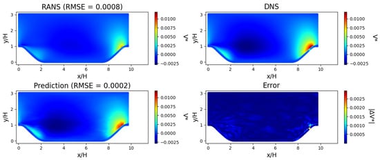
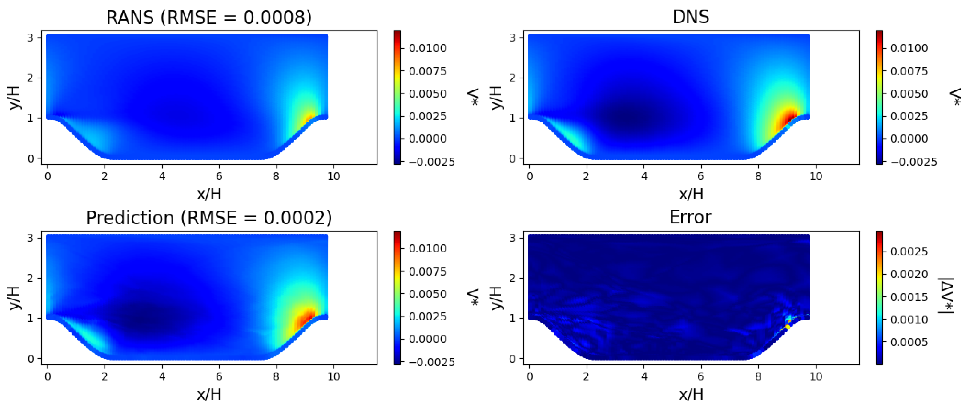
Vertical flow field through periodic hill with = 0.8 for RANS, DNS and model prediction, and error between model prediction and DNS. The model was trained on data from = 0.5, 1.0 and 1.5. The high velocity jet impinging onto the slope at the outlet gives rise to a high vertical velocity region. The size of this high velocity region is corrected by the model, resulting in a closer match to the DNS field than RANS.
Figure 15.
Horizontal flow field through periodic hill with = 1.2 for RANS, DNS and model prediction, and error between model prediction and DNS. The model was trained on data from domain of = 0.5, 1.0 and 1.5. The RZL obtained from RANS is 5.8 and from DNS is 3.5. The RZL from the model prediction is 3.5, which matches the DNS value. The errors are concentrated in the region of separation and close to the lower wall.
Figure 16.
Vertical flow field through periodic hill with = 1.2 for RANS, DNS and model prediction, and error between model prediction and DNS. The model was trained on data from domain of = 0.5, 1.0 and 1.5. The high velocity jet impinging onto the slope at the outlet gives rise to a high vertical velocity region. The size of this high velocity region is corrected by the model, resulting in a closer match to the DNS field than RANS.
Figure 17.
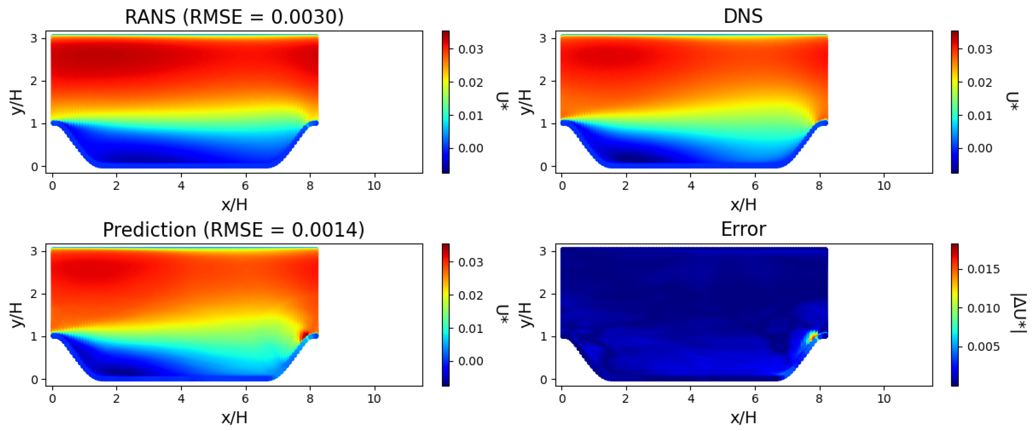
Horizontal flow field through periodic hill with = 0.8 for RANS, DNS, model prediction, and error between model prediction and DNS. The model was trained on data from domain of = 1.0. The RZL obtained from RANS is 5.6 and from DNS is 3.7. The RZL from the model prediction is 3.4, a closer match to the DNS value than the corresponding RANS value. The errors are concentrated around the region where the jet impinges onto the wall.
Figure 18.
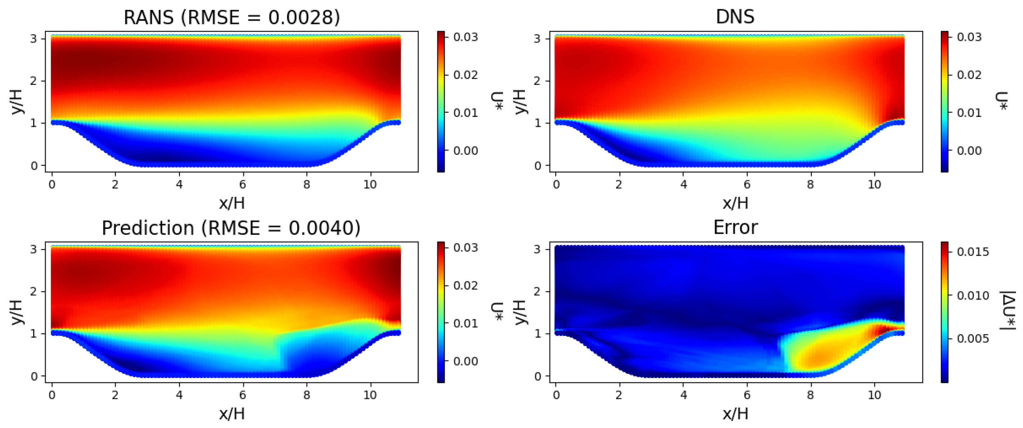
Horizontal flow field through periodic hill with = 1.5 for RANS, DNS, model prediction, and error between model prediction and DNS. The model was trained on data from domain of = 1.0. The predicted flow field does not show good agreement with the DNS, with high errors around the later part of the jet. The RMSE of the prediction is higher than the RMSE of the RANS solution.
Figure 13, Figure 14, Figure 15 and Figure 16 show the velocity flow field predictions from Experiment 4 on the test periodic hills ( = 0.8 and 1.2) for a model trained on data from = 0.5, 1.0 and 1.5. The model was trained on a total of 26,000 random points across the three geometries, with a uniform split between them. This experiment can be considered an interpolation case, as the seen training geometries are the edge and middle cases, and the unseen test geometries fall between these training cases.
From Figure 13, Figure 14, Figure 15 and Figure 16, the flow characteristics between RANS and time-averaged DNS can be compared. Similar features can be observed from both methods, with key differences being the length of the recirculation zone and the width of the jet formed from the separation:
- RANS overestimates the recirculation zone length (RZL) as compared to DNS. The RZL values are shown in Table 3.
- The width of the jet formed from the separation at the step is smaller with RANS than DNS.
Table 3.
Recirculation zone length (RZL) comparison between RANS and DNS for all values. RZL has been normalised with respect to step height.
From Figure 13, Figure 14, Figure 15 and Figure 16, it can be seen that the model successfully corrects the previously identified areas of inaccuracies: both the size and location of the recirculation zone and of the jet from the model prediction match the DNS results more closely than RANS. An example of this is shown in Figure 13, where the RZL for = 0.8 from the model prediction is 3.7, which is a substantial improvement considering the RZL from RANS and DNS are 5.6 and 3.7, respectively. This demonstrates the effectiveness of this method in improving the quality of RANS data, when provided with few examples of DNS data within the parameterised domain.
Experiment 1 involved training the model on the middle cases, i.e., training on data from = 1.0 and making a prediction on the remaining cases. The results of this experiment are shown in Figure 17 and Figure 18. For simplicity, only the horizontal velocity field for = 0.8 and 1.5 are shown. The predicted flow fields show that the model can generalise to the case of = 0.8, with the predicted flow fields showing a good match to the DNS data and a reduction in RMSE from RANS, as seen in Figure 17. However, the model does not generalise well to = 1.5, which is the most different from the training set both in terms of and the physical domain seen in training. As can be seen in Figure 18, the prediction results in large errors in the region of the jet impinging onto the wall, and the overall prediction RMSE is higher than the RANS RMSE.
3.4. Summary of Results
Overall, the results indicate that the model is capable of generalising effectively across unseen geometries within the considered parametric family. While extrapolation from limited training data leads to reduced accuracy as compared to interpolation, systematically increasing the diversity of the training set enables accurate predictions.
This progression highlights that generalisation is primarily governed by the coverage of the parameter space rather than sample size, and demonstrates that strong generalisation can be achieved within a controlled parametric regime.
4. Discussion
The comparison between the two-branch and single-branch multi-fidelity architectures shows that the additional linear branch does not improve generalisation performance for this application. As demonstrated in Section 3.1, the single-branch model consistently achieves equal or greater reductions in RMSE on unseen geometries across all experiments. This is even more noticeable in cases of low coverage of the parameter space (Experiments 1–3), indicating that the simpler architecture is better suited to learning the nonlinear relationship between RANS and DNS fields without requiring an explicit linear correction.
Overall, the results of this study show that multi-fidelity neural networks can provide substantial improvements over baseline RANS predictions for reconstructing velocity fields, even when trained on a limited number of geometries. A key aspect of this work is the comparison between interpolation and extrapolation using a small dataset. The model performs particularly well in interpolation cases, where the training data span the range of the parameter . The results show that when the training geometries cover the parameter space (Experiments 4–6), the model achieves reductions of at least 69% and 60% in RMSE compared to the RANS baseline on unseen cases, with the single-branch and two-branch architectures, respectively. This indicates that the model captures relationships between RANS and DNS fields. This behaviour is observed more clearly in the single-branch architecture, which maintains a positive RMSE reduction even in extrapolation cases where the two-branch model shows little or no improvement over the RANS baseline, as seen in Figure 6.
An important outcome of this study is that architectural complexity is not a prerequisite for effective multi-fidelity learning in this problem. The single-branch model, despite its simpler structure and smaller size, outperforms the two-branch model in generalisation to unseen geometries across all experiments. This suggests that the relationship between RANS and DNS fields is sufficiently captured by a single nonlinear mapping, and that additional linear correction pathways may introduce additional errors when training data is limited.
The sequence of experiments highlights the importance of how the training data are distributed. Adding more samples to a small number of geometries does not lead to the same improvement as adding geometries that fill gaps in the parameter space. For example, introducing in Experiment 4 leads to a clear improvement compared to Experiment 2, even though the total number of samples is similar. This shows that coverage of the parameter space has a stronger influence on performance than sample count alone. This coverage includes the parameter defining the slope of the the periodic hill, but also the physical space occupied by the whole domain. The extrapolation failures observed in Experiments 1–3 appear to arise from a coordinate-domain shift. As the model relies on spatial coordinates and RANS velocities as inputs, test geometries with physical domains that differ substantially from those seen in training (for example testing on = 1.5 when training on = 1.0) introduce regions of the domain that the network has not encountered. In contrast, cases where the physical domains overlap well (for example training on = 0.5 and 1.5) result in successful interpolation across intermediate geometries.
Another contribution of this work is the reconstruction of full velocity fields using DNS as the high-fidelity reference. Previous multi-fidelity studies have mainly focused on global quantities such as lift and drag [20,21,22]. In contrast, predicting full fields requires resolving local features such as separation and recirculation. The results show that substantial improvements over RANS can still be achieved in these cases when the model is applied within the training range.
The approach also avoids the use of explicit geometric parameters. Instead, the geometry is represented through spatial coordinates and flow variables. As the RANS solution reflects the underlying geometry, information on the geometry is already implicitly encoded in the spatial coordinates and velocity fields, allowing the model to learn geometry-dependent behaviour without an explicit parameter. This removes the need for a predefined geometric parameterisation and allows the same framework to be applied to different configurations, provided that similar conditions are included in the training data. The model uses coordinate-based inputs and does not require structured grid representations or image-based preprocessing. This makes it straightforward to apply once low and high-fidelity data are available on a common mesh. In practical terms, the method is suited to problems where low-fidelity simulations are readily available and a limited number of high-fidelity cases can be used to improve predictions. Although DNS is used in this study, the same approach can be applied to combinations such as RANS–LES. The model can therefore be used as a post-processing step to improve low-fidelity results.
5. Limitations and Future Work
While the method shows good generalisation to unseen geometries, several limitations remain. Firstly, the hyperparameter tuning carried out in this study was performed for the two-branch architecture and subsequently modified by removing the linear branch to give the single-branch model. Although the single-branch model still outperformed the two-branch model under these settings, it is possible that dedicated tuning could further improve its performance. Furthermore, the dataset used in this study contains only five geometries. While this allows a controlled comparison between interpolation and extrapolation, it limits the range of flow features available during training. Extending the dataset to include additional geometries would increase coverage of the parameter space and is expected to improve predictive performance on unseen cases. Higher errors are observed near walls and in separation regions. These areas involve strong gradients and are more difficult to predict accurately, as also noted in previous studies [24]. Improving predictions in these regions may require incorporating additional physical constraints or modifying the model architecture. While removing explicit geometric parameters simplifies the model, it means that geometric variation must be learned from the training data alone. For more varied or higher-dimensional geometries, this will require careful selection of training cases to ensure adequate representation of the domain. Future work will therefore focus on expanding the range of geometries and applying the method to more complex flows, including three-dimensional and practical engineering configurations.
6. Conclusions
In this study, it is demonstrated that multi-fidelity neural networks can produce substantial improvement in velocity flow fields obtained from RANS simulations in unseen geometries, when trained on a subset of higher fidelity DNS data. Multi-fidelity neural networks were applied to a curated dataset of parameterised periodic hills, and generalisation was evaluated across six training–testing configurations. The main contributions are: (1) a comparative analysis revealing that a single-branch multi-fidelity architecture consistently outperforms a two-branch alternative in this application; (2) a quantitative assessment showing that coverage of the parameter space is the primary driver of generalisation performance, resulting in large reductions in RMSE in unseen geometries when training geometries are well distributed.
Quantitatively, the strongest improvements were obtained by interpolation between well-spaced training geometries. When trained on three evenly distributed geometries, RMSE on unseen test geometries was reduced by at least 69% relative to the RANS baseline (mean reduction across velocity components and test cases) with the single-branch model. Across all experiments, equal or greater RMSE reductions were produced by the single-branch architecture compared with the two-branch model. The biggest difference was observed in experiments with low coverage of the parameter space (Experiments 1–3), where positive RMSE reduction was maintained by the single-branch model while the two-branch model showed little or no improvement. From these results, it was inferred that the dominant relationship between RANS and DNS fields in this parametric family can be captured effectively by a single nonlinear mapping, and that the addition of an explicit linear correction branch does not improve, and in some cases, may degrade generalisation.
This method has several practical advantages, including not requiring explicit geometric parameters and physical representations of the domain as model inputs. These properties reduce preprocessing overhead and broaden applicability to geometries that lack simple parameterisations. Furthermore, the model can help reconstruct complete velocity fields rather than only global quantities. Future work will include additional geometries to improve parameter space coverage and to assess whether the single-branch advantage persists with bigger training sets. The approach will also be extended to three dimensional and more complex engineering flows to evaluate generalisability of multi-fidelity flow reconstruction in practical CFD workflows.
Supplementary Materials
The following supporting information can be downloaded at https://www.mdpi.com/article/10.3390/fluids11090208/s1: Figure S1: Loss curve for model trained on = 0.5 and 1.5, and number of samples = 10,000; Figure S2: Loss curve for model trained on = 0.5 and 1.5, and number of samples = 26,000.
Author Contributions
H.G. Conceptualization, Methodology, Writing—Original Draft, A.P.B.: Writing—Review & Editing, Supervision. A.N.C.: Writing—Review & Editing, Supervision. K.H.F.: Conceptualization, Writing—Review & Editing, Funding acquisition, Supervision. All authors have read and agreed to the published version of the manuscript.
Funding
This work was supported by the UKRI Centre for Doctoral Training in Accountable, Responsible and Transparent AI (ART-AI) [EP/S023437/1] and the University of Bath.
Data Availability Statement
The dataset used in this study is an open-source dataset, curated for the development of machine learning methods for corrective turbulence modelling [28]. Data available here: https://www.kaggle.com/datasets/ryleymcconkey/ml-turbulence-dataset (accessed on 16 January 2025).
Acknowledgments
This research made use of Hex, the GPU Cloud in the Department of Computer Science at the University of Bath.
Conflicts of Interest
The authors declare no conflicts of interest.
References
- Reynolds, W.C. The potential and limitations of direct and large eddy simulations. In Whither Turbulence? Turbulence at the Crossroads; Springer: Berlin/Heidelberg, Germany, 1990; pp. 313–343. [Google Scholar]
- Dhert, T.; Ashuri, T.; Martins, J.R. Aerodynamic shape optimization of wind turbine blades using a Reynolds-averaged Navier–Stokes model and an adjoint method. Wind. Energy 2017, 20, 909–926. [Google Scholar] [CrossRef] [Scilit]
- Lien, F.S.; Yee, E. Numerical modelling of the turbulent flow developing within and over a 3-d building array, part I: A high-resolution Reynolds-averaged Navier—Stokes approach. Bound.-Layer Meteorol. 2004, 112, 427–466. [Google Scholar] [CrossRef] [Scilit]
- Nissim, L.; Karnik, S.; Smith, P.A.; Wang, Y.; Frazier, O.H.; Fraser, K.H. Machine learning based on computational fluid dynamics enables geometric design optimisation of the NeoVAD blades. Sci. Rep. 2023, 13, 7183. [Google Scholar] [CrossRef] [Scilit] [PubMed]
- Langtry, R.B.; Menter, F.R. Correlation-Based Transition Modeling for Unstructured Parallelized Computational Fluid Dynamics Codes. AIAA J. 2009, 47, 2894–2906. [Google Scholar] [CrossRef] [Scilit]
- Schultz, M.G.; Betancourt, C.; Gong, B.; Kleinert, F.; Langguth, M.; Leufen, L.H.; Mozaffari, A.; Stadtler, S. Can deep learning beat numerical weather prediction? Philos. Trans. R. Soc. A 2021, 379, 20200097. [Google Scholar] [CrossRef] [Scilit] [PubMed]
- Ti, Z.; Deng, X.W.; Yang, H. Wake modeling of wind turbines using machine learning. Appl. Energy 2020, 257, 114025. [Google Scholar] [CrossRef] [Scilit]
- Li, J.; Du, X.; Martins, J.R. Machine learning in aerodynamic shape optimization. Prog. Aerosp. Sci. 2022, 134, 100849. [Google Scholar] [CrossRef] [Scilit]
- Wang, H.; Cao, Y.; Huang, Z.; Liu, Y.; Hu, P.; Luo, X.; Song, Z.; Zhao, W.; Liu, J.; Sun, J.; et al. Recent advances on machine learning for computational fluid dynamics: A survey. arXiv 2024, arXiv:2408.12171. [Google Scholar]
- Ling, J.; Kurzawski, A.; Templeton, J. Reynolds averaged turbulence modelling using deep neural networks with embedded invariance. J. Fluid Mech. 2016, 807, 155–166. [Google Scholar] [CrossRef] [Scilit]
- Kaandorp, M.L.; Dwight, R.P. Data-driven modelling of the Reynolds stress tensor using random forests with invariance. Comput. Fluids 2020, 202, 104497. [Google Scholar] [CrossRef] [Scilit]
- Jiang, C.; Vinuesa, R.; Chen, R.; Mi, J.; Laima, S.; Li, H. An interpretable framework of data-driven turbulence modeling using deep neural networks. Phys. Fluids 2021, 33, 055133. [Google Scholar] [CrossRef] [Scilit]
- Gamahara, M.; Hattori, Y. Searching for turbulence models by artificial neural network. Phys. Rev. Fluids 2017, 2, 054604. [Google Scholar] [CrossRef] [Scilit]
- Li, H.; Zhao, Y.; Wang, J.; Sandberg, R.D. Data-driven model development for large-eddy simulation of turbulence using gene-expression programing. Phys. Fluids 2021, 33, 125127. [Google Scholar] [CrossRef] [Scilit]
- Beck, A.; Flad, D.; Munz, C.D. Deep neural networks for data-driven LES closure models. J. Comput. Phys. 2019, 398, 108910. [Google Scholar] [CrossRef] [Scilit]
- Sirignano, J.; MacArt, J.F.; Freund, J.B. DPM: A deep learning PDE augmentation method with application to large-eddy simulation. J. Comput. Phys. 2020, 423, 109811. [Google Scholar] [CrossRef] [Scilit]
- Brenner, O.; Plogmann, J.; Piroozmand, P.; Jenny, P. A variational data assimilation approach for sparse velocity reference data in coarse RANS simulations through a corrective forcing term. Comput. Methods Appl. Mech. Eng. 2024, 427, 117026. [Google Scholar] [CrossRef] [Scilit]
- Bidar, O.; Anderson, S.; Qin, N. Sensor placement for data assimilation of turbulence models using eigenspace perturbations. Phys. Fluids 2024, 36, 015144. [Google Scholar] [CrossRef] [Scilit]
- Plogmann, J.; Brenner, O.; Jenny, P. Variational assimilation of sparse time-averaged data for efficient adjoint-based optimization of unsteady RANS simulations. Comput. Methods Appl. Mech. Eng. 2024, 427, 117052. [Google Scholar] [CrossRef] [Scilit]
- He, L.; Qian, W.; Zhao, T.; Wang, Q. Multi-fidelity aerodynamic data fusion with a deep neural network modeling method. Entropy 2020, 22, 1022. [Google Scholar] [CrossRef] [Scilit] [PubMed]
- Zhang, X.; Xie, F.; Ji, T.; Zhu, Z.; Zheng, Y. Multi-fidelity deep neural network surrogate model for aerodynamic shape optimization. Comput. Methods Appl. Mech. Eng. 2021, 373, 113485. [Google Scholar] [CrossRef] [Scilit]
- Liao, P.; Song, W.; Du, P.; Zhao, H. Multi-fidelity convolutional neural network surrogate model for aerodynamic optimization based on transfer learning. Phys. Fluids 2021, 33, 127121. [Google Scholar] [CrossRef] [Scilit]
- Sánchez-Moreno, F.; MacManus, D.; Tejero, F.; Sheaf, C. Nacelle optimisation through multi-fidelity neural networks. Int. J. Numer. Methods Heat Fluid Flow 2024, 34, 3615–3634. [Google Scholar] [CrossRef] [Scilit]
- Li, J.; Li, Y.; Liu, T.; Zhang, D.; Xie, Y. Multi-fidelity graph neural network for flow field data fusion of turbomachinery. Energy 2023, 285, 129405. [Google Scholar] [CrossRef] [Scilit]
- Meng, X.; Karniadakis, G.E. A composite neural network that learns from multi-fidelity data: Application to function approximation and inverse PDE problems. J. Comput. Phys. 2020, 401, 109020. [Google Scholar] [CrossRef] [Scilit]
- Ribeiro, M.D.; Rehman, A.; Ahmed, S.; Dengel, A. DeepCFD: Efficient steady-state laminar flow approximation with deep convolutional neural networks. arXiv 2020, arXiv:2004.08826. [Google Scholar]
- Zhang, W.; Zhang, C.; Zhao, Y.; Wang, Z.; Liu, Y.; Zhou, C.; Hu, Y. Convolutional neural networks-based surrogate model for fast computational fluid dynamics simulations of indoor airflow distribution. Energy Build. 2025, 326, 115020. [Google Scholar] [CrossRef] [Scilit]
- McConkey, R.; Yee, E.; Lien, F.S. A curated dataset for data-driven turbulence modelling. Sci. Data 2021, 8, 255. [Google Scholar] [CrossRef] [Scilit] [PubMed]
- Breuer, M.; Peller, N.; Rapp, C.; Manhart, M. Flow over periodic hills–numerical and experimental study in a wide range of Reynolds numbers. Comput. Fluids 2009, 38, 433–457. [Google Scholar] [CrossRef] [Scilit]
- Rapp, C.; Manhart, M. Flow over periodic hills: An experimental study. Exp. Fluids 2011, 51, 247–269. [Google Scholar] [CrossRef] [Scilit]
- Bentaleb, Y.; Lardeau, S.; Leschziner, M.A. Large-eddy simulation of turbulent boundary layer separation from a rounded step. J. Turbul. 2012, 13, N4. [Google Scholar] [CrossRef] [Scilit]

Disclaimer/Publisher’s Note: The statements, opinions and data contained in all publications are solely those of the individual author(s) and contributor(s) and not of MDPI and/or the editor(s). MDPI and/or the editor(s) disclaim responsibility for any injury to people or property resulting from any ideas, methods, instructions or products referred to in the content. |
© 2026 by the authors. Licensee MDPI, Basel, Switzerland. This article is an open access article distributed under the terms and conditions of the Creative Commons Attribution (CC BY) license.