Numerical Investigation of Sweeping-Jet Control at the Nose Region of a High-Speed Train

Abstract

With the increase in operating speed, aerodynamic drag becomes a major part of the total resistance of high-speed trains. Further drag reduction by only optimizing the streamlined shape is difficult. In this study, a three-car high-speed train model was used to explore active drag reduction by sweeping jets. The improved delayed detached-eddy simulation (IDDES) method based on the SST k-ω turbulence model was adopted. An equivalent sweeping-jet model was used to reduce the computational cost. Three important parameters were considered: the outlet width of the sweeping-jet model, the jet angle, and the jet velocity. The results show that a larger jet outlet gives a stronger drag-reduction effect. When the ratio between the jet outlet width and the train width is 5:50, the total drag reduction in the three-car train reaches about 1.5%. When the jet angle is 120°, the total drag reduction reaches about 2.84%, and the middle car has the largest drag reduction of 6.19%. When the jet velocity is 0.30 times the incoming flow velocity, the total drag reduction reaches about 4.0%. The main flow-control mechanism is that the sweeping jet forms a low-speed recirculation region near the train surface. This region lifts the incoming flow, weakens its direct impact on the train body, and reduces the surface pressure in the controlled region. The results provide a useful basis for applying sweeping jets to aerodynamic drag reduction in high-speed trains.

1. Introduction

High-speed railway is an important part of modern transportation. It has high speed, large carrying capacity, good economic benefits, low pollution, and good passenger comfort. For this reason, high-speed railway plays an important role in national economic development [1,2,3].

As the train speed increases, aerodynamic drag increases rapidly and becomes the main source of running resistance. When the train speed is 120 km/h, aerodynamic drag is about 40% of the total resistance. When the speed is 200–300 km/h, this value increases to about 70–80%. When the speed is higher than 300 km/h, aerodynamic drag may exceed 85% of the total resistance [4,5,6]. Therefore, reducing aerodynamic drag is important for lowering energy consumption and improving the operating economy of high-speed trains.

Many researchers have optimized the streamlined shape of the head and tail cars to reduce drag [7,8,9]. Shape optimization can suppress flow separation around the train and reduce the aerodynamic force. Zhang [10] carried out wind-tunnel tests and found that a larger slenderness ratio for the head car can improve the drag-reduction effect. However, head-shape optimization has only a limited effect on the middle car, while the shape of the tail car has a strong influence on the drag of the tail car. Zhang and Zhou [11] tested four CRH2 head shapes with different slenderness ratios and found that a longer and smoother streamlined head with a sharper nose gives better aerodynamic performance. Chen and Zhai [12] studied different head shapes and showed that a single-arch head shape has better drag-reduction performance than a double-arch head shape. Muñoz-Paniagua and García [9] optimized the head shape using a genetic algorithm and reduced the drag coefficient by 32.5% compared with the reference model. Zhang et al. [13] optimized the head and tail streamlined regions separately and found that using different optimized shapes for the head and tail cars can give a much stronger drag-reduction effect than using the same shape.

However, when the streamlined length reaches a certain limit, the aerodynamic drag coefficient stabilizes, and the improvement from further shape optimization becomes marginal. Consequently, alternative drag-reduction strategies are required. Various active flow control (AFC) techniques have been extensively explored for aerodynamic drag reduction, including steady blowing and suction [14,15], synthetic jets [16,17], and pulsed jets [18]. Despite their aerodynamic benefits, these conventional AFC strategies encounter specific limitations in practical engineering applications. For instance, steady jets generally exhibit a restricted effective control range and low energy efficiency. Synthetic jet actuators often suffer from system complexity and poor mechanical robustness under rigorous operational conditions. Similarly, pulsed jets tend to provide inferior flow entrainment compared to spatially oscillating flows. To overcome these bottlenecks, the sweeping jet (SWJ)—generated by a fluidic oscillator—has emerged as a viable alternative. Characterized by a broad sweeping coverage and the complete absence of internal moving parts, SWJ oscillators offer improved flow entrainment capability, efficiency, and structural reliability, thereby presenting unique advantages for robust active flow control.

Khan et al. [19] used a single fluidic oscillator on an Ahmed-type transport model and showed that sweeping jets can reduce drag and suppress the wake RSB mode. Cerretelli and Kirtley [20] used sweeping jets to control boundary-layer separation in a diffuser and reported that sweeping jets can provide similar control performance with lower power and momentum input than a steady jet. Seifert et al. [21] studied active flow control on large trucks and showed that sweeping jets can reduce the drag of a full-scale truck by about 10%. Seele et al. [22] used bistable sweeping jets to delay separation on a V-22 wing model and obtained drag reduction and lift increase. Woszidlo et al. [23] improved the flow around a multi-element airfoil with sweeping jets and reduced the required momentum input. Chen et al. [24,25] studied sweeping jets on a slanted-base cylinder, which can be regarded as an equivalent model of a high-speed train tail car, and explained the mechanism of wake-vortex control and drag reduction.

Based on these studies, the present work applies sweeping jets to the key aerodynamic regions of a high-speed train. The effects of jet outlet size, jet angle, and jet velocity are investigated by numerical simulation. The purpose is to clarify the drag-reduction law and the flow-control mechanism of sweeping jets for high-speed trains.

2. Numerical Method and Model

2.1. Governing Equations and Numerical Method

The Improved Delayed Detached-Eddy Simulation (IDDES) is a hybrid computational model that combines the advantages of RANS and LES, employing RANS in near-wall regions and switching to LES in detached flow regions away from the wall. Traditional DES methods are prone to Modeled Stress Depletion (MSD) and grid-induced unphysical separation in the transition region due to insufficient grid resolution. IDDES overcomes these drawbacks by defining the subgrid length scale as a function of both grid size and wall distance. This improvement effectively prevents MSD and premature flow separation, making it suitable for simulating large-scale separated flows. Furthermore, incorporating the SST k-w turbulence model accurately addresses the transport of turbulent shear stress, significantly improving the prediction accuracy of adverse pressure gradients and pressure-induced separation.

An incompressible Navier–Stokes solver was used in this study. The SIMPLE algorithm was used for pressure–velocity coupling. To minimize numerical dissipation and accurately resolve the separated turbulent eddies within the IDDES framework, the spatial discretization for the convective terms of the momentum equations was achieved using the bounded central differencing (BCD) scheme. A second-order discretization scheme was adopted for the time term of the implicit unsteady model. To obtain stable time-averaged results, the total calculation time was set to 1.5 s. The Courant number (Cr) can be used to estimate a reasonable time step. The Courant number is defined as follows:

$$Cr={\displaystyle \frac{U\infty \times dt}{L}}$$

(1)

where U_∞ is the incoming flow velocity, dt represents the time step, and L is the minimum cell size. While ensuring the calculation accuracy, the Courant number is appropriately increased to improve the calculation efficiency. Finally, the time step was set to 5 × 10⁻⁵ s. Regarding the convergence criteria, the maximum number of inner iterations within each time step was set to 4. Due to the highly unsteady nature of the massive flow separation around the high-speed train, the equation residuals do not drop monotonically to machine zero. Instead, the computation was deemed converged when the continuity and momentum residuals exhibited bounded, stable, and periodic oscillations (stabilizing around the magnitude of 10⁻² to 10⁻³). Furthermore, ultimate convergence was strictly determined by monitoring the macroscopic aerodynamic metrics (such as the drag coefficient), ensuring that they had reached a statistically stationary state with well-defined mean values.

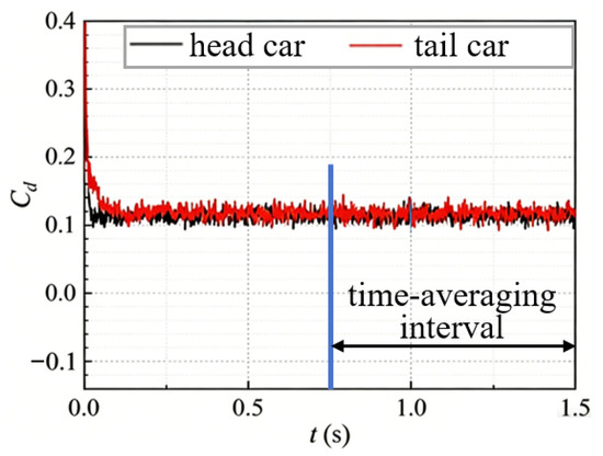
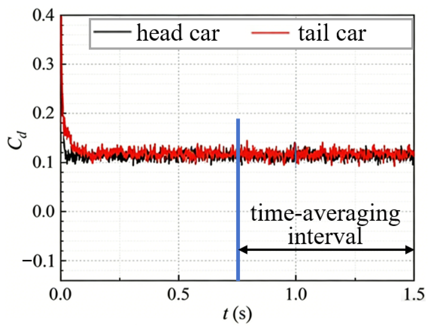
Figure 1 presents the time histories of the aerodynamic drag coefficients for the head and tail cars of the high-speed train at an operational speed of 100 m/s. As shown, the aerodynamic drag exhibits continuous temporal fluctuations. Nevertheless, after an initial transient period, the drag coefficients transition into a steady state, sustaining fluctuations within a stable range. To ensure the complete dissipation of initial transient effects, the first 1.0 s of the simulation was discarded. The subsequent 0.5 s window—corresponding to approximately 5 complete flow passes over the scaled train length and encompassing approximately 8 to 29 sweeping periods of the SWJ actuator (depending on the evaluated jet velocities)—was utilized for time-averaging the statistical data. This duration ensures statistically stable mean quantities and provides a reliable basis for stable aerodynamic evaluations.

Figure 1. Time–history curve of the aerodynamic drag coefficient for a high-speed train.

The aerodynamic drag coefficient C_d and the pressure coefficient C_p were calculated as follows:

$$C_d={\displaystyle \frac{F_d}{0.5\rho U_{\infty }^{2}S}}$$

(2)

$$C_p={\displaystyle \frac{(p-p_{\infty })}{0.5\rho U_w^2}}$$

(3)

where F_d is the aerodynamic drag, ρ is the air density, U_∞ is the incoming flow velocity, S is the projected cross-sectional area of the train, p is the surface pressure, p_∞ is the reference pressure, and U_w is the incoming wind speed in the wind-tunnel test. The drag-reduction rate is defined as η = (C_d,0 − C_d,c)/C_d,0 × 100%, where C_d,0 and C_d,c are the drag coefficients before and after control, respectively.

The Reynolds number (Re) is a fundamental dimensionless quantity in fluid mechanics, defined as the ratio of inertial forces to viscous forces within a fluid subjected to relative internal movement. It serves as a critical criterion for predicting flow regimes, specifically for distinguishing between laminar and turbulent flows. Mathematically, it is expressed as:

$$Re={\displaystyle \frac{\rho U{L}_c}{\mu }}={\displaystyle \frac{U{L}_c}{\nu }}$$

(4)

where ρ denotes the air density (1.225 kg/m³), U represents the macroscopic incoming flow velocity (100 m/s), Lc indicates the characteristic length (adopted as the height of the 1:8 scaled train model, H = 0.5062 m), and μ and ν signify the dynamic (1.794 × 10⁻⁵ Pa·s) and kinematic viscosities of the fluid, respectively. Based on these specified parameters, the operating Reynolds number is approximately 3.457 × 10⁶. Although this value is inherently lower than that of a full-scale operational train, it has well exceeded the critical threshold for the Reynolds-independent regime in bluff-body aerodynamics, ensuring that the simulated flow structures remain representative of full-scale conditions. This high Reynolds number indicates a fully developed, highly turbulent flow field around the trainset, thereby justifying the employment of the IDDES framework for the numerical simulations.

2.2. Geometric Model

2.2.1. High-Speed Train Model

A three-car high-speed train was used as the basic model, including a head car, a middle car, and a tail car. The geometry was simplified to eliminate redundant features, while key structures such as bogies and windshields were retained, as shown in Figure 2. To avoid the influence of model scaling on the length unit, the train height H = 4.05 m was used for nondimensionalization. The length of the three-car train model was 20.11 H.

Figure 2. Three-car high-speed train model.

2.2.2. Simplified Sweeping-Jet Oscillator Model

Resolving the micro-geometric details of the sweeping-jet oscillator within the macroscopic train domain presents a large spatial scale disparity, which would otherwise impose excessive grid resolution requirements and computational costs. To address this challenge, this study introduces a novel simplified modeling strategy for the SWJ. As illustrated in Figure 3, the complex internal fluidic channels of the oscillator were bypassed; instead, only the jet outlet and the expansion chamber were retained to construct an equivalent sweeping-jet model.

Figure 3. Simplified geometric model of the jet oscillator.

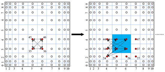
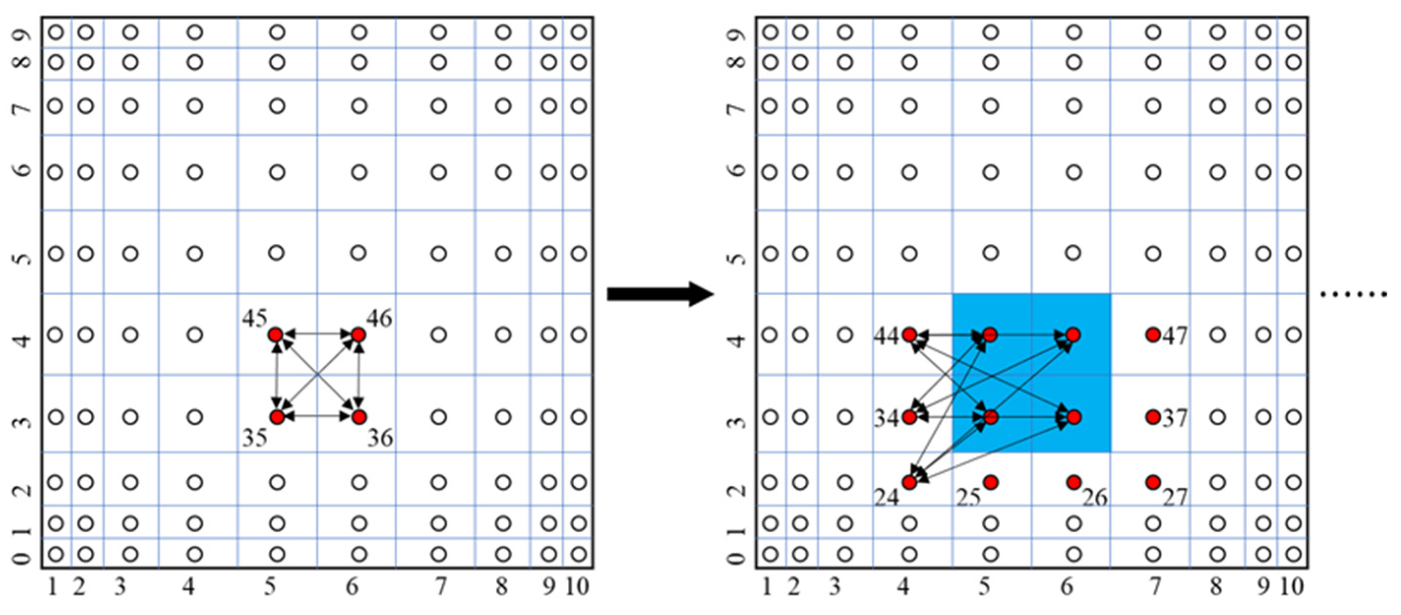
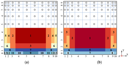
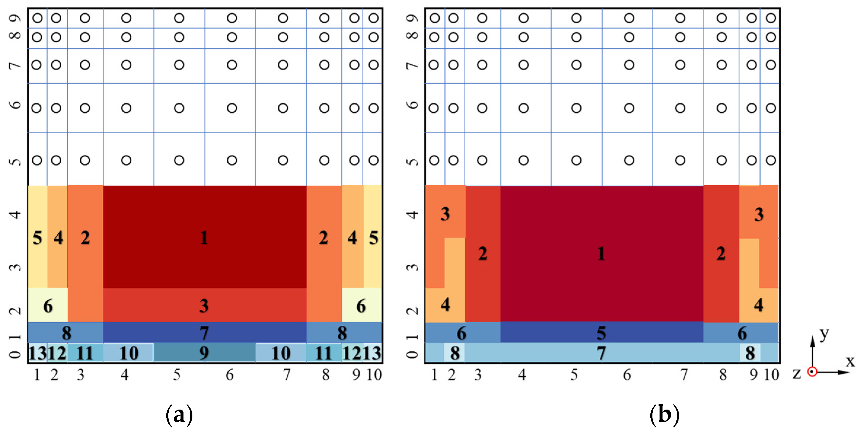
The outlet velocity is described by fitting functions in different velocity-similar regions. Figure 4 shows the division method, and Figure 5 shows the partitions of the velocity components vy and vz. The velocity component vy at the outlet is symmetric in the upper and lower parts, but the signs are opposite. For this reason, the upper regions are marked with y+ and the lower regions are marked with y−. The fitting functions of the lower regions have the opposite signs and a half-period shift compared with the upper regions. The specific mathematical expressions of the fitting functions for the velocity components vy and vz in the selected regions are detailed in Table 1 and Table 2, respectively.

Figure 4. Division method for velocitysimilar regions. The red circles represent the identified velocity-similar measuring points, and the blue frame indicates the merged region of these similar points.

Figure 5. Division of velocity-similar regions: (a) vy and (b) vz. The numbers indicate the designated velocity-similar regions, and different colors are used to visually distinguish these regions.

Table 1. Fitting functions for velocity component vy in selected velocity-similar regions.

Region	Fitting Function
1-y+	4.972 − 29.43 × cos(460.4t + acos(−1)) − 3.555 × sin(460.4t + acos(−1))
1-y−	−(4.972 − 29.43 × cos(460.4t) − 3.555 × sin(460.4t))
5-y+	5.85 − 51.98 × cos(460.4t + acos(−1)) − 22.67 × sin(460.4t + acos(−1))
5-y−	−(5.85 − 51.98 × cos(460.4t) − 22.67 × sin(460.4t))
7-y+	15.99 − 22.42 × cos(460.4t + acos(−1)) − 4.123 × sin(460.4t + acos(−1))
7-y−	−(15.99 − 22.42 × cos(460.4t) − 4.123 × sin(460.4t))
10-y+	6.691 − 5.702 × cos(921t + acos(−1)) − 1.852 × sin(921t + acos(−1))
10-y−	−(6.691 − 5.702 × cos(921t) − 1.852 × sin(921t))

Table 2. Fitting functions for velocity component vz in selected velocity-similar regions.

Region	Fitting Function
1	49.58 − 1.56 × cos(924.1t) − 0.2597 × sin(924.1t)
3	35.17 + 1.272 × cos(1840t) + 0.2256 × sin(1840t)
5	47.13 + 1.804 × cos(919.3t) − 0.7836 × sin(919.3t)
8	30.83 + 9.75 × cos(921.4t) + 3.37 × sin(921.4t)

Under the same meshing strategy, the total cell count for a single equivalent model was only approximately 5% of that for a complete fluidic oscillator, which substantially reduced the overall computational cost. Therefore, the equivalent model was utilized in place of the fully resolved fluidic oscillator in the subsequent simulations.

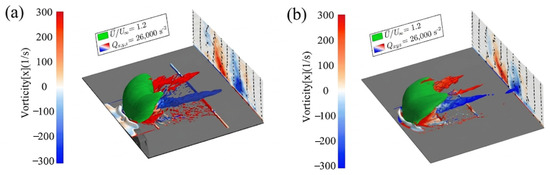
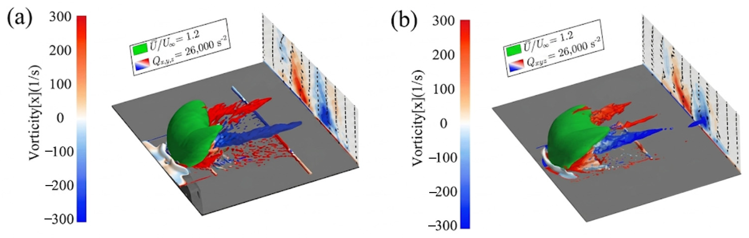
The accuracy of the aforementioned simplified method was verified both qualitatively and quantitatively. The velocity discrepancy at each monitoring point across the throat exit surface was less than 5%. Furthermore, the transient sweeping behavior of the jet closely resembled that of the complete model in a time-resolved manner, as demonstrated in Figure 6.

Figure 6. Comparison of time-averaged velocity isosurfaces and Q-criterion isosurfaces between the two oscillator models: (a) complete model; (b) equivalent simplified model.

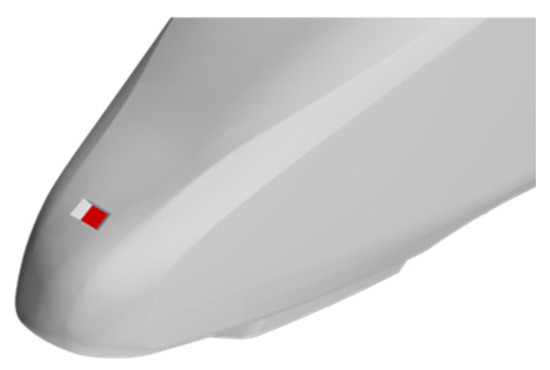
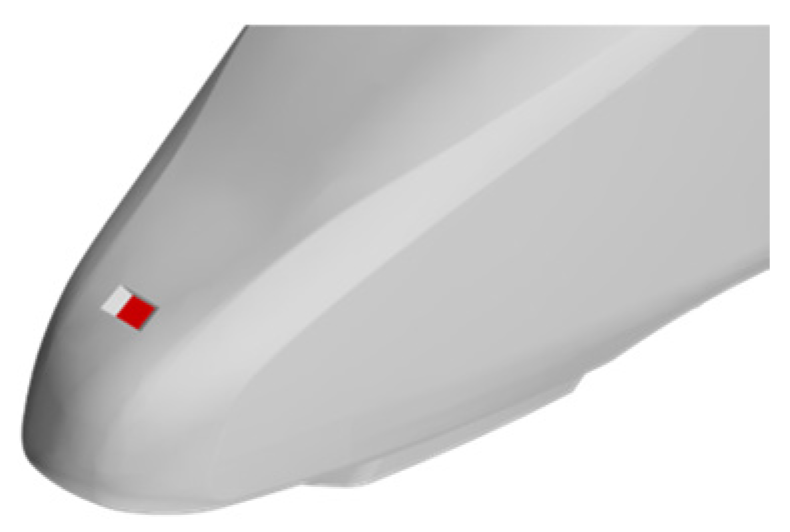
The spatial arrangement of the SWJ oscillator on the head car is guided by fundamental train aerodynamics. Because the streamlined nose experiences severe flow stagnation and positive pressure accumulation, the oscillator is strategically positioned at the nose tip to actively manipulate the local flow development. As illustrated in Figure 7, this setup aims to inject a spatially oscillating jet into the oncoming stream to establish a fluidic buffer zone. This configuration is hypothesized to alter the attached flow trajectory, thereby mitigating the localized high-pressure concentration.

Figure 7. Installation position of the sweeping-jet oscillator on the head car.

2.3. Computational Domain and Boundary Conditions

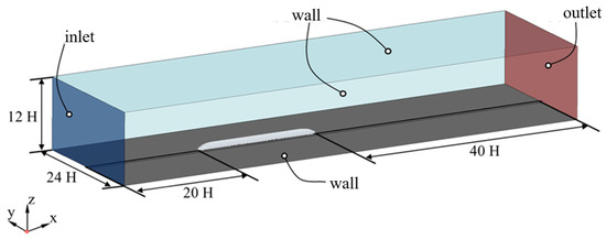
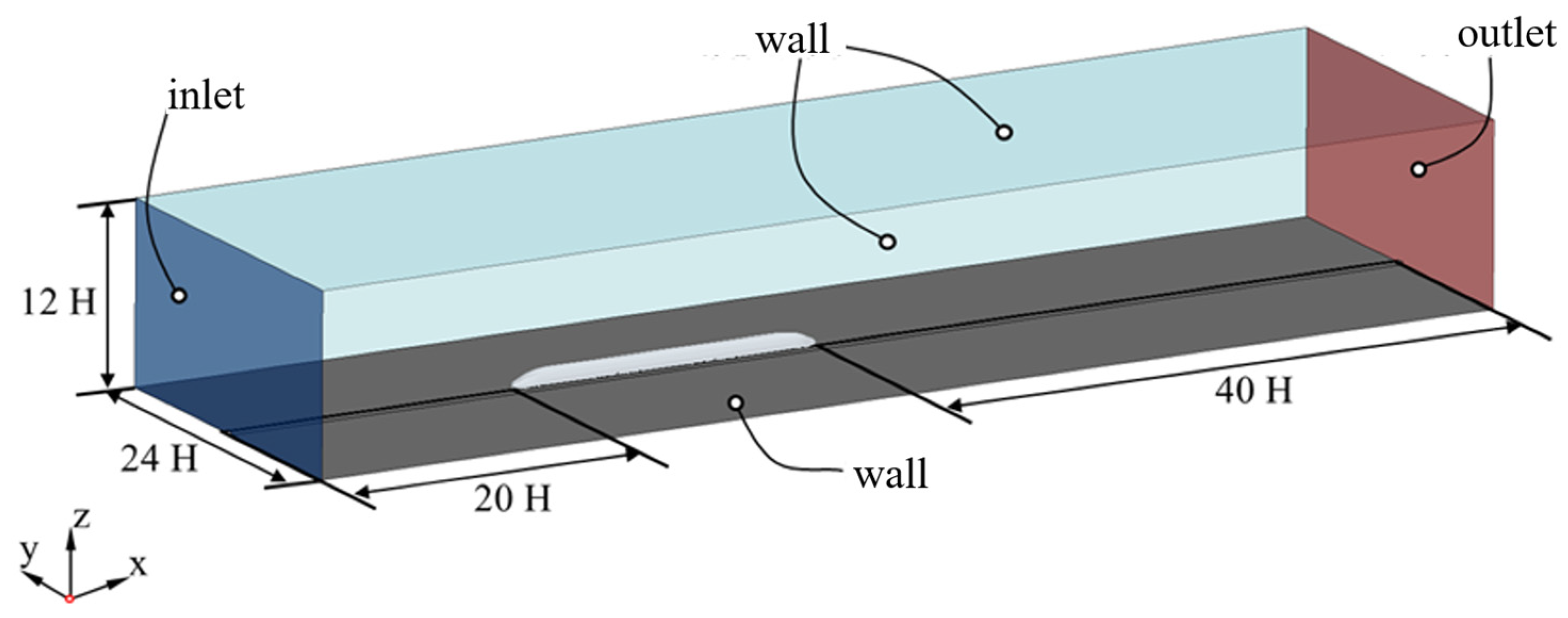
The computational domain and boundary conditions are shown in Figure 8. A 1:8 scaled model was used to meet the near-wall grid requirement of the selected turbulence model. The velocity inlet was located 20 H in front of the train, and the pressure outlet was located 40 H behind the train. The incoming flow velocity was the same as the train speed, which was 100 m/s, or about 360 km/h. The ground and rails were set as moving walls with the same velocity as the incoming flow. The top and side surfaces of the computational domain were set as slip walls. The total width and height of the computational domain were 24 H and 12 H, respectively, and the rail track passed through the whole domain. This extensive domain size was specifically configured to ensure that the artificial boundaries do not impose spurious pressure gradients or constrain the downstream wake development. The resulting blockage ratio was about 1%, which is well below the generally recommended threshold of 5% in vehicle aerodynamics, eliminating artificial flow acceleration effects and justifying the reliability of the domain setup.

Figure 8. Computational domain for the high-speed train simulation.

2.4. Mesh Generation and Numerical Settings

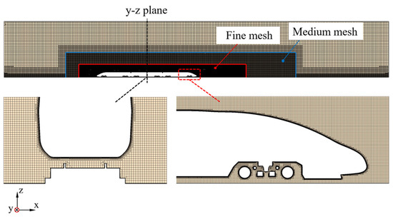
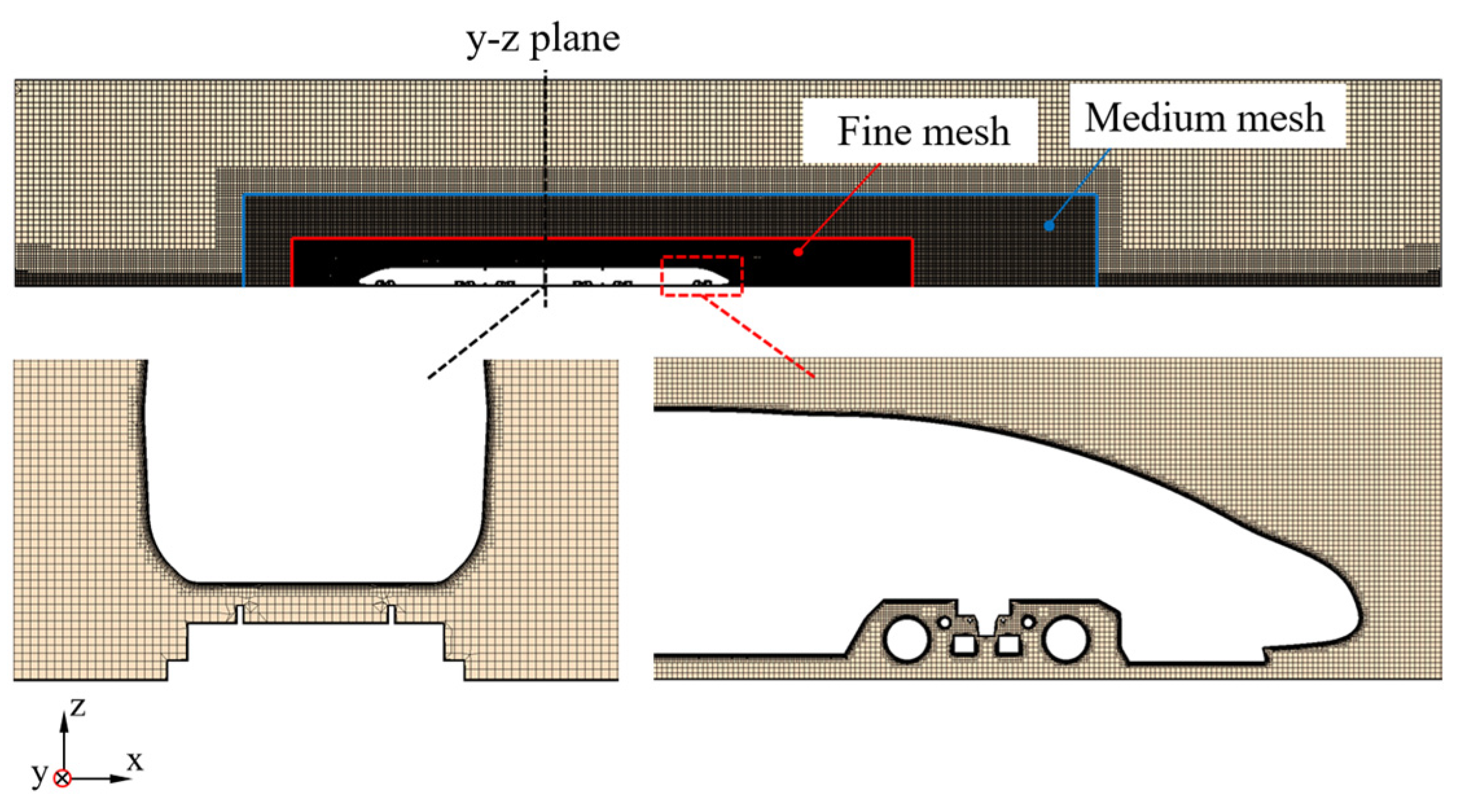
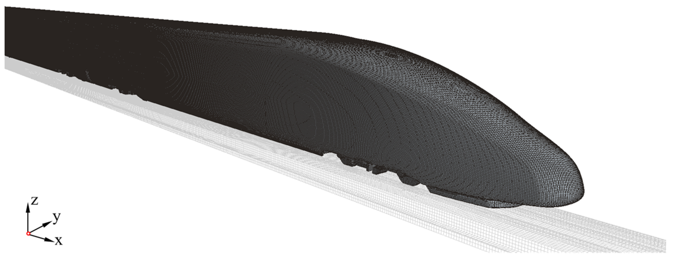
The computational domain was discretized using STAR-CCM+ (v14.02, Siemens Digital Industries Software, Plano, TX, USA). Unstructured hexahedral meshes were generated. Figure 9 shows the mesh in the computational domain, and Figure 10 shows the surface mesh of the train. The surface mesh size of the train was 40 mm. Two refined volume-mesh regions were set around the train, with sizes of 80 mm and 160 mm. A medium-size transition region was used between fine and coarse meshes to obtain a smooth transition. Twelve prism layers were generated on the train surface. The first layer thickness was 3 mm, the growth factor was 1.2, and the total prism-layer thickness was 75 mm. Based on this initial layer configuration, the average y⁺ value across the train surface ranged from approximately 30 to 70. Within the IDDES framework, the near-wall boundary layer is inherently governed by the RANS mode. Given the large Reynolds number in this study, resolving the viscous sublayer (y⁺ ≈ 1) would incur prohibitive computational costs. Therefore, the "all y⁺ wall treatment" was employed.

Figure 9. Mesh of the computational domain. The black dashed line indicates the position of the cross-sectional view on the y–z plane (bottom left), and the red dashed frame indicates the zoomed-in view of the local mesh around the train head (bottom right).

Figure 10. Surface mesh of the high-speed train.

This hybrid approach blends the viscous sublayer formulation with standard wall functions, ensuring accurate predictions of near-wall shear stresses even when the first grid cell falls within the buffer or logarithmic regions. This mesh resolution satisfies the near-wall modeling requirements of the IDDES approach.

2.5. Grid-Independence Study

Three meshes were generated for the train model: a coarse mesh, a medium mesh, and a fine mesh. The purpose was to reduce the influence of grid resolution on the numerical results. The cell numbers and main mesh settings are listed in Table 3. The mesh sizes in the table are the original full-scale values before model scaling.

Table 3. Mesh strategies used in the grid-independence study.

Mesh Strategy	Number of Cells (104)	Surface Mesh Size (mm)	Volume Mesh Size (mm)
Coarse	1936	80	160
Medium	3783	40	80
Fine	9339	20	40

Table 4 compares the aerodynamic drag coefficients and errors for different mesh strategies. The total drag coefficient of the coarse mesh differs from that of the fine mesh by 12.85%. This accuracy is not enough for the present study. The total drag coefficient of the medium mesh differs from that of the fine mesh by 4.37%, which is lower than 5%. Therefore, considering both the accuracy and the computational cost, the medium mesh was used in the following simulations.

Table 4. Aerodynamic drag coefficients and errors for different mesh strategies and wind-tunnel test.

Strategy	Head	Error (%)	Middle	Error (%)	Tail	Error (%)	Whole	Error (%)
Coarse mesh	0.1063	−10.45	0.0696	−20.22	0.1096	−8.58	0.2855	−12.85
Medium mesh	0.1134	−4.41	0.0829	−4.96	0.1169	−2.54	0.3133	−4.37
Fine mesh	0.1195	-	0.0872	-	0.1199	-	0.3276	-
Wind tunnel	0.1180	-	-	-	-	-	-	-

It is crucial to clarify that the reported 4.37% grid uncertainty represents the absolute discrepancy in the baseline drag coefficient between the medium and fine meshes. However, when evaluating the active flow control efficacy, the relative drag reduction rate is calculated by comparing the actuated cases against the baseline under an identical mesh topology. Since the grid architecture remains completely unchanged outside the immediate vicinity of the sweeping-jet oscillator. Using the same mesh topology for the baseline and controlled cases reduces inconsistencies associated with changes in grid construction. However, correlated discretization errors are not assumed to cancel completely. The reported drag-reduction rates should be interpreted as medium-grid estimates. Therefore, the medium mesh is demonstrated to be sufficiently robust and adequate for capturing the relative aerodynamic variations induced by the active flow control.

2.6. Wind-Tunnel Validation

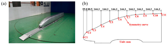
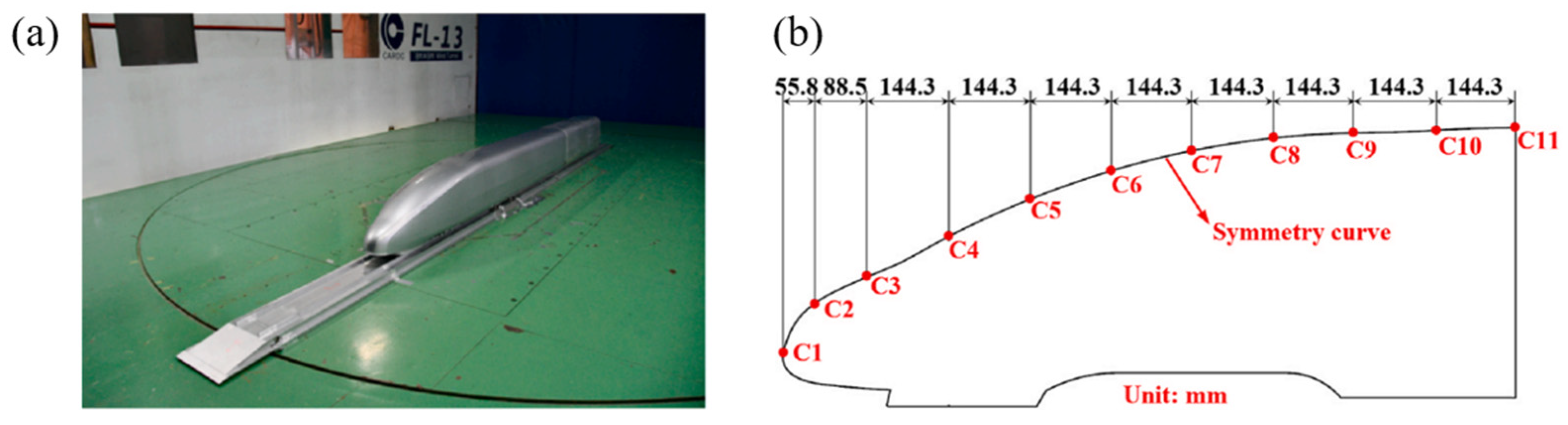
The wind-tunnel test was carried out in the wind tunnel of the China Aerodynamics Research and Development Center. The incoming wind speed was 45 m/s, and the Reynolds number was 1.55 × 10⁶. A special test platform, the same as that used by Zhang et al. [26], was used to reduce the influence of the ground boundary layer on the test data. A 1:8 scaled one-and-a-half-car model was used to test the aerodynamic performance of the head car. The model and the installation position are shown in Figure 11a. The blockage ratio of the test was about 0.8%, which was much lower than 5%. Therefore, blockage correction was not applied. Figure 11b shows the pressure taps along the centerline of the streamlined head region.

Figure 11. Wind-tunnel test and related settings: (a) test model and installation; (b) pressure-tap arrangement.

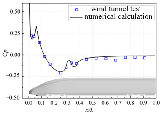
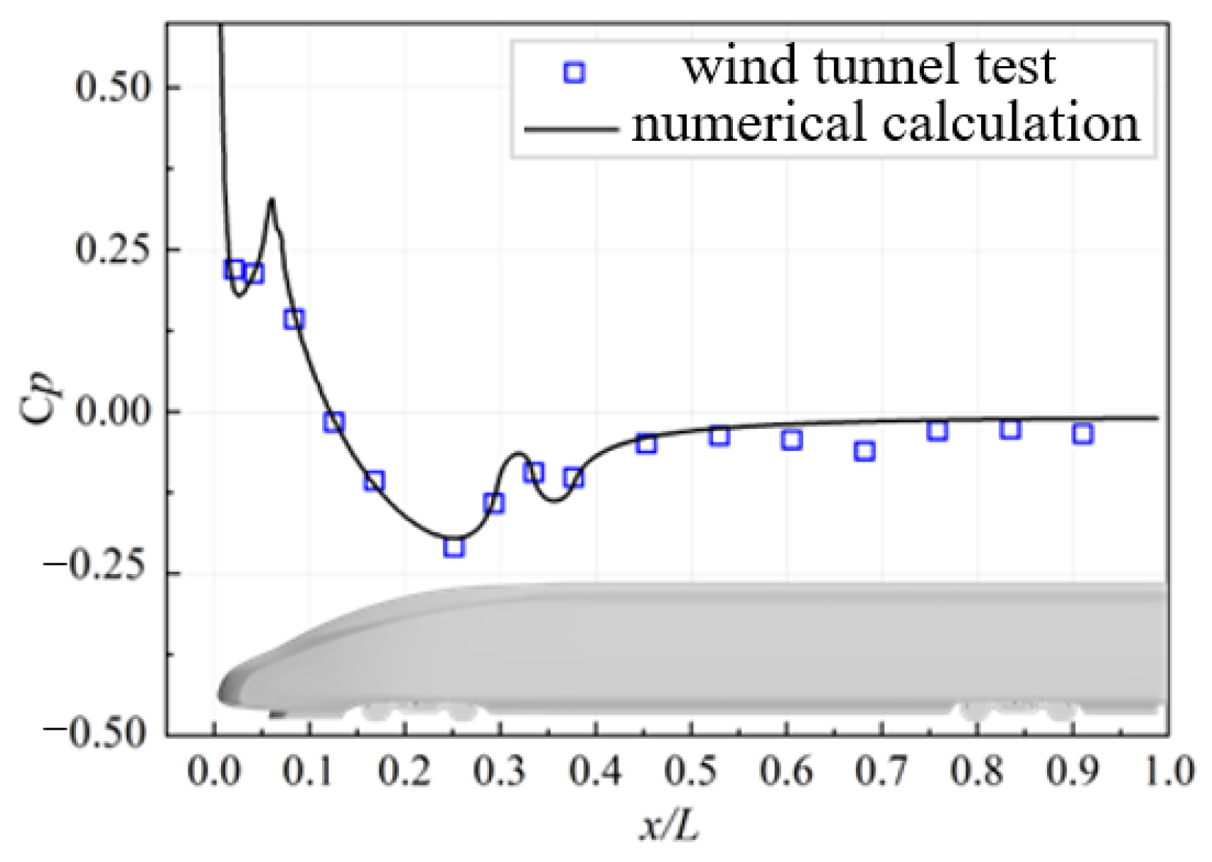
Figure 12 compares the pressure coefficient distribution along the centerline of the head car between the wind-tunnel test and the numerical simulation. The numerical pressure coefficient agrees well with the measured pressure coefficient, although small differences exist at some measurement points. Notably, due to experimental limitations, the validation process was conducted solely on the baseline configuration of the head car. Furthermore, the wind tunnel test adopted a fixed ground boundary, whereas the numerical simulation utilized a moving ground boundary. This difference can be partially attributed to the minor discrepancy in the drag coefficient. This validation aims to demonstrate the accuracy of the fundamental numerical platform in capturing the complex flow characteristics around high-speed trains, thereby providing a reliable baseline reference for the subsequent research on active flow control using sweeping jets.

Figure 12. Pressure coefficient distribution along the centerline of the head car.

In addition, the drag coefficient of the head car obtained by the medium mesh differs from the wind-tunnel result by 3.87%. The main reason for the difference was that the boundary conditions were not exactly the same. In the simulation, the ground and rails were moving walls, while they were fixed walls in the wind-tunnel test. In general, the numerical error was within an acceptable range for the present study.

2.7. Simulation Cases

As an initial exploratory effort to implement sweeping-jet configurations on high-speed trains, this study aims to systematically explore the flow-control efficacy of different operational parameters on key localized regions. Ultimately, these preliminary parametric investigations are intended to provide a reliable methodological reference for the future deployment of such active flow control systems across broader vehicular domains. To achieve this, the simulation cases are categorized into three major groups, as summarized in Table 5. The first group evaluates the effects of the sweeping-jet model size, which is nondimensionalized by the ratio of the jet outlet width (d_h) to the train width (W = 0.83 H). The second and third groups investigate the influences of varying jet deflection angles and jet velocities, respectively.

Table 5. Summary of the simulation cases and parameter settings.

Research Objectives	Case No.	Sweeping-Jet Model Size (dh/W)	Sweeping-Jet Angle	Sweeping-Jet Velocity
Effect of different sweeping-jet sizes	S1	2:50	150°	25 m/s
	S2	3:50
	S3	4:50
	S4	5:50
Effect of different sweeping-jet angles	A1	5:50	180°	25 m/s
	A2		150°
	A3		120°
	A4		90°
Effect of different sweeping-jet velocities	V1	5:50	120°	10 m/s
	V2			15 m/s
	V3			20 m/s
	V4			25 m/s
	V5			30 m/s
	V6			35 m/s

2.8. Considerations for Energy Efficiency and Practical Feasibility

The equivalent sweeping-jet model used in the present simulations prescribes the time-resolved velocity field at the jet exit and does not resolve the complete supply plenum, feedback channels, ducts, compressor, or motor. Therefore, the electrical input power of a practical actuation system cannot be determined directly. To distinguish the quantities that can and cannot be evaluated from the present numerical framework, the gross aerodynamic power saving is first defined as

$$P_{save}=(F_{D,0}-F_{D,c})U_{\infty }=0.5\rho {U_{\infty }}^{3}S\Delta C_D$$

(5)

The mechanical power delivered to the external flow through the jet exit is evaluated from the time-averaged mechanical-energy flux:

$$P_{j,\mathrm{flow}}={\displaystyle \frac{1}{T}}{\displaystyle {\int }_0^T{\displaystyle {\int }_{A_j}\left[(p_j-p_{\infty })+\frac{1}{2}\rho |u_j{|}^2\right]}}(u_j\cdot n)dAdt$$

(6)

where A_j is the total jet-exit area and n is directed into the external-flow domain. The pressure-work term is retained because the actuator is installed in a positive-pressure region near the nose stagnation zone. The corresponding jet-flow power coefficient and power-gain ratio are defined as

$$C_{P,j,\mathrm{flow}}={\displaystyle \frac{P_{j,\mathrm{flow}}}{0.5\rho U_{\infty }^{3}S}},\hspace{1em}{G}_{\mathrm{flow}}={\displaystyle \frac{P_{\mathrm{save}}}{P_{j,\mathrm{flow}}}}={\displaystyle \frac{\Delta C_D}{C_{P,j,\mathrm{flow}}}}$$

(7)

G_flow is a power-gain ratio rather than a thermodynamic efficiency and is therefore not bounded by unity. Moreover, P_j,flow does not include the internal pressure losses of the fluidic oscillator or the conversion losses of the complete supply system. Consequently, the actual electrical input power is higher than the value reported here. The present analysis therefore provides a lower-bound estimate of the fluid power requirement and a balance criterion, rather than direct evidence of positive net electrical power saving.

3. Results and Discussion

3.1. Baseline Aerodynamic Drag Characteristics

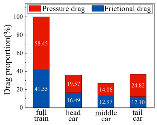
Because the middle car has a different shape and position from the head and tail cars, the aerodynamic drag distribution is not uniform along the train. Figure 13 shows the drag distribution of the train.

Figure 13. Aerodynamic drag distribution of the high-speed train.

Specifically, the head, middle, and tail cars account for approximately 36%, 27%, and 37% of the total drag, respectively, exhibiting a distinct U-shaped distribution pattern. According to the formation mechanism, the total aerodynamic drag can be divided into friction drag and pressure drag. Their proportions are 41.55% and 58.45%, respectively. Specifically, the pressure drag constitutes 19.57% of the total drag for the head car, and 24.82% for the tail car. Furthermore, within the tail car’s individual aerodynamic resistance, the pressure drag dominates over the friction drag. Therefore, the pressure drag of the head and tail cars is the main source of the total drag. Sweeping-jet drag reduction should first focus on reducing the pressure drag in these regions.

3.2. Flow Structures Around the High-Speed Train

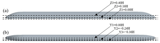
Understanding the flow field around the train is the basis for aerodynamic drag reduction. To show the velocity and pressure distributions around the train, different body sections were selected. Figure 14 shows the section positions. Y1–Y3 are longitudinal sections at y = 0 H, y = −0.24 H, and y = −0.36 H, respectively. Z1–Z3 are horizontal sections at z = 0 H, z = 0.16 H, and z = 0.40 H, respectively.

Figure 14. Section positions of the high-speed train: (a) side view; (b) top view.

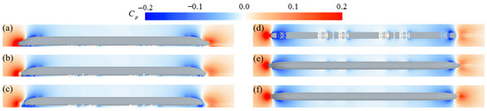
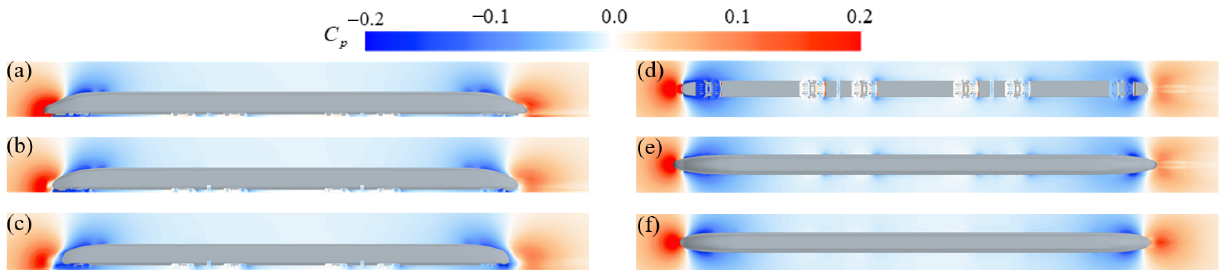
Figure 15 shows the time-averaged pressure contours in different longitudinal and horizontal sections. The pressure is expressed in a dimensionless form via the pressure coefficient (C_p). The pressure field around the train can be divided into five main regions. The first region is the positive-pressure region at the front of the head car, where the incoming flow is blocked and compressed by the train body. The second region is the negative-pressure region near the transition between the streamlined head and the equal-section body. In this region, the increase in body cross-section accelerates the flow and decreases the pressure. The third region is the equal-section body region, where the body shape changes little and the pressure variation is small. The fourth region is the negative-pressure region near the transition between the equal-section body and the streamlined tail. The local decrease in body cross-section accelerates the flow and lowers the pressure. The fifth region is the weak positive-pressure region near the tail nose, where the interaction of the wake shear layers reduces the flow velocity. The pressure regions near the head car are larger than those near the tail car, which shows that the streamlined shape has an important influence on the pressure distribution.

Figure 15. Time-averaged pressure contours in different sections: (a) Y1 = 0 H; (b) Y2 = −0.24 H; (c) Y3 = −0.36 H; (d) Z1 = 0 H; (e) Z2 = 0.16 H; (f) Z3 = 0.40 H.

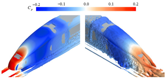
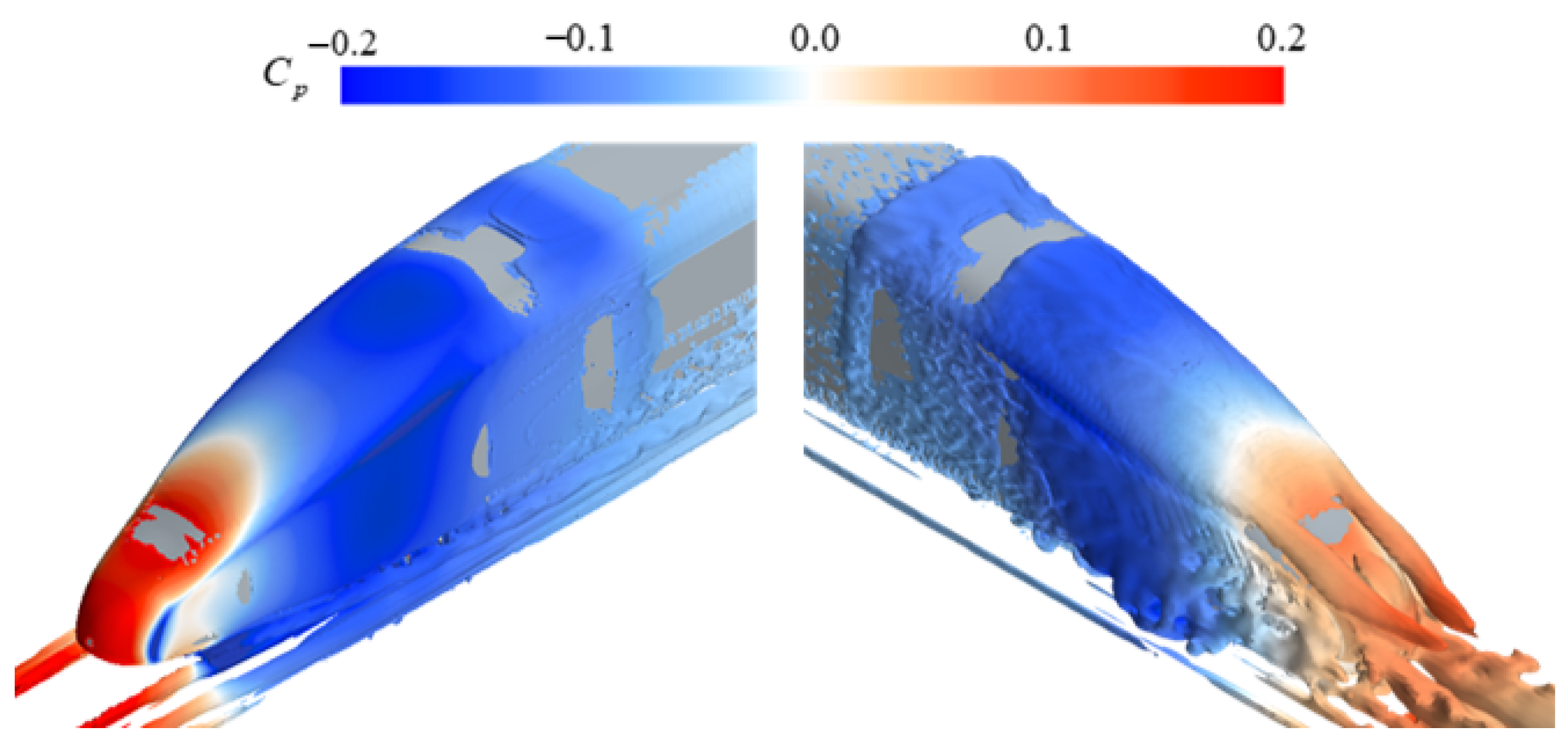
Figure 16 shows the time-averaged pressure distribution and the Q-isosurface with Q = 5000 s⁻² around the head and tail cars. For the head car, the positive-pressure region is mainly located at and above the nose tip, where the pressure coefficient exceeds 0.2. Negative-pressure regions appear on both sides of the nose, above the driver cab, and near the transition between the streamlined region and the equal-section body. The pressure coefficient in these regions drops below −0.2. The Q-isosurface shows that only a few vortices exist around the head car. Therefore, sweeping-jet control on the head car should mainly target the strong positive-pressure region at the head to reduce the pressure drag of the whole train.

Figure 16. Time-averaged Q-isosurfaces around the head and tail cars, colored by the pressure coefficient.

For the tail car, the positive-pressure region is located near the tail nose, while the largest negative-pressure region is located in the upper part of the streamlined region and near the transition region. As the flow moves downstream, large-scale vortices form on both sides of the upper surface of the tail car and separate near the lower edge of the windshield. A larger streamwise vortex also appears downstream of the nose tip. These vortices are mainly distributed in the negative-pressure region and separate near the boundary between the positive- and negative-pressure regions. This provides a reference for the arrangement of sweeping jets.

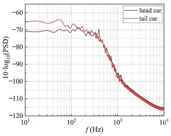
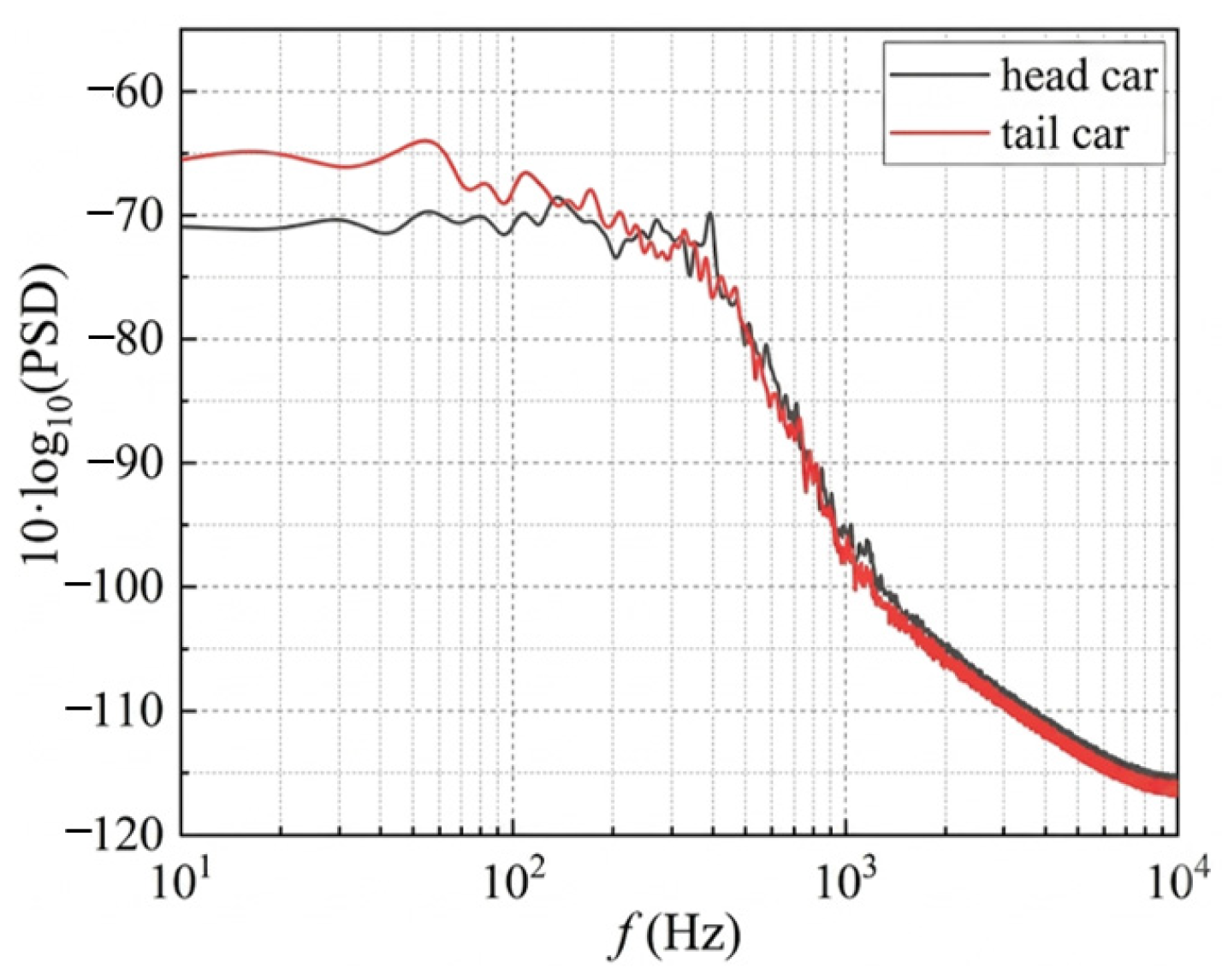
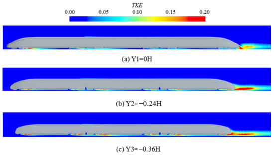
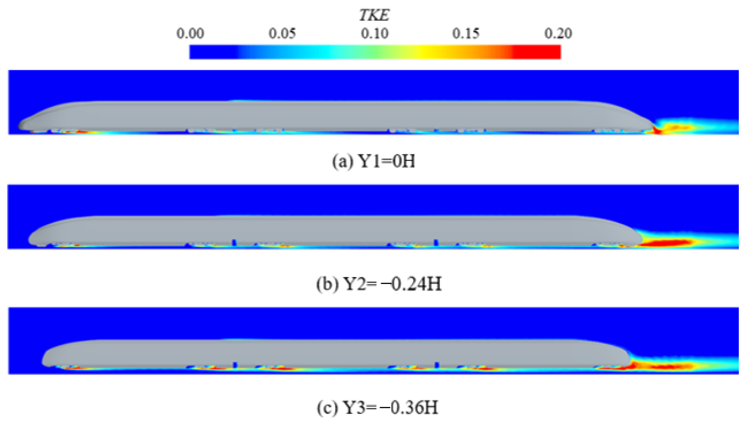
To quantitatively evaluate the unsteady wake characteristics, the power spectral density (PSD) of the aerodynamic drag coefficients and the turbulent kinetic energy (TKE) around the train were analyzed. As shown in Figure 17, the PSD curves reveal distinct multimodal characteristics.

Figure 17. Power spectral density (PSD) curves of the aerodynamic drag coefficients for the head and tail cars.

The dominant modal frequency for the tail car is approximately 54 Hz, which is significantly lower than that of the head car (136 Hz). This quantitatively demonstrates the existence of larger-scale, low-frequency shedding vortices dominating the tail wake region, as larger vortical structures inherently exhibit lower shedding frequencies.

Furthermore, to quantify the spatial energy distribution of these wake vortices, Figure 18 displays the normalized TKE contours at different longitudinal sections. The high-TKE regions are predominantly localized behind the tail nose. Notably, as the lateral distance increases, the scope of the highly turbulent region expands and then contracts, reaching its maximum extent near the longitudinal section of Y = −0.24 H, where the peak TKE value clearly exceeds 0.2. This specific localization provides a spatial scale and energy boundary for the large-scale trailing vortices, thereby quantitatively justifying the target regions for the active flow control setup.

Figure 18. Normalized turbulent kinetic energy (TKE) contours at different longitudinal sections of the train.

In summary, the baseline simulation results support the control hypotheses formulated in Section 2.2.2. The time-averaged pressure distribution confirms that the severe positive-pressure stagnation zone localized at the head-car nose tip dominates the overall pressure drag. This prominent flow feature provides clear empirical evidence that supports the targeted spatial arrangement of the sweeping jet, indicating that active aerodynamic control should strategically focus on these specific flow hot spots.

3.3. Effects of Sweeping-Jet Model Size

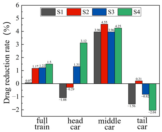
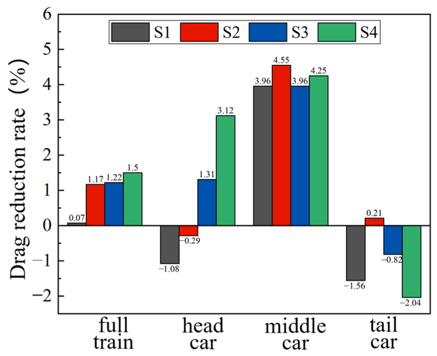
The model size is an important parameter for sweeping-jet flow control. According to the baseline aerodynamic characteristics and the initial arrangement of the jets, four outlet-width ratios were considered. The size was nondimensionalized by the ratio between the jet outlet width dh and the train width W, where W = 0.83 H. The four cases were 2:50 (S1), 3:50 (S2), 4:50 (S3), and 5:50 (S4), as shown in Figure 19. The baseline case without control was named S0. For all four size cases, the sweeping-jet equivalent models were placed at the same position. The bulk jet velocity U_bulk was 25 m/s, or 0.25U_∞. The jet direction was normal to the local train surface.

Figure 19. Sweeping-jet model-size cases: (a) S1; (b) S2; (c) S3 and (d) S4. The red region represents the jet exit.

Figure 20 shows the drag-reduction rate of the train under different sweeping-jet model sizes. All four configurations effectively decrease the total aerodynamic drag of the three-car train. In general, the larger the sweeping-jet model is, the stronger the drag reduction becomes. Under the S4 configuration, the total drag reduction in the three-car train is approximately 1.5%. The head-car drag reduction also increases with model size. When the size is S4, the head-car drag reduction reaches 3.12%. The middle car shows good drag reduction in all four size cases, and the maximum reduction reaches 4.55%. However, the tail car shows drag increase in most cases, with the largest drag increase of 2.04%.

Figure 20. Drag-reduction rate of the high-speed train under different sweeping-jet model sizes.

The drag penalty observed on the tail car can be interpreted as a downstream consequence of the nose-mounted sweeping jet. Although the jet reduces the stagnation pressure on the head car by lifting the oncoming flow and forming a low-speed recirculation region, it also modifies the boundary-layer development along the train body. The flow convected toward the tail car may therefore have a thicker low-momentum region and stronger three-dimensional disturbance than that in the baseline case. For the tail car, aerodynamic drag is strongly associated with pressure recovery over the streamlined tail and with the wake vortical structures. A lower-momentum incoming boundary layer is less able to withstand the adverse pressure gradient around the tail transition, which may enlarge the low-pressure region and strengthen the wake deficit. Consequently, the pressure drag of the tail car can increase even when the total drag of the three-car train is reduced.

The sweeping jet has a stronger influence on the aerodynamic characteristics of the head and middle cars. Figure 21 shows the time-averaged velocity contours and streamlines in the center longitudinal section of the head car under different model sizes. Because of the sweeping jet, the incoming flow is lifted at the position of the jet outlet. A low-speed recirculation region appears above the train surface behind the jet outlet. This region weakens the direct impact of the incoming flow on the train body and reduces the local surface pressure. In addition, increasing the size of the sweeping jet model leads to a higher mass flow rate and a broader range of influence, which consequently enlarges the low-speed recirculation zone. Conversely, a smaller jet size is insufficient to sustain a stable low-speed recirculation zone, yielding negligible improvements in pressure drag. More importantly, this inadequate jet disrupts the inherent streamlined profile of the head car, ultimately resulting in an aerodynamic penalty where the drag increases instead of decreasing.

Figure 21. Time-averaged velocity contours and streamlines in the center longitudinal section of the head car under different sweeping-jet model sizes: (a) S1; (b) S2; (c) S3 and (d) S4.

3.4. Effects of Sweeping-Jet Angle

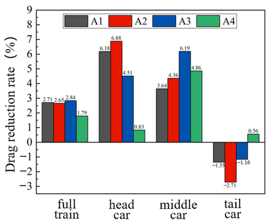
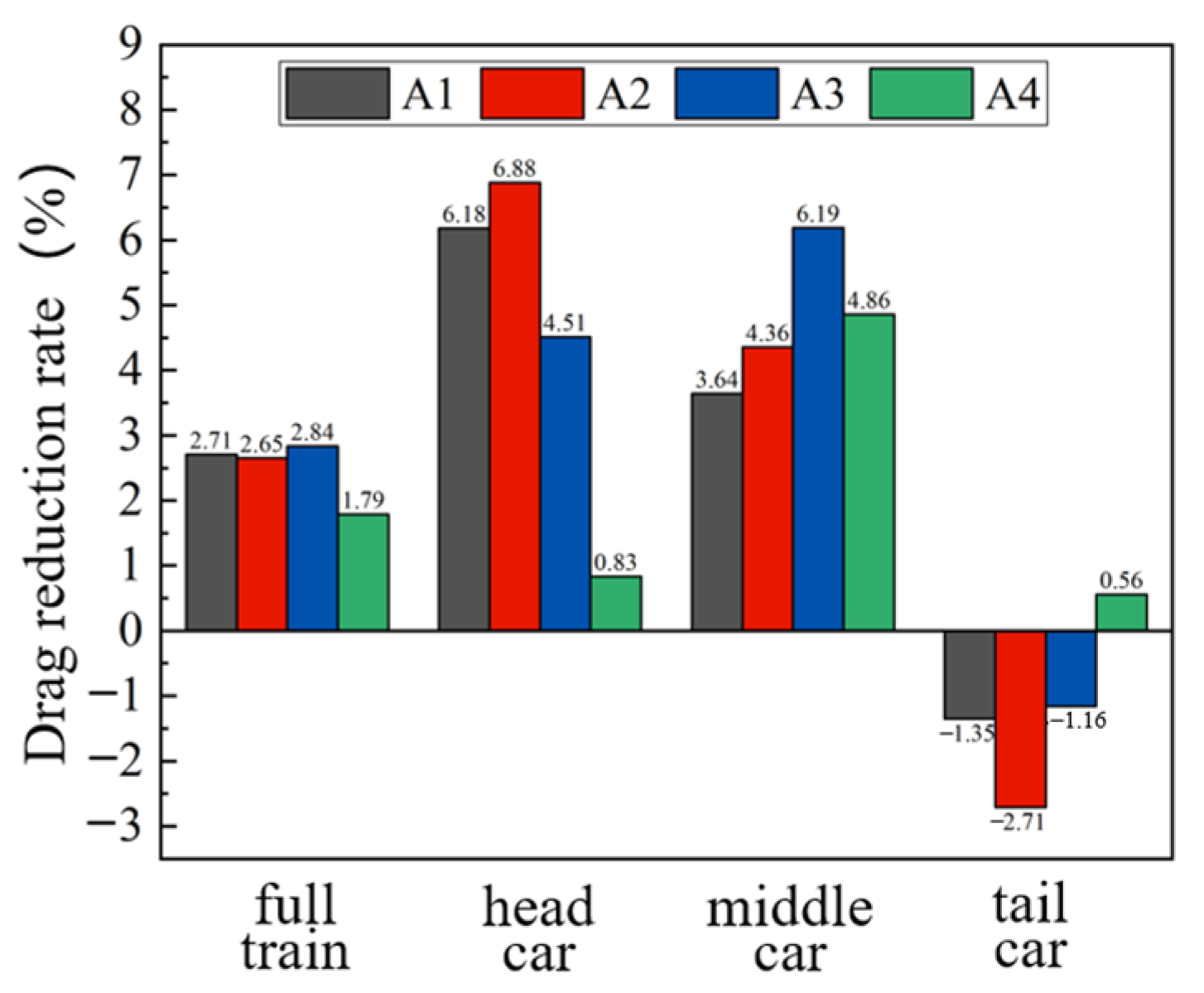
The sweeping-jet angle has a clear influence on the low-speed recirculation region behind the jet outlet. Four jet angles were considered. Using the incoming flow direction as the reference, the jet directions were 180° (A1), 150° (A2), 120° (A3), and 90° (A4), as shown in Figure 22 (where the blue and red arrows denote the incoming flow and jet directions, respectively). The baseline case without control was named A0. The four cases used the same model size, the same position, and the same bulk jet velocity U_bulk = 25 m/s = 0.25U_∞.

Figure 22. Sweeping-jet angle cases: (a) A1; (b) A2; (c) A3 and (d) A4.

Figure 23 shows the drag-reduction rate of the train under different sweeping-jet angles. All four angles reduce the total aerodynamic drag of the three-car train to some extent. The total drag reductions of A1, A2, and A3 are close to each other, while that of A4 is lower. This indicates that the jet angle has a relatively small influence on the total drag reduction in the three-car train. For the head car, the drag-reduction rate first increases and then decreases as the angle changes. The drag reduction in the head car is the smallest in A4, only 0.83%. For the middle car, the drag-reduction rate also first increases and then decreases. The maximum middle-car drag reduction is obtained in A3, reaching 6.19%. The tail car shows different degrees of drag increase under most jet angles, but A4 gives a drag-reduction effect on the tail car. Overall, case A3 (with a 120° jet angle) represents the optimal configuration among the four evaluated, although the discrepancy in total drag reduction between A1, A2, and A3 remains modest.

Figure 23. Drag-reduction rate of the high-speed train under different sweeping-jet angles.

The different response of the tail car among the angle cases further indicates that the tail-car drag is governed by the downstream development of the controlled flow rather than only by the local pressure reduction on the head car. For A1–A3, the jet has a stronger streamwise component against the incoming flow, which produces a more pronounced blockage and momentum redistribution near the head-car nose. This improves the drag reduction in the head and middle cars, but the induced low-momentum and three-dimensional disturbed flow can be convected downstream and deteriorate the pressure recovery over the tail car. In contrast, the wall-normal jet in A4 produces a more localized disturbance near the nose and a weaker upstream-opposing momentum component. Therefore, its control effect on the head car is weaker, but the downstream flow arriving at the tail car is less disturbed, which explains why A4 is the only angle case showing tail-car drag reduction.

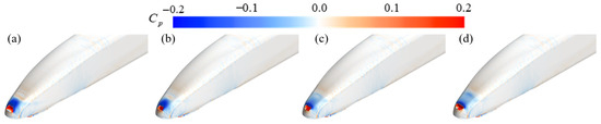
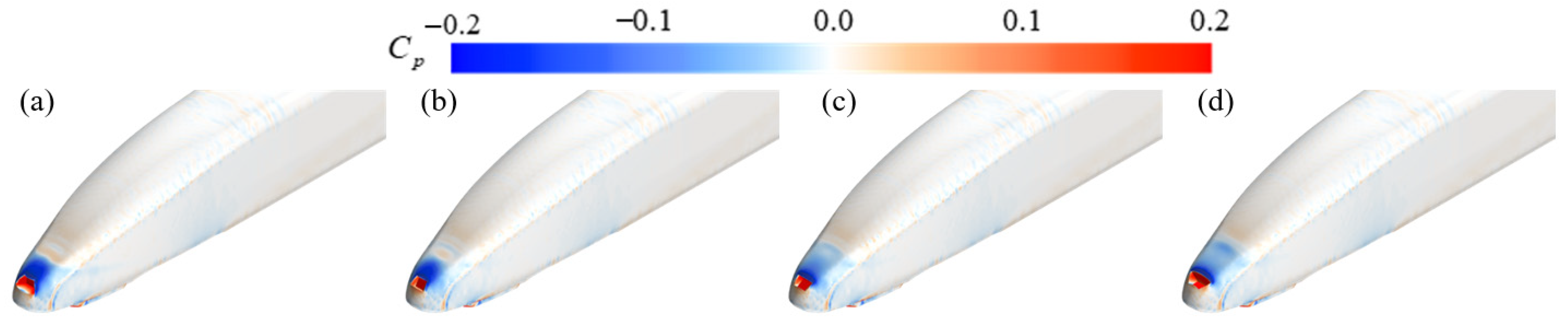
To better elucidate the impact on pressure distribution, Figure 24 compares the pressure-difference contours on the head-car surface under different jet angles. The pressure difference is defined by subtracting the baseline pressure from the controlled-case pressure. As the jet angle decreases, the negative-pressure-difference region becomes smaller. Notably, the jet in case A1 directly opposes the incoming free-stream flow, which induces a highly localized positive pressure near the jet nozzle due to intense flow stagnation. As illustrated in the pressure difference contours, the extent of the positive pressure difference zone (the orange-red region) in A1 is larger than that in A2. This aerodynamic phenomenon further explains why case A2 achieves the maximum pressure drag reduction rate for the head car.

Figure 24. Pressure-difference contours on the head-car surface under different sweeping-jet angles: (a) A1; (b) A2; (c) A3 and (d) A4.

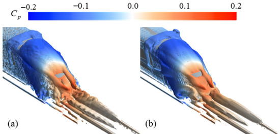
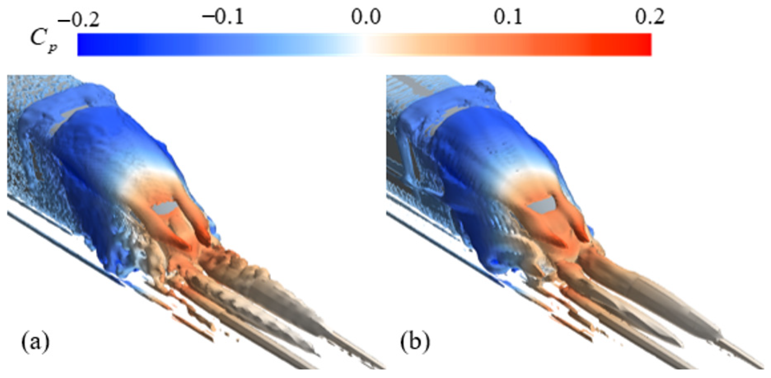
To gain a deeper interpretation of the altered wake structures, the downstream flow fields of the baseline and case A2 were compared. Case A2 was specifically selected as it represents a typical scenario exhibiting a severe tail-car drag penalty. Figure 25 compares the three-dimensional trailing vortical structures visualized using the Q-criterion isosurface. Visually, the trailing vortices in case A2 (Figure 25b) maintain a coherent tubular topology but appear noticeably more compressed and elongated compared to the baseline (Figure 25a). To quantify this structural alteration, data extracted at the x/H = 1.0 downstream cross-section reveals that while the total momentum-deficit area (U_x < 0.9U_∞) slightly decreases from 0.268% (baseline) to 0.258% (case A2), the minimum streamwise velocity within the vortex cores drops significantly from 52.47 m/s to 50.93 m/s.

Figure 25. Comparison of the time-averaged three-dimensional trailing vortical structures (visualized by the Q-criterion isosurface) between (a) the baseline and (b) case A2.

This quantitative evidence demonstrates that the severe drag penalty in case A2 is not caused by a macroscopic lateral expansion of the wake, but rather by vortex core intensification. The trailing vortices become structurally more energetic and tightly concentrated, which induces a much stronger localized suction effect (lower base pressure) over the rear surfaces of the tail car. This mechanism provides an explanation for the maximum drag penalty observed in this specific actuation scenario.

3.5. Effects of Sweeping-Jet Velocity

The sweeping-jet velocity also affects the aerodynamic drag and the flow structure around the train. Six jet velocities were considered. The bulk velocity U_bulk was increased from 10 m/s to 35 m/s with an interval of 5 m/s. The nondimensional velocities were 0.10U_∞ (V1), 0.15U_∞ (V2), 0.20U_∞ (V3), 0.25U_∞ (V4), 0.30U_∞ (V5), and 0.35U_∞ (V6). The baseline case without control was named V0. The six cases used the same model size, position, and jet angle.

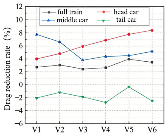
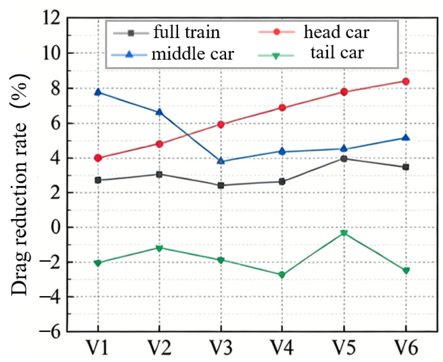
Figure 26 shows the drag-reduction rate of the train under different sweeping-jet velocities. All six jet velocities reduce the total aerodynamic drag of the three-car train. However, the total drag-reduction rates are close to each other, showing that jet velocity has a relatively small influence on the total drag reduction. For the head car, the drag-reduction rate increases with the jet velocity. When the jet velocity is V6, the head-car drag reduction reaches about 8.36%. For the middle car, the drag-reduction rate first decreases and then increases. The minimum value appears in V3, about 3.79%. The tail car experiences varying degrees of drag increase across the configurations; however, configuration V5 induces the minimum drag penalty, exhibiting an increase of only 0.31%. Considering the cumulative drag of the three cars, V5 yields the optimal overall drag-reduction performance among the six evaluated velocities.

Figure 26. Drag-reduction rate of the high-speed train under different sweeping-jet velocities.

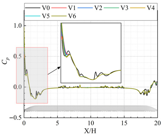
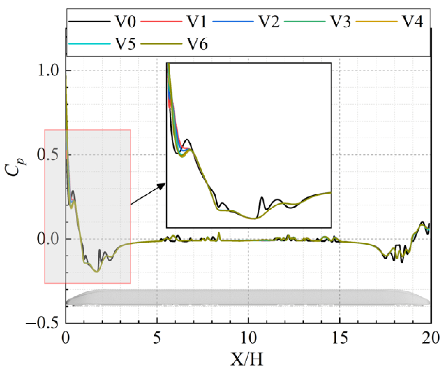
Figure 27 compares the pressure-coefficient curves along the center longitudinal section of the train under different jet velocities. Overall, the effect of jet velocity on the surface pressure coefficient along this section is small. In the enlarged region, the pressure coefficient on the head car decreases gradually as the jet velocity increases. However, the magnitude of this reduction attenuates at higher velocities. The curves for V4, V5, and V6 almost overlap. This shows that the control effect becomes nearly saturated when the jet velocity is higher than 0.25U_∞.

Figure 27. Pressure-coefficient curves along the center longitudinal section under different sweeping-jet velocities.

The non-monotonic variation in the tail-car drag with jet velocity suggests a balance between the local drag-reduction benefit and the downstream disturbance penalty. Increasing the jet velocity enhances the low-speed recirculation region near the nose and further reduces the head-car pressure drag. However, once the pressure-control effect becomes saturated, additional jet momentum does not produce a proportional reduction in head-car pressure. Instead, excessive momentum injection can strengthen the three-dimensional disturbance and alter the momentum distribution convected toward the tail car. This may intensify the wake deficit or reduce the pressure recovery capability of the streamlined tail, leading to a larger tail-car drag penalty. Therefore, V5 provides the best overall performance because it achieves sufficient head-car pressure control while maintaining a relatively small adverse effect on the tail car.

3.6. Energy Efficiency Assessment and Engineering Limitations

Based on the formulations defined in Section 2.8, Table 6 quantitatively addresses this by comparing the jet-flow power coefficient (C_P,j,flow) with the gross aerodynamic drag reduction coefficient (ΔC_D).

Table 6. Power accounting and ideal power-gain ratio evaluation for different sweeping-jet configurations.

Case No.	Velocity Ratio (Ubulk/U∞)	Area Ratio (Aj/S × 10−03)	Jet-Power Coefficient (CP,j,flow × 10−04)	Drag Reduction Coefficient (ΔCD)	Power-Gain Ratio (Gflow)
S1	0.25	1.48	1.63	0.0002	1.23
S2	0.25	3.30	3.86	0.0037	9.58
S3	0.25	6.39	6.72	0.0038	5.66
S4	0.25	9.16	11.4	0.0047	4.12
V1	0.10	9.16	5.48	0.0088	16.06
V2	0.15	9.16	8.55	0.0096	11.23
V3	0.20	9.16	12.0	0.0079	6.56
V4	0.25	9.16	15.5	0.0084	5.42
V5	0.30	9.16	18.4	0.0125	6.79
V6	0.35	9.16	22.6	0.0110	4.87

As indicated by the data, the mechanical power delivered to the external flow increases significantly at higher actuation intensities. Consequently, for the varying velocity cases (V1–V6), the power-gain ratio (G_flow) decreases from a maximum of 16.06 (Case V1) to 4.87 (Case V6). This demonstrates that while Case V5 achieves the optimum gross drag reduction, it does not correspond to the most power-efficient operating condition. Similarly, among the size variations, Case S2 yields the highest G_flow of 9.58. Importantly, G_flow remains strictly greater than 1.0 across the optimal cases. Under the adopted idealized accounting, this supports the aerodynamic leverage of the stagnation-zone momentum injection strategy, showing that the gross aerodynamic power savings consistently exceed the theoretical jet-flow power requirement.

However, several limitations in the current baseline study must be objectively acknowledged. First, as explicitly defined in Section 2.8, the evaluated G_flow serves as an upper-bound aerodynamic indicator. The internal pressure losses within the fluidic oscillator and the real-world electrical power demands of the actuation supply system were not directly resolved. For future engineering applications, transitioning from this theoretical positive energy gain to a practical net electrical saving is a critical challenge that necessitates a comprehensive evaluation coupling the aerodynamic benefits with the actual compressor power.

Furthermore, actual high-speed train operations involve complex environmental challenges that warrant future investigation. Under crosswind conditions, the lateral wind component may interact with the spatially oscillating jet, potentially deflecting the fluidic layer asymmetrically. The robustness of the sweeping jet’s control authority will likely depend on the momentum ratio between the jet and the crossflow, necessitating further studies on adaptive jet velocities to counteract lateral disturbances.

Similarly, tunnel entry and exit involve transient pressure-wave processes that differ from the baseline open-air condition considered here. Because the nose-mounted sweeping jet changes the local flow around the streamlined head, it may affect the formation of the initial compression wave and the pressure-gradient development during tunnel entry. Its influence on pressure variation, aerodynamic loads, and vehicle airtightness should therefore be evaluated in future transient studies.

While these complex aspects fall beyond the scope of the current steady-state, open-air investigation, they represent essential, next steps to validate the engineering applicability and completeness of the proposed control strategy.

4. Conclusions

The present study investigated active aerodynamic drag reduction in a high-speed train using sweeping jets. The effects of jet outlet size, jet angle, and jet velocity were analyzed by IDDES. The main conclusions are as follows:

(1)

The outlet size of the sweeping-jet model exerts a significant impact on drag reduction. In general, a larger outlet size gives a better drag-reduction effect. When the ratio between the jet outlet width and the train width is 5:50, the total drag reduction in the three-car train reaches about 1.5%. The maximum middle-car drag reduction is 4.55%, while the tail car shows drag increase in most size cases. The larger outlet size increases the low-speed recirculation region and weakens the direct impact of the incoming flow on the train surface.

(2)

The jet angle has a relatively small influence on the total drag reduction in the three-car train, but it changes the drag distribution among the head, middle, and tail cars. Among the four tested angles, 120° gives the best overall drag-reduction effect. The total drag reduction is about 2.84%, and the middle-car drag reduction reaches 6.19%. The 90° case is the only angle case that reduces the tail-car drag. The angle mainly affects the control effect by changing the size and position of the pressure-difference region on the train surface.

(3)

The jet velocity has a strong influence on the head-car drag. The head-car drag-reduction rate increases with velocity and reaches about 8.36% when the jet velocity is 0.35 U_∞. However, when the velocity is higher than 0.25U_∞, the pressure-control effect tends to become saturated. Considering the total drag of the three-car train, the best velocity is 0.30U_∞, with a total drag reduction of about 4.0%. Under the idealized jet-power accounting adopted in this study, the calculated gross aerodynamic power saving is larger than the jet-exit power benchmark for all investigated velocity cases. However, this result does not establish positive net electrical power saving because the internal pressure losses and the efficiency of the complete supply system were not modeled.

(4)

The fundamental flow-control mechanism lies in the formation of a low-speed recirculation zone immediately downstream of the sweeping-jet outlet. This localized region deflects the oncoming flow to create a buffer layer near the train surface, thereby reducing the local positive pressure and, consequently, the overall pressure drag. However, the nose-mounted sweeping jet also changes the downstream boundary-layer development and the momentum distribution approaching the tail car. Quantitative analyses reveal that the tail-car drag penalty is not caused by a macroscopic lateral expansion of the wake, but driven by trailing vortex core intensification. The highly concentrated and energetic vortex cores induce a stronger localized suction effect over the tail car. Therefore, the total drag-reduction performance depends on the balance between the drag reduction in the head/middle cars and the possible pressure-drag increase in the tail car.

As an initial exploratory framework, this study shows the aerodynamic potential of SWJ on high-speed trains. Building upon these mechanistic insights, future investigations will expand the parameter space and optimize the spatial arrangement of oscillators. It should be noted that the net electrical power saving was not directly evaluated here due to the omission of internal supply system losses. Therefore, assessing the actual system efficiency and pursuing a positive net energy saving under realistic operational conditions constitute the primary targets for upcoming engineering studies.

References

- Zhang, N.N.; Xu, Y.L. Study on the impact of high-speed railway on regional development along the line. Areal Res. Dev. 2005, 24, 32–36. (In Chinese) [Google Scholar]
- Li, S.W. Development trends of high-speed railway in the world. Railw. Tech. Superv. 2007, 35, 35–37. (In Chinese) [Google Scholar] [CrossRef] [Scilit]
- Wang, S.H. Development of high-speed railway in China and its economic impact. J. Southwest Jiaotong Univ. (Soc. Sci.) 2010, 11, 65–69. (In Chinese) [Google Scholar]
- Pan, Y.C. Numerical Study on Boundary Layer and Wake Flow of High-Speed Trains. Ph.D. Thesis, China Academy of Railway Sciences, Beijing, China, 2018. (In Chinese) [Google Scholar]
- Liang, X.F.; Tian, H.Q.; Zou, J.J. Wind-tunnel test and numerical simulation of longitudinal aerodynamic force of a power car. J. Natl. Univ. Def. Technol. 2003, 25, 101–105. (In Chinese) [Google Scholar]
- Yao, S.B.; Guo, D.L.; Yang, G.W.; Li, M.G. Distribution characteristics of aerodynamic drag of high-speed trains. J. China Railw. Soc. 2012, 34, 18–23. (In Chinese) [Google Scholar]
- Zhang, L.; Zhang, J.Y.; Li, T.; Zhang, Y.D. Multi-objective aerodynamic optimization design of high-speed train head shape. J. Southwest Jiaotong Univ. 2016, 51, 1055–1063. (In Chinese) [Google Scholar]
- Zhu, H.; Zhang, Y.; Zhao, H.; Wu, P.; Shao, X. Drag reduction technology of high-speed trains based on boundary-layer control. J. Traffic Transp. Eng. 2017, 17, 64–72. (In Chinese) [Google Scholar]
- Muñoz-Paniagua, J.; García, J. Aerodynamic drag optimization of a high speed train. J. Wind Eng. Ind. Aerodyn. 2020, 204, 104215. [Google Scholar] [CrossRef] [Scilit]
- Zhang, J. Wind-tunnel experimental study on the head shape of high-speed train EMU. Exp. Meas. Fluid Mech. 1997, 2, 85–89. (In Chinese) [Google Scholar]
- Zhang, Z.Z.; Zhou, D. Wind-tunnel experimental study on aerodynamic performance of high-speed trains with different head shapes. J. Cent. South Univ. (Sci. Technol.) 2013, 44, 2603–2608. (In Chinese) [Google Scholar] [CrossRef] [Scilit]
- Chen, B.Z.; Zhai, J.J. Optimization of high-speed train head shape. J. Dalian Jiaotong Univ. 2012, 33, 16–20. (In Chinese) [Google Scholar]
- Zhang, L.; Dai, Z.Y.; Li, T.; Zhang, J.Y. Multi-objective aerodynamic shape optimization of a streamlined high-speed train using kriging model. J. Zhejiang Univ.-Sci. A 2022, 23, 225–242. [Google Scholar] [CrossRef] [Scilit]
- Joslin, R.D. Aircraft laminar flow control. Annu. Rev. Fluid Mech. 1998, 30, 1–29. [Google Scholar] [CrossRef] [Scilit]
- Cattafesta, L.N.; Sheplak, M. Actuators for active flow control. Annu. Rev. Fluid Mech. 2011, 43, 247–272. [Google Scholar] [CrossRef] [Scilit]
- Glezer, A.; Amitay, M. Synthetic jets. Annu. Rev. Fluid Mech. 2002, 34, 503–529. [Google Scholar] [CrossRef] [Scilit]
- Smith, B.L.; Glezer, A. The formation and evolution of synthetic jets. Phys. Fluids 1998, 10, 2281–2297. [Google Scholar] [CrossRef] [Scilit]
- Greenblatt, D.; Wygnanski, I.J. The control of flow separation by periodic excitation. Prog. Aerosp. Sci. 2000, 36, 489–545. [Google Scholar] [CrossRef] [Scilit]
- Khan, T.I.; Tajik, A.R.; Parezanovic, V. Drag reduction of a generic transport vehicle model using a fluidic oscillator. Int. J. Thermofluids 2022, 15, 100180. [Google Scholar] [CrossRef] [Scilit]
- Cerretelli, C.; Kirtley, K. Boundary layer separation control with fluidic oscillators. J. Turbomach. 2009, 131, 041001. [Google Scholar] [CrossRef] [Scilit]
- Seifert, A.; Stalnov, O.; Sperber, D.; Arwatz, G.; Palei, V.; David, S.; Dayan, I.; Fono, I. Large trucks drag reduction using active flow control. In Proceedings of the 46th AIAA Aerospace Sciences Meeting and Exhibit, Honolulu, HI, USA, 7–10 January 2008. [Google Scholar]
- Seele, R.; Tewes, P.; Woszidlo, R.; McVeigh, M.A.; Lucas, N.J.; Wygnanski, I.J. Discrete sweeping jets as tools for improving the performance of the V-22. J. Aircr. 2009, 46, 2098–2106. [Google Scholar] [CrossRef] [Scilit]
- Woszidlo, R.; Ostermann, F.; Schmidt, H.J. Fundamental properties of fluidic oscillators for flow control applications. AIAA J. 2019, 57, 978–992. [Google Scholar] [CrossRef] [Scilit]
- Chen, X.; Zhong, S.; Ozer, O.; Weightman, A. Control of afterbody vortices from a slanted-base cylinder using sweeping jets. Phys. Fluids 2022, 34, 075115. [Google Scholar] [CrossRef] [Scilit]
- Chen, X.; Zhong, S.; Ozer, O.; Weightman, A. Drag reduction of a slanted-base cylinder using sweeping jets. Phys. Fluids 2022, 34, 105101. [Google Scholar] [CrossRef] [Scilit]
- Zhang, L.; Yang, M.; Liang, X. Experimental study on the effect of wind angles on pressure distribution of train streamlined zone and train aerodynamic forces. J. Wind Eng. Ind. Aerodyn. 2018, 174, 330–343. [Google Scholar] [CrossRef] [Scilit]
Disclaimer/Publisher’s Note: The statements, opinions and data contained in all publications are solely those of the individual author(s) and contributor(s) and not of MDPI and/or the editor(s). MDPI and/or the editor(s) disclaim responsibility for any injury to people or property resulting from any ideas, methods, instructions or products referred to in the content. |
© 2026 by the authors. Licensee MDPI, Basel, Switzerland. This article is an open access article distributed under the terms and conditions of the Creative Commons Attribution (CC BY) license.