Mathematical Modeling of Fluid Flow and Heat Transfer in the Laminar Entrance Region of a Cylindrical Pipe

Abstract

This study conducted a numerical simulation of laminar flow within a cylindrical pipe using a semi-implicit method. The full Navier–Stokes equations in cylindrical coordinates were solved, with modifications to the SIMPLE algorithm to handle pressure-linked equations. We evaluated three key thermophysical parameters—dynamic viscosity, specific heat capacity, and thermal conductivity—under both constant and variable conditions in the entrance region. Due to the process’s two-dimensional, time-dependent nature, third-kind boundary conditions were used to accurately model the effects of ambient temperature, external wind, and the pipe’s geometric and physical features. From the numerical results, we analyzed the velocity field, pressure distribution, surface friction coefficient, and temperature distribution at various pipe cross-sections. These findings are of practical and scientific importance: they offer insights into the hydrodynamics and thermal behavior of the internal flow and enhance understanding of fluid flow and heat transfer, improving predictive models. This advancement supports better design and operational control in pipeline systems.

1. Introduction

In the context of laminar flow through pipes, internal flow in cylindrical pipes is a critical aspect of energy engineering, chemical and oil/gas production, thermal systems, and the design and development of products using these systems. Analyzing the flow fields within cylindrical pipe systems helps clarify the mechanisms that generate velocity profiles, pressure fields, and temperature distributions across various cross-sections of the pipe system, ultimately enabling the quantification and improvement of the performance or efficiency of an entire engineering system by controlling the rate of heat transfer. Of particular importance is the entrance region of cylindrical pipes’ fluid flow, which is among the most complex regions from the perspective of hydrodynamic and thermal processes because the velocity and temperature profiles develop within this region; thus, investigating this area is essential from both theoretical and practical perspectives to evaluate the causes of energy loss (i.e., hydraulic loss, a drop in pressure, surface friction and heat transfer rate).

The study of fluid flow and heat transfer in channels has a rich history, beginning with the foundational analytical solutions for classical heat conduction and internal flows established by Graetz [1] and Nusselt [2]. The broader theoretical framework for hydrodynamics at low Reynolds numbers [3] and the application of dimensionality theory in chemical engineering [4] further solidified the basis for subsequent mathematical modeling of fluid behaviors.

Over time, researchers have expanded these fundamental concepts to analyze laminar flows in various complex geometries. For instance, the temperature fields and kinematic structures in semi-infinite prismatic channels of triangular [5], rectangular, and elliptical [6] cross-sections have been extensively studied. Furthermore, robust numerical algorithms have been developed to model specific geometric and physical phenomena, such as pulsating laminar flows in rectangular channels [7], suspension flows in flat channels [8], and fluid flow within eccentric annular domains [9].

The complexity of flow structures has also been a major focus, with investigations into the kinematic properties of swirling flows [10] and the mathematical modeling of two-phase fluid motion in concentrically located communicating pipes [11]. To simplify practical engineering applications, new predictive formulas for calculating the characteristics of liquid and gas flows in standard circular pipes have been successfully introduced [12].

In the field of thermal management, research increasingly focuses on improving heat transfer efficiency and predicting thermal distribution. Numerous studies have explored axial heat conduction in laminar duct flows [13] and designed advanced micro-channels optimized for high heat flux situations [14]. Recently, there has been a rise in using sophisticated numerical methods to analyze large-scale and specialized pipeline networks. Notable simulations include flow dynamics and heat transfer in relief pipelines of different diameters [15], the analysis of modern heat exchangers connected to two-pipe heating systems [16], and the complex flow behaviors within intricate gas network pipes [17]. Overall, these studies show a transition from traditional analytical approaches to advanced computational models capable of capturing both local thermal–hydraulic phenomena and overall fluid dynamics.

Regardless of these developments, current models either rely on low-order approximations, are configured for a particular geometry, or require substantial computation to make accurate predictions. This paper presents the design of a new model that integrates analysis and numerical methods to provide a versatile, high-precision formulation of laminar flow in cylindrical channels with arbitrary boundary conditions. This method contrasts with previous ones; unlike previous studies, it provides simultaneous, high-resolution velocity and temperature profiles in both the radial and axial directions while remaining computationally efficient. It also accounts for convective and diffusive processes, allowing the prediction of fluid flow and heat transfer performance over a very broad range of Reynolds, Prandtl, and Peclet numbers. This method is useful for enhancing the accuracy and applicability of laminar flow modeling and is also an effective engineering optimization tool that produces solutions between simplified analytical simulations and full numerical CFD models.

2. Materials and Methods

2.1. Mathematical Model

The mathematical model of the problem is formulated in cylindrical coordinates, taking into account the domain’s axial symmetry (Figure 1).

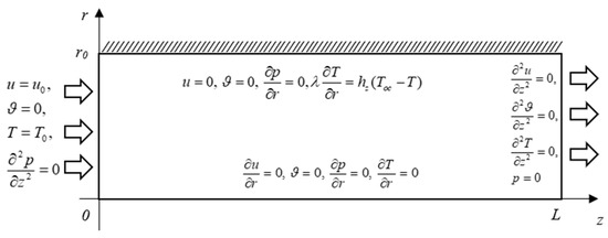
Figure 1. Geometry and boundary conditions of the problem.

We establish a longitudinal coordinate along the flow axis, $z$, measured from the inlet cross-section. For our specific simulation model incorporating a pipeline with an internal diameter of 100 mm, we select a section length $L$ (specifically, $L=300r_0$) that is significantly greater than the internal radius $r_0$ of the pipeline.

The radius $r_0$ serves as the upper limit for the radial coordinate $r$, which is measured outward from the flow axis.

At the entrance of the section, the longitudinal velocity is $u\left(0,r\right) = u_0,$ and the radial velocity is zero, $\vartheta (0,r)=0$. The entrance temperature is defined as $T(0,r)=T_0$.

On the flow axis $\left(r = 0\right)$, the conditions for axial symmetry are formulated as follows:

$${\displaystyle \frac{\partial u(z,0)}{\partial r}}=0, \hspace{0.33em}\hspace{0.33em}\hspace{0.33em} \vartheta (z,0)=0, \hspace{0.33em}\hspace{0.33em}\hspace{0.33em} {\displaystyle \frac{\partial T(z,0)}{\partial r}}=0.\hspace{0.33em}\hspace{0.33em}\hspace{0.33em}$$

(1)

At the channel wall, the fluid velocity becomes zero, but heat transfer still occurs:

$$u(z,r_0)=\vartheta (z,r_0)=0,\hspace{0.33em}\hspace{0.33em}\hspace{0.33em} \lambda {\displaystyle \frac{\partial T}{\partial r}}=h_z(T_{oc}-T(r_0)).\hspace{0.33em}\hspace{0.33em}\hspace{0.33em}$$

(2)

Here, $\lambda$ represents the thermal conductivity of the liquid, and $T_{oc}$ represents the outside temperature. The heat transfer coefficient $h_z$ is determined by accounting for the heat transfer from the liquid at the radial boundary $r = r_0 \left(d = 2r_0\right)$ into the wall material, the heat conduction through the wall material, and the convective heat transfer from the wall to the surrounding environment:

$${(h_z)}_{eff}={\displaystyle \frac{2\pi }{\frac{1}{r_0{h}_0}+\frac{\ln \left[\left(r_0+\delta \right)/r_0\right]}{{\lambda }_s}+\frac{1}{\left(r_0+\delta \right)h_1}}}.$$

(3)

Here $\delta$ is the pipeline wall thickness, and ${\lambda }_s$ is the thermal conductivity coefficient of the pipeline material.

The Graetz–Nusselt problem allows us to express the internal processes of the pipe, the pipe material and parameters, and the properties of the surrounding environment through a single, unified parameter. For this reason, this specific approach was selected over other formulas.

To calculate the value of the heat transfer coefficient from the liquid to the wall, the following formula was used:

$$h_0=N{u}_{\mathrm{int}}{\displaystyle \frac{\lambda }{2r_0}}.$$

(4)

Here the internal number $N{u}_0$ is calculated using the Graetz–Nusselt formula [7,8,9,10]:

$$\begin{array}{c}N{u}_{\mathrm{int}}=3.66+{\displaystyle \frac{0.0668\hspace{0.17em}\hspace{0.17em}(2r_0/x)\mathrm{Re}\mathrm{Pr}}{1+0.04\hspace{0.17em}\hspace{0.17em}{((2r_0/x)\mathrm{Re}\mathrm{Pr})}^{2/3}}}\hspace{0.17em}\hspace{0.17em}\hspace{0.17em},\hspace{0.17em}\hspace{0.17em}\hspace{0.17em}{T}_{oc}=const\hspace{0.17em},\hspace{0.17em}\hspace{0.17em}\hspace{0.17em}\hspace{0.17em}\mathrm{Pr}\ge 5.\\ N{u}_{\mathrm{int}}={\displaystyle \frac{\frac{3.66}{\tanh [2.264G{z}_D^{-1/3}+1.7G{z}_D^{-2/3}]}+0.0499G{z}_D\tanh (G{z}_D^{-1})}{\tanh \left(2.432{\mathrm{Pr}}^{1/6}G{z}_D^{-1/6}\right)}},\hspace{0.17em}\hspace{0.17em}\hspace{0.17em}\hspace{0.17em}\hspace{0.17em}0.1\le \mathrm{Pr}<5\\ \mathrm{Here} G{z}_D=\left(D/x\right)\mathrm{Re}\mathrm{Pr}\end{array}$$

(5)

It is designed for a laminar flow of liquid at a constant ambient temperature and for Prandtl number values of $Pr\ge 5$. Here $x$ is the length of the initial section;

$$\mathrm{Re}={\displaystyle \frac{2r_0{u}_0}{v}}$$

(6)

is the Reynolds criterion (number) for fluid flow; $v$ is the kinematic viscosity of the fluid;

$$\mathrm{Pr}={\displaystyle \frac{c_{\vartheta }v\rho }{\lambda }}$$

(7)

is the Prandtl criterion of liquid; $c_{\vartheta }$ is the specific heat capacity and $\rho$ is the density of the liquid, which are taken as constant values.

The values of the heat transfer coefficient from the pipeline walls to the environment were calculated using the following formula:

$$h_1=N{u}_{ext}{\displaystyle \frac{{\lambda }_{aer}}{2\left(r_0+\delta \right)}}.$$

(8)

Here the external Nusselt number was determined according to the formula [7,8,9,10]:

$$N{u}_{ext}=0.3+{\displaystyle \frac{0.62\sqrt{{\mathrm{Re}}_{aer}}{\mathrm{Pr}}_{aer}^{1/3}}{{\left[1+{(0.4/{\mathrm{Pr}}_{aer})}^{2/3}\right]}^{1/4}}}{\left[1+{({\mathrm{Re}}_{aer}/282000)}^{5/8}\right]}^{4/5}\hspace{0.17em}\hspace{0.17em}$$

(9)

Here the Reynolds criterion for the environment is calculated as

$${\mathrm{Re}}_{aer}={\displaystyle \frac{2\left(r_0+\delta \right)u_{aer}}{v_{aer}}}.$$

(10)

The external Nusselt formula, according to [1], is reliable for intervals $0.7\le {\mathrm{Pr}}_{aer}\le 500\hspace{0.17em},\hspace{0.17em}\hspace{0.17em}1\hspace{0.17em}\hspace{0.17em}\le {\mathrm{Re}}_{aer}\hspace{0.17em}\hspace{0.17em}\le {10}^6$.

Here, $R{e}_{aer}\hspace{0.17em}\hspace{0.17em}\mathrm{and}\hspace{0.17em}\hspace{0.17em}{\mathrm{Pr}}_{aer}$ are the Reynolds and Prandtl numbers for the surrounding air.

At the outlet section of the channel, smooth conjugation conditions were used:

$${\displaystyle \frac{{\partial }^{2}u(L,r)}{\partial z^2}}={\displaystyle \frac{{\partial }^2\vartheta (L,r)}{\partial z^2}}=0.$$

(11)

The inclusion of pressure in the equations of conservation of momentum in the longitudinal and radial directions, expressed as first derivatives with respect to coordinates, requires the formulation of conditions for pressure with respect to coordinates. These were

$${\displaystyle \frac{\partial p(x,0)}{\partial r}}=0,\hspace{0.17em}\hspace{0.17em}\hspace{0.17em}p(L,r)=0.$$

(12)

Here, the first condition reflects the symmetry of the flow relative to the flow axis, while the second condition is determined by the flow exiting into the atmosphere. Accordingly, this condition reflects zero excess fluid pressure at the atmospheric exit.

When implementing the SIMPLE method, an elliptic equation is first solved for pressure, followed by a parabolic equation. This means that additional boundary conditions are required for the pressure along the longitudinal and radial coordinates. These conditions include the wall condition,

$${\displaystyle \frac{\partial p(x,r_0)}{\partial r}}=0,$$

(13)

which follows from the equation for conservation of momentum along the radial coordinate and the condition at the channel entrance,

$${\displaystyle \frac{\partial p^2(0,r)}{\partial z^2}}=0,$$

(14)

which corresponds to a smooth continuation of the pressure conjugation at the inlet.

The problem was solved using the equations of conservation of mass, momentum in two coordinates, and energy:

$$\left\{\begin{array}{l}{\displaystyle \frac{1}{r}}{\displaystyle \frac{\partial \left(r{u}_r\right)}{\partial r}}+{\displaystyle \frac{\partial u_z}{\partial z}}=0,\\ \rho \left({\displaystyle \frac{\partial u_z}{\partial t}}+u_r{\displaystyle \frac{\partial u_z}{\partial r}}+u_z{\displaystyle \frac{\partial u_z}{\partial z}}\right)=-{\displaystyle \frac{\partial p}{\partial z}}+\left({\displaystyle \frac{1}{r}}{\displaystyle \frac{\partial }{\partial r}}\left(\mu (T)r{\displaystyle \frac{\partial u_z}{\partial r}}\right)+{\displaystyle \frac{\partial }{\partial z}}\left(\mu (T){\displaystyle \frac{\partial u_z}{\partial z}}\right)\right),\\ \rho \left({\displaystyle \frac{\partial u_r}{\partial t}}+u_r{\displaystyle \frac{\partial u_r}{\partial r}}+u_z{\displaystyle \frac{\partial u_r}{\partial z}}\right)=-{\displaystyle \frac{\partial p}{\partial r}}+\left({\displaystyle \frac{1}{r}}{\displaystyle \frac{\partial }{\partial r}}\left(\mu (T)r{\displaystyle \frac{\partial u_r}{\partial r}}\right)+{\displaystyle \frac{\partial }{\partial z}}\left(\mu (T){\displaystyle \frac{\partial u_r}{\partial z}}\right)-\mu (T){\displaystyle \frac{u_r}{r^2}}\right),\\ \rho c_v\left(T\right)\left({\displaystyle \frac{\partial T}{\partial t}}+u_r{\displaystyle \frac{\partial T}{\partial r}}+u_z{\displaystyle \frac{\partial T}{\partial z}}\right)=\left({\displaystyle \frac{1}{r}}{\displaystyle \frac{\partial }{\partial r}}\left(\lambda (T)r{\displaystyle \frac{\partial T}{\partial r}}\right)+{\displaystyle \frac{\partial }{\partial z}}\left(\lambda (T){\displaystyle \frac{\partial T}{\partial z}}\right)\right).\end{array}\right.$$

(15)

Here, $\mu (T)$ denotes the dynamic viscosity of the liquid, and $c_v(T)$ its specific heat capacity.

The system of equations, subject to the stated boundary conditions, was solved numerically using dimensionless variables. The pipeline radius $r_0$, the inlet flow velocity $u_0,$ and the inlet fluid temperature $T_0$ served as the scaling variables. Accordingly, the time scale was $r_0/u_0$ and the pressure scale $\rho u_0^2$.

Through these transformations, the model was extended to an infinite domain.

$$\overline{r}={\displaystyle \frac{r}{r_0}},\hspace{0.17em}\hspace{0.17em}\hspace{0.17em}\overline{z}={\displaystyle \frac{z}{r_0}},\hspace{0.17em}\hspace{0.17em}\hspace{0.17em}\overline{u_r}={\displaystyle \frac{u_r}{u_0}},\hspace{0.17em}\hspace{0.17em}\hspace{0.17em}\hspace{0.17em}\overline{u_z}={\displaystyle \frac{u_z}{u_0}},\hspace{0.17em}\hspace{0.17em}\hspace{0.17em}\overline{t}={\displaystyle \frac{t{u}_0}{r_0}},\hspace{0.17em}\hspace{0.17em}\mathrm{Re}={\displaystyle \frac{\rho u_0{r}_0}{\mu }},\hspace{0.17em}\hspace{0.17em}\overline{p}={\displaystyle \frac{p}{\rho u_0^2}};$$

Consequently, the complete system of Navier–Stokes equations in dimensionless variables takes the following form:

$$\left\{\begin{array}{l}{\displaystyle \frac{1}{\overline{r}}}{\displaystyle \frac{\partial \left(r\overline{\vartheta }\right)}{\partial \overline{r}}}+{\displaystyle \frac{\partial \overline{u}}{\partial \overline{z}}}=0,\\ {\displaystyle \frac{\partial \overline{u}}{\partial \overline{t}}}+\overline{\vartheta }{\displaystyle \frac{\partial \overline{u}}{\partial \overline{r}}}+\overline{u}{\displaystyle \frac{\partial \overline{u}}{\partial \overline{z}}}=-{\displaystyle \frac{\partial \overline{p}}{\partial \overline{z}}}+{\displaystyle \frac{1}{\mathrm{Re}}}\left({\displaystyle \frac{1}{\overline{r}}}{\displaystyle \frac{\partial }{\partial \overline{r}}}\left(\overline{\mu }\overline{r}{\displaystyle \frac{\partial \overline{u}}{\partial \overline{r}}}\right)+{\displaystyle \frac{\partial }{\partial \overline{z}}}\left(\overline{\mu }{\displaystyle \frac{\partial \overline{u}}{\partial \overline{z}}}\right)\right),\\ {\displaystyle \frac{\partial \overline{\vartheta }}{\partial \overline{t}}}+\overline{\vartheta }{\displaystyle \frac{\partial \overline{\vartheta }}{\partial \overline{r}}}+\overline{u}{\displaystyle \frac{\partial \overline{\vartheta }}{\partial \overline{z}}}=-{\displaystyle \frac{\partial \overline{p}}{\partial \overline{r}}}+{\displaystyle \frac{1}{\mathrm{Re}}}\left({\displaystyle \frac{1}{\overline{r}}}{\displaystyle \frac{\partial }{\partial \overline{r}}}\left(\overline{r}\overline{\mu }{\displaystyle \frac{\partial \overline{\vartheta }}{\partial \overline{r}}}\right)+{\displaystyle \frac{\partial }{\partial \overline{z}}}\left(\overline{\mu }{\displaystyle \frac{\partial \overline{\vartheta }}{\partial \overline{z}}}\right)-\overline{\mu }{\displaystyle \frac{\overline{\vartheta }}{{\overline{r}}^2}}\right),\\ \left({\displaystyle \frac{\partial \overline{T}}{\partial \overline{t}}}+\overline{\vartheta }{\displaystyle \frac{\partial \overline{T}}{\partial \overline{r}}}+\overline{u}{\displaystyle \frac{\partial \overline{T}}{\partial \overline{z}}}\right)={\displaystyle \frac{1}{\overline{r}}}{\displaystyle \frac{\partial }{\partial \overline{r}}}\left(\overline{r}{\displaystyle \frac{1}{\mathrm{Re}\hspace{0.17em}\mathrm{Pr}(T)}}\overline{\mu }{\displaystyle \frac{\partial \overline{T}}{\partial \overline{r}}}\right)+{\displaystyle \frac{\partial }{\partial \overline{z}}}\left({\displaystyle \frac{1}{\mathrm{Re}\hspace{0.17em}\mathrm{Pr}(T)}}\overline{\mu }{\displaystyle \frac{\partial \overline{T}}{\partial \overline{z}}}\right)\end{array}\right.$$

(16)

Here

$$\mathrm{Pr}(T)={\displaystyle \frac{\mu \left(T\right)C_v\left(T\right)}{\lambda (T)}}, \overline{\mu }={\displaystyle \frac{\mu \left(T\right)}{\mu }}$$

(17)

$$\mu \left(T\right)=2.414\times {10}^{{\displaystyle \frac{247.8}{T-140}}-5},\hspace{0.17em}\hspace{0.17em}\hspace{0.17em}\hspace{0.17em}\hspace{0.17em}{c}_v\left(T\right)=4180+3.1(T-20),\hspace{0.17em}\hspace{0.17em}\hspace{0.17em}\hspace{0.17em}\lambda \left(T\right)=0.561+0.0019T.$$

(18)

2.2. Numerical Method for Solving the System of Dimensionless Full Navier–Stokes Equations on the Initial Section of a Cylindrical Channel

To solve the problem, the following discretisation parameters were selected. The number of equally spaced nodes along the dimensionless radial coordinate was $N_r+1=101$; the number of equally spaced nodes along the dimensionless longitudinal coordinate was $N_z+1=201$; and the total number of dimensionless time steps was $N_t=50000$.

The corresponding dimensionless step sizes were $\mathrm{\Delta }t=0.005,$ $\mathrm{\Delta }z=1/N_z,$ and $\mathrm{\Delta }r=1/N_r$. This choice ensures sufficient spatial mesh resolution in both the radial and axial directions, while the small time step guarantees the stability and accuracy of the numerical solution.

For validation purposes, the simulations in COMSOL Multiphysics were configured to match the grid of our program, utilizing a 100 × 200 domain dimension with its built-in “extra fine” mesh setting. Additionally, a time step of 0.005 was applied. The average computation time required to reach a steady-state solution was approximately 10–12 min for both our custom code and the commercial software packages.

The hydrodynamic problem was solved using the SIMPLE algorithm. For calculations at the new time step $n+1$, we first determine the intermediate values of the velocity components, ${\tilde{u}}_{i,j}$ and ${\tilde{\vartheta }}_{i,j}$, using the following equations:

$$\left\{\begin{array}{l}{\displaystyle \frac{\partial {\tilde{u}}_{i,j}^n}{\partial t}}+{\displaystyle \frac{\partial p_{i,j}^n}{\partial z}}={\phi }_u\left(\tilde{u},\tilde{\vartheta }\right),\\ {\displaystyle \frac{\partial {\tilde{\vartheta }}_{i,j}^n}{\partial t}}+{\displaystyle \frac{\partial p_{i,j}^n}{\partial r}}={\phi }_{\vartheta }\left(\tilde{u},\tilde{\vartheta }\right),\end{array}\right.$$

(19)

where

$$\begin{array}{l}{\phi }_u\left(u,\vartheta \right)={\displaystyle \frac{1}{\mathrm{Re}}}\left({\displaystyle \frac{1}{r}}{\displaystyle \frac{\partial }{\partial r}}\left(r{\displaystyle \frac{\partial u}{\partial r}}\right)+{\displaystyle \frac{{\partial }^{2}u}{\partial z^2}}\right)-\vartheta {\displaystyle \frac{\partial u}{\partial r}}-u{\displaystyle \frac{\partial u}{\partial z}},\\ {\phi }_{\vartheta }\left(u,\vartheta \right)={\displaystyle \frac{1}{\mathrm{Re}}}\left({\displaystyle \frac{1}{r}}{\displaystyle \frac{\partial }{\partial r}}\left(r{\displaystyle \frac{\partial \vartheta }{\partial r}}\right)+{\displaystyle \frac{{\partial }^2\vartheta }{\partial z^2}}\right)-\vartheta {\displaystyle \frac{\partial \vartheta }{\partial r}}-u{\displaystyle \frac{\partial \vartheta }{\partial z}}.\end{array}$$

(20)

New components of the pressure gradient were taken into account in the second part of the calculation.

$$\left\{\begin{array}{l}{\displaystyle \frac{\partial u_{i,j}^{n+1}}{\partial t}}+{\displaystyle \frac{\partial p_{i,j}^{n+1}}{\partial z}}={\phi }_u\left(\tilde{u},\tilde{\vartheta }\right),\\ {\displaystyle \frac{\partial {\vartheta }_{i,j}^{n+1}}{\partial t}}+{\displaystyle \frac{\partial p_{i,j}^{n+1}}{\partial r}}={\phi }_{\vartheta }\left(\tilde{u},\tilde{\vartheta }\right).\end{array}\right.$$

(21)

The right-hand sides of these equations were taken from the results of the previous calculation step. Zero coordinate velocities were assumed as the initial distributions, meaning the computation begins with the fluid at rest.

Term-by-term subtraction of the last two systems allows us to obtain the following dependencies:

$$\left\{\begin{array}{l}{\displaystyle \frac{u_{i,j}^{n+1}-{\tilde{u}}_{i,j}^n}{\mathrm{\Delta }t}}+{\displaystyle \frac{\partial \left(p_{i,j}^{n+1}-p_{i,j}^n\right)}{\partial z}}=0,\\ {\displaystyle \frac{{\vartheta }_{i,j}^{n+1}-{\tilde{\vartheta }}_{i,j}^n}{\mathrm{\Delta }t}}+{\displaystyle \frac{\partial \left(p_{i,j}^{n+1}-p_{i,j}^n\right)}{\partial r}}=0.\end{array}\right.$$

(22)

If we introduce a correction to the pressure $\delta p_{i,j}=p_{i,j}^{n+1}-p_{i,j}^n$, then from the last system we can compose an elliptic equation with respect to it:

$${\displaystyle \frac{1}{r}}{\displaystyle \frac{\partial }{\partial r}}\left(r{\displaystyle \frac{\partial \delta p_{i,j}}{\partial r}}\right)+{\displaystyle \frac{{\partial }^2\delta p_{i,j}}{\partial z^2}}=-{\displaystyle \frac{1}{\mathrm{\Delta }t}}\left({\displaystyle \frac{1}{r}}{\displaystyle \frac{\partial \left(r\tilde{\vartheta }\right)}{\partial r}}+{\displaystyle \frac{\partial \tilde{u}}{\partial z}}\right),$$

(23)

where the unconditional fulfillment of the equation of conservation of mass was taken into account

$${\displaystyle \frac{1}{r}}{\displaystyle \frac{\partial \left(r{\vartheta }^{n+1}\right)}{\partial r}}+{\displaystyle \frac{\partial u^{n+1}}{\partial z}}=0$$

(24)

at the $(n+1)$-th time step.

Thus, solving the hydrodynamic problem at the new time step n + 1 using the known values $u_{i,j}^n,{\vartheta }_{i,j}^n\hspace{0.17em}\mathrm{and}\hspace{0.17em}{p}_{i,j}^n$ proceeds in the following stages: The equations are solved for the intermediate velocity components ${\tilde{u}}_{i,j}^n$ and ${\tilde{\vartheta }}_{i,j}^n$; the equation is solved for the pressure increment $\delta p_{i,j}$; an adjustment is applied to the pressure field: $p_{i,j}^{n+1}=p_{i,j}^n+\delta p_{i,j}$; and corrections are made to the velocity components:

$$u_{i,j}^{n+1}={\tilde{u}}_{i,j}-\mathrm{\Delta }t{\displaystyle \frac{\partial \delta p_{i,j}}{\mathrm{\Delta }z}}, {\vartheta }_{i,j}^{n+1}={\tilde{\vartheta }}_{i,j}-\mathrm{\Delta }t{\displaystyle \frac{\partial \delta p_{i,j}}{\mathrm{\Delta }r}}.$$

(25)

Because the functions ${\phi }_u(\tilde{u},\tilde{\vartheta })$ and ${\phi }_{\vartheta }(\tilde{u},\tilde{\vartheta })$ are nonlinear, successive approximations are iterated until the process converges to a predetermined accuracy. Only then is the temperature field problem solved.

Let us examine the specific steps involved in solving the hydrodynamic problem.

To calculate the intermediate values of the longitudinal velocity for $0<i<N_z,$ a semi-explicit scheme was used:

$$\begin{array}{c}{\displaystyle \frac{{\tilde{u}}_{i,j}-u_{i,j}^n}{\mathrm{\Delta }t}}+{\vartheta }_{i,j}^n{\displaystyle \frac{u_{i,j}^n-u_{i,j-1}^n}{\mathrm{\Delta }r}}+u_{i,j}^n{\displaystyle \frac{u_{i,j}^n-u_{i-1,j}^n}{\mathrm{\Delta }z}}=\\ =-{\displaystyle \frac{p_{i,j}^n-p_{i,j-1}^n}{\mathrm{\Delta }z}}+{\displaystyle \frac{1}{\mathrm{Re}{r}_j}}{\displaystyle \frac{{\mu }_{i,j+1/2}{r}_{j+1/2}\hspace{0.17em}\hspace{0.17em}{\tilde{u}}_{i,j+1}-2r_j{\mu }_{i,}{\tilde{u}}_{i,j}+r_{j-1/2}{\mu }_{i,j-1/2}{\tilde{u}}_{i,j-1}}{\mathrm{\Delta }{r}^2}}+\\ +{\displaystyle \frac{1}{\mathrm{Re}}}{\displaystyle \frac{{\mu }_{i,j+1/2}{u}_{i+1,j}^n-2{\mu }_{i,j}{\tilde{u}}_{i,j}+{\mu }_{i,j-1/2}{u}_{i-1,j}^{n+1}}{\mathrm{\Delta }{z}^2}}\end{array}$$

(26)

in designations $r_j=j\mathrm{\Delta }r,\hspace{0.17em}\hspace{0.17em}{r}_{j\pm 1/2}\hspace{0.17em}=\left(j\pm 1/2\right)\mathrm{\Delta }r,$

$$\begin{array}{c}\begin{array}{c}{a}_j={\displaystyle \frac{{\mu }_{i,j+1/2}\mathrm{\Delta }t}{\mathrm{Re}\mathrm{\Delta }{r}^2}}\left(1+0.5/j\right),\hspace{0.17em}\hspace{0.17em}\hspace{0.17em}\hspace{0.17em}{c}_j={\displaystyle \frac{{\mu }_{i,j-1/2}\mathrm{\Delta }t}{\mathrm{Re}\mathrm{\Delta }{r}^2}}\left(1-0.5/j\right),\hspace{0.17em}\hspace{0.17em}\hspace{0.17em}\hspace{0.17em}\\ b_j=1+{\displaystyle \frac{2\mathrm{\Delta }t{\mu }_{i,j}}{\mathrm{Re}}}\left({\displaystyle \frac{1}{\mathrm{\Delta }{r}^2}}+{\displaystyle \frac{1}{\mathrm{\Delta }{z}^2}}\right),\end{array}\\ \begin{array}{c}{d}_j=-u_{i,j}^n+{\vartheta }_{i,j}^n\mathrm{\Delta }t{\displaystyle \frac{u_{i,j}^n-u_{i,j-1}^n}{\mathrm{\Delta }r}}+u_{i,j}^n\mathrm{\Delta }t{\displaystyle \frac{u_{i,j}^n-u_{i-1,j}^n}{\mathrm{\Delta }z}}+\\ +{\displaystyle \frac{p_{i,j}^n-p_{i-1,j}^n}{\mathrm{\Delta }z}}-{\displaystyle \frac{\mathrm{\Delta }t}{\mathrm{Re}\mathrm{\Delta }{z}^2}}\left({\mu }_{i,j+1/2}{u}_{i+1,j}^n+{\mu }_{i,j-1/2}{u}_{i-1,j}^{n+1}\right)\end{array}\end{array}$$

(27)

for a recurrent formula

$${\tilde{u}}_{i,j}^{n+1}={\alpha }_j{\tilde{u}}_{i,j+1}^{n+1}+{\beta }_j$$

(28)

we will receive

$${\alpha }_j={\displaystyle \frac{a_j}{b_j-c_j{\alpha }_{j-1}}}, {\beta }_j={\displaystyle \frac{c_j{\beta }_{j-1}-f_j}{b_j-c_j{\alpha }_{j-1}}}.$$

(29)

On the axis, they accepted ${\alpha }_0=1,$ ${\beta }_0=0$. The condition was used on the walls. ${\tilde{u}}_{i,Nr}=0.$ At the exit from the section (at $i=N_z$) the condition was used.

$${\tilde{u}}_{Nz,j}^{n+1}=2{\tilde{u}}_{Nz-1,j}^{n+1}-{\tilde{u}}_{Nz-2,j}^{n+1}$$

(30)

It was considered sufficient to use the Thomas algorithm only along the radial coordinate.

Similarly, we found the values ${\tilde{\vartheta }}_{i,j}$ taking into account the values of the coefficients

$$\begin{array}{c}{b}_j=1+{\displaystyle \frac{2\mathrm{\Delta }t{\mu }_{i,j}}{\mathrm{Re}}}\left({\displaystyle \frac{1}{\mathrm{\Delta }{r}^2}}+{\displaystyle \frac{1}{\mathrm{\Delta }{z}^2}}\right)+{\displaystyle \frac{\mathrm{\Delta }t\hspace{0.17em}{\vartheta }_{i,j}^n{\mu }_{i,j}}{\mathrm{Re}\hspace{0.17em}{j}^2\mathrm{\Delta }{r}^2}}\\ \begin{array}{c}{d}_j=-{\vartheta }_{i,j}^n+\mathrm{\Delta }t{\vartheta }_{i,j}^n{\displaystyle \frac{{\vartheta }_{i,j}^n-{\vartheta }_{i,j-1}^n}{\mathrm{\Delta }r}}+\mathrm{\Delta }t{u}_{i,j}^n{\displaystyle \frac{{\vartheta }_{i,j}^n-{\vartheta }_{i-1,j}^n}{\mathrm{\Delta }z}}+\\ +{\displaystyle \frac{p_{i,j}^n-p_{i-1,j}^n}{\mathrm{\Delta }r}}-{\displaystyle \frac{\mathrm{\Delta }t}{\mathrm{Re}\mathrm{\Delta }{z}^2}}\left({\mu }_{i+1/2,j}{\vartheta }_{i+1,j}^n+{\mu }_{i-1/2,j}{\vartheta }_{i-1,j}^{n+1}\right).\end{array}\end{array}$$

(31)

At the boundaries for the radial velocity, we took ${\alpha }_0=0,$${\beta }_0=0$, ${\tilde{\vartheta }}_{i,Nr}^n=0$ and ${\tilde{\vartheta }}_{Nz,j}^{n+1}=2{\tilde{\vartheta }}_{Nz-1,j}^{n+1}-{\tilde{\vartheta }}_{Nz-2,j}^{n+1}.$

The equations for the pressure increase were solved by the establishment method, for which a fictitious time was introduced $t_0$:

$${\displaystyle \frac{\partial \delta p}{\partial t_0}}={\displaystyle \frac{1}{r}}{\displaystyle \frac{\partial }{\partial r}}\left(r{\displaystyle \frac{\partial \delta p}{\partial r}}\right)+{\displaystyle \frac{{\partial }^2\delta p}{\partial z^2}}+{\displaystyle \frac{1}{\mathrm{\Delta }t}}\left({\displaystyle \frac{1}{r}}{\displaystyle \frac{\partial \left(r\tilde{\vartheta }\right)}{\partial r}}+{\displaystyle \frac{\partial \tilde{u}}{\partial z}}\right).$$

(32)

The integration step with respect to $t_0$ was set to ${\delta }_t=0.05$, and the superscript $k$ denotes the iteration index of the approximation. For the initial time step $\left(n = 1\right)$, the first approximation was set to $\delta p_{i,j}^0=0$. For subsequent time steps $\left(n > 1\right)$, the initial values $\delta p_{i,j}^0$ were taken from the previous time step’s results. During successive iterations, the condition $\delta p_{i,j}^{k+1}=0$ was enforced at the boundaries $\left(i = 0, i = N_z, j = 0 \hspace{0.17em}\hspace{0.17em}\mathrm{and}\hspace{0.17em}\hspace{0.17em} j = N_r\right)$.

The sweep process for pressure increment was organized along the radial coordinate. The diagonal advantage of the coefficients was enhanced by the central term of the second derivative with respect to z.

The calculations for k were repeated until the condition was met.

$${\max }_{\left(0<i<N_z\right)\times \left(0<j<N_r\right)}\left|\delta p_{i,j}^k-\delta p_{i,j}^{k+1}\right|<{\epsilon }_{\delta p}.$$

(33)

The pressure values at the calculated nodes in $n+1$ the -th time step were

$$p_{i,j}^{n+1}=p_{i,j}^n+\delta p_{i,j}^{k+1}$$

(34)

and the values of the components of the velocity vector were

$$u_{i,j}^{n+1}={\tilde{u}}_{i,j}-\mathrm{\Delta }t{\displaystyle \frac{\partial \delta p_{i,j}^{k+1}}{\mathrm{\Delta }z}}, {\vartheta }_{i,j}^{n+1}={\tilde{\vartheta }}_{i,j}-\mathrm{\Delta }t{\displaystyle \frac{\partial \delta p_{i,j}^{k+1}}{\mathrm{\Delta }r}}.$$

(35)

To determine the temperature field for $n+1$ the -th time step, a running process was organized as in the processes of finding ${\tilde{u}}_{i,j}$ and ${\tilde{\vartheta }}_{i,j}$.

The time calculations continued until $N_t=50000$ or when the largest deviations in the values of longitudinal and transverse velocities satisfied the following conditions:

$${\max }_{i\in \left(1,N_z\right)\times j\in \left(0,N_r-1\right)}\left|u_{i,j}^n-u_{i,j}^{n+1}\right|<{\epsilon }_u,\hspace{0.17em}\hspace{0.17em} {\max }_{i\in \left(1,N_z\right)\times j\in \left(1,N_r-1\right)}\left|{\vartheta }_{i,j}^n-{\vartheta }_{i,j}^{n+1}\right|<{\epsilon }_{\vartheta }.$$

(36)

3. Results

Figure 2 compares the longitudinal velocity profiles obtained using the developed method with the numerical results of the Comsol Multiphysics package. They relate to sections $\overline{x}=5$ (curves 1 and 2) and $\overline{x}=20$ (curve 3) and were obtained at Reynolds numbers $\mathrm{Re}=1200$ (curves 1 and 3) and $\mathrm{Re}=400$ (curve 3).

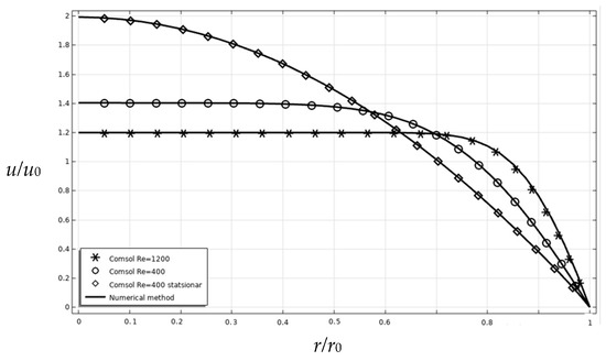
Figure 2. Comparison of the model results with Comsol Multiphysics simulations for axial velocity at various cross-sections.

To ensure consistency and full reproducibility, the numerical model was set up using the laminar flow and heat transfer in fluid physics interfaces within COMSOL Multiphysics. The model was configured with the exact same mesh parameters as the custom-developed software. The computational domain was discretized using a structured grid with 101 nodes along the radial axis and 201 nodes along the axial axis. Additionally, the time-stepping method utilized a constant time step of [0.005], and the iterative solver convergence criteria were defined with a step size of [10⁻⁶].

Comparison of the results obtained from the COMSOL simulations and the proposed numerical method. The discrete geometric markers represent the COMSOL data (diamonds: stationary Re = 400; circles: transient Re = 400; stars: Re = 1200). The solid continuous lines underlying the markers denote the results calculated using the proposed numerical method.

At the outlet section (diamonds), the axial velocity matches the classical quadratic Poiseuille profile well.

In the laminar regime, the hydraulic resistance coefficient is inversely proportional to the Reynolds number and is determined by the following expression:

$$f={\displaystyle \frac{64}{\mathrm{Re}}}$$

(37)

The friction coefficient used in the calculations is equal to

$$\tau ={\left.{\displaystyle \frac{f}{4}}\right|}_{r=r_0}$$

(38)

The wall shear stress in the pipeline is determined using the following formula:

$$\tau ={\left.\mu \left({\displaystyle \frac{\partial u}{\partial r}}\right)\right|}_{r=R}$$

(39)

In dimensionless form, this expression can be written in terms of the Reynolds number:

$$\tau ={\left.{\displaystyle \frac{2}{\mathrm{Re}}}\left({\displaystyle \frac{\partial u}{\partial r}}\right)\right|}_{r=R}$$

(40)

This formula was used to determine the interaction between the flow and the wall, and hence the resulting energy loss. Figure 3 compares the dimensionless wall shear stress obtained from our algorithm, ANSYS Fluent, and the Poiseuille formula. The computations indicate that the dimensionless wall shear stress decreases in the fully developed entrance region, approaching the theoretical solution. The shear stress is nearly seven times higher at the inlet section than the value analytically determined in the main section. For Reynolds numbers of 400, 800, and 1000, the respective inlet shear stresses were 0.2, 0.1, and 0.08.

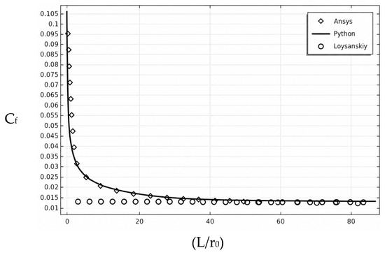
Figure 3. Comparison of friction coefficients on the pipe inner surface obtained from the model and ANSYS Fluent.

Figure 4 presents a comparative analysis of flow characteristics using both constant and variable thermophysical properties. The traditional constant-parameter model produced identical, overlapping results for $Pr=7,\hspace{0.17em}\hspace{0.17em}5\hspace{0.17em}\hspace{0.17em}\mathrm{and}\hspace{0.17em}\hspace{0.17em}2.5$, showing no variation in flow behavior. In contrast, accounting for the temperature-dependent properties $\mu \left(T\right), C_v\left(T\right)$ and $\lambda \left(T\right)$ revealed the significant influence of the temperature field on flow evolution.

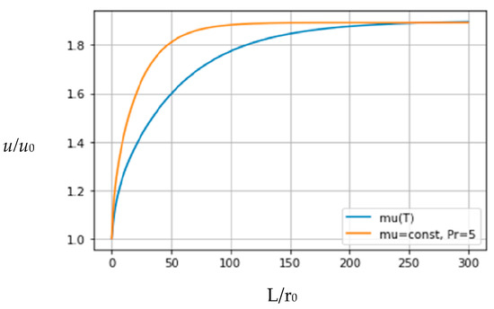
Figure 4. Re = 400, velocity profiles for the cases of constant μ and μ(T) (temperature-dependent viscosity).

The trends observed in the characteristic variation in pressure (Figure 5) are consistent with earlier findings. Constant property values produced the same results across different Prandtl numbers (Figure 5). However, pressure drop decreased when variable kinematic viscosity, specific heat and thermal conductivity were considered. Under these conditions, the velocity profiles adjusted more slowly, resulting in reduced pressure loss.

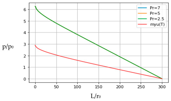
Figure 5. Re = 400, pressure distribution.

The model curve shows close agreement with the Comsol Multiphysics results in both the central and transitional areas. Overall, the findings demonstrate a high level of correspondence between the model and Comsol Multiphysics, supporting the model’s validity and its capability to describe radial heat transfer in a sensible and reliable manner (Figure 6).

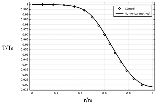
Figure 6. Radial temperature distribution Re = 400, z = L.

Figure 7 compares the temperature development at the center of the pipe obtained using the developed numerical algorithm written in Python with the simulation obtained using COMSOL Multiphysics. As can be seen, the COMSOL Multiphysics output is oscillatory in the early stages of heat propagation during the transient (non-stationary) regime. Conversely, the curves obtained using the proposed solution algorithm do not exhibit these oscillations, and the temperature evolution is smoother and more stable. Moreover, in regions where oscillations are absent, the COMSOL Multiphysics results are almost identical to those generated by the proposed model, with an absolute overlap in the curves. This confirms the validity and soundness of the numerical method developed to explain heat transfer at the center of the pipe. The mathematical model can therefore be used to determine temperature and flux of the flow, assess the efficiency of heat transfer, and assess fluid flow under laminar flow conditions.

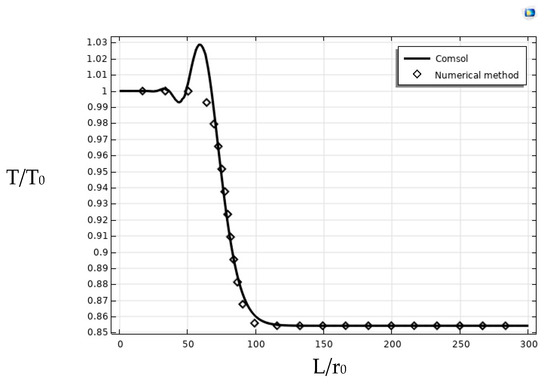
Figure 7. Comparison of the temperature variation along the pipe axis between the model and Comsol Multiphysics results, Re = 400.

4. Discussion

The results of this study demonstrate that the developed model reliably reproduces the key characteristics of laminar flow and heat transfer in cylindrical channels. Comparison with Comsol Multiphysics simulations shows strong agreement for both temperature and velocity profiles, confirming the model’s accuracy in capturing the essential flow dynamics.

Analysis of wall shear stress and friction coefficients shows that the model correctly captures the inverse relationship between hydraulic resistance and Reynolds number in the laminar regime. Variable fluid properties, such as kinematic viscosity and thermal conductivity, slightly delay the development of fully developed velocity profiles, thereby reducing the pressure drop and highlighting the influence of the thermal boundary layer on flow development. Furthermore, the axial velocity distribution near the inlet aligns well with the classical quadratic Poiseuille profile, confirming that the model accurately represents both entrance and fully developed flow conditions.

The effects of temperature on flow velocity and pressure were also examined, revealing that variations in fluid properties and thermal conditions can significantly affect flow behavior. Overall, these findings validate the proposed modeling approach, demonstrating its ability to predict flow dynamics, heat transfer, and energy losses under laminar conditions. The results provide a solid foundation for optimizing cylindrical channel designs and can be extended in future research to investigate more complex geometries, variable fluid properties, or transient flow conditions.

5. Conclusions

In typical heat transfer problems in fluids, the Prandtl number (Pr) is often assumed constant, which limits the representation of the process and neglects the effect of temperature-dependent viscosity (μ) on local Reynolds number (Re). In this study, the proposed solution algorithm accounts for temperature-dependent fluid properties, including μ(T), $c_p\left(T\right)$ and $\lambda \left(T\right)$ for an incompressible Newtonian fluid.

The results demonstrate that incorporating temperature-dependent properties yields a more accurate representation of flow and heat transfer than approaches assuming a constant Pr. The model accurately captures the effects of variable viscosity, specific heat, and thermal conductivity on velocity profiles, temperature distribution, wall shear stress, and pressure drop. This approach enables reliable prediction of laminar flow dynamics and energy transport under conditions where fluid properties vary with temperature.

Overall, the developed methodology offers a robust and efficient approach for analyzing laminar flow with heat transfer in cylindrical channels. It provides a solid foundation for optimizing channel designs and can be extended in future research to study more complex geometries, transient flow conditions, and fluids with temperature-dependent properties.

References

- Graetz, L. Ueber die Wärmeleitungsfähigkeit von Flüssigkeiten. Ann. Phys. Chem. 1885, 25, 337–357. [Google Scholar] [CrossRef]
- Nusselt, W. Die Abhängigkeit der Wärmeübergangszahl von der Rohrlänge. Z. Vereines Dtsch. Ingenieure 1910, 54, 1154–1158. [Google Scholar]
- Happel, J. Hydrodynamics at Low Reynolds Numbers; Mir: Moscow, Russia, 2016; 632p. [Google Scholar]
- Moshinsky, A.I. Dimensionality Theory in Problems of Chemical Engineering; Lambert Academic Publishing: Saarbrücken, Germany, 2017; 94p. [Google Scholar]
- Ananikov, S.V. Temperature field during fluid flow in a semi-infinite prismatic channel of triangular cross-section (boundary conditions of the first kind). Bull. Kazan Technol. Univ. 2012, 6, 147–150. [Google Scholar]
- Rubtsova, L.N.; Aleksandrova, L.Y.; Ganin, P.G.; Markova, A.V.; Moshinsky, A.I.; Sorokin, V.V. Study of laminar flow in prismatic channels of rectangular and elliptical cross-section. ChemChemTech 2022, 65, 93–100. [Google Scholar] [CrossRef]
- Valueva, E.P.; Purdin, M.S. Pulsating laminar flow in a rectangular channel. Thermophys. Aeromechanics 2015, 22, 622–625. [Google Scholar] [CrossRef]
- Yulmukhametova, R.R.; Musin, A.A.; Kovaleva, L.A. Numerical modeling of laminar suspension flow in a flat channel. Bull. Bashkir Univ. 2021, 26, 281. [Google Scholar] [CrossRef]
- Gavrilov, A.A.; Minakov, A.V.; Dekterev, A.A.; Rudyak, V.Y. Numerical algorithm for modeling laminar flows in an annular channel with eccentricity. Sib. J. Ind. Math. 2010, 13, 3–14. [Google Scholar] [CrossRef]
- Fafurin, A.V.; Fafurina, E.A. Kinematic structure of swirling flow. Bull. Kazan Technol. Univ. 2011, 14, 43–46. [Google Scholar]
- Abbasov, E.M.; Imamaliev, S.A. Mathematical modeling of two-phase fluid motion in concentrically located communicating pipes. Eng. Phys. J. 2014, 87. [Google Scholar]
- Chesnokov, Y.G. New formulas for calculating the characteristics of liquid or gas flow in a pipe of circular cross-section. Eng. Phys. J. 2017, 90, 1005–1011. [Google Scholar]
- Girgin, I.; Turker, M. Axial heat conduction in laminar duct flows. J. Nav. Sci. Eng. 2011, 7, 30–45. [Google Scholar]
- Naqiuddin, N.H.; Saw, L.H.; Yew, M.C.; Yusof, F.; Ng, T.C.; Yew, M.K. Overview of micro-channel design for high heat flux application. Renew. Sustain. Energy Rev. 2018, 82, 901–914. [Google Scholar] [CrossRef]
- Khujaev, I.; Hamdamov, M.; Ravshanov, S. Numerical study of fluid flow and heat transfer in a relief pipeline with variable diameter. Math. Models Eng. 2025, 11, 243–258. [Google Scholar] [CrossRef]
- Khujaev, I.; Shirinov, Z.; Ravshanov, S. Mathematical Model and Calculation Algorithm Modern Heat Exchanger Connected to a Two-Pipe Heating Network. AIP Conf. Proc. 2025, 3265, 060002. [Google Scholar] [CrossRef]
- Ravshanov, S.; Aminov, K.; Rahmonova, N. Simulation of Flow Dynamics in a Gas Network Pipe. AIP Conf. Proc. 2025, 3265, 060007. [Google Scholar] [CrossRef]
Disclaimer/Publisher’s Note: The statements, opinions and data contained in all publications are solely those of the individual author(s) and contributor(s) and not of MDPI and/or the editor(s). MDPI and/or the editor(s) disclaim responsibility for any injury to people or property resulting from any ideas, methods, instructions or products referred to in the content. |
© 2026 by the authors. Licensee MDPI, Basel, Switzerland. This article is an open access article distributed under the terms and conditions of the Creative Commons Attribution (CC BY) license.