


Abstract
In this paper, the formulation and method of implementation of boundary conditions for heterogeneous reactions in porous media are elaborated. These are implemented into a previously validated lattice Boltzmann model for the simulation of heterogeneous reactions in porous media, extending it on multiple fronts. The formulation of the boundary conditions is validated thoroughly. The conversion of solid carbon to CO and CO2 is chosen as a specific case of application. An extensive parametric study is conducted with a specific geometry consisting of spherical substrate particles, coated with a reactive soot layer, to highlight the capability of the code. The code was able to capture the expected evolution of a combustion front and the influence of process parameters onto its propagation velocity. The propagation speed linearly increased with an increase in the reactant mass fraction and exponentially increased with Péclet number. Also, the CO/CO2 ratio obtained from experimental data could be reproduced with good accuracy. Furthermore, an algorithm for the correct evaluation of the specific surface is presented, which is necessary for evolving solid domains based on realistic geometries containing enclosed cavities. The method of implementation, computational overhead and acceleration technique are discussed. Finally, the model and all boundary conditions are extended to 3D and validated.
1. Introduction
Heterogeneous reactions in porous media play a significant role in many different fields of application, ranging from packed bed reactors in chemical process engineering to the study of reactions in soil in agricultural sciences, novel hydrogen storage methods and more [1,2]. The simulation of these systems, taking into account the intricate interplay of different physical phenomena, including fluid dynamics, conjugate heat transfer, species conservation with reactive sources and sinks, as well as reactive heat release, while considering realistic, non-regular structures, is a non-trivial problem.
Due to its mesoscopic nature, the lattice Boltzmann method (LBM) is well suited to tackle these multi-physics simulation tasks. Further advantages are the straightforward implementation of complex geometries [3,4], since the domain is discretized by an equidistant mesh. The classic LBM discretizes the Boltzmann equation explicitly in time, resulting in fully local transport equations, which can be solved independently in a parallel manner on each lattice node. However, only a few publications exist in which the LBM is used for the simulation of heterogeneous reactions. Xu et al. [5] made use of a single relaxation time (SRT) model for simulating heterogeneous reactions in porous media, implementing a thermal counter-slip method for the description of conjugate heat transfer at the solid–gas interface. Yamamoto [6] developed an incompressible LBM model, which he used to conduct filter-scale simulations. Furthermore, Lei et al. [7] proposed a weakly compressible lattice Boltzmann model and conducted simulations of soot combustion in 2D porous media. Guo et al. [8] used the lattice Boltzmann method to model chemical adsorption processes for thermochemical energy storage applications while considering the hydration reaction inside of a non-regular solid domain. Wang and Zhu [9] employed a multi-relaxation-time LBM expression to describe the ablation of carbon fibers. Other approaches include the usage of diffuse interface models to track the evolution of the solid geometry, as shown in [10]. Furthermore, publications exist for other types of heterogeneous reactions, including the conversion of levulinic acid to -valerolactone [11], the investigation on dissolution and precipitation [12] or general descriptions of heterogeneous reactions [13,14]. An overview of the LB method for the description of reactive flows can be found in [15]. However, LBM studies of heterogeneous reactions are usually restricted to 2D simulations, or a coupled method is used, in which the LBM is applied for the calculation of the velocity field, and the finite volume method is used for the calculation of the thermal and component fields.
The method used in this paper is based on the LB model proposed by Lei et al. [7], with several differences. The first change is the method used for the description of the conjugate heat transfer at the interface between the solid and gas phases. While Lei et al. [7] use an explicit method proposed by Karani and Huber [16], which treats the conjugate heat transfer by introducing additional force terms in the collision step of the energy conservation equation, a different method, proposed by Li et al. [17] is used in the present paper. As was found in [18], the method of Li is able to accurately describe the conjugate heat transfer at the interface considering the heterogeneous reaction, while also offering several advantages regarding the computational efficiency and the ease of treatment of complex boundary geometries. The second difference between the model used in this paper and the base model of [7] is the implementation of the reaction heat. As was described in detail in [18], the reaction heat is split up, considering the densities and specific heat capacities of both phases, and then partially added to either phase, ensuring a continuous temperature profile across the interface.
With the base model for the 2D case being extensively validated in the previous publication of the authors, we propose additional boundary conditions and algorithms for use in studying realistic structures in this manuscript. To this extent, the three-dimensional formulation of the boundary conditions, as well as symmetry boundary conditions, are explained. Furthermore, the study of realistic soot structures, which might exhibit enclosed cavities, requires a method to precisely calculate the accessible reactive surface. To tackle this problem, the implementation of the breadth-first search algorithm is explained, which enables the analysis of the change of the reactive surface over the combustion progress while omitting enclosed cavities from the calculation of the reactive surface. The algorithm is applied to a simple academic test case and to a realistic soot sample, generated at the Institute of Chemical Process Engineering (ICVT) in Stuttgart.
Furthermore, a parametric study is conducted to investigate the influence of the Péclet and Damköhler numbers onto the reaction regime and to highlight the applicability of the code. Moreover, the inlet mass fraction of oxygen and the ratio of reactive and inert solid mass is varied. Subsequently, the evolution of the soot morphology during combustion is investigated using FIB-SEM images of real soot samples to define the solid geometry. It is noted that parts of the underlying data of this publication have previously been published in the PhD thesis of the main author [19]. The current manuscript differs in its focus, presentation, and interpretation, with an emphasis on methodological clarity and applicability.
2. Governing Equations
In this section, the governing equations used to describe the physical phenomena of a fluid flow consisting of multiple components, the thermal field, solid–fluid interaction, as well as heterogeneous reactions, are presented briefly. The same base model as described in [18] is used, with differences and extensions being highlighted specifically.
For the simulation of a fluid flow, the following two partial differential equations, representing the mass and momentum conservation, are needed.
In these equations, represents the density of the gas phase, denotes the vector describing the velocity field and t denotes the time. The nabla-operator ∇ represents the gradient operator, the pressure and external forces acting on the flow field, denoted, respectively, as p and , are included. Furthermore, the viscosity of the gas phase is denoted as . Since a heterogeneous reaction at the interface between the gas phase and the solid soot phase is to be described, n additional equations representing the mass conservation for the n components of the gas phase are needed. The mass conservation equations are shown in Equation (3) for the component. With the heterogeneous reaction being exothermic, the domain cannot be assumed to be isothermal anymore, and one additional equation is needed to describe the energy conservation. This is shown in Equation (4).
For clarification, it is mentioned that Equations (1)–(3) are used only in the gas phase of the domain, with Equation (4) being applied to both the solid and gas phases. Furthermore, the mass-fraction and the mass diffusion coefficient of the component are described as and , with specifying the consumption/production of component n at the solid–gas interface. The solid mass is tracked separately per voxel, with the full algorithm being described in Section 4.1. In the energy conservation equation, and T denote the specific heat capacity and thermodynamic temperature, with Q and denoting the source-/sink-term, as well as the thermal diffusivity, respectively. The heterogeneous reaction at the interface of solid soot and gas is assumed to be of the first order, and two different mechanisms are implemented, with the first one having carbon dioxide as the sole product. For this, the chemical equation is shown as [20]:
For a reaction of the first order, the reaction rate, when described by the Arrhenius formalism, is only proportional to the local concentration of one component. This assumption holds here since oxygen is the only gaseous reactant, with carbon being solid. Consequently, the reaction rate, , is given by Equation (6) [7]:
In this equation, A and denote the two kinetic parameters of the Arrhenius formalism, namely the pre-exponential factor and the activation energy of the reaction, respectively, with denoting the molecular weight of oxygen and R being the ideal gas constant. The reaction heat can then be calculated as the product of the reaction rate and the standard enthalpy of reaction , as:
The second mechanism additionally contains the carbon-monoxide forming reaction, which is shown in Equation (8):
Consequently, the reaction kinetics of the CO-formation are given by Equation (9), employing different kinetics parameters and :
The total reaction heat can then be calculated as the sum over all reactions, i, of the product of the reaction rate and the standard enthalpy of the reaction :
Also, the boundary conditions at the solid–gas interface need to be specified. For the flow field, the no-slip boundary condition is assumed, which can be described by Equation (11). For the component fields, the mass flux of the component normal to the interface has to coincide with the consumption/production by the chemical reaction. This is depicted in Equation (12), with the surface-normal mass and the consumption/production of the chemical reaction being shown on its left- and right-hand sides, respectively.
Here, is the stoichiometric coefficient of the component in the respective chemical equation. To complete the set of boundary conditions, the continuity of the temperature profile across the interface and the equity of the energy flux on either side of the interface have to be ensured. These characteristics are described, respectively, by:
and
in which the thermal diffusivity is denoted as , and the subscripts + and − describe the two sides of the interface. It is noted that the energy conservation at the interface comprises not only the diffusive and advective flux on either side of the interface but also the heat release caused by the chemical reaction. Furthermore, it has to be noted that the advective flux on the solid side of the interface vanishes. Due to the specific LB method used in this paper, with interfaces being assumed halfway between lattice nodes, the interface is always between lattice nodes assigned to both phases and never right on a lattice node. For this reason, the heat release of the reaction is split and added onto either side of the interface. In order not to violate the condition of the continuity of the temperature profile across the interface, i.e., Equation (13), the heat release has to be split up, considering the densities and specific heat capacities of the two media on either side of the interface. Consequently, the ratio of the specific heat capacities and densities of the solid (subscript s) and gaseous (subscript g) phases is defined as:
Subsequently, the fraction of the heat added to the solid and gaseous phase, and , respectively, can be calculated as:
A detailed description of the necessity of this splitting rule can be found in our previous study [18], in which the incorporation of the reaction heat onto either side of the interface was studied. Since the halfway bounce back LBM approach is used, the interface is located in between two interface nodes, one on the gas side and another one on the solid side. It was found that, to satisfy continuity of the temperature profile across the interface, the presented splitting rule is necessary. To facilitate a comparison of test cases and simulation parameters, the following dimensionless numbers are introduced:
These include the Péclet number , which is the ratio of the advective flux u and the diffusive reactant transport , and the Damköhler number ), which relates the reaction kinetics k to the diffusive reactant transport. Here, is the characteristic length scale of the problem.
3. Lattice Boltzmann Method
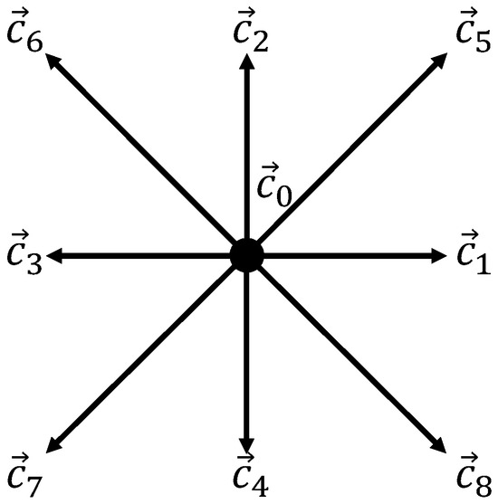
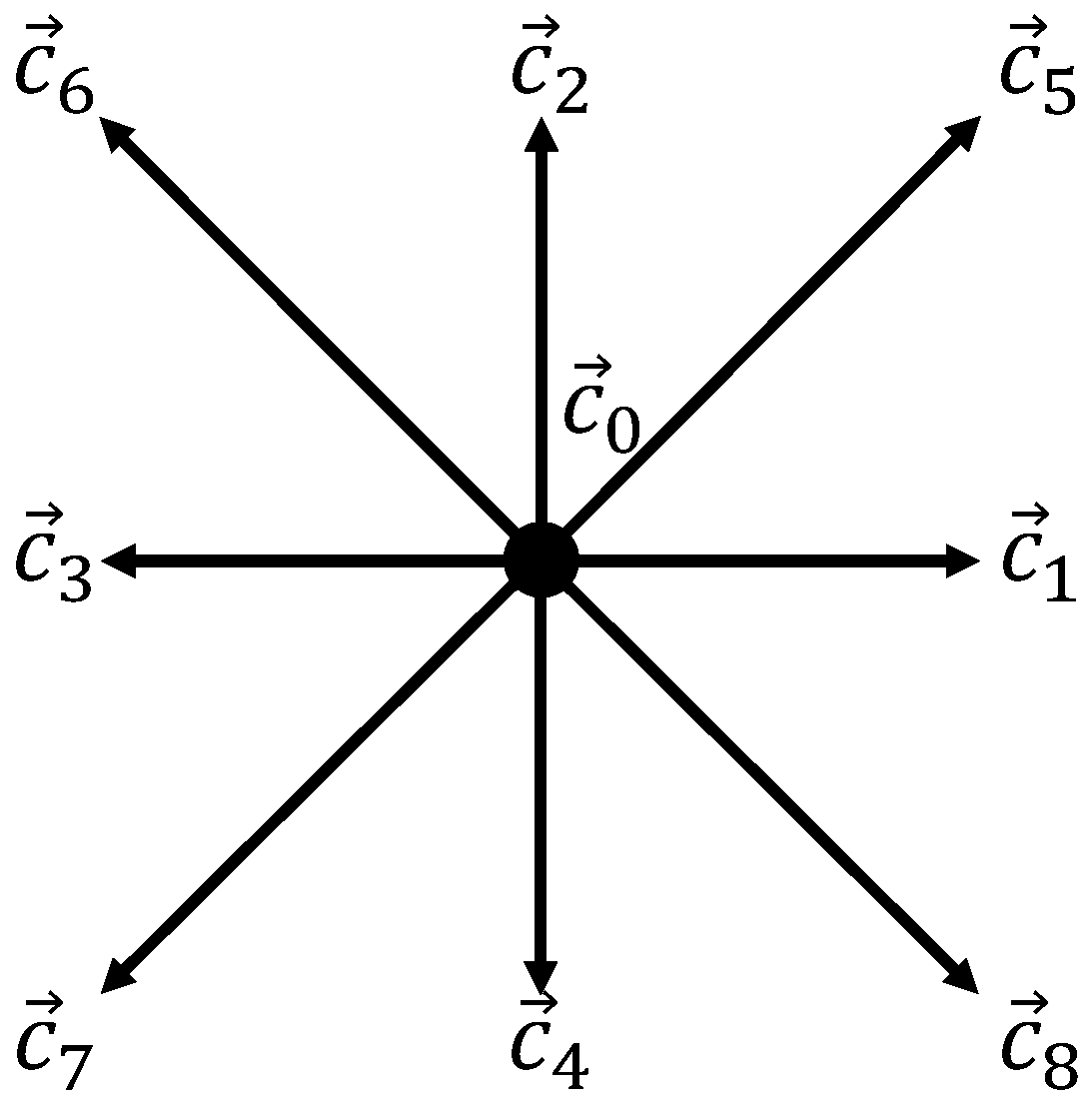
In this section, the lattice Boltzmann expression of the equations presented above is introduced. For the two-dimensional case, the D2Q9 lattice is used, following the nomenclature presented in [21]. As shown in Figure 1, it exhibits one lattice velocity residing on the node, as well as four diagonal and two horizontal and vertical lattice velocities, respectively.
Figure 1.
D2Q9 lattice velocity scheme.
For this discretization scheme, the vectors specifying the lattice velocities are given as:
The lattice speed c is defined as the ratio of the spatial and temporal discretization size. Also, the values of the lattice velocity and of the weighting factors are inherent to the lattice used and are defined as:
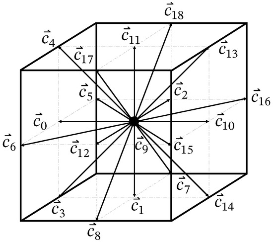
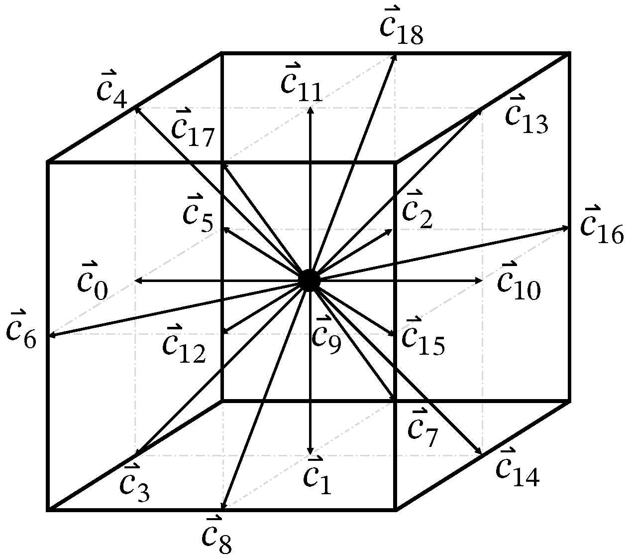
For the three-dimensional cases, a D3Q19 lattice is used, which exhibits one lattice velocity residing on the node, as well as six face-connecting and twelve edge-connecting velocity vectors, as shown in Figure 2.
Figure 2.
D3Q19 lattice velocity scheme.
The weighting factors for the residing (0), the face-connecting (1) and the edge-connecting (2) lattice velocities are presented in Equation (20):
With the lattice-discretization chosen, the expression of the conservation equations can be determined. The LB equation for the flow field, the transport equation of the components and the energy conservation are given as following [7]:
Here, , and represent the distribution functions for the flow field, for the component and for the temperature, respectively. It is stated that this model accounts for density variations in the weakly compressible limit of standard LBM formulations, meaning that the thermal expansion introduced by heat released by the heterogeneous reaction cannot be accounted for fully. Here, all distribution functions in Equations (21)–(23) are vectors, indicated by the little arrow, since a multi-relaxation time (MRT) method is used. This means that the vectors, exemplary for the flow field , contain the distribution functions for all lattice velocities . For simulations with high Péclet numbers (Pe » 1), meaning negligible physical diffusivity, the MRT method offers several advantages regarding numerical artifacts, such as lattice anisotropy and numerical diffusion. When employing the MRT method, a collision happens in moment space, rather than lattice space. This means that, depending on the choice of the relaxation matrix, S, different moments can be relaxed at different rates, such that the influence of truncation errors can be mitigated. It is noted that, depending on the choice of the relaxation matrices, the MRT method reverts back to the SRT method. In this work, both the MRT and SRT methods are used, and no difference for the given range of values of the parameters, as defined in Section 5, was noted.
The spatial coordinates and the time-step size are denoted as and , respectively. Furthermore, the transformation matrix M is specified to transform the distribution functions from lattice space to moment space, in which the collision operation, the first summand on the right-hand side of each equation, is performed by the respective relaxation matrix, S, and , in MRT models. In Appendix C, the full definition of the relaxation matrices is given. The collision operator relaxes each distribution function towards its respective equilibrium distribution function, which are defined as:
The last summands in each equation introduce forcing-terms of varied heritage, i.e., external forces acting onto the flow field, or source terms in the temperature field.
Consequently, the macroscopic variables for each conservation equation can be determined by the moments of the respective distribution functions. As such, the density and the velocity field can be calculated as the 0th- and 1st-order moments of the distribution function f, the mass fraction of the component is calculated as the 0th order moment of and the thermodynamic temperature is given by the 0th order moment of h, as shown in the following:
Also, the pressure is coupled to the density by the following expression:
The entries of the external force vectors, denoted by the subscript i, are implemented according to the method proposed in [22], which results in:
In these equations, refers to an arbitrary force vector acting onto the flow field, with the force vectors for the component and temperature fields given as:
4. Numerical Methods
4.1. Mass Consumption
As validated in our previous work [18], the code is capable of the simulation of a gas flow, consisting of multiple components, and of the temperature field, in a porous medium. Furthermore, the code contains an algorithm for the simulation of conjugate heat transfer and heterogeneous reactions at the solid–gas interface. Hereby, the solid medium is assumed to have infinite mass, leading to a constant solid geometry and flow field with transient temperature and component fields. Subsequently, the code is extended to deal with the transient consumption of the solid soot structure, resulting in the temporal evolution of the soot morphology with progressing combustion. This is achieved by allocating a specific amount of mass to each lattice node of the solid domain. The respective amount of mass is calculated based on the parameters and reference values of the LBM simulation. Based on the conversion factors and resulting values for the distance between lattice nodes and density , both in lattice units, the mass assigned to one solid lattice node, , can be calculated as:
In the three-dimensional case, the volume of a lattice node is described by . For two-dimensional cases, the domain is assumed to be of thickness 1 in the third direction, resulting in the same formula for the calculation of the mass of a lattice node. For the parameters given for the combustion test case presented in [5], the calculation of the mass per lattice volume in SI units, , and in lattice units, , is performed as:
With the exact amount of mass assigned to each lattice cell, the combustion progress of one lattice node can be tracked by integrating the reaction rate at each interface pane over time and comparing it with the total initial mass of the respective node. By using the reaction rate at the solid–gas interface in [mol m−2 s−1], which was defined above in Equations (6) and (12), describing the mass conservation of the component at the interface, the mass fraction of oxygen at the interface can be calculated by following Lei et al. [7]:
Here, the mass fraction of oxygen at the lattice node in the gas phase adjacent to the interface is described as . It is noted that Equation (40) can be evaluated both in lattice units and SI-units, assuming consistent unit transformation. Also, a detailed description of the transformation of SI units to lattice units can be found in [18], with a brief summary being shown in Appendix E. With this value acquired, the reaction rate can be calculated by Equation (6) [mol m−2 s−1] and translated into a mass-specific consumption rate of carbon by multiplying it with the stoichiometric coefficient and the molar weight of carbon, , for the respective reaction, as shown in the following:
Multiplying the mass-specific consumption rate with the surface area of the lattice faces results in the total mass consumption rate at the respective lattice node. This value is integrated over time to calculate the total amount of mass, which was already consumed for each solid lattice node. In each time step, after performing the collision and streaming steps, the total mass consumed at each solid lattice node is compared with the initial mass of the lattice node, and the combustion progress is calculated in %. If the progress reaches 100%, which indicates the total consumption of the soot content of the respective lattice node, the flag of this node is switched to “bulk”, and the distribution functions for the density and components need to be initialized.
Said initialization is crucial since an inconsistent initialization can lead to oscillations not only in the density and component fields but also in the velocity field. This, in turn, affects every other conserved quantity, like the temperature field, as well. The initialization of the distribution functions after a cell switch can be conducted by taking the average of the macroscopic variables, i.e., density and mass fractions of the components, from all neighboring cells, which are attributed to the flow domain.
This method leaves room for improvement since oscillations in the flow field can be observed. These non-consistent values in the velocity field propagate through their dependency into all other transported scalars, for example, the temperature field and the component fields. For this reason, the distribution functions are initialized as described above, and their values are relaxed towards the values, which are consistent with the surrounding lattice nodes, by performing the collision and streaming step locally for the switched node before continuing in the propagation of time with the whole domain. In these streaming steps, the distribution functions are not streamed out to neighboring cells (leading to oscillations), but only neighboring distribution functions are streamed to the initialized cell. With this method, the values of the distribution function at the switched cell can relax towards a consistent equilibrium value without affecting the cells around it, thus inhibiting oscillations and enabling an initialization with consistent values.
4.2. Symmetric Boundary Condition
For the simulation of repetitive domains, which exhibit a symmetry line, it is possible to save computational resources by defining a symmetry boundary condition for the LB method, enabling the simulation of the full test case by performing the LB algorithm on just half of the domain. Figure 3 shows an example of the combustion test case, which was presented by [5] and which was used in our previous work to validate our LB model [18]. Contrary to the depiction in the mentioned literature, a symmetry line is added in blue and the top half of the domain is removed. If a symmetric boundary condition is imposed in a proper manner, the computational cost of the domain can be split in half.
Figure 3.
Combustion test case as presented in [5], with symmetry line. B denotes the width of the channel, b denotes the width and spacing of the solid obstacles.
In order for the boundary condition to be symmetric, it has to satisfy multiple conditions. The boundary condition has to impose a zero gradient of all scalar variables, as well as of the components of the velocity field perpendicular to the symmetric boundary. Furthermore, the transport of scalar variables, as well as a boundary velocity parallel to the symmetric boundary, has to be possible. These conditions are satisfied by the so-called specular reflection boundary condition [23], which is typically used to impose free-slip boundaries. Here, the normal component of the fluid velocity is assumed to be zero at the wall, with the tangential component not being influenced. Essentially, the boundary is assumed to be non-penetrable with no shear-stress being imposed.
This results in the distribution functions, whose lattice velocity vectors are perpendicular to the boundary, to be reflected, similar to the classical bounce-back algorithm. The distribution functions, which intersect the boundary condition at an angle, are mirrored at the boundary condition. This process can be performed in both a local and non-local manner, as subsequently shown:
For an extensive comparison of both methods regarding convergence and accuracy, the reader is referred to [24].
4.3. Extension of Boundary Conditions to 3D
When performing LBM simulations in 3D, rather than 2D, some boundary conditions have to be redefined. The external boundary conditions, namely the zero-gradient boundary condition for the scalar variables of temperature and mass fraction of the component, can be determined in analogy to the 2D algorithm for the anti-bounce-back method, as proposed in [25]. However, the Zou-He boundary condition, which is used to impose a zero gradient for the velocity field at the outlet of the domain, has to be adapted for the case of a three dimensional simulation. By performing the derivation procedure, as described in [26], and adapting it to the D3Q19 discretization scheme, the following expression for the missing distribution functions can be derived:
These values correspond to the left plane of the lattice velocities, as shown in Figure 2.
4.4. Calculation of Effective Reactive Surfaces
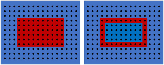
As described earlier, the main parameter for the comparison between experimental and computational soot combustion will be the temporal evolution of the reactive surface of the soot geometry as a result of combustion. Therefore, an algorithm for the calculation of the reactive surface at each time step is needed. A trivial idea would be to iterate over all lattice nodes associated with the solid domain, to compare its property with the properties of all neighboring nodes, and to sum up all interfaces by means of multiples of the lattice distance . This, however, does not result in the correct value of the reactive surface, as is demonstrated by Figure 4.
Figure 4.
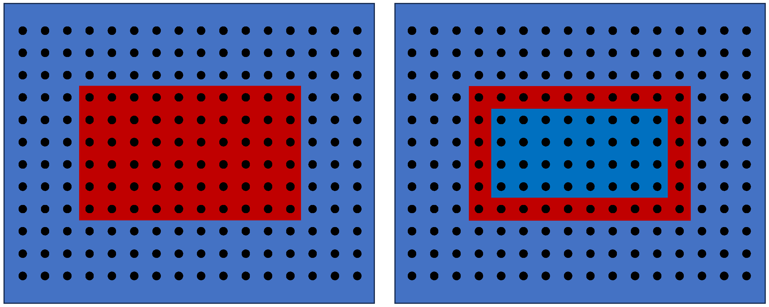
Solid obstacle without (left) and with (right) cavity, resulting in different values for the reactive surface, as calculated by the rudimentary algorithm. The solid domain is depicted in red, with the void space being depicted in blue.
When iterating over all solid nodes (depicted in red) and summing up the interfaces, the rudimentary way to calculate the accessible reactive surface will result in the value of 32 for the case of a solid obstacle without cavities (left case). For the case of a solid obstacle with cavities, which are not connected to the surrounding gas phase (right case), the algorithm would wrongfully conclude that the inner surface is “accessible reactive surface”, resulting in a value of 56. It becomes apparent that cavities with no connection to the surrounding gas phase have to be excluded from the calculation of the effective, accessible reactive surface. This can be achieved by using the “Breadth first search” (BFS) algorithm, originally invented by Konrad Zuse in 1945 and published shortly after [27]. With this algorithm, the lattice can be systematically propagated through from a given starting point, and the information of all nodes that are accessed throughout the propagation is stored in a tree-like data structure. A realistic 3D structure of soot, which was obtained by an FIB-SEM analysis of a real soot sample, exhibited a percentage of the cavity surface of 0.21%. However, different structures, especially closed-cell structures, involve a drastically higher percentage of closed cavities, making the usage of such an algorithm imperative. The implementation of the algorithm is explained in detail in Appendix B, and the 3D structure, with which it was tested, is shown in Appendix A. Moreover, the performance of the BFS algorithm can easily be increased by utilizing partial parallelization. The first and third main blocks of the algorithm shown in the Appendix contain only operations that can be executed in an independent manner, thus facilitating parallelization. The performance gain was then benchmarked for the realistic soot sample, shown in Appendix A, with a lattice resolution of 499 × 415 × 339 lattices, resulting in a total lattice count of 70.2 million cells. When comparing the performance of the parallelized BFS to the standard BFS, a performance increase of a factor of six could be reported, with a reduction in the execution time from 3 s to about 0.5 s on a 32 Core Ryzen Epyc 7313P. The BFS algorithm returned specific surface values in good agreement with the experimentally reported BET surface areas for soot samples of a comparable type and morphology, supporting the correctness of the 3D implementation in practical applications.
5. Results and Discussion
In this section, the proposed boundary conditions and the 3D extension are validated. Moreover, a two-dimensional test case is created to assess different combustion regimes, depending on the Péclet number, the Damköhler number and the inlet mass fraction of oxygen, , to highlight the capability of the model. It is noted that, similar to other discretization techniques for partial differential equations, when performing simulations with LBM, the convergence of the lattice resolution has to be confirmed. In this paper, a lattice discretization similar to what can be found in [5,7] is used. Furthermore, a mesh sensitivity analysis can be found in Appendix D.
5.1. Verification of Boundary Conditions and 3D Formulation
5.1.1. Symmetry Boundary Condition
Subsequently, the symmetry boundary condition is validated. For this, the combustion test case of [5], which has been used previously for the validation of the 2D model in [18], is applied again.
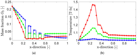
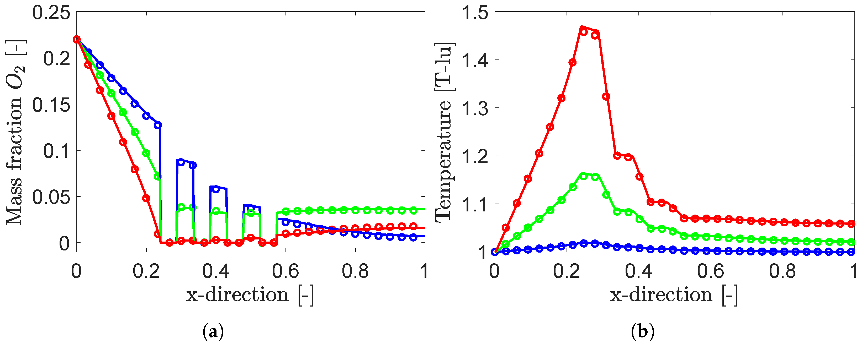
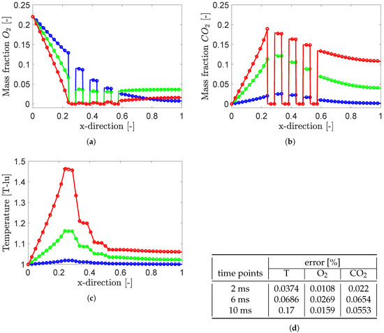
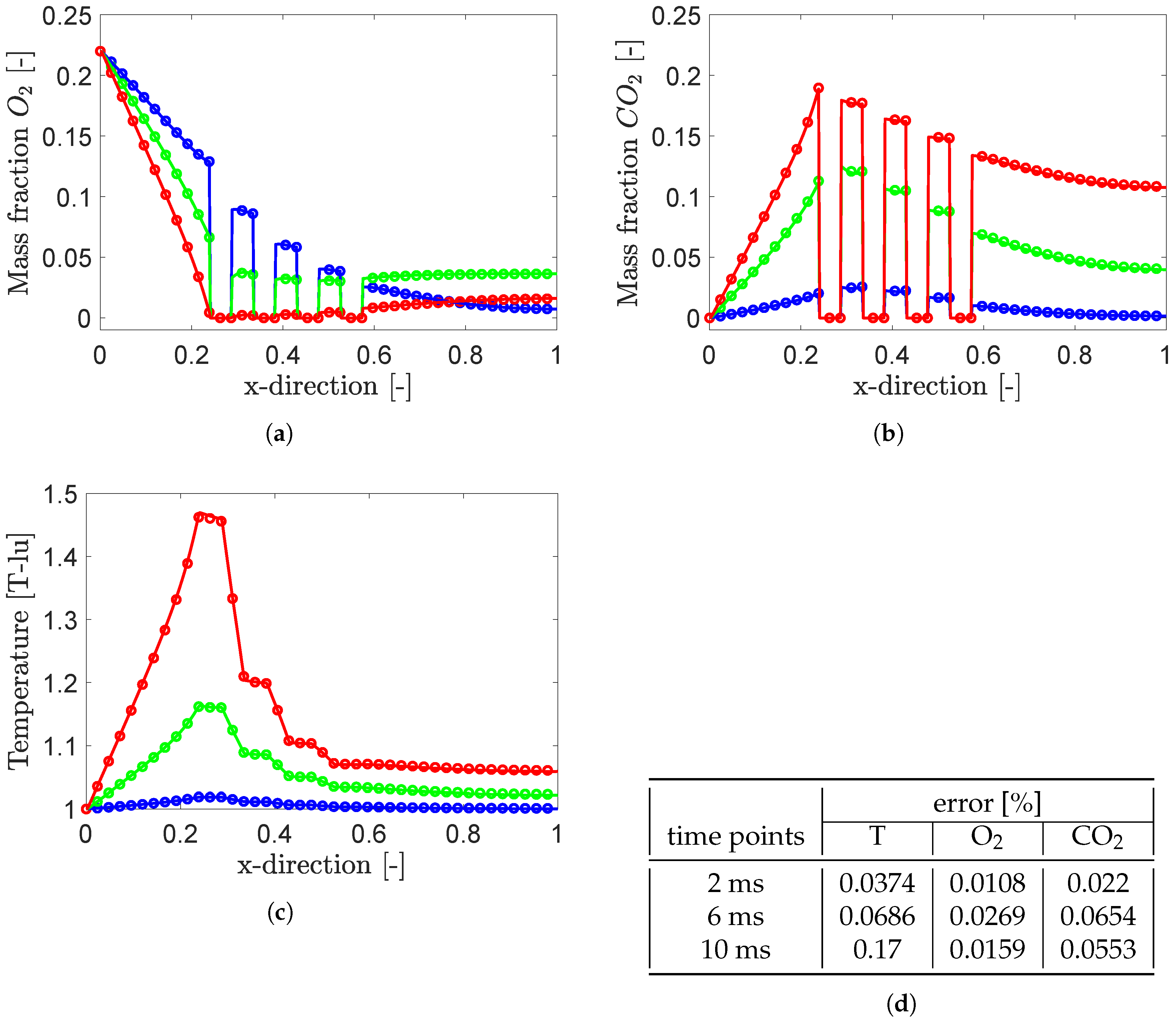
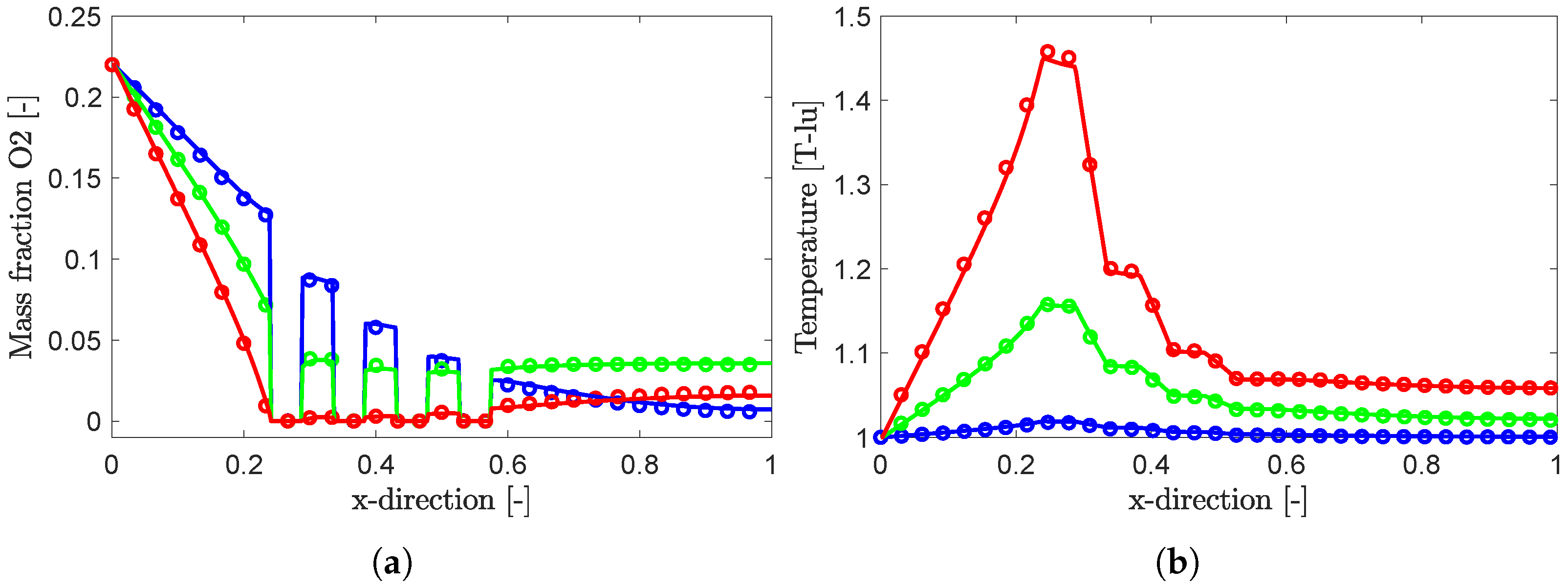
As shown in Figure 3, the domain of the combustion test case is symmetric, enabling the calculation to be restricted to half of the domain. This results in a resolution of 420 × 41 lattice nodes, with all parameters being chosen according to [5]. The resulting profiles of the mass fraction of O2 and the temperature at the symmetry line are shown in Figure 5. It can be seen that the results agree very well with the literature data for all three displayed times. For a quantitative analysis, the RMS error between the literature data and the simulations results is evaluated. For the temperature field, errors of , and are received at 2 ms, 6 ms and 10 ms. For the O2 and CO2 profiles at the given time points, errors of , and and , and are received.The direct comparison of the simulation with the full domain and with the reduced domain is shown in Figure 6.
Figure 5.
Validation of the symmetry boundary condition by comparison of the results with literature data [5]. In the graphic, (○) and (–) represent the literature data and the LBM results at 2 ms, (○) and (–) at 6 ms and (○) and (–) at 10 ms for the mass fractions of oxygen (a) and temperature (b).
Figure 6.
Comparison of the LBM results with and without symmetry boundary condition. Shown are the mass fraction of O2 (a), the mass fraction of CO2 (b), the temperature profile (c), and the RMS error values (d). In the graphic, (○), (○) and (○) represent the LBM simulation with the full domain at 2 ms, 6 ms and 10 ms, while (–), (–) and (–) represent the results of the simulation with the symmetry boundary condition.
The profiles along the symmetry line of the mass fraction of O2 and CO2, as well as the temperature and the RMS errors between, are shown. It becomes apparent that the implementation of the symmetry boundary condition marginally affects the results, with the largest RMS error being 0.17% for the temperature field after 10 ms. For the profiles of O2 and CO2, RMS errors smaller than 0.027% and 0.0654% are reported.
5.1.2. 3D Flow—Mass Conservation
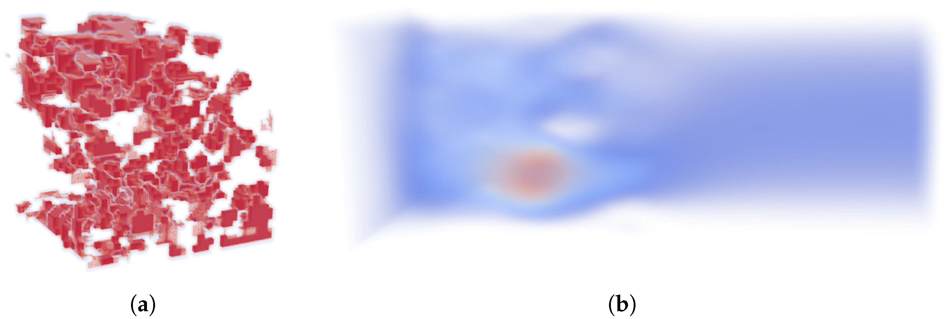
For the validation of the flow field, a squared tube with no-slip walls at the top and bottom, as well as in the back and front, is set up. The cross section has a lattice resolution of lattice nodes, and the domain has a length of 100 lattice nodes. At the inlet, a plug flow profile is imposed, and the outflow is defined by a zero-gradient Neumann boundary condition. Furthermore, the domain is filled with a three-dimensional porous structure, which is received by extracting a part of the full-size FIB-SEM geometry. The cubic porous medium has an edge length of 40 lattice nodes and is located 10 lattice nodes downstream from the inlet. The stationary solution of the velocity magnitude is shown in Figure 7, exhibiting the uniform velocity of the imposed plug flow at the inlet, subsequently describing a strongly disturbed velocity field inside the porous structure and forming the parabolic velocity profile of a fully developed flow in the outlet region of the domain.
Figure 7.
Solid soot domain (a) and stationary solution of the velocity magnitude (b) for the mass conservation test case.
At the inlet and outlet, the mass flow is calculated by multiplying the density with the velocity component perpendicular to the interface and integrating the mass flow over the inlet and outlet surfaces. As the stationary solution is reached, the deviation between inlet and outlet mass fluxes reaches 0.03262%.
5.1.3. 3D Heat Conduction
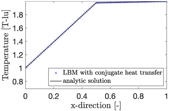
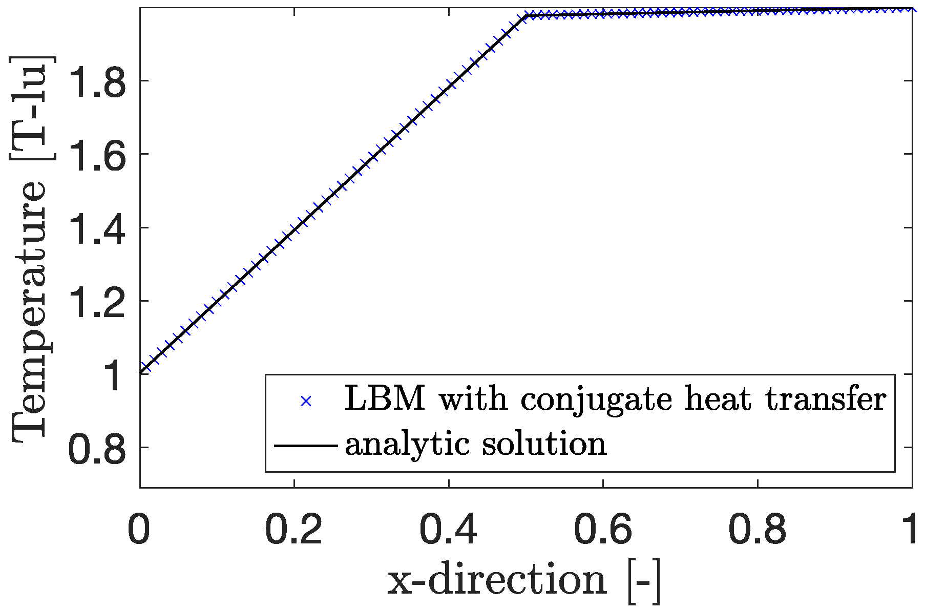
The heat conduction test case is set up in a similar manner to the one used for the two-dimensional validation. This results in a rectangular cross section with a lattice resolution of and three lattice nodes in the third dimension. On the short faces of the cross section, Dirichlet temperature boundary conditions are set. The long faces of the cross section are assumed to be adiabatic, and the third dimension is assumed to be periodic. For the imposed temperatures on the left and right side, the values of 1 and 2 in temperature lattice units are chosen. The stationary solution of the simulation, as well as the analytic solution for the given heat conduction test case, are shown in Figure 8.
Figure 8.
Analytic solution and results of the LBM simulation for the 3D heat conduction test case.
As it can be seen, the LBM simulation perfectly resembles the analytic solution, with an RMS error of .
5.1.4. 3D Temperature Relaxation
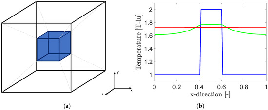
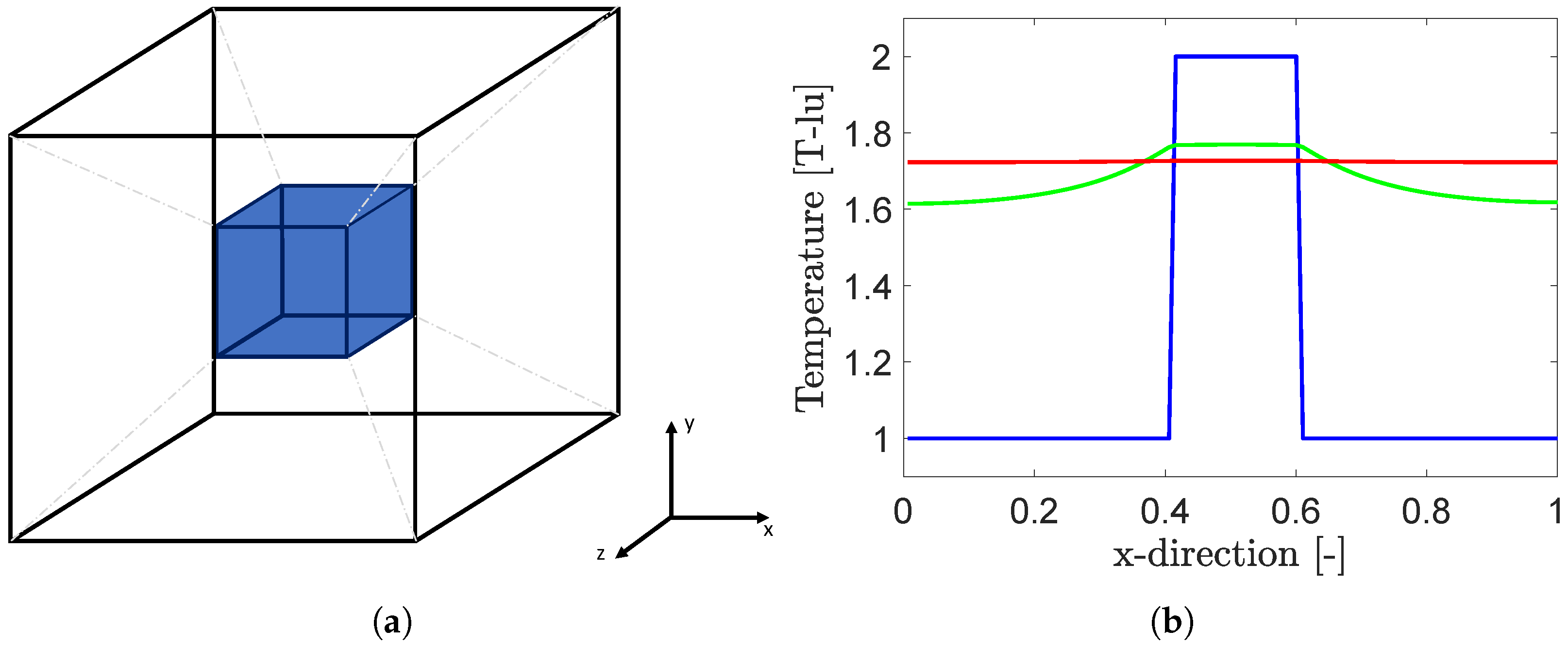
The test case used for the validation of the energy conservation in 3D is shown on the left in Figure 9. It consists of a cubic domain with a resolution of lattice nodes. A second cube with edge length of 20 lattice nodes, here displayed in blue, is located in its center. With the outer boundaries of the domain being assumed to be adiabatic, the energy within the system should be conserved. This is investigated by imposing a temperature profile onto the domain in such a way that the inner cube has an initial temperature of [T-lu], with the surrounding phase having an initial temperature of [T-lu]. This temperature profile will relax to a certain equilibrium value, which can be calculated based on the densities and specific heat capacities of the two domains, as well as the number of lattice nodes allocated to each domain. The simulation setup, as well as the temperature profiles along the centre line in the x direction, are shown in Figure 9.
Figure 9.
The domain for the 3D temperature relaxation test case consisting of a cubic domain, with a second cube centered in the middle of the domain. The inner cube is allocated the properties of coke, while the outer cube is assumed to be air. All six outer boundaries are set to be adiabatic (a), with resulting temperature profiles along the center line in the x direction (b). The initial condition is shown in blue, with the solution after 0.2 ms and 0.8 ms being shown in green and red.
The total thermal energy of the system increases slightly throughout the relaxation process, exhibiting an error of approximately . The analytical solution of the equilibrium temperature is calculated to be [T-lu], with the LBM simulation relaxing towards an equilibrium value of [T-lu].
5.1.5. 3D Combustion
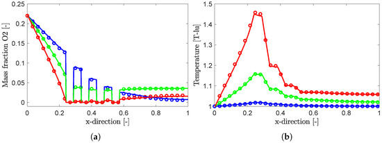
The 3D model is verified in analogy to the 2D verification, which was shown in [18], using the 2D test case presented first in [5], which is set up in 3D. For this purpose, a domain size of is chosen, and the geometry and boundary conditions are the same as in the 2D case, with the difference that the z-direction is assumed to be periodic. With this setup, the literature data of the 2D case can be used to verify the correct implementation of the 3D model. The D3Q19 velocity set includes diagonal velocity components in the third dimension. Consequently, this extension provides a meaningful consistency check, as the correct reproduction of the 2D solution in a 3D setting is only achieved if all velocity directions—including the diagonal components—are properly implemented. The resulting temperature and O2 profiles are shown in Figure 10. As can be seen, both temperature and O2 profiles exhibit excellent accordance with the literature data. Here, the RMS errors are , and for the temperature field, , and for the mass fraction of O2 and , and for CO2 at 2 ms, 6 ms and 10 ms.
Figure 10.
Validation of the 3D model by comparison of the results and the literature data [5]. In the graphic, (○) and (–) represent the literature data and the LBM results at 2 ms, while (○) and (–) represent those at 6 ms, and (○) and (–) represent those at 10 ms for the mass fractions of oxygen (a) and temperature (b).
5.2. Application Case: In Situ Crude Oil Combustion
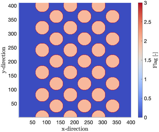
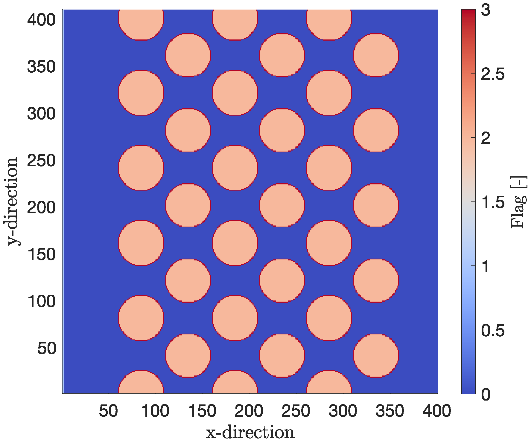
In this section, a test case to analyze dynamic combustion regimes on the μm scale, based on the in situ combustion in crude oil extraction, is presented. A square domain with the length of 400 μm in both the x and y directions is set up, as shown in Figure 11. Inside, round particles are arranged in a regular manner. The particles with a radius of 25 μm consist of an inert substrate carrier, depicted in orange (corresponding to a flag value of 2), which is coated with a reactive layer of soot of the thickness of 1 μm, depicted in red (corresponding to a flag value of 3). The pore space is filled with gas, here depicted in blue (eq. flag value 0). The distance between the centers of the particles in the x and y direction are 100 μm and 78 μm, respectively, with the smallest distance between particle centers being 63.4 μm in a diagonal direction. This results in an initial porosity of 65.36% before the consumption of the solid by combustion.
Figure 11.
2D test case consisting of circular inert substrate particles, which are ordered in a regular manner and covered by a reactive soot layer (red).
At the top and bottom of the computational domain, periodic boundary conditions are assumed, with the inlet being on the left side and the outlet being on the right sides. At the inlet, a velocity profile, as well as a static value for the temperature and the mass fractions of all components, are defined. At the outlet, a zero gradient boundary condition is assumed. The domain is assumed to be filled with pure nitrogen gas at the temperature , and the stationary solution for the velocity field corresponding to the mentioned boundary condition is used as the initial condition. The total set of parameters used for the simulations is displayed in Table 1.
Table 1.
Parameter set for the in situ crude oil combustion following [5].
It is noted that the physical properties of the gas phase are assumed to be constant for the simulations. Combustion simulations are performed for varying inlet temperatures between 500 °C and 900 °C, for inlet mass fractions of oxygen between and and for different inlet velocities, corresponding to Péclet numbers of 0.001 and 1, respectively.
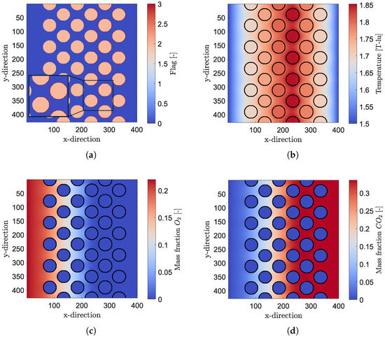
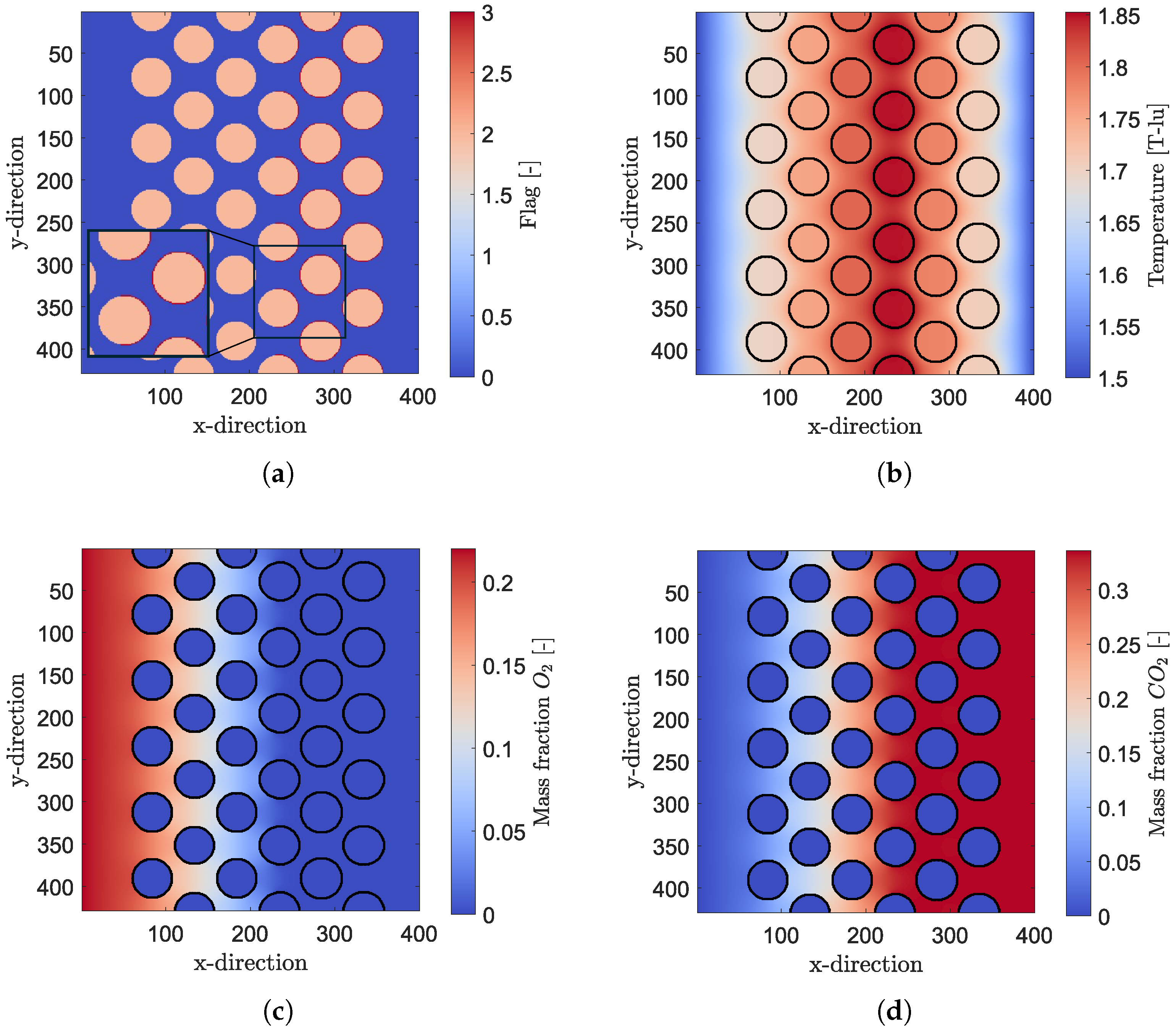
The result of one exemplary simulation is shown in Figure 12, in which the composition of the domain, displayed by the flag, denoting the different phases (a) and the temperature field (b) are shown. Furthermore, the mass fraction of oxygen and carbon dioxide is shown in Figure 12c,d at , respectively. The exemplary simulation was conducted with an inlet temperature of 1.5 temperature lattice-units (T-lu), corresponding to a temperature of around °C, with and an inlet mass fraction of oxygen of . It can be seen in Figure 12a that the reactive carbon layer has been burnt off completely on the first three columns of particles. Combined with the fact that the mass fraction of oxygen in Figure 12c fully depletes in the middle of the particles of the fourth column, and a temperature spike at the same position, it can be concluded that the combustion is limited by the mass transport of the reactant. This leads to a combustion front propagating through the domain from inlet to outlet, meaning that the reactive carbon layer on the particles is not consumed uniformly throughout the domain.
Figure 12.
Exemplary test case for 2D combustion with the simulation domain (a), a temperature field (b), the mass fraction of oxygen (c) and the mass fraction of carbon dioxide (d) at t = 1.2 s. A combustion front is visible, which is distinguished by the temperature increase and the consumption of the soot layer at pixel index 230 in the x-direction. For visualization purposes, the solid–gas interface is outlined in black.
In the following, the combustion behavior is analyzed using a variation of the Péclet number, the Damköhler number and the mass fraction of reactant at the inlet. The temporal evolution of the front position, the burning rate and the residual coke mass are used as characteristic parameters for the evaluation of the results. Furthermore, the maximum temperature of the combustion front over time will be analyzed.
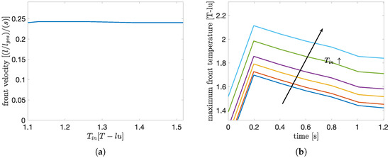
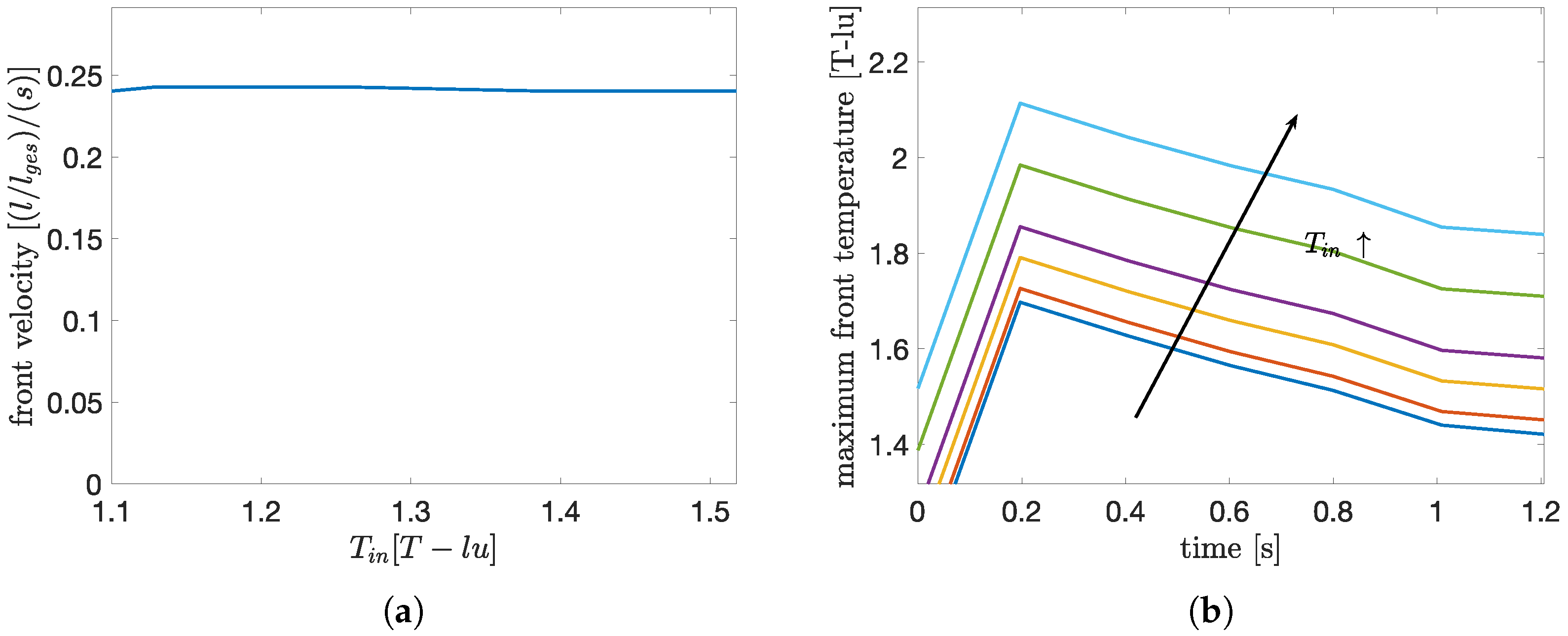
First, the Damköhler number, which is a measure of the ratio of the chemical reaction rate to the diffusive transport of the reactant, is varied. Since the initial simulation, which was shown in Figure 12, exhibited a transport-limited reaction for an inlet temperature of 1.5 T-lu, the range of values for the parametric study is chosen to be , corresponding to SI-unit values between 577 °C and 900 °C, which is equivalent to Damköhler numbers of . The results of the parametric study of the Damköhler number are shown in Figure 13, in which the maximum temperature of the combustion front over time and the propagation velocity of the combustion front are shown.
Figure 13.
Parametric study of Damköhler number: propagation velocity of the combustion front (a) and maximum temperature (b) for different inlet temperatures. In the graphs, the colors represent the following values of the inlet temperature : Tin = 1.1, Tin = 1.129, Tin = 1.19, Tin = 1.2857, Tin = 1.388, Tin = 1.5174. The arrow highlights the direction, in which the inlet temperature increases for this set of curves.
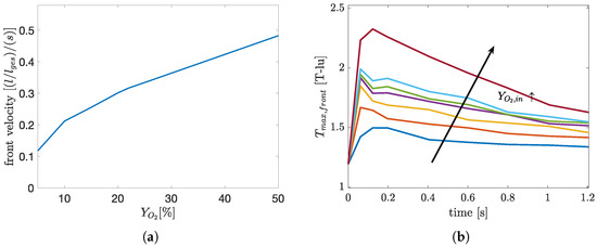
The time-averaged propagation velocity is calculated based on the position of the front for each Damköhler number. It can be seen that the profiles of the maximum temperature of the combustion front are similar, being just offset by the different values of the initial temperature. This indicates a transport-limited combustion regime with total turnover of the reactant provided at the inlet, even for inlet temperatures as low as 1.1 T-lu, corresponding to 577.3 °C. Thus, a further increase in the inlet temperature, resulting in higher reaction rates, does not result in a higher total release of reaction heat. Subsequently, the influence of the inlet mass fraction of oxygen on the reaction regime is investigated. Since a transport-limited combustion regime is identified for the given range of parameters, an increase in inlet mass fraction of oxygen, resulting in higher gradients, thus a higher mass transport, will have a greater effect on the combustion properties. Simulations are performed with a constant inlet temperature of 650 °C and for a range of and the results are shown in Figure 14.
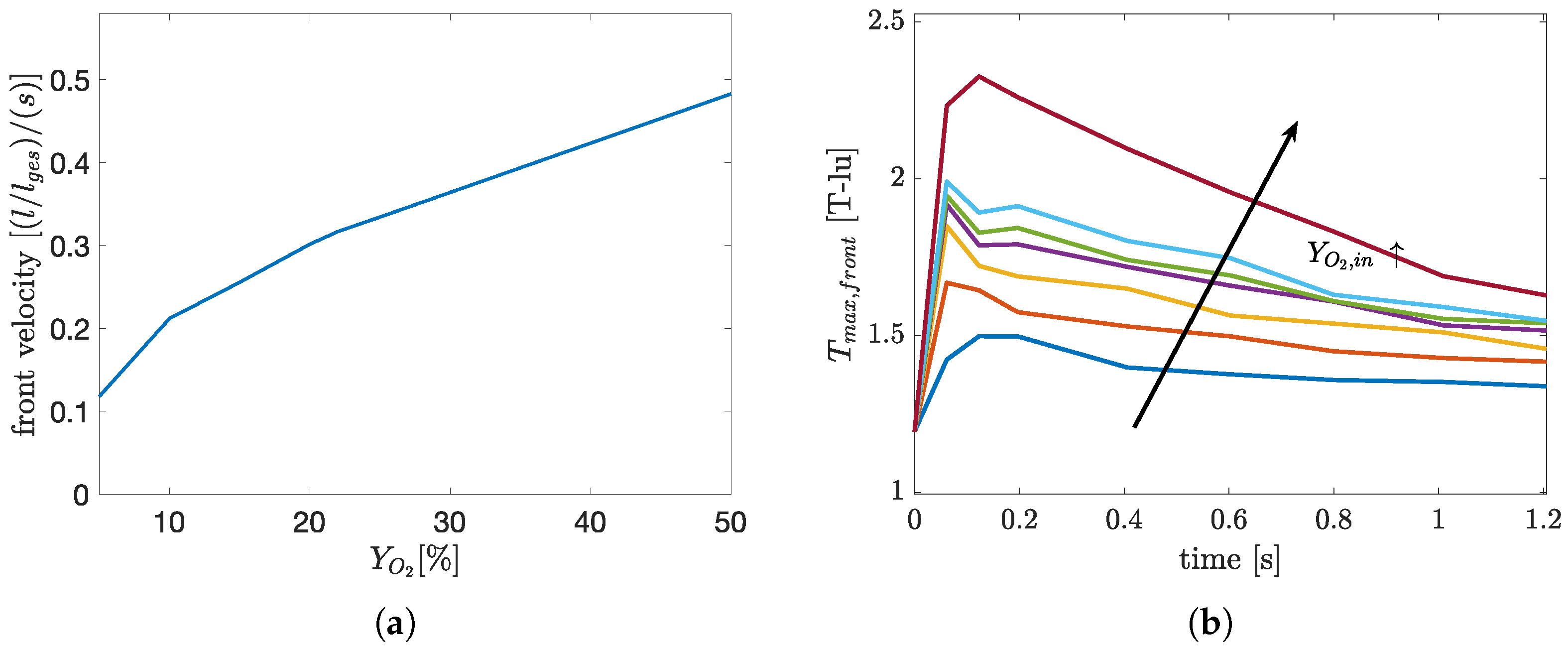
Figure 14.
Parametric study of : propagation velocity of the combustion front (a) and maximum temperature (b). In the graphs, the colors denote the following values of the inlet mass fraction of oxygen: YO2 = 5%, YO2 = 10%, YO2 = 5%, YO2 = 20%, YO2 = 22%, YO2 = 25%, YO2 = 50%. The arrow symbolizes the increase of inlet mass fraction of oxygen for the set of curves.
The temporal evolution of the combustion front position describes a similar course throughout the range of values of , resulting in an almost linear increase in the propagation speed, as can be seen in Figure 14a. The maximum front temperatures also exhibit similar profiles, with a maximum at 0.2 s, as shown in Figure 14b. This maximum is prominent for all values of . As expected for a transport-limited combustion regime, an increase in the provided reactant leads to a higher burn rate, resulting in a steeper drop in the residual coke mass. A value of results in approximately of the original coke mass being burned after 1.2 s, with resulting in a consumption of around and leading to a consumption of more than of the initial soot mass. Since all characteristic values, i.e., the velocity of the combustion front, the maximum front temperature and the consumption rate of coke, still change with an increase of , the combustion can still be assumed to take place in a transport-limited regime, even at inlet mass fractions of oxygen of .
Since an increase in the reactant mass fraction linearly increases the gradient of the mass fraction along the direction of the flow, which is the main driving force for mass transfer at , a linear dependency of the front velocity from the inlet reactant mass fraction should be presumed. As can be seen in Figure 14a, this assumption is fulfilled to a good degree. Subsequently, the influence of the Péclet number on the combustion mode is investigated. The Péclet number is varied by means of changing the inlet velocity and the results are shown in Figure 15, again with the propagation velocity and maximum temperature being displayed. More time steps are used for the evaluation of the simulation with Pe = 1 since the full conversion of the initial soot mass is achieved at .
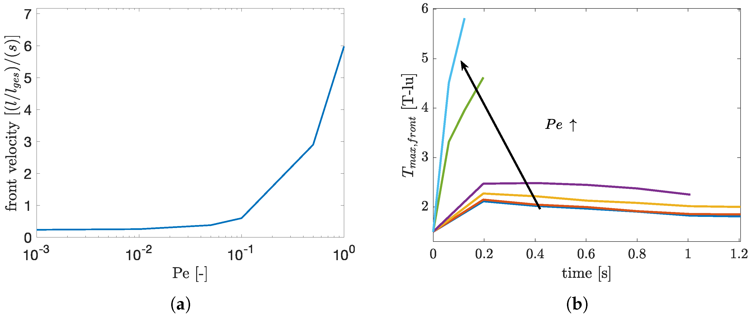
Figure 15.
Parametric Study Péclet number: propagation velocity of the combustion front (a) and maximum temperature (b) for different Péclet numbers (inlet velocities). Here, the colors represent the following Péclet numbers: Pe = 0.001, Pe = 0.01, Pe = 0.05, Pe = 0.1, Pe = 0.5, Pe = 1. The arrow symbolizes the direction, for which Pe increases in this set of curves.
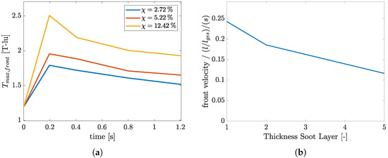
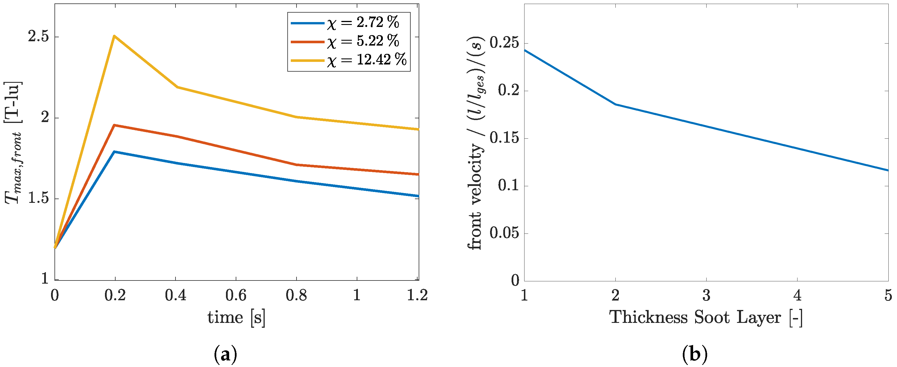
For a Péclet number of , the simulation reaches total conversion of soot after around . Further decreasing the Péclet number results in smaller changes in the temporal evolution of the residual coke mass in accordance with the fact that the advective transport becomes irrelevant. Furthermore, the propagation speed, displayed in the bottom left of Figure 15a, exhibits an exponential dependency of the Péclet number, and the maximum temperature of the combustion front shows a drastic increase to approximately 5.7 T-lu, compared to the range of 2–2.5 T-lu for . Both Pe and have an influence on the mass transport in the simulation. When comparing the propagation velocity for a change of Pe and of in the Figure 14a and Figure 15a, a different behavior can be noted. The propagation velocity for a change in shows a nearly linear dependency, also hinting an asymptotic behavior. This results from the driving force of mass transfer, in this specific case the gradient of , declining with propagation of the combustion front, dampening the effect of higher inlet mass fractions of oxygen. For , diffusion is the dominating phenomenon of mass transport. This results in an almost constant propagation velocity of the combustion front since the overall mass transport remains almost unchanged. For Péclet numbers approaching 1, the convective mass transport becomes relevant. This results in a steep incline in the front velocity due to the fact that the total mass transport drastically increases with further increases in the inlet velocity. Furthermore, the influence of the thickness of the reactive soot layer is investigated. For this purpose, the simulation domain is altered in such a way that the overall diameter of the round particles is kept constant, with the thickness of the outer reactive layer being altered. This leads to a change in the ratio of the reactive and inert solid masses while keeping the porosity of the system constant. Simulations are conducted with a layer thickness of one, two and five lattice nodes, with the first one being the standard case used in the previous parametric study. These soot layer thicknesses correspond to soot mass fractions of . The results of the study are shown in Figure 16, in which the maximum front temperature and the front velocity are shown. The simulations are performed with a Péclet number of 0.01, an inlet temperature of 1.19 T-lu, and an inlet mass fraction of oxygen of 0.2. It can be seen that the maximum front temperature increases with increasing soot layer thickness.
Figure 16.
Results of simulations with different thicknesses of the reactive soot layer. Shown are the maximum front temperature (a) and front velocity (b).
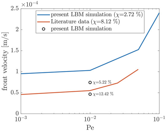
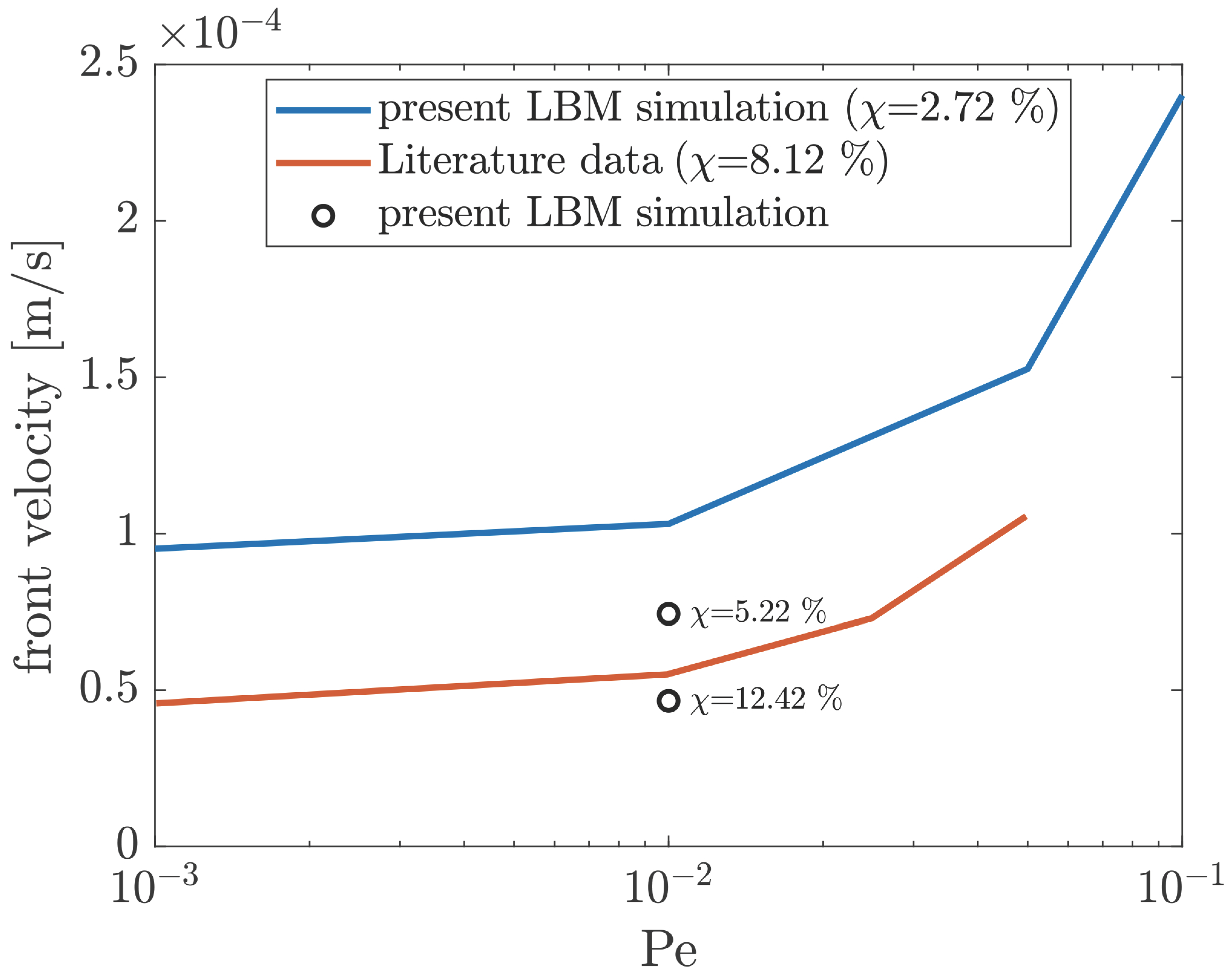
This results from the higher ratio of reactive to inert solid mass, which leads to a higher release of reactive energy compared to a smaller amount of inert, temperature-dampening mass. Furthermore, the higher amount of reactive mass per particle, in conjunction with the transport-limited combustion regime, results in a smaller front velocity for an increasing thickness of the soot layer. The transport-limited regime also equates to a different residual coke mass after a combustion simulation of . The oxygen provided at the inlet dictates the maximum reaction rate possible within the boundaries of the simulation. With more reactive soot initially present for higher soot layer thicknesses, the residual coke for a specific combustion time will increase accordingly. Subsequently, the results are compared to data published in [5]. Both our simulation and the results published in [5] are performed using the parameter set, shown in Table 1. Furthermore, the reaction mechanism used is the same in both cases. However, it has to be mentioned that the test case proposed in [5] consists of irregularly shaped particles while also employing a size distribution function. For the test case proposed here, spherical particles of uniform size were used. It is noted that the porosities and soot mass fractions are comparable in both cases. The literature data are shown in Figure 17 along the propagation speed of the combustion front, which was previously shown in Figure 15a. Additionally, the data points of Figure 16a are shown, as well for a qualitative comparison of the front velocities.
Figure 17.
Comparison of the front propagation velocity presented in [5] – and the simulation results presented here –.
Our simulations are performed at 500 °C, corresponding to a Damköhler number of , which equates the “relatively high Da” results of [5]. The previously discussed exponential increase in the combustion front propagation velocity, characteristic for the convection-dominated and reaction kinetics limited combustion regime, is prominent in both data sets, with the literature data only being available for Péclet numbers up to 0.05. The constant offset between our results and the literature results from the difference in soot mass fraction and porosity of the systems. Xu et al. [5] used a porous geometry based on glass beads with multimodal size distribution, a porosity of and a soot mass fraction of , while the simulation domain utilized here consisted of staggered spherical particles of uniform size, with a porosity of and a soot volume fraction of . As was shown in Figure 16b, an increase in the soot volume fraction results in a slower combustion front. The reaction-kinetics-limited combustion regime implies a constant solid conversion rate. Increasing the solid mass fraction of the simulation domain thus results in longer necessary burn-off times and lower combustion speeds. This can be visualized by adding the data shown in Figure 16b as data points to Figure 17. It becomes apparent that the data of [5] lies in between the simulations performed for and , indicating good congruence, even though the geometry presented in [5] consists of irregularly formed particles, rather than perfect spheres.
5.3. CO-CO2 Pathways—Comparison with Experimental Data
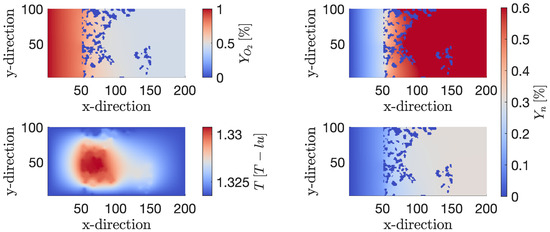
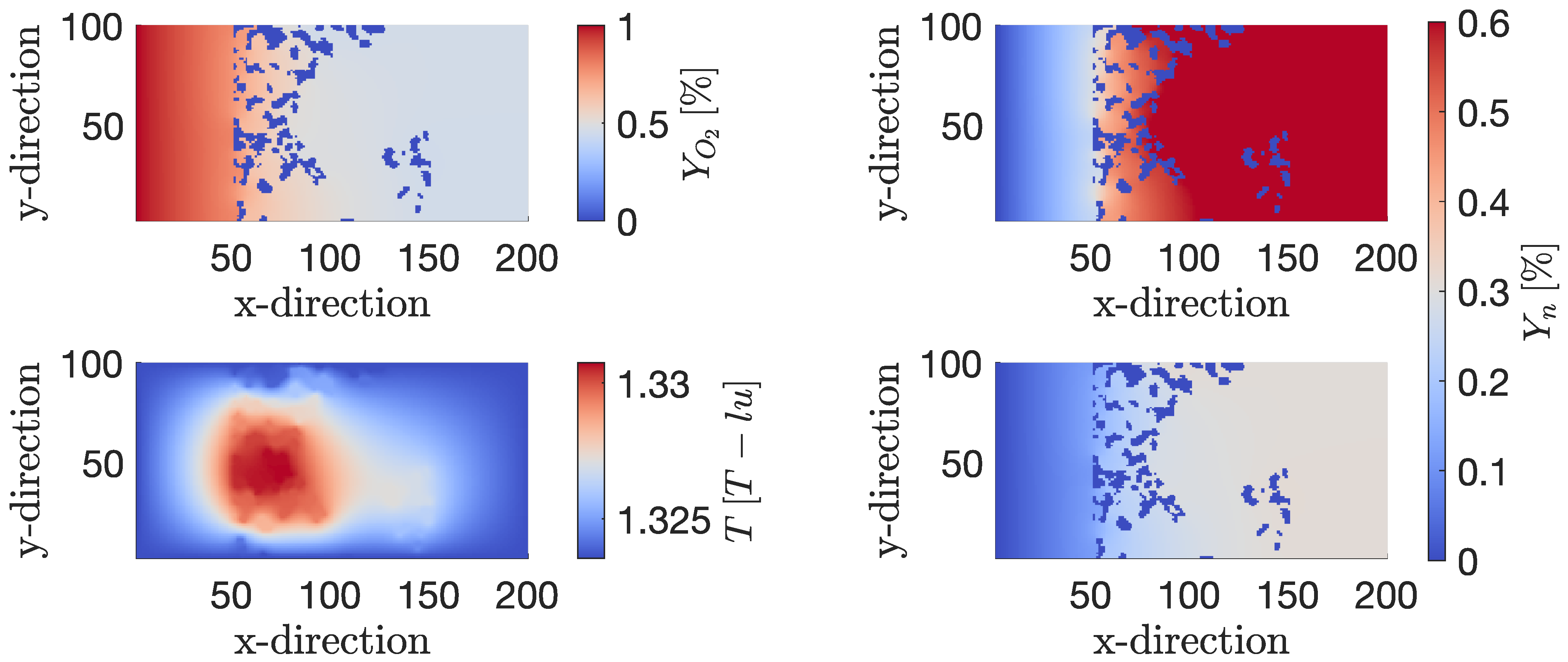
Furthermore, the influence of temperature on the CO and CO2 reaction pathways was studied by comparing LBM simulations with experimental data. A detailed description of the experimental setup can be found in [28]. In the combustion experiments, the two components CO and CO2 in the outlet gas stream are quantified using a mass spectrometer. For the reaction kinetics, values for the activation energy of kJ/mol and kJ/mol are used for the CO2 and CO pathways [28]. Then, combustion simulations at different temperatures are performed. Since the ratio of is temperature dependent, the combustion simulations are set up with non-adiabatic walls at the top and bottom to mitigate the influence of the reaction heat, which is released during the simulation. Furthermore, small inlet mass fractions of O2 are used to further decrease the influence of the reaction heat. The resulting steady state solution for an inlet temperature of 750 °C with an inlet velocity of m/s, similar to the parameters used in the experiments and with an inlet mass fraction of O2 of , is shown in Figure 18.
Figure 18.
Steady-state solution of the mass fraction of oxygen (top left), CO (top right), temperature (bottom left) and CO2 (bottom right) for an inlet temperature of 750 °C and .
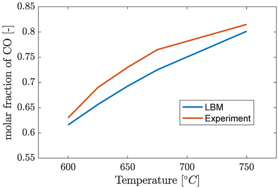
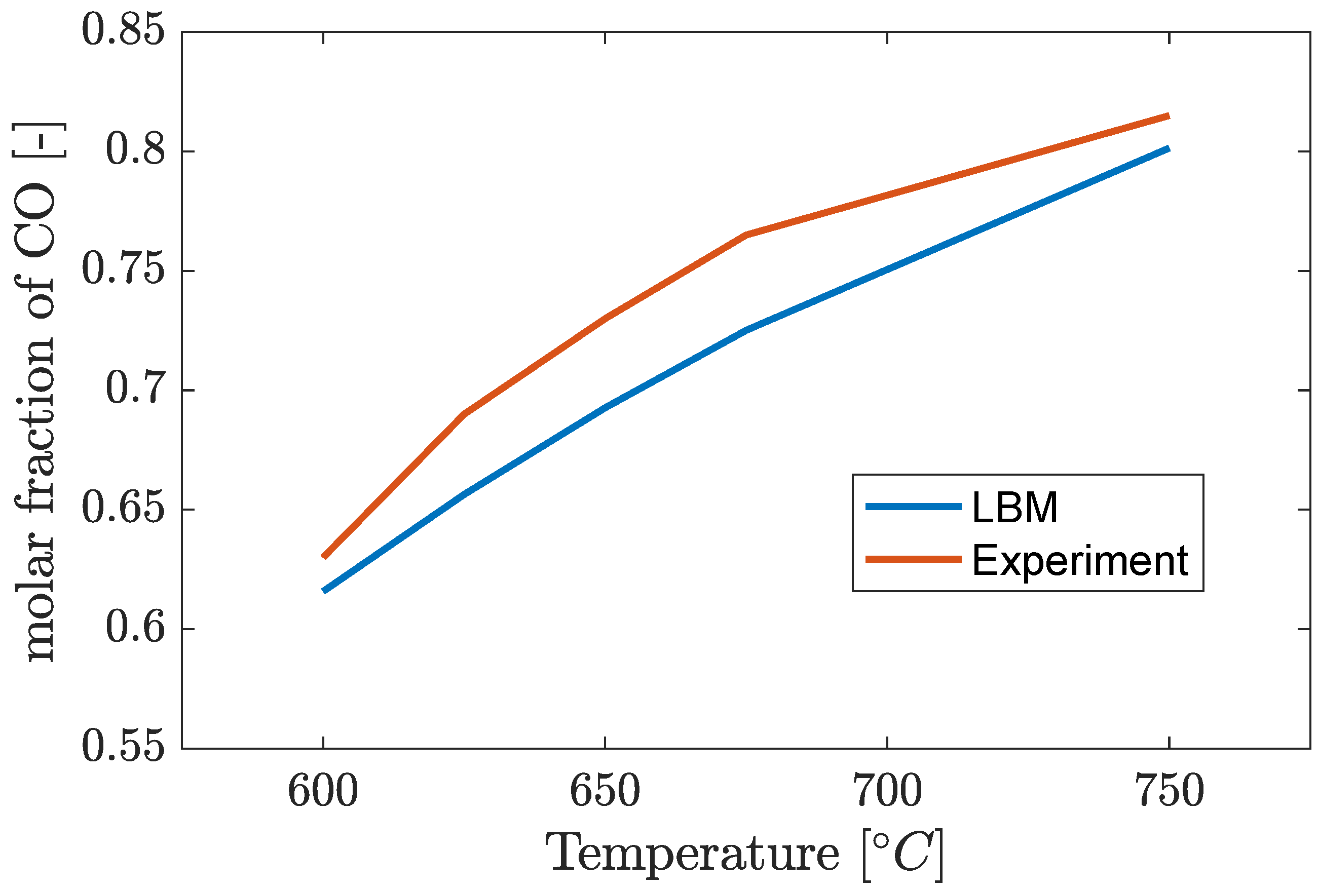
On the left, the mass fraction of the educt O2 and the temperature in lattice units are shown. On the right, the mass fractions of CO and CO2 are shown on the top and bottom, respectively. A slight temperature increase can be observed in the center of the domain, equating to approximately 4 °C. The temperature profile reaches a steady state when the reaction heat, produced by the combustion reaction, and the heat flux through the boundaries, which are kept at a constant temperature, are equivalent. With this steady-state temperature profile, the combustion consumes approximately half of the oxygen, which is provided to the computational domain at the inlet. Furthermore, it can be observed that around of the total consumed oxygen is consumed by the partial reaction forming CO, as can be seen on the right. Further simulations are performed for inlet temperatures between 600 °C and 750 °C, in accordance with the experimental investigation. The resulting mass fractions of CO and CO2 at the outlet are converted to molar fractions for comparison with the measurements of the mass spectrometer. The resulting molar fraction of CO, with reference to the total molarity of CO and CO2, is shown in Figure 19. Since the activation energy of the partial oxidation reaction of carbon is higher than the activation energy for the full oxidation to CO2, it is expected that the molar fraction of CO increases for increasing temperatures [29]. This behavior is reproduced by both the experimental data, shown in red, and the results of the simulation, shown in blue. At 600 °C, the combustion experiment shows a molar ratio of , with the LBM simulation resulting in . The difference between the experimental data and the LBM simulations remains mostly constant with deviations between 2 and 4% pt. At 750 °C, the LBM and experimental data result in and , respectively.
Figure 19.
Molar fraction of CO with respect to the molarity of CO and CO2.
6. Conclusions
In the present paper, the formulation and implementation of boundary conditions and algorithms for the description of heterogeneous reactions with the lattice Boltzmann method have been shown. Furthermore, the model was extended to 3D and validated following the same procedure as that for the validation of the 2D model. A breath-first search algorithm was implemented to calculate the accessible reactive surface. The BFS was implemented in a parallel manner, resulting in performance gains of a factor of six, reducing the performance overhead significantly. Moreover, the combustion behavior of a regular two-dimensional domain consisting of round inert particles, coated with reactive soot, was investigated. This was achieved by the systematic variation of the characteristic variables of the Péclet number, the Damköhler number and the inlet mass fraction of oxygen . The model has proven its capability to capture the expected dependencies of the propagation velocity of the combustion front, namely a linear dependency of , as well as an exponential dependency of Pe in the case of transport-limited combustion. Additionally, the comparison of the ratio obtained by LBM for different temperatures with experimental data showed good model accuracy in the range of 2–4% pt.
This was done in preparation for our further efforts to study the influence of the soot morphology on the reaction rate and to investigate the evolution of the reactive surface with the propagating reaction.
Author Contributions
Conceptualization, C.S. and M.S.S.; methodology, C.S. and M.S.S.; software, C.S.; validation, C.S. and A.R.; formal analysis, C.S.; investigation, C.S.; resources, C.S.; data curation, C.S.; writing—original draft preparation, C.S.; writing—review and editing, C.S., A.R., A.H., U.N. and M.S.S.; visualization, C.S.; supervision, M.S.S., U.N. and A.H.; project administration, U.N., A.H. and M.S.S.; funding acquisition, U.N., A.H. and M.S.S. All authors have read and agreed to the published version of the manuscript.
Funding
Our thanks go to the German Research Foundation (DFG) and the Agence Nationale de la Recherche (ANR) for financial support with grant number NI 932/17–1 and ANR-20-CE92-0007.
Data Availability Statement
Data will be made available upon reasonable request.
Conflicts of Interest
The authors declare that they have no known competing financial interests or personal relationships that could have appeared to influence the work reported in this paper.
Abbreviations
The following abbreviations are used in this manuscript:
| CO | Carbon monoxide |
| CO2 | Carbon dioxide |
| Da | Damköhler number |
| FIB-SEM | Focused ion beam scanning electron microscopy |
| ICVT | Institute of Chemical Process Engineering |
| LBM | Lattice Boltzmann method |
| LB | Lattice Boltzmann |
| MRT | Multi relaxation time |
| O2 | Oxygen |
| Pe | Péclet number |
| RMS | Root mean square error |
| SRT | Single relaxation time |
Appendix A. 3D Soot Sample
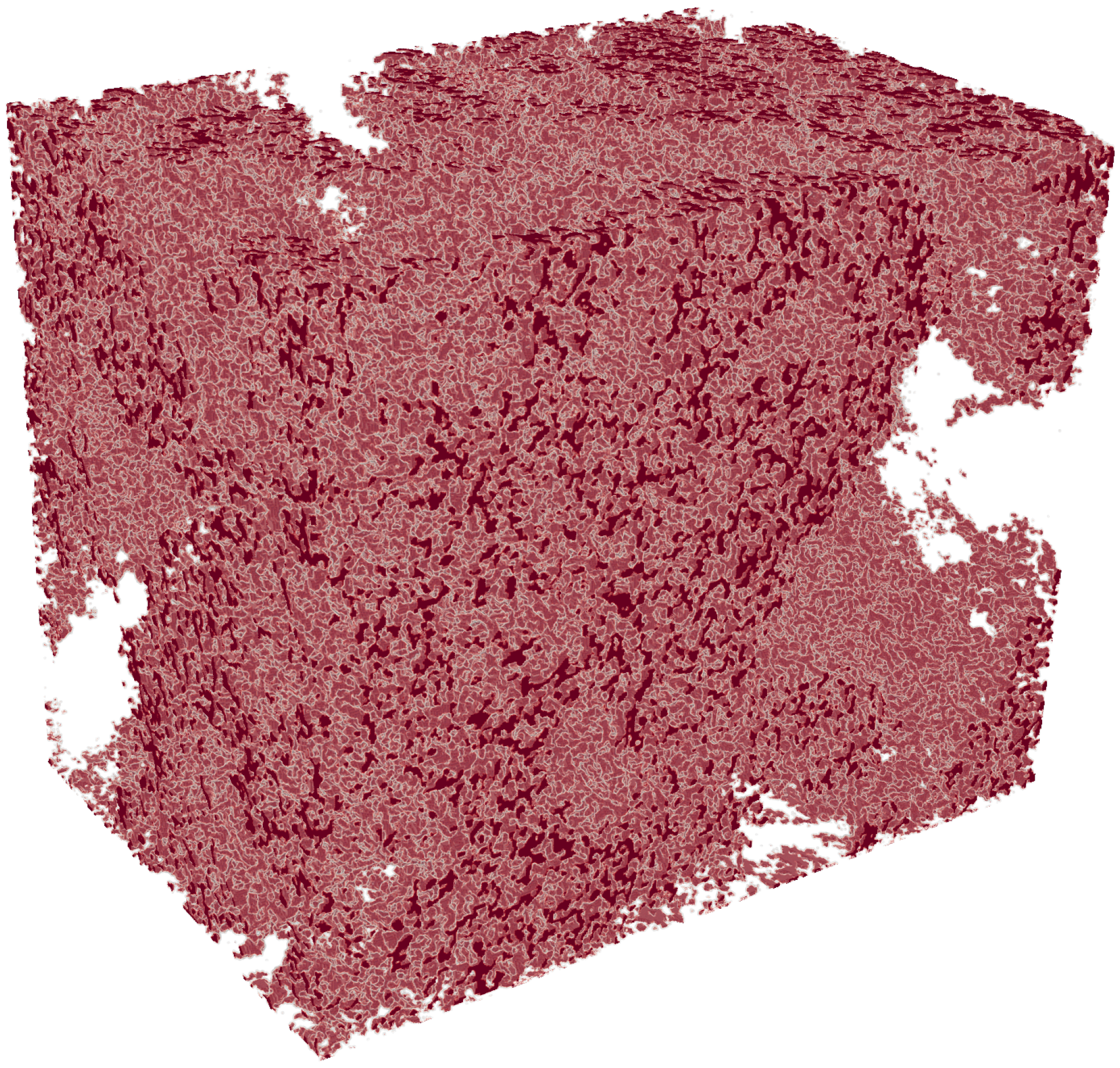
In Figure A1, the 3D soot domain, obtained by the FIB-SEM analysis of soot samples obtained with a combustion aerosol standard (CAST) soot generator, is shown.
Figure A1.
3D reconstruction of FIB-SEM data of a real soot sample.
Appendix B. Breadth First Search Algorithm
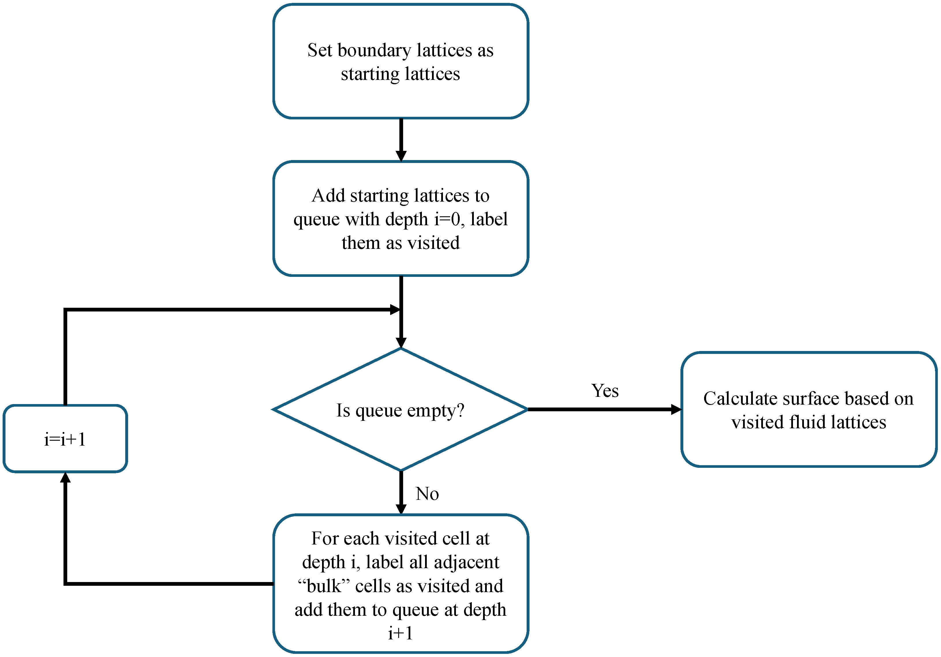
The basic principle of the calculation of the accessible reactive surface is visualized in the following flowchart, given in Figure A2:
First, the boundary lattice nodes of the domain are set as starting nodes and, thus, added to the queue at depth and labeled as visited. Then, the algorithm propagates through the queue. The neighbors of each lattice node, which is inside of the queue at the current depth, i, are analyzed regarding their property. If the property is set to be bulk (here, the flag for a gas-phase node), then the lattice is added to the queue at the depth of and marked as visited. As such, the algorithm propagates until the queue is empty. Then, all “accessible” lattice nodes are marked as visited. Based on this marker, the surface accessible by reactants, the true reactive surface, can be calculated by searching for bulk-solid neighboring pairs, in which the bulk cell has been visited.
Figure A2.
Flowchart of the BFS algorithm.
The algorithm is implemented by utilizing two vectors, one of type “std::vector visited”, in which the information, if a cell has been “visited” by the algorithm, is stored as a Boolean variable (true or false). The second vector is of type “std::queue q”, which saves the index of the visited cells. The algorithm starts by assigning the outermost nodes of the domain to the queue-vector by utilizing the c++ command “push”. This adds the pushed cell to the top of the queue. Also, the cells are marked as “true” in the Boolean vector. This is done because the outermost nodes are used as a starting point to propagate through the domain and to find all accessible gaseous nodes. Then, a while-loop is performed with the condition “!q.empty”, which means that the following operators will be executed as long as there are cells left inside of the queue-vector q. Inside of the while-loop, the uppermost index stored in vector q is taken. Subsequently, its four neighboring nodes are being examined according to “celltype::bulk” “!visited”, which means that they are assigned to the gas phase and have not yet been visited. If this condition is true, the neighboring node is added to the list q, and its Boolean value is set to “true”. Since a while-loop is used, the algorithm will propagate through the part of the domain, which is of type gas-phase and connected with the outer flow. Explicitly, it would mean that the inner cavity, as shown in Figure 4, would be excluded by the algorithm. Finally, after the code leaves the while-loop, a for-loop is executed, which runs over all cells of the domain. Inside, with an if-condition, the cells assigned to the solid-domain are taken, and their neighbors are examined. If the neighbor is of type “gas-phase” and has been “visited” by the previous search algorithm, then the value of the surface is increased by the value of 1 lattice spacing.
| Algorithm A1 Breadth-First Search and Surface Calculation |
|
Appendix C. Relaxation Parameters and Collision Operators
In the following, the transformation matrix M, as well as the relaxation matrices S, and , are defined. The transformation matrix M, which is used to perform collision in moment space, rather than lattice space, is given as:
The relaxation matrix S for the velocity field is given by:
Here, the order of the rows of the matrices M and S depends on the chosen lattice discretization and order of lattice velocity vectors, which can be chosen arbitrarily. The matrices that are shown here correspond to the D2Q9 lattice velocity set with the ordering, which is shown in Figure 1. The entries , and are parameters, which can be chosen by the user, while is defined by the physics of the problem. Following the Chapman–Enskog expansion, is linked to the kinematic viscosity by the following relation:
A good explanation of the Chapman–Enskog expansion and the derived closure condition can be found in [30]. When simulating cases with negligible diffusion and high advection, meaning , the parameters and can be tuned to mitigate the effect of truncation errors, thus reducing the effect of numerical diffusion. Also, relates to third-order moments, meaning that a smart choice of can decrease the effects of lattice anisotropy.
Similarly, the relaxation matrices for the temperature field and component fields, and are defined. The only distinction is the substitution of the term relating to momentum diffusion, by and .
Appendix D. Mesh Sensitivity Analysis
When performing simulations with LBM, performing mesh sensitivity analysis is imperative, similar to other discretization methods of partial differential equations. However, since the simulations are performed in lattice units, the conversion factor from SI-units to lattice units changes when the lattice spacing is altered. For this reason, the conversion of all variables and parameters has to be performed for each lattice spacing independently. A full description of the conversion procedure can be found in [18].
The goal of performing mesh sensitivity analysis, also known as grid convergence, is to identify a mesh spacing which is sufficient to resolve the physics of the given test case while keeping the computational effort as low as possible. Simulations are performed with different lattice resolutions, and characteristic variables are compared between the different mesh sizes. For the given combustion test case shown in this paper, grid convergency was performed with lattice spacings of 0.5 μm, 1 μm and 2 μm. In Figure A3, the results of the mesh sensitivity analysis are shown. In Figure A3a, the y-velocity profile, and in Figure A3b, the temperature profile along the symmetry line of the domain is shown for a simulation time of 12 ms.
Figure A3.
Profile of y-velocity (a) and temperature (b) along the symmetry line of the combustion test case for lattice spacings of 0.5 μm, 1 μm and 2 μm.
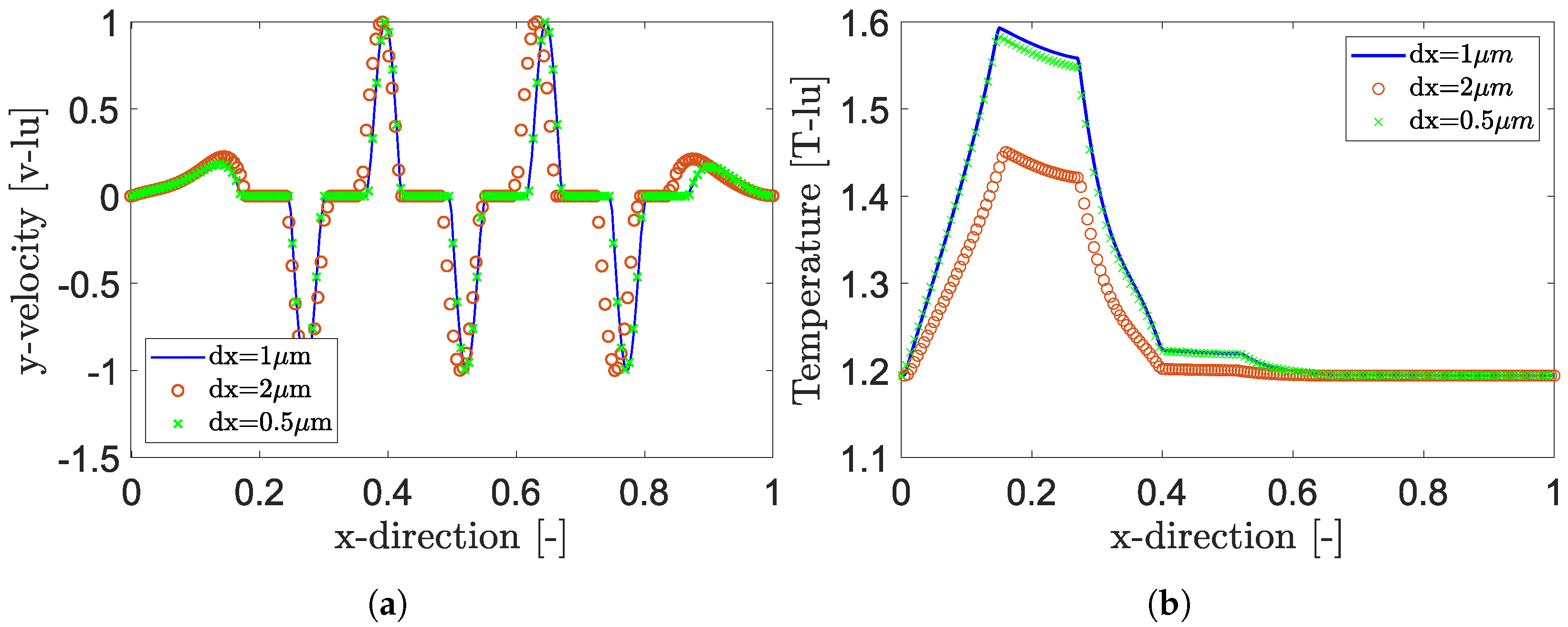
It can be seen that a lattice spacing of 2 μm is not sufficient to accurately resolve the physics of the test case, while the lattice spacing of 1 μm closely resembles the result for a spacing of 0.5 μm while resulting in drastically decreased computational effort. The gain in performance is not only attributed to the reduced lattice count but also results from the increased time-step size, which is received from the closure condition of the Chapman–Enskog expansion. In conclusion, for the given test cases shown in this manuscript, a lattice spacing of has been chosen. This is in line with the discretization width presented in [5,7].
Appendix E. Conversion from SI-Units to Lattice Units
For the conversion of parameters from SI-units to lattice units, conversion factors for all base units have to be defined. For the given case of simulating heterogeneous reactions in porous media, these include time s, space m, mass kg, temperature K and molarity mol. In a first instance, the lattice size in SI-units is chosen based on the given test case. Then, the time discretization is received from the closure condition, originating from the Chapman–Enskog expansion:
In LBM, it is common to define and in lattice units. Thus, the conversion factors for space and time are received as:
Moreover, the density in lattice units is always set as , meaning that the mass conversion factor is received implicitly from and the given density of the test case as:
Finally, the conversion factors for temperature and molarity are received by defining reference values, i.e., the initial temperature and the molar mass of a specific component:
and:
References
- Jurtz, N.; Kraume, M.; Wehinger, G.D. Advances in fixed-bed reactor modeling using particle-resolved computational fluid dynamics (CFD). Rev. Chem. Eng. 2019, 35, 139–190. [Google Scholar] [CrossRef] [Scilit]
- McLaren, A.D. Temporal and Vectorial Reactions of Nitrogen in Soil: A Review. Can. J. Soil Sci. 1970, 50, 97–109. [Google Scholar] [CrossRef] [Scilit]
- Fattahi, E.; Waluga, C.; Wohlmuth, B.; Rüde, U.; Manhart, M.; Helmig, R. Lattice Boltzmann methods in porous media simulations: From laminar to turbulent flow. Comput. Fluids 2016, 140, 247–259. [Google Scholar] [CrossRef] [Scilit]
- Sadeghi, R.; Shadloo, M.S.; Hopp-Hirschler, M.; Hadjadj, A.; Nieken, U. Three-dimensional lattice Boltzmann simulations of high density ratio two-phase flows in porous media. Comput. Math. Appl. 2018, 75, 2445–2465. [Google Scholar] [CrossRef] [Scilit]
- Xu, Q.; Long, W.; Jiang, H.; Zan, C.; Huang, J.; Chen, X.; Shi, L. Pore-scale modelling of the coupled thermal and reactive flow at the combustion front during crude oil in-situ combustion. Chem. Eng. J. 2018, 350, 776–790. [Google Scholar] [CrossRef] [Scilit]
- Yamamoto, K.; Sakai, T. Simulation of continuously regenerating trap with catalyzed DPF. Catal. Today 2015, 242, 357–362. [Google Scholar] [CrossRef] [Scilit]
- Lei, T.; Wang, Z.; Luo, K.H. Study of pore-scale coke combustion in porous media using lattice Boltzmann method. Combust. Flame 2021, 225, 104–119. [Google Scholar] [CrossRef] [Scilit]
- Guo, B.; Xu, H.J.; Zhao, C.Y. Lattice Boltzmann modelling on pore-scale reactive transport in exothermic reactions of solid blocks for thermochemical energy storage. Appl. Therm. Eng. 2022, 216, 119145. [Google Scholar] [CrossRef] [Scilit]
- Wang, M.; Zhu, W. Pore-scale study of heterogeneous chemical reaction for ablation of carbon fibers using the lattice Boltzmann method. Int. J. Heat Mass Transf. 2018, 126, 1222–1239. [Google Scholar] [CrossRef] [Scilit]
- Yang, X.; Zhan, C.; Liu, X.; Chai, Z. A diffuse-interface lattice Boltzmann method for the dissolution through nonlinear heterogeneous reaction. Phys. Fluids 2025, 37, 053306. [Google Scholar] [CrossRef] [Scilit]
- Wei, X.; Li, W.; Liu, Q.; Sun, W.; Liu, S.; Li, S.; Wei, H.; Ma, L. Pore-scale investigation on multiphase reactive transport for the conversion of levulinic acid to γ-valerolactone with Ru/C catalyst. Chem. Eng. J. 2022, 427, 130917. [Google Scholar] [CrossRef] [Scilit]
- Hao, H.; Xu, Z.G. Pore-scale investigation on dissolution and precipitation considering secondary reaction in porous media by LBM. Gas Sci. Eng. 2023, 110, 204893. [Google Scholar] [CrossRef] [Scilit]
- Mishra, S.K.; De, A. Coupling of reaction and hydrodynamics around a reacting block modeled by Lattice Boltzmann Method (LBM). Comput. Fluids 2013, 71, 91–97. [Google Scholar] [CrossRef] [Scilit]
- Abdollahzadeh, Y.; Mansourpour, Z.; Moqtaderi, H.; Ajayebi, S.N.; Montazeri, M.M. A molecular collision based Lattice Boltzmann method for simulation of homogeneous and heterogeneous reactions. Chem. Eng. Res. Des. 2018, 136, 456–467. [Google Scholar] [CrossRef] [Scilit]
- Kang, Q.; Lichtner, P.C.; Janecky, D.R. Lattice boltzmann method for reacting flows in porous media. Adv. Appl. Math. Mech. 2010, 2, 545–563. [Google Scholar] [CrossRef] [Scilit]
- Karani, H.; Huber, C. Lattice Boltzmann formulation for conjugate heat transfer in heterogeneous media. Phys. Rev. E—Stat. Nonlinear Soft Matter Phys. 2015, 91, 023304. [Google Scholar] [CrossRef] [Scilit]
- Li, L.; Chen, C.; Mei, R.; Klausner, J.F. Conjugate heat and mass transfer in the lattice Boltzmann equation method. Phys. Rev. E—Stat. Nonlinear Soft Matter Phys. 2014, 89, 043308. [Google Scholar] [CrossRef] [Scilit] [PubMed]
- Stockinger, C.; Raiolo, A.; Alamian, R.; Hadjadj, A.; Nieken, U.; Shadloo, M.S. Lattice Boltzmann simulations of heterogeneous combustion reactions for application in porous media. Eng. Anal. Bound. Elem. 2024, 166, 105817. [Google Scholar] [CrossRef] [Scilit]
- Stockinger, C. Study and Analysis of Soot Filter Regeneration by Using the Lattice Boltzmann Method. Ph.D. Thesis, Insa Rouen Normandie, Rouen, France, 2024. [Google Scholar]
- Mailybaev, A.A.; Bruining, J.; Marchesin, D. Analysis of in situ combustion of oil with pyrolysis and vaporization. Combust. Flame 2011, 158, 1097–1108. [Google Scholar] [CrossRef] [Scilit]
- Qian, Y.H.; D’Humières, D.; Lallemand, P. Lattice bgk models for navier-stokes equation. EPL 1992, 17, 479–484. [Google Scholar] [CrossRef] [Scilit]
- Guo, Z.; Zheng, C.; Shi, B. Discrete lattice effects on the forcing term in the lattice Boltzmann method. Phys. Rev. E—Stat. Phys. Plasmas Fluids Relat. Interdiscip. Top. 2002, 65, 046308. [Google Scholar] [CrossRef] [Scilit]
- Frisch, U.; Hasslacher, B.; Pomeau, Y. Lattice-gas automata for the Navier-Stokes equation. Phys. Rev. Lett. 1986, 56, 1505–1508. [Google Scholar] [CrossRef] [Scilit] [PubMed]
- Ginzburg, I.; Roux, L.; Silva, G. Local boundary reflections in lattice Boltzmann schemes: Spurious boundary layers and their impact on the velocity, diffusion and dispersion. Comptes Rendus Méc. 2015, 343, 518–532. [Google Scholar] [CrossRef] [Scilit]
- Ginzburg, I. Generic boundary conditions for lattice Boltzmann models and their application to advection and anisotropic dispersion equations. Adv. Water Resour. 2005, 28, 1196–1216. [Google Scholar] [CrossRef] [Scilit]
- Ho, C.F.; Chang, C.; Lin, K.H.; Lin, C.A. Consistent boundary conditions for 2D and 3D lattice boltzmann simulations. Comput. Model. Eng. Sci. 2009, 44, 137–155. [Google Scholar]
- Zuse, K. Über den Allgemeinen Plankalkül als Mittel zur Formulierung schematisch-kombinativer Aufgaben. Arch. Math. 1948, 1, 96–105. [Google Scholar] [CrossRef] [Scilit]
- Raiolo, A.; Stockinger, C.; Tuttlies, U.; Ivleva, N.P.; Shadloo, M.S.; Nieken, U. Effect of nanostructure and BET surface area on the oxygen reactivity of soot filter cakes. Carbon 2024, 227, 119251. [Google Scholar] [CrossRef] [Scilit]
- Du, Z.; Sarofim, A.F.; Longwell, J.P.; Tognotti, L. The CO/CO2 Ratio in the Products of the Carbon-Oxygen Reaction. In Fundamental Issues in Control of Carbon Gasification Reactivity; Springer: Dordrecht, The Netherlands, 1991; pp. 91–106. [Google Scholar] [CrossRef] [Scilit]
- Kruger, T.; Kusumaatmaja, H.; Kuzmin, A.; Shardt, O.; Goncalo, S.; Viggen, E.M. The Lattice Boltzmann Method, Principles and Practice; Springer International Publishing: Cham, Switzerland, 2017; pp. 1–705. [Google Scholar]



Disclaimer/Publisher’s Note: The statements, opinions and data contained in all publications are solely those of the individual author(s) and contributor(s) and not of MDPI and/or the editor(s). MDPI and/or the editor(s) disclaim responsibility for any injury to people or property resulting from any ideas, methods, instructions or products referred to in the content. |
© 2026 by the authors. Licensee MDPI, Basel, Switzerland. This article is an open access article distributed under the terms and conditions of the Creative Commons Attribution (CC BY) license.