Comprehensive Dataset of Unidirectional Carbon Fiber Pultruded Composites and Their Constituents (Fibers and Matrix)

Abstract

A comprehensive experimental dataset for unidirectional carbon fiber pultruded composites is presented, including mechanical testing results, microscopy images, and X-ray computed tomography volumes. In contrast to typical datasets, all measurements consistently describe a single material system, encompassing both the composite and its constituents (carbon fibers and vinyl ester matrix), thereby enabling a comprehensive and coherent multiscale material characterization. X-ray-computed tomography images of samples extracted from three pultruded composite profiles were acquired with a voxel size of 0.55 µm and analyzed to determine the fiber orientation distribution. Scanning electron microscopy with a pixel size of 0.098 µm was used to determine the overall and local fiber volume fractions. Compression testing of 17 composite specimens provided the compressive properties. The tensile and shear properties of the matrix were obtained from tensile and shear tests on seven and four matrix specimens, respectively. The Ramberg-Osgood model was fitted to the matrix’s tensile stress–strain response. Single-fiber tensile testing was conducted on 255 carbon fibers with three gauge lengths to determine fiber properties and Weibull parameters. All mechanical tests were performed up to material failure. The dataset is suitable for semi-analytical predictions and numerical finite-element modeling of composite mechanical behavior.

Dataset: https://doi.org/10.5281/zenodo.18435237 (accessed on 26 January 2026), https://doi.org/10.5281/zenodo.18364215 (accessed on 26 January 2026), https://doi.org/10.5281/zenodo.18370051 (accessed on 26 January 2026), https://doi.org/10.5281/zenodo.18364338 (accessed on 26 January 2026).

Dataset License: CC BY 4.0

1. Summary

X-ray-computed tomography (CT) scanning is widely used to conduct a variety of analyses of fiber-reinforced composite materials [1,2,3]. These analyses, in most cases, require additional material data from both the composite and its constituents, namely the fibers and the matrix. Although many researchers have thoroughly characterized the mechanical properties of composite materials [4,5,6,7], comprehensive datasets that consistently describe a single material system, including both the composite and its constituents, are often not available. This limits the ability to perform fully consistent material characterization and numerical modeling.

This work aims to address this gap by acquiring the material data required for a full description of the single material system of a unidirectional pultruded composite and its constituents. The presented dataset provides detailed information on the composite material and its components (fiber and matrix) by combining experimental and post-processing data, which can then be reused for material characterization studies, allowing for multi-scale material characterization and reuse in a wide range of studies. To characterize the fibers, single-fiber tensile tests were conducted at three gauge lengths: 30 mm, 50 mm, and 70 mm. In total, 255 single fibers were tested, taken from different lengths of the studied tow. The roving of the examined carbon fibers had a single fiber count of 50,000 per yarn. The vibroscope method was used to measure single-fiber diameter, and a statistical analysis of the single-fiber filaments was performed using the Weibull model, as proposed by Kumar et al. [8].

The vinyl ester matrix material characterization included tensile and shear tests performed on samples cut from a cured pure resin plate. Seven matrix samples were subjected to tensile testing, while four were used for shear tests. For describing the matrix’s stress–strain behavior, particularly for FEM applications, the Ramberg–Osgood material model can be used, as it captures the matrix’s nonlinear strain-hardening behavior [9]. Therefore, the Ramberg–Osgood material model parameters for the matrix were identified in this work.

Seventeen composite samples were subjected to compression testing, cut from three unidirectional, carbon fiber-reinforced, pultruded profiles. Two groups of six samples and one of five were used, with each group corresponding to one profile. The three pultruded profiles were manufactured from the same base material; however, small, intended variations in pultrusion process parameters resulted in slight differences among the sample groups. Thirteen specimens were cut from the pultruded profiles to be used for the burn-off method and subsequent experimental determination of the fiber volume fraction. In addition, the fiber volume fraction was also determined using scanning electron microscopy (SEM), according to the method described by Mikkelsen et al. [10].

X-ray CT scanning was conducted on three composite samples at the DanMAX beamline at the MAX IV synchrotron facility. Each sample was cut from one of the three pultruded profiles from which the compression testing specimens were derived. The resulting data, with a voxel size of 0.55 μm, were used to acquire the fiber orientation distribution via structure tensor analysis, an image analysis method applied to volumetric data [11,12].

This dataset has been used as input for numerical modeling by Mageira et al. [13,14,15], where the X-ray CT scans of the three samples presented here, along with most of the acquired material data, were used as input for a built finite element model. This model employed material homogenization and was subjected to compression. The results focused on a numerical compressive-strength prediction of the material, accounting for the composite’s fiber orientation distributions.

By including detailed measurements of the fiber orientation distribution for microstructural analysis, as well as X-ray CT scans of the composite, the presented dataset can be reused for image analysis, 3D reconstruction, or algorithm development. Additionally, it contains the mechanical properties of both the composite and its constituents, making it suitable for comparative studies and multi-scale numerical modeling. The dataset is available on the Zenodo repositories. Specifically, the X-ray CT scans of the samples are provided in [16,17,18], while the repository containing all material data, analyses, and characterization presented in this work is available in [19]. The dataset serves as the basis for ongoing research within the EU Horizon RELIANCE consortium, supporting 13 PhD projects focused on modeling and characterizing composite materials.

2. Data Description

2.1. Fibers

2.1.1. Fiber Diameter Distribution

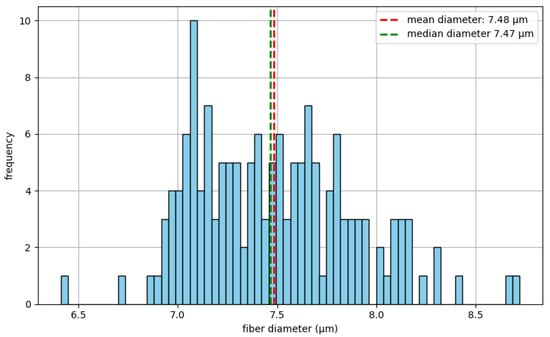
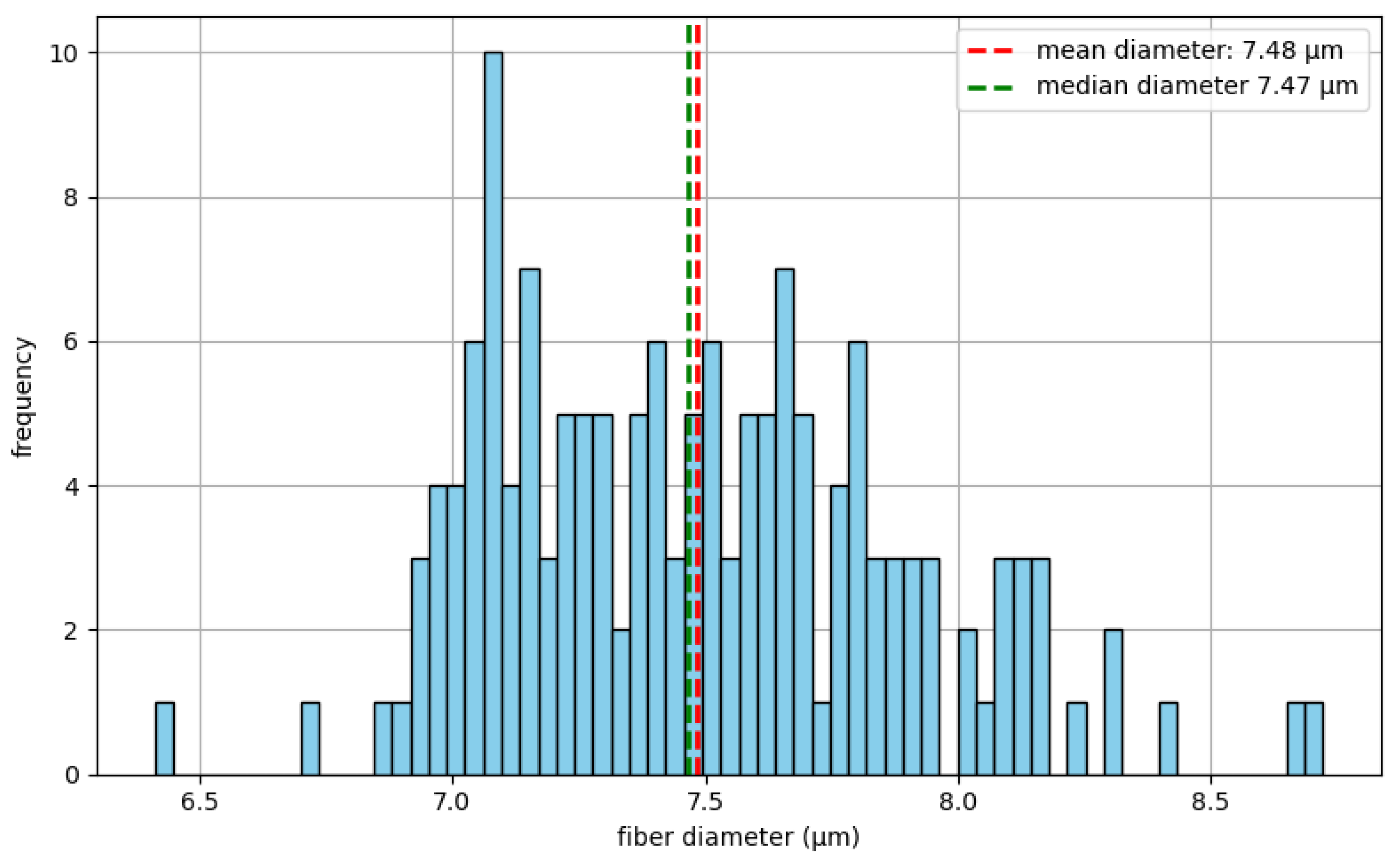
Figure 1 illustrates the distribution of the fiber diameter. It must be noted that in this work, the term fiber corresponds to what is considered a carbon filament, as it is widely used in similar articles [20]. The cross-section of a carbon fiber is kidney-shaped [21,22]. Still, to quantify and distribute the results of the size of the fiber cross-sectional area, an equivalent circle area was considered, from which the fiber diameter was derived. The calculation process and the applied methodology are described in detail in Section 3.1.1. The number of tested fibers was 154 (gauge length of 50 mm), with a mean diameter of 7.48 μm, a median diameter of 7.47 μm, and a standard deviation of 0.41 μm. The histogram peak corresponds to the most frequent diameter range, 7.10 µm. The close values of the mean and the median diameters, along with the relatively small standard deviation, indicate a narrow and approximately symmetric distribution. Therefore, the mean and median are considered representative. The obtained carbon fiber diameter is consistent with values reported in the literature, which are typically in the range of 6.8–7.6 [8,23,24,25].

Figure 1. Histogram of the carbon fiber diameter distributions, for a dataset of 154 fibers. The mean and median diameters are shown.

2.1.2. Fiber Tensile and Compressive Stress–Strain Curves

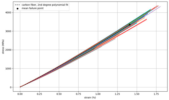
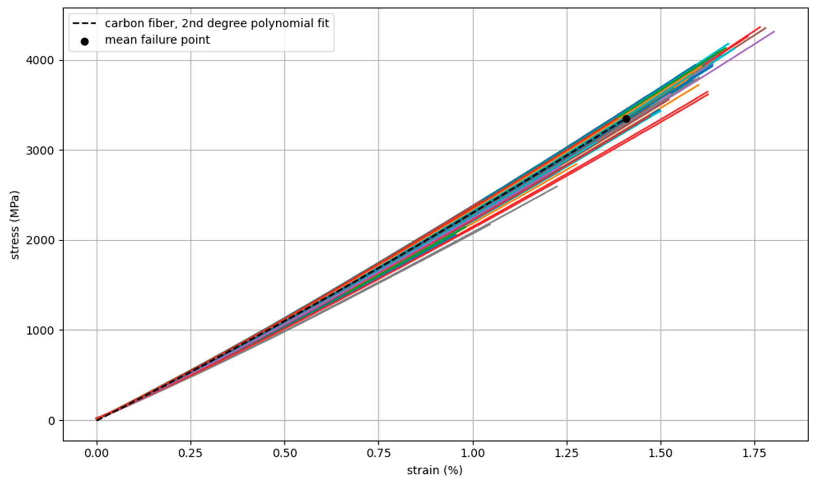
The measured tensile stress–strain curves of the 154 single fibers tested for a gauge length of 50 mm can be seen on Figure 2. Through these curves, the tensile Young’s modulus was calculated, being equal to E = (213 ± 5) GPa. The second-order polynomial fitting of the curves is shown, and the mean failure point of the single carbon fibers is annotated, at a stress of 3349 MPa and a 1.41% strain. Section 3.1.2 describes the calculation process. The obtained tensile properties (strength, strain at failure, and Young’s modulus) are within the range reported in the literature [8,23,26,27,28].

Figure 2. Tensile stress–strain curves of the 154 single carbon fibers tested (50 mm gauge length). Their second-order polynomial fitting line is also shown, and the mean failure point is annotated.

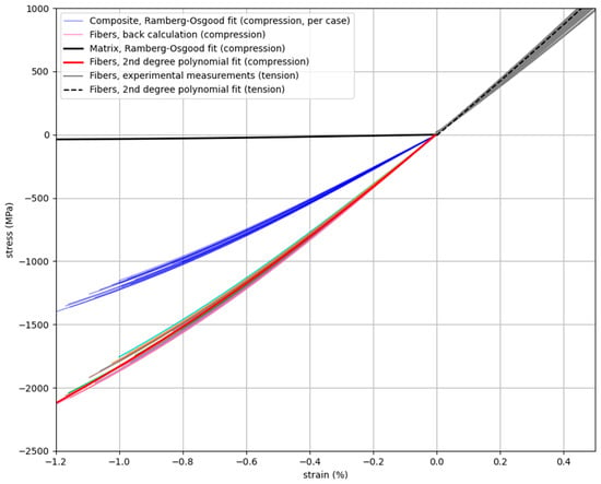
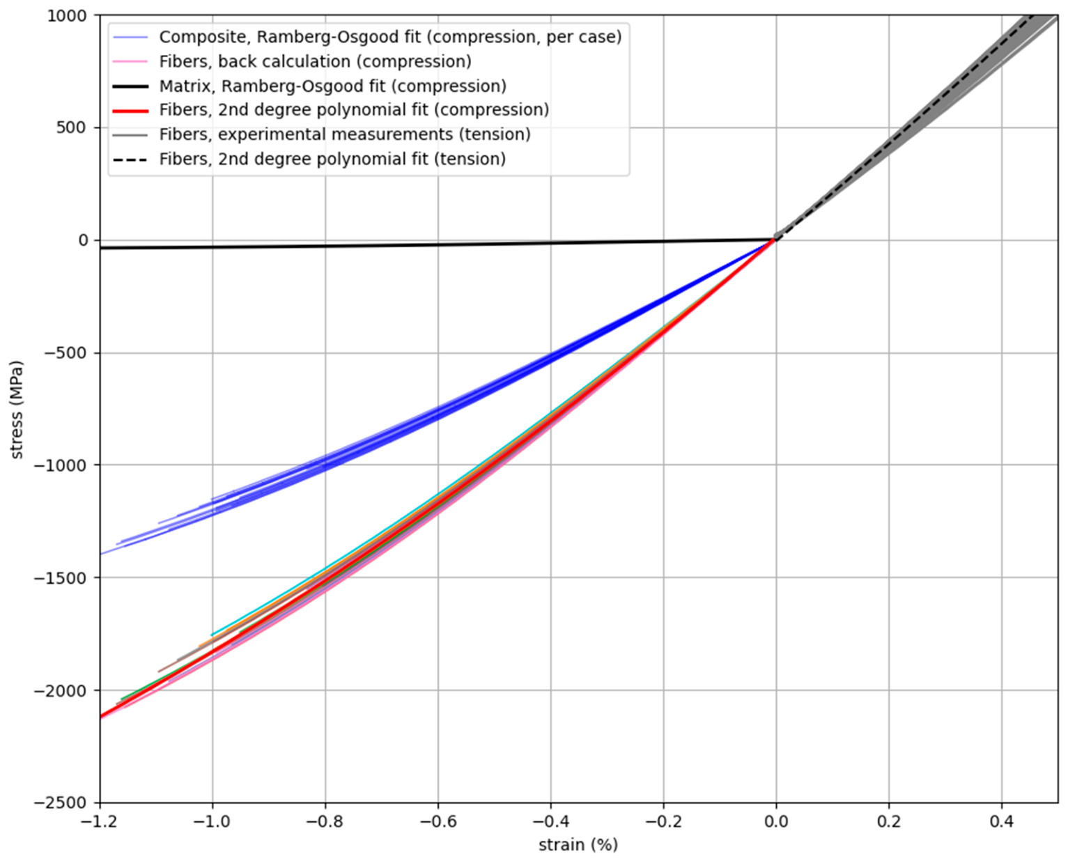
In total, 17 composite samples were subjected to compressive testing. Their stress–strain curves were used for the back calculation of the fibers’ compressive stress–strain graph, shown in Figure 3. For the back calculation, the compressive data for the matrix, namely the fit to the Ramberg–Osgood material model, was also used. The back calculation is explained in detail in Section 3.1.3. The compressive Young’s modulus was E_C = 204.1 GPa. The Young’s moduli were calculated over a strain range of [0.05–0.25]%.

Figure 3. Compressive stress–strain back-calculated curves of the fiber material, along with their average curve. The Ramberg–Osgood fitting of the compressive matrix stress–strain curve, as well as those for all the examined 17 composite samples, are shown. The tensile stress–strain curves of the tested single fibers, along with their fits, are also included.

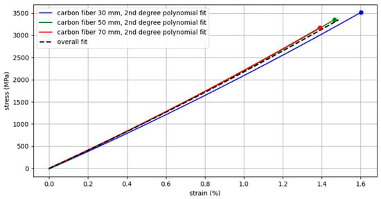
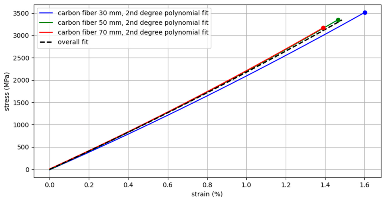
In addition to a gauge length of 50 mm, single-fiber testing was conducted at 30 mm and 70 mm, yielding a total of 255 single fibers. In Figure 4, a second-order polynomial fit of the stress–strain data for the three gauge lengths is shown. The machine’s compliance was considered, as described in Section 3.1.2. The mean failure points are annotated. For each gauge length (30 mm, 50 mm, and 70 mm, respectively), the mean failure was at σ = 3519 MPa, σ = 3350 MPa, and σ = 3175 MPa, with the corresponding values of the failure strain being ε = 1.48%, ε = 1.41%, and ε = 1.34%, in the same gauge length order as above. In addition, the overall second-degree polynomial fitting stress–strain curve is included.

Figure 4. Second-degree polynomial fitting stress–strain curves for all three gauge lengths examined (30 mm, 50 mm, and 70 mm). Their mean failure points are annotated. The overall fitting curve is also shown.

2.1.3. Fiber Modulus

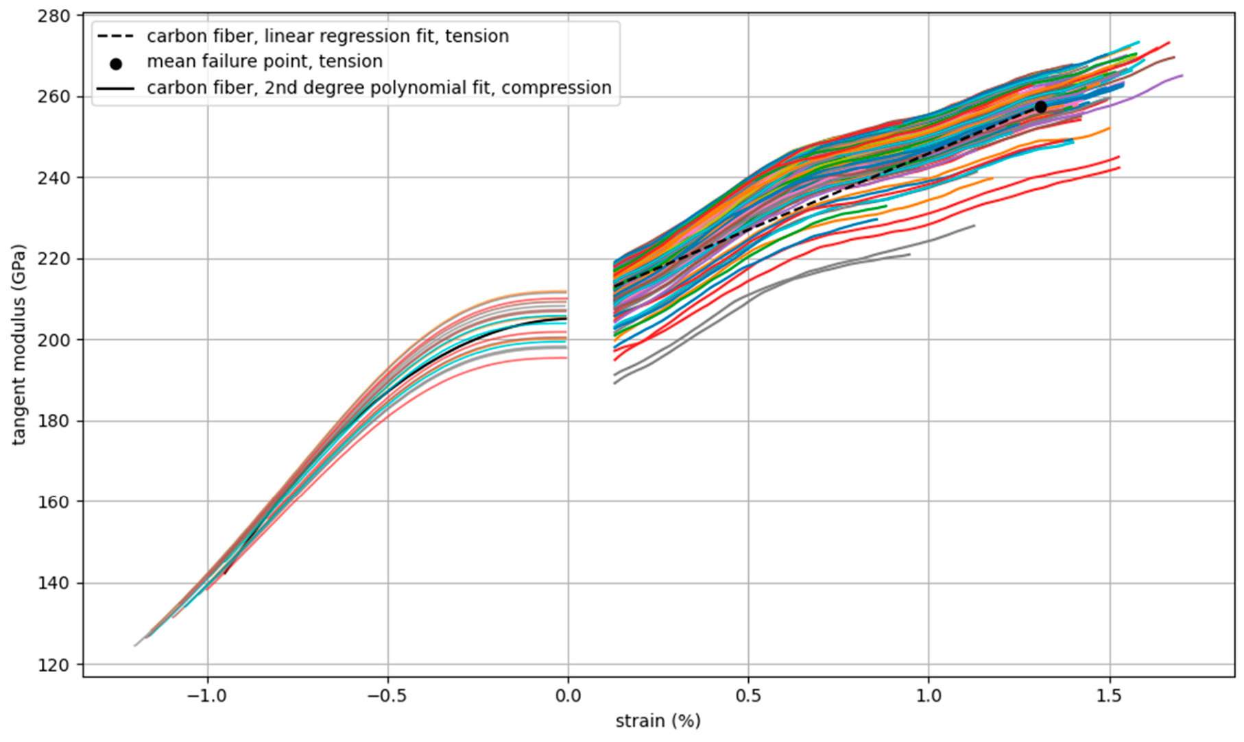
The tangent modulus, $E_t={\displaystyle \frac{d\sigma }{d\epsilon }}$, was calculated for both the tested single fibers under tension and the fibers back-calculated for compression (Figure 5). First, the tangent modulus-strain curves of the 50 mm gauge length fibers subjected to tensile testing were plotted. After applying linear regression to these curves, the equation describing the linear fitting was found to be the following:

$$E_{t, tension}=38.22{\displaystyle \frac{\mathrm{G}\mathrm{P}\mathrm{a}}{\%}}·\epsilon [\%]+207.32 \mathrm{G}\mathrm{P}\mathrm{a}$$

(1)

Figure 5. Tangent modulus—strain graph of the single fibers tested under tension (gauge length: 50 mm), as well as for the back-calculated compression ones. The fitting of each case is shown, while the corresponding mean failure point regarding tension is also annotated.

The mean failure point is indicated in Figure 5 at a strain of ε = 1.41% with a tangent modulus at the failure point of E_t,tension = 261.21 GPa. Considering Equation (1), the initial modulus is $E_{0,tension}=207.32 \mathrm{G}\mathrm{P}\mathrm{a}$, with a curvature coefficient $a=38.22{\displaystyle \frac{\mathrm{G}\mathrm{P}\mathrm{a}}{\%}}$. The same process was applied for the back-calculated compressive stress–strain. Here, the fit used for the compressive stress–strain curves was a second-degree polynomial:

$$E_t=\{\begin{array}{c}38.22{\displaystyle \frac{\mathrm{G}\mathrm{P}\mathrm{a}}{\%}}·\epsilon [\%]+207.32 \mathrm{G}\mathrm{P}\mathrm{a} \mathrm{f}\mathrm{o}\mathrm{r} \epsilon >0\\ -67.96{\displaystyle \frac{\mathrm{G}\mathrm{P}\mathrm{a}}{{\%}^2}}·{\epsilon }^2{\left[\%\right]}^2+2.75{\displaystyle \frac{\mathrm{G}\mathrm{P}\mathrm{a}}{\%}}·\epsilon [\%]+205.24 \mathrm{G}\mathrm{P}\mathrm{a} \mathrm{f}\mathrm{o}\mathrm{r} \epsilon <0 \end{array}$$

(2)

2.1.4. Fiber Failure Stress and Weibull Model Parameters Determination

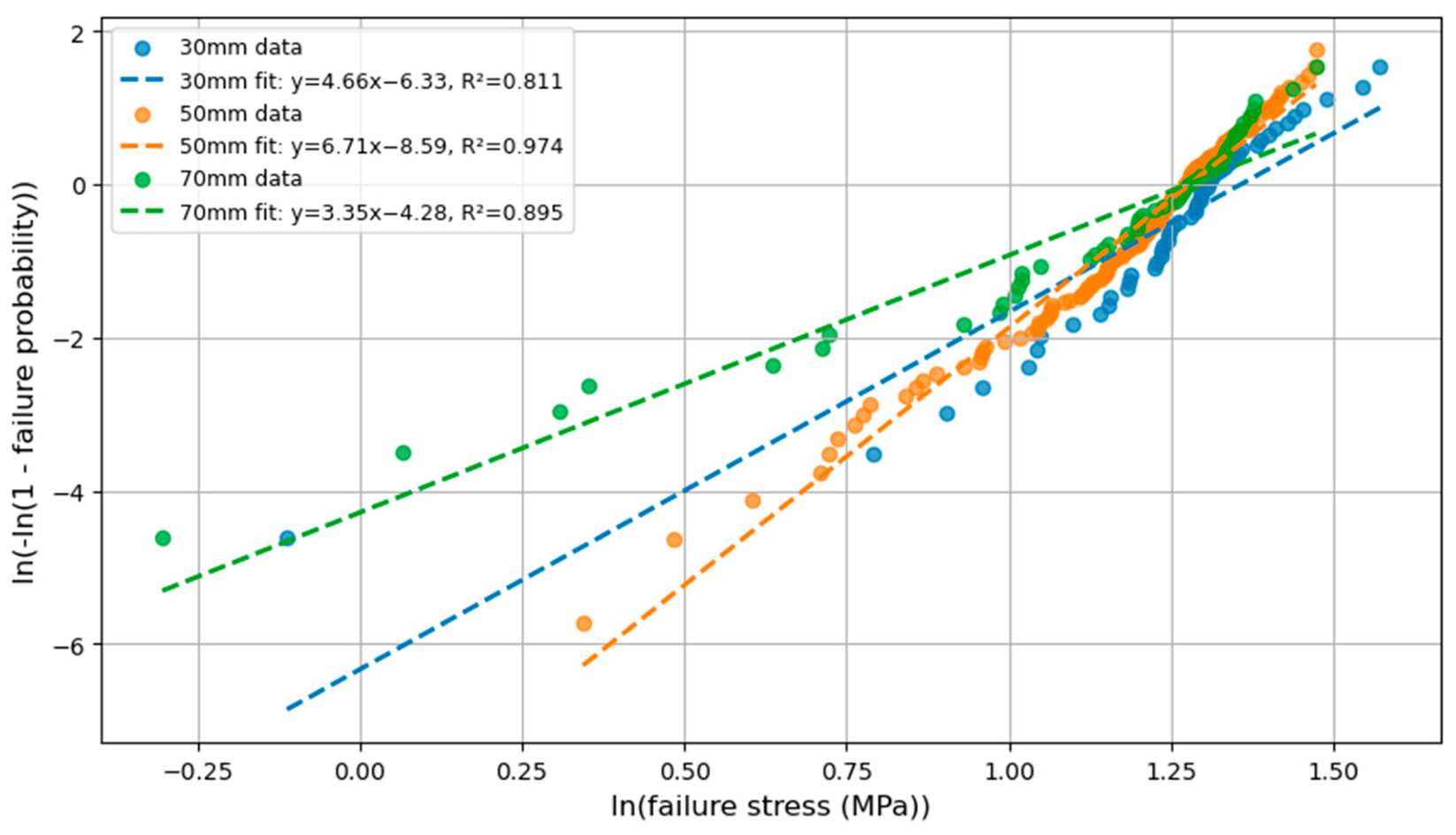
The Weibull model was applied to the measured single carbon fibers regarding the three-gauge lengths examined (30 mm, 50 mm, and 70 mm). In Figure 6, the Weibull plot of the measured failure stress is shown, along with the linear fits for each case obtained via maximum likelihood estimation. Table 1 shows the Weibull model parameters for each gauge length. These include the Weibull modulus m, the characteristic failure stress σ₀, the measured median failure stress $\tilde{\sigma }$, the measured mean failure stress $\overline{\sigma }$, and the stress-length factor ${\sigma }_0^{\overline{m}}·L_0$, which is a length-scale-independent value. The overall mean Weibull modulus, $\overline{m}$ = 5.90, while the overall mean stress-length factor ${\sigma }_0^{\overline{m}}·L_0$= (98.94 ± 20.19) ${\mathrm{G}\mathrm{P}\mathrm{a}}^{\overline{\mathrm{m}}}$m. Considering the value of $\overline{m}$, the aforementioned unit is, in this case, GPa^5.90m. Details on the implementation of the Weibull model are provided in Section 3.1.4.

Figure 6. The Weibull plots of the failure stress of the single carbon fibers tested, for each examined gauge length (30 mm, 50 mm, and 70 mm). The linear fit lines, along with their equations and the corresponding coefficients of determination, are included.

Table 1. The Weibull model parameters (Weibull modulus and characteristic failure stress), along with the median and mean failure stress, are shown for each gauge length of the single carbon fibers tested. The stress-length factor is also included. The mean values of the Weibull modulus and the stress-length factor are shown. Due to the non-linearity and the R²-value (R² = 0.895) of the 70 mm case, the mean Weibull modulus and stress-length factor regarding the 30 mm and 50 mm gauge lengths are also included.

Gauge Length L0 [mm]	Weibull Modulus m [-]	Characteristic Failure Stress σ0 [GPa]	Median Failure Stress $\tilde{\mathit{\sigma }}$ (Measured) [GPa]	Mean Failure Stress $\overline{\mathit{\sigma }}$ (Measured) [GPa]	Stress-Length Factor ${\mathit{\sigma }}_0^{\overline{\mathit{m}}}·{\mathit{L}}_0$ $[{\mathbf{G}\mathbf{P}\mathbf{a}}^{\overline{\mathbf{m}}}$m]
30	7.39	3.78	3.62	3.52	76.21
50	6.71	3.60	3.44	3.35	95.33
70	3.60	3.56	3.37	3.18	125.27
Mean	5.90				98.94 ± 20.19
Mean (30 and 50 mm)	7.05				85.77 ± 9.56

2.1.5. Scaling of the Fiber Failure Stress with the Gauge Length

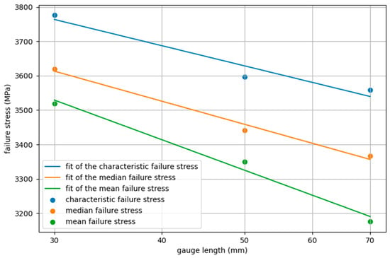
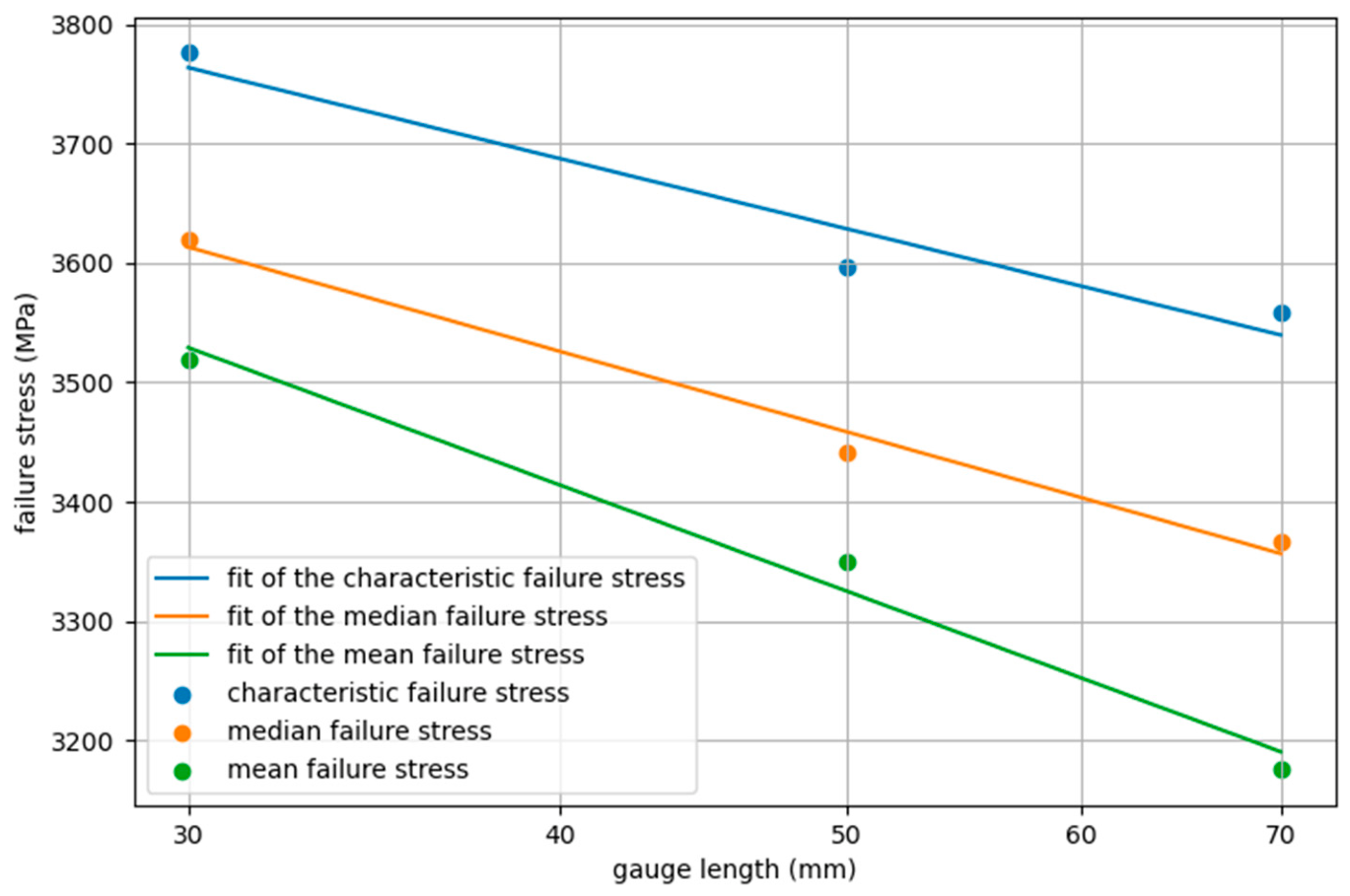
Figure 7 shows the scaling of the characteristic σ₀, median $\tilde{\sigma }$ and mean $\overline{\sigma }$ failure stresses for all three gauge lengths considered. Following a similar analysis to the one done by Kumar et al. [8], the Weibull modulus m for the linear fitting curves of the aforementioned failure stresses was found to be m₀ = 14.13 for the characteristic failure stress σ₀, m_median = 11.84 for the median failure stress $\tilde{\sigma }$ and m_mean = 8.34 for the mean failure stress $\overline{\sigma }$.

Figure 7. Logarithmic graph of the characteristic, median, and mean failure stress of the single carbon fibers for each gauge length, including the related linear fitting curves.

2.2. Matrix

2.2.1. Matrix Tensile Stress–Strain Curves

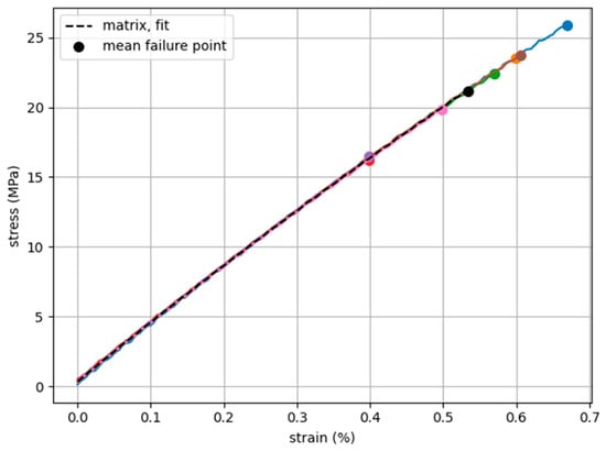
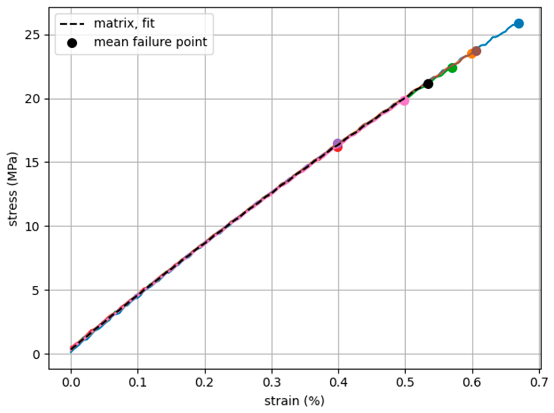
Figure 8 shows the stress–strain curves for the matrix subjected to tensile testing (as described in Section 3.2.1). Seven samples were tested. The tensile strength ranged from σ_max = 16.22 MPa to σ_max = 25.85 MPa, and the strain from ε = 0.40% to ε = 0.67%. The mean strength, annotated as the mean failure point, was $\overline{\sigma }$_max = 21.15 MPa, at a mean failure strain of ε = 0.53%. Considering this, the average Young’s modulus was E_m = 4.08 GPa, with its values ranging from E_m = 4.04 GPa to E_m = 4.12 GPa. The obtained Young’s modulus is within the range reported for vinyl ester systems in the literature [29,30].

Figure 8. Tensile stress–strain curves for the matrix material, with the failure point annotated. The fitting curve, along with the mean failure point, are also shown.

2.2.2. Matrix Shear Stress–Strain Curves

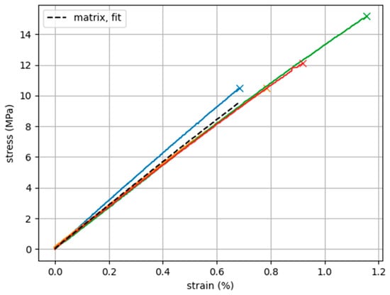
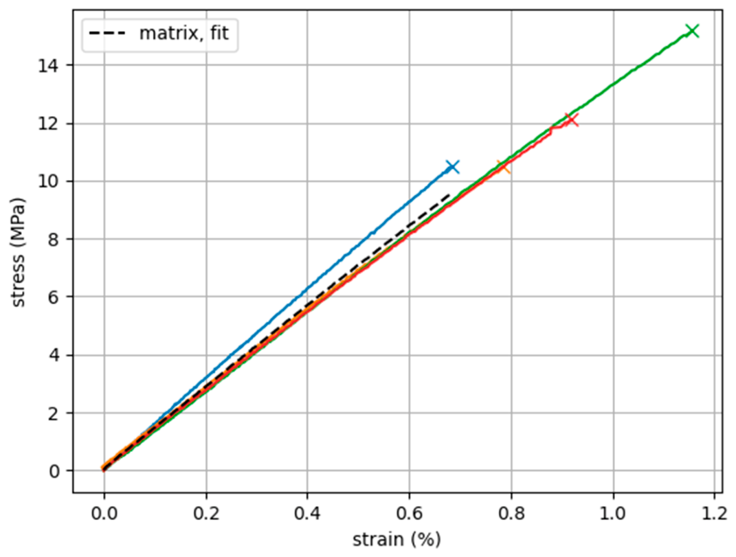
In Figure 9, the shear stress–strain curves for the vinyl ester matrix material are shown. The details of the mechanical testing are included in Section 3.2.2. Four samples were subjected to Iosipescu shear testing [31]. The maximum shear stress ranged from $\tau$_max = 10.48 MPa to $\tau$_max = 15.17 MPa, and the maximum shear strain from γ = 0.69% to γ = 1.16%. The fitting curve of the results is also included. The shear modulus was G = (1.41 ± 0.1) GPa. These values are consistent with the vinyl ester shear properties reported in [29,30], indicating that the obtained results are within the expected range.

Figure 9. Shear stress–strain curves for the matrix material, with the failure point annotated. The fitting curve is also shown.

2.2.3. Matrix Von Mises Stress–Strain Curves

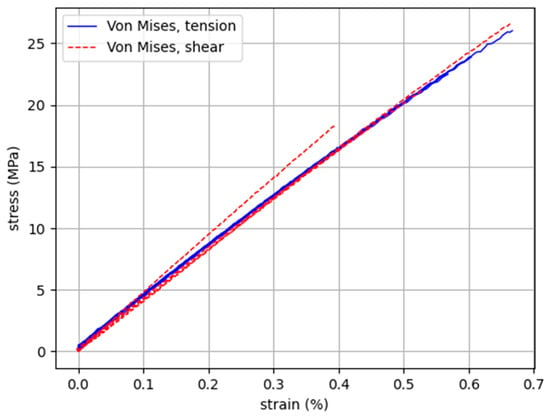
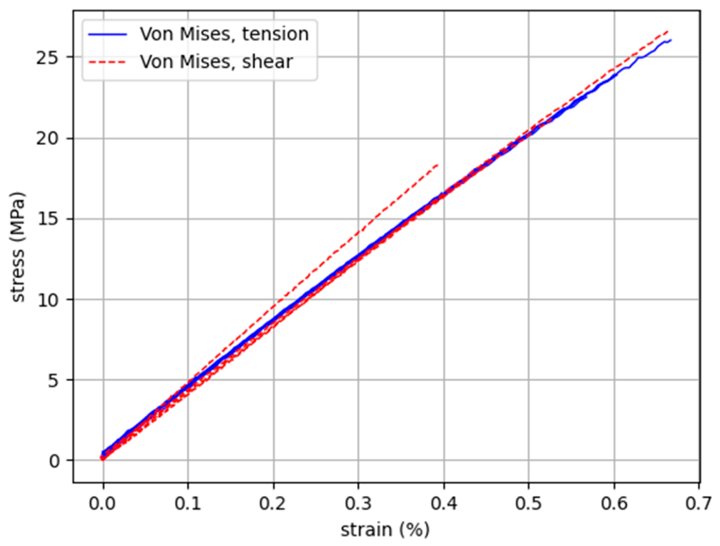
The von Mises stress–strain curves were calculated using the measurements acquired from both the tensile and the shear tests (Figure 10). The average maximum value of the effective stress is σ_eq,m = 21.2 MPa, while the highest value is σ_eq,m = 26.6 MPa.

Figure 10. Von Mises stress–strain curves for the matrix material under tension and shear.

2.2.4. Ramberg–Osgood Material Model

The Ramberg–Osgood material model was used to describe the nonlinear matrix behavior in the numerical model presented in [13]. For this reason, the experimental stress–strain data, acquired through tensile testing, should fit into the model, whose equation is

$${\epsilon }_{eq,m}={\displaystyle \frac{{\sigma }_{eq,m}}{E_m}}+{\displaystyle \frac{3}{7}}{{\displaystyle \frac{{\sigma }_{0,m}}{E_m}}\left({\displaystyle \frac{{\sigma }_{eq,m}}{{\sigma }_{0,m}}}\right)}^{n_m}$$

(3)

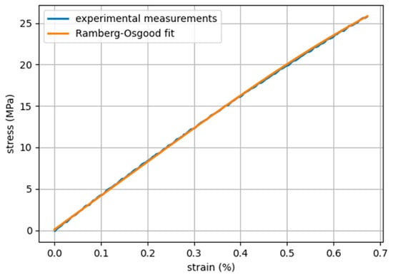
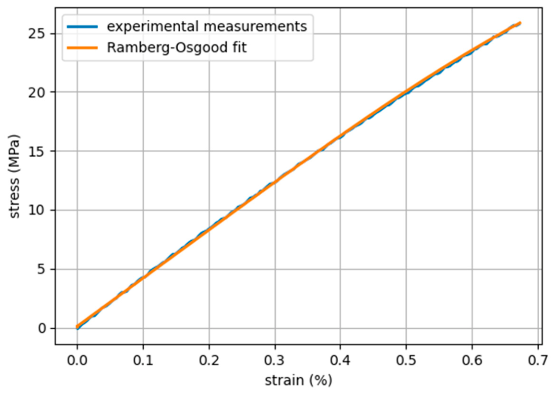
where ${\epsilon }_{eq,m}$ is the equivalent von Mises strain, ${\sigma }_{eq,m}$ is the equivalent von Mises stress, E_m, is the matrix’s Young’s modulus, and ${\sigma }_{0,m}=40.056$ MPa and $n_m=5.213$ are the two fitting parameters of the Ramberg–Osgood material model. The calculation steps are described in detail in Section 3.2.3. Figure 11 shows the Ramberg–Osgood fit along with the experimental data, showing a very good agreement over the examined strain range.

Figure 11. The experimental measurements of the stress and strain of the matrix, under tensile testing, along with the Ramberg–Osgood fit of them.

2.3. Composite

2.3.1. X-Ray CT-Scanned Composite Data

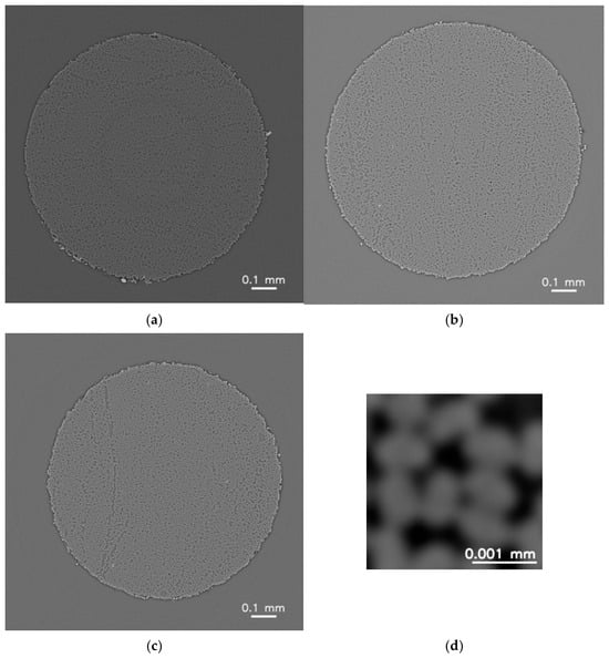
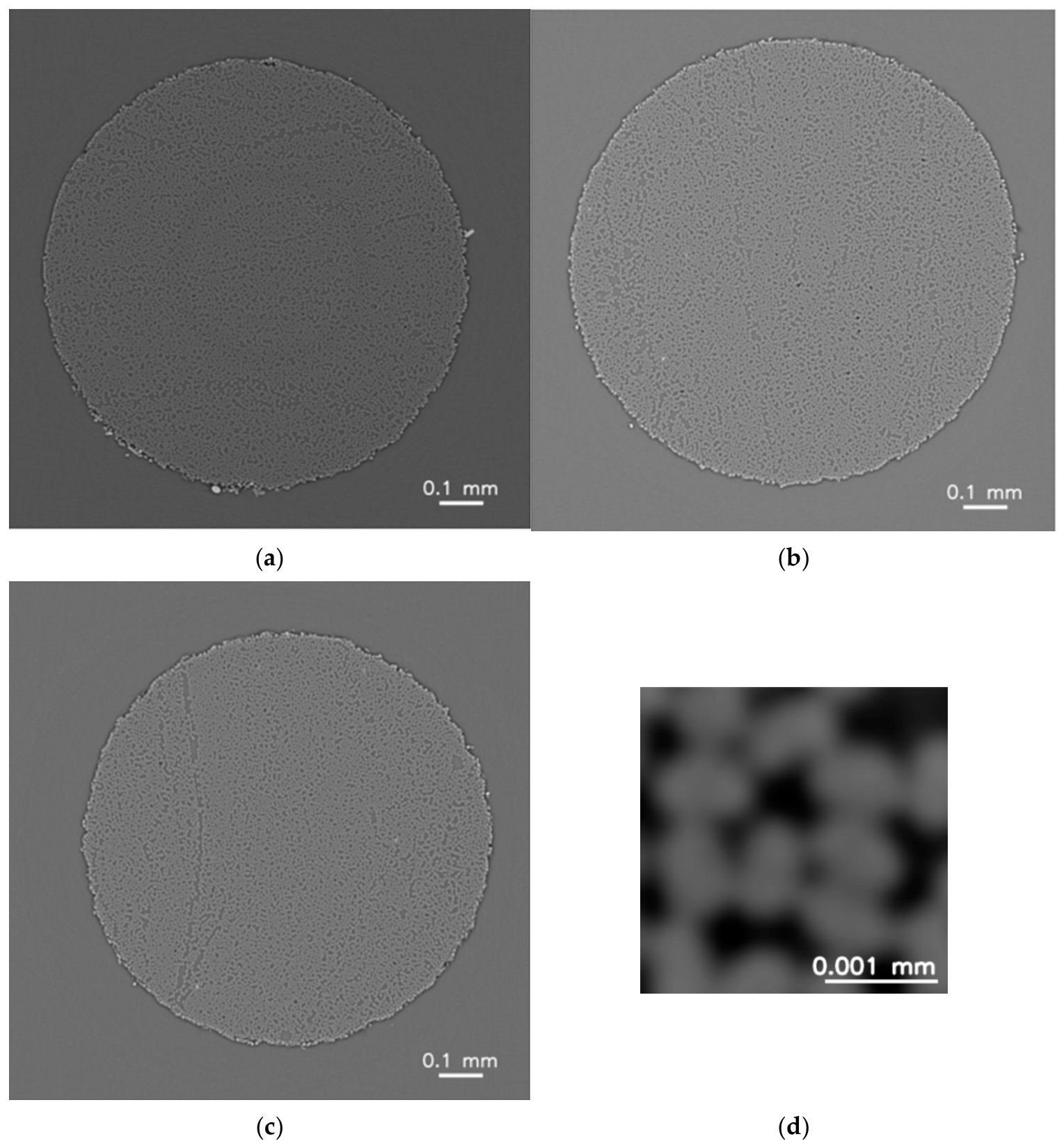
Three cylindrical samples were cut from the unidirectional carbon fiber pultruded profiles. The samples had a diameter of 1 mm. These samples were subjected to X-ray CT scanning at the DanMAX beamline of the MAX IV synchrotron facility. The scanning parameters are shown in Table 2. The acquired datasets consisted of 2178 projections per scan, which were used for tomographic reconstruction. The three reconstructed datasets were stored in HDF5 (Hierarchical Data Format version 5) format. For easier handling and visualization, the reconstructed image files were extracted as 2204 separate TIFF (Tagged Image File Format) slices per dataset (Figure 12). The total size of each dataset was 39 GB. The data of the X-ray CT samples can be found on [16,17,18].

Table 2. The X-ray scanning parameters.

Parallel Beam Energy [keV]	Projections per Dataset	Propagation Distance [mm]
35	2178	90
Projection field [mm3]	Exposure time for each projection [sec]	Voxel size [μm]
1.2 × 1.2 × 1.2	0.06	0.55

Figure 12. (a–c) Reconstructed images of the cross-section of samples A, B, and C, respectively; (d) zoomed detailed area of sample (B). The fiber kidney-shaped cross-section is visible.

2.3.2. SEM Image of the Material

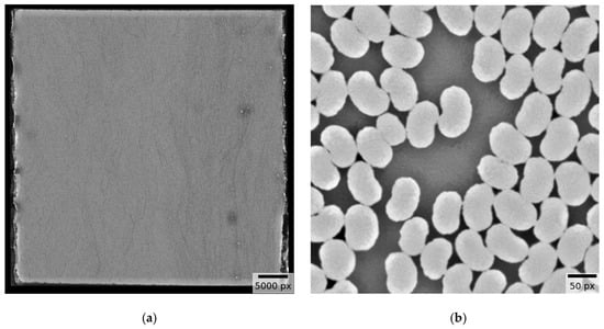
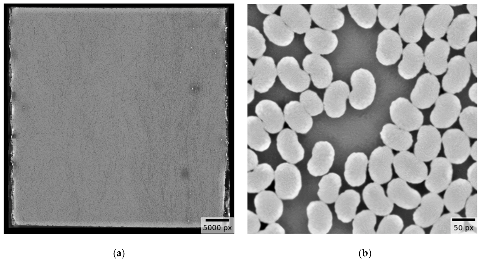
A sample of the same composite material was analyzed by SEM to determine the fiber volume fraction (as described in Section 3.3.4). In Figure 13, the scanned image can be seen along with a cropped detail, in which the fibers and the matrix are distinguished. The characteristic shape of the cross-section of the carbon fibers, resembling the shape of a kidney, can also be noted. The SEM parameters are presented in Table 3.

Figure 13. (a) The SEM image of the sample; (b) a zoomed part of the image, in which the carbon fiber material can easily be distinguished from the matrix.

Table 3. The SEM parameters, used for the acquisition of the SEM image.

Pixel Size Scan [nm]	Physical Size [mm2]	Magnification	Detector
97.66	5.12 × 5.16	3400	BSD Full
Scan size [pixels]	Exposure time [s/scan]	High voltage [kV]	Overlap [pixels]
52,439 × 52,844	<1	15	102

2.3.3. Composite Fiber Density Data

The burn-off method is widely used to determine the fiber density of the composite material [32,33,34]. In this work, coupons were cut to determine the fiber and porosity content of each pultruded profile from which the samples were subjected to X-ray scanning. The base material of the profiles was the same, but the pultrusion manufacturing parameters were varied. The density of the matrix was ρ_m = 1.16 g/cm³, and the density of the fibers was ρ_f = 1.81 g/cm³. Table 4 shows the coupons, named A_vfx, B_vfx, and C_vfx, with A, B, and C corresponding to the respective X-ray scanned samples, and x denoting the coupon number. For scanned samples A and C, the number of coupons used for determining the fiber content was five, and for sample B was three. A description of the method is provided in Section 3.3.3. The measured fiber volume fraction and composite density are consistent with the values of pultruded unidirectional carbon fiber composites reported in the literature [35,36,37].

Table 4. The fiber, matrix, and porosity content of the composite material; the weight content of the fibers and the matrix; the composite density; and the weight of the fibers and the sealing, all for different tested coupons. The coupons correspond to the three datasets of the X-ray scanned samples. The fiber density was ${\rho }_f=1.81 \mathrm{g}/{\mathrm{c}\mathrm{m}}^3$ and matrix density was ${\rho }_m=1.16 \mathrm{g}/{\mathrm{c}\mathrm{m}}^3$.

Sample	Sample Weight [g]	Fibers Weight [g]	Sealing Weight [g]	Composite Density [g/cm3]	Fibers Weight Content [%]	Matrix Weight Content [%]	Fibers Volume Content [%]	Matrix Volume Content [%]	Porosity Volume Content [%]
A_vf1	1.628	1.218	0.0071	1.572	74.8	25.2	65.0	34.2	0.9
A_vf2	1.626	1.215	0.0064	1.572	74.7	25.3	64.9	34.3	0.9
A_vf3	1.629	1.218	0.0076	1.571	74.8	25.2	64.9	34.2	0.9
A_vf4	1.562	1.169	0.0059	1.573	74.8	25.2	65.0	34.1	0.8
A_vf5	1.615	1.197	0.0059	1.570	74.1	25.9	64.3	35.0	0.7
Mean				1.572	74.6	25.4	64.8	34.4	0.8
Standard Deviation				0.001	0.3	0.3	0.3	0.4	0.1
B_vf1	1.590	1.174	0.0062	1.567	73.9	26.1	64.0	35.3	0.7
B_vf2	1.607	1.190	0.0067	1.569	74.0	26.0	64.2	35.1	0.7
B_vf3	1.623	1.203	0.0069	1.572	74.1	25.9	64.3	35.1	0.6
Mean				1.600	74.0	26.0	64.2	35.2	0.7
Standard Deviation				0.002	0.1	0.1	0.2	0.1	0.1
C_vf1	1.621	1.210	0.0077	1.584	74.7	25.3	65.3	34.6	0.1
C_vf2	1.633	1.240	0.0073	1.591	75.9	24.1	66.8	33.0	0.3
C_vf3	1.626	1.236	0.0083	1.589	76.0	24.0	66.7	32.9	0.4
C_vf4	1.613	1.203	0.0072	1.583	74.6	25.4	65.3	34.7	0.1
C_vf5	1.637	1.243	0.0069	1.591	75.9	24.1	66.8	33.0	0.2
Mean				1.588	75.4	24.6	66.2	33.6	0.2
Standard Deviation				0.004	0.7	0.7	0.8	0.9	0.1

2.3.4. Composite Compression Stress–Strain Curves

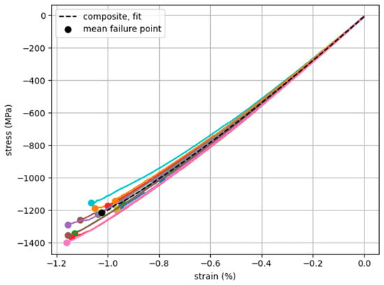
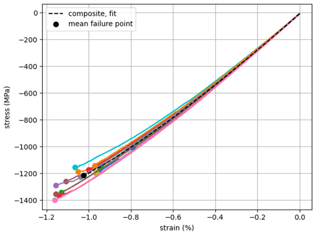
Compression testing was carried out on 17 specimens cut from the three pultruded profiles used to acquire the scanned samples. The compressive strength ranged from σ_max = 1010 MPa to σ_max = 1399 MPa, while the compressive strain ranged from ε = 0.80% to ε = 1.17%. The average compressive strength was $\overline{\sigma }$_max = 1214 MPa, and the average compressive strain $\overline{\epsilon }$ = 1.02%. The average Young’s modulus was E = 134 GPa, ranging from E = 128 GPa to E = 139 GPa. The stress–strain curves from the compression tests are shown in Figure 14, while details of the test procedure are provided in Section 3.3.2. Considering [37,38,39], the acquired properties are within the expected range for pultruded carbon composites under compression.

Figure 14. Stress–strain curves of composite samples, under compressive loading. The failure points are marked. The fit line is included, with the mean failure point marked.

Using the average measured fiber volume fraction of the three burn-off coupon groups, V_f = 65.2%, the average measured matrix volume fraction, V_m = 34.8%, the fiber modulus in compression, Ef,_C = 204.1 GPa, and the matrix modulus, E_m = 4.08 GPa, the rule of mixtures gives an expected composite modulus of E = 134.5 GPa, calculated as

$$E=V_f·E_{f,C}+V_m·E_m$$

(4)

The predicted value is in very good agreement with the experimental result.

2.3.5. Histograms of the Fiber Orientation Distribution

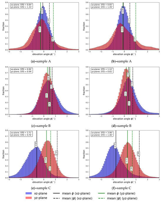
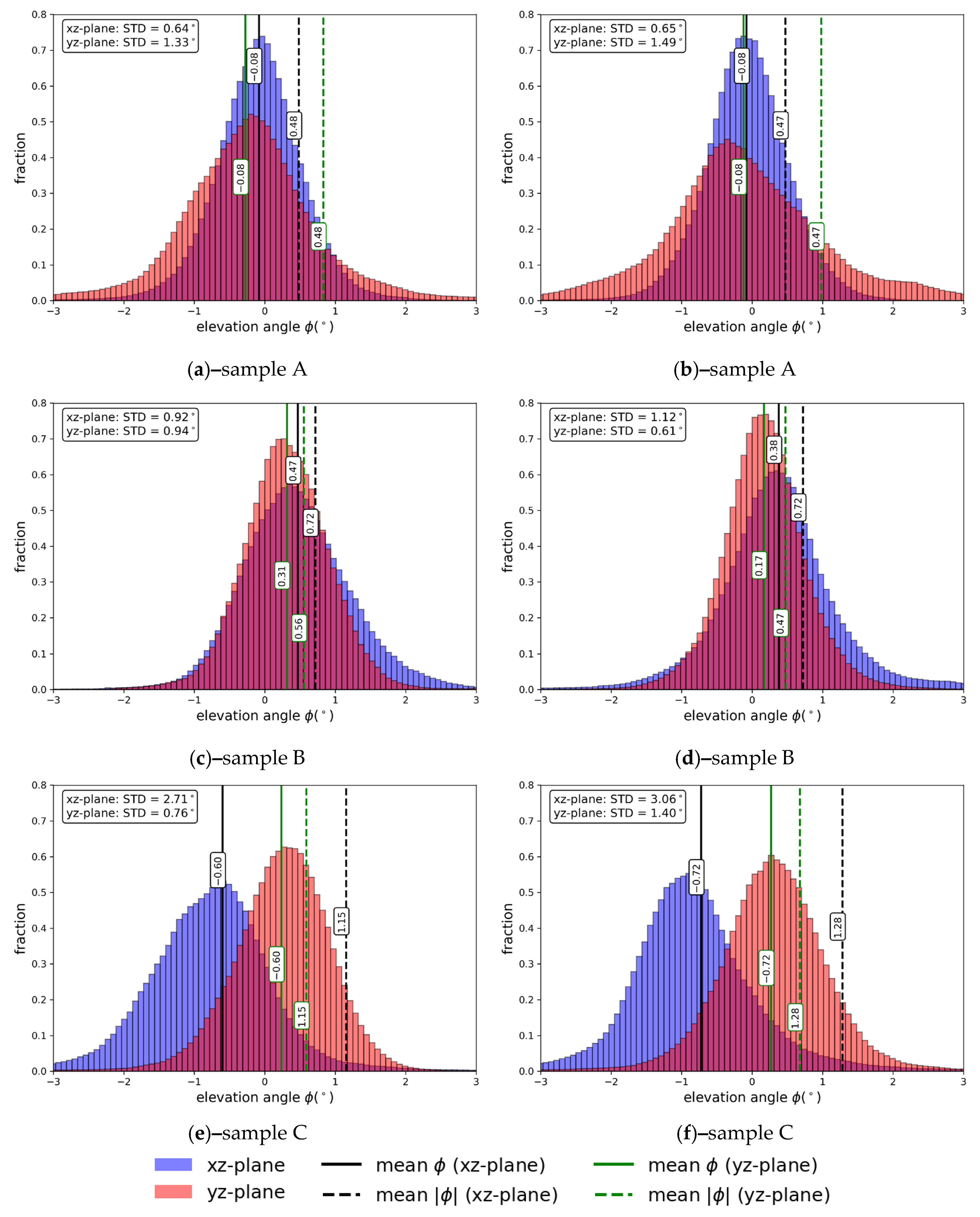
Figure 15 illustrates the histograms of the fiber orientation distribution, determined using the structure tensor analysis (Section 3.3.5) for two slices per plane in each sample. Each histogram corresponds to the fiber orientation of two slices (from a single sample), extracted from the corresponding xz- and yz-planes, respectively. The average values of the mean elevation angle, $\overline{\phi }$, and the mean absolute elevation angle, $\overline{\left|\phi \right|}$, for each sample and plane are presented in Table 5. The mean elevation angle shows any potential directional bias. In contrast, the mean absolute elevation angle serves as an indicator of both the average orientation and its scatter, described by a single value. The histogram of elevation angles remains the primary descriptor of the orientation distribution, as it captures the variability across the analyzed volume. Similar orientation distribution patterns for unidirectional carbon fiber composites can be found in [11,38].

Figure 15. Histograms of the fiber orientation distribution for two slices per plane per dataset, including the mean elevation angle, $\overline{\phi }$, and the mean absolute elevation angle, $\overline{\left|\phi \right|}$. The standard deviation (STD) of the distributions is also reported. (a,b) Histograms of the first sample; (c,d) histograms of the second sample; (e,f) histograms of the third sample.

Table 5. The average values of the mean elevation angle and the mean absolute elevation angle per dataset.

Sample	Plane	Mean Elevation Angle $\overline{\mathit{\phi }}$ [°]	Mean Absolute Elevation Angle $\overline{\left|\mathit{\phi }\right|}$ [°]
A	xz	−0.01 ± 0.56	0.86 ± 0.06
	yz	−0.11 ± 0.08	0.56 ± 0.08
B	xz	0.40 ± 0.05	0.76 ± 0.03
	yz	0.23 ± 0.07	0.54 ± 0.04
C	xz	−0.63 ± 0.10	1.24 ± 0.05
	yz	0.19 ± 0.15	0.63 ± 0.07

3. Methods

3.1. Fibers

3.1.1. Fiber Linear Density and Diameter Calculation

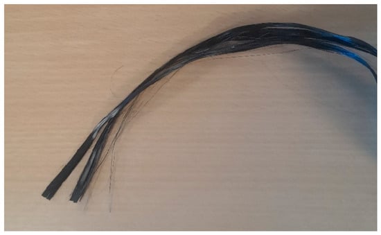
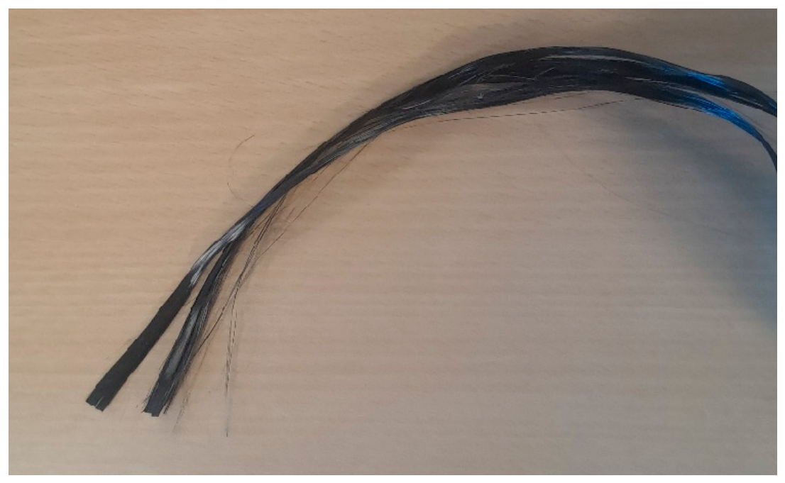
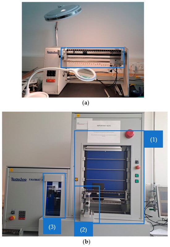
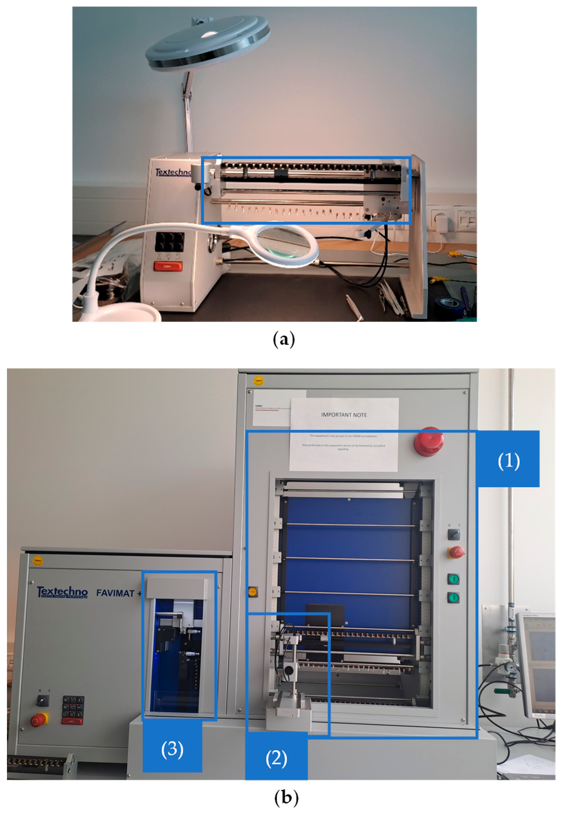
The first step in determining the linear density of the carbon fibers was the separation of the single fibers from the carbon fiber tow (Figure 16). Given the desired gauge length of 50 mm, a slightly larger section of the tow was cut. From this, the single fibers were manually separated with a paintbrush to minimize fiber breakage. After a single fiber was separated, a 0.1 g weight was clamped to it. The single fibers were then inserted into a magazine (Figure 17a), which could hold up to 25 fibers, and were hung vertically in place by their clamped weights. The magazine was transferred to the magazine region of the automatic single fiber test machine FAVIMAT+, which is used for single fiber testing (Figure 17(b1)).

Figure 16. Carbon fiber tow, from which single fibers were separated and used for single fiber testing. Each tow contains approximately 50,000 single fibers.

Figure 17. (a) The magazine. The clamps that keep the single fibers straight are shown. (b) The automatic single fiber test machine FAVIMAT+: (1) the magazine area; (2) the robot; (3) the testing region.

From there, a robot (Figure 17(b2)) grabbed every single fiber and transferred it to the testing region (Figure 17(b3)), where it was gripped between two clamps. The linear density, μ, was determined from the resonance frequency, f, measured using a vibroscope integrated in the machine. A pre-tension of F_v = 2 cN/tex was used, and the iterative analysis developed by Madsen et al. [40,41] was subsequently used to precisely determine the linear density, μ. In more detail, the resonance frequency f is found as follows:

$$f={\displaystyle \frac{1}{2·L}}\sqrt{{\displaystyle \frac{F_v}{\mu }}}·\sqrt{1+{\displaystyle \frac{{\pi }^3·E·r_f^4}{4·L^2·F_v}}}$$

(5)

where L is the gauge length, E the true fiber modulus, and r_f the fiber radius. However, since

$$E·r_f^4\ll L^2·F_v$$

(6)

the last term of Equation (5) is negligible, and thus it can be simplified to

$$f={\displaystyle \frac{1}{2·L}}\sqrt{{\displaystyle \frac{F_v}{\mu }}}$$

(7)

Therefore, the linear density, μ, can be determined as

$$\mu ={\displaystyle \frac{F_v}{4·f^2·L^2}}$$

(8)

Using the material density of the carbon fiber of ρ_f = 1.81 g/cm³, the cross-sectional area of the fibers, A₀, can be calculated as

$$A_0={\displaystyle \frac{\mu }{{\rho }_f}}$$

(9)

It can be noted from the simplification of Equation (5) to Equation (7) to Equation (6), that the shape of the cross-section of the fiber does not affect the calculation of the cross-sectional area. The measurements were taken at a room temperature of 22.0 ± 0.4 °C and a humidity of 38%.

3.1.2. Fiber Tensile Testing

Immediately after the calculation of its diameter, each fiber was subjected to tensile testing in FAVIMAT+’s testing region (Figure 17(b3)). The pretension was set to approximately 0 N, and the test speed was 1 mm/min. By the time the fiber broke, ending its tensile test, the robot had already picked up the next fiber. During the seconds between unclamping and dropping the tested fiber and the robot’s placement of the next fiber, the clamps were manually cleaned with a brush. The test conditions were the same as those for the fiber density calculation, namely, the temperature was 22.0 ± 0.4 °C and the humidity was 38%.

The stress, σ, was calculated as

$$\sigma ={\displaystyle \frac{F}{A_0}}$$

(10)

where F is the measured force.

The strain ε could not be derived directly from the measured displacements due to the small displacements of the machine components. The main influence comes from local deformation of the rubber grips. Therefore, the machine compliance had to be defined to correct the displacement measurement of each fiber tensile test. To determine the machine compliance, C, the following equation was used:

$${\displaystyle \frac{1}{E^{*}}}=C·{\displaystyle \frac{A_0}{L_0}}+{\displaystyle \frac{1}{E}}$$

(11)

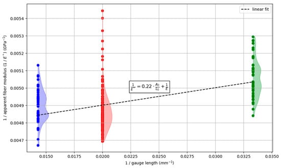
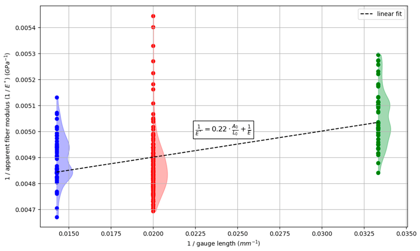
where E* is the apparent fiber modulus, L₀ the gauge length, and E the true fiber modulus. In addition to the 50 mm gauge length, two test series were performed with different gauge lengths (30 mm and 70 mm). Figure 18 shows the reciprocal of the apparent fiber modulus (1/E*) compared to the reciprocal of each fiber gauge length examined. To determine the essential correction of the machine compliance, the method described in [8] was followed. The equation of the data’s linear fit was calculated, with the slope describing the compliance C multiplied by the fiber’s cross-sectional area. It was found that C = 0.22 mm/N. The machine compliance was used for the correction of the measured displacement, $\Delta L$, as follows:

$${\Delta L}_{corr}=\Delta L-F·C$$

(12)

Figure 18. The reciprocal of the apparent fiber modulus (1/E*) compared to the reciprocal of each fiber gauge length examined. The linear fit and the equation used to calculate it are shown, where A₀ is the fiber cross-sectional area, L₀ is the gauge length, and E is the true fiber modulus. The distribution of the values of the reciprocal of the apparent fiber modulus for each gauge length is also included in the Figure.

Subsequently, the corrected strain ε is

$$\epsilon ={\displaystyle \frac{{\Delta L}_{corr}}{L_0}}$$

(13)

3.1.3. Fiber Compressive Stress–Strain Curves Calculation

To determine the fibers’ behavior under compressive loading, the matrix response was first described by fitting the Ramberg–Osgood material model, assuming similar behavior under pure tension and compression. This is a common approximation for vinyl ester matrices and is considered acceptable for the present analysis. The same material model was fitted to the stress–strain curves of each one of the 17 composite samples tested in compression. The Ramberg–Osgood material model fit, along with the composite’s compression tests, is described in the following sections. Based on these fits and the measured composite sample volume fractions, the fiber compressive stress–strain response was back-calculated using the rule of mixtures. This approach enables the estimation of fiber compressive behavior from experimentally measured composite response and constituent properties, as direct fiber compression measurements are not feasible. In addition, a second-degree polynomial was fitted to the fiber compressive stress–strain curves using least squares regression.

3.1.4. Fiber Failure Stress and Weibull Parameters Determination Analysis

The Weibull model was applied to statistically analyze the probability of failure of the examined carbon fiber material [42]. A two-parameter Weibull model [23,26], following the procedure described by Kumar et al. [8], is used to extract statistical strength parameters from the experimental dataset. For each gauge length, the failure stresses were ranked, converted into failure probabilities, and fitted to the Weibull distribution to determine the Weibull modulus and characteristic strength. The reader is referred to that work for a detailed description of the method. Below are the basic concepts for the two Weibull model parameters used.

The failure probability, $P_F$, at a given stress, $\sigma$, and a given length, L, is calculated as

$$P_F\left(\sigma ,L\right)=1-\exp \left(-{\displaystyle \frac{L}{L_0}}{\left({\displaystyle \frac{\sigma }{{\sigma }_0}}\right)}^m\right)$$

(14)

where L₀ is a reference length and ${\sigma }_0$ the characteristic failure stress at a failure probability P_F(σ₀, L₀) = 1 − exp(−1) = 0.6321, at the reference length. By rearranging the above equation, applying twice the logarithmic function, setting the reference length equal to the fiber material gauge length (L = L₀), and normalizing the given and the characteristic stress, it becomes the following:

$$\ln \left(-\ln \left(1-P_F\left(\sigma ,L\right)\right)\right) =m\ln \left({\displaystyle \frac{\sigma }{1 \mathrm{G}\mathrm{P}\mathrm{a}}}\right)-m\ln \left({\displaystyle \frac{{\sigma }_0}{1 \mathrm{G}\mathrm{P}\mathrm{a}}}\right)$$

(15)

where m is the Weibull modulus. It can be seen that Equation (15) is linear, of the form y = ax + b. The slope of the line, a, is the Weibull modulus, m, and the intercept of the line, b, is the term $-m\ln \left({\displaystyle \frac{{\sigma }_0}{1 \mathrm{G}\mathrm{P}\mathrm{a}}}\right)$.

The following steps were applied for each gauge length. First, the fiber sample size, N, was determined. For each one of them, the failure stress, $\sigma$, was found. The failure stress values, and thus the corresponding single fibers, were sorted from smallest to largest. A ranking was assigned to every single fiber, i; the fiber with the smallest failure stress value had i = 1, and the one with the largest failure stress had i = N. Then, for each fiber, the failure probability was calculated as

$$P_F\left({\sigma }_i,L\right)={\displaystyle \frac{i-0.5}{N}}$$

(16)

Considering the linear Equation (15), the x = $\ln \left({\displaystyle \frac{\sigma }{1 \mathrm{G}\mathrm{P}\mathrm{a}}}\right)$ and the y = $\ln \left(-\ln \left(1-P_F\left(\sigma ,L\right)\right)\right)$ can be found, resulting in N points of (x, y). After plotting all these points, and by following the maximum likelihood method [43], a fitted line was obtained. The slope of this line gives the Weibull modulus, m, and thus the characteristic strength ${\sigma }_0$ can be found through the intercept of the line, $-m\ln \left({\displaystyle \frac{{\sigma }_0}{1 \mathrm{G}\mathrm{P}\mathrm{a}}}\right)$.

3.2. Matrix

3.2.1. Matrix Tensile Testing

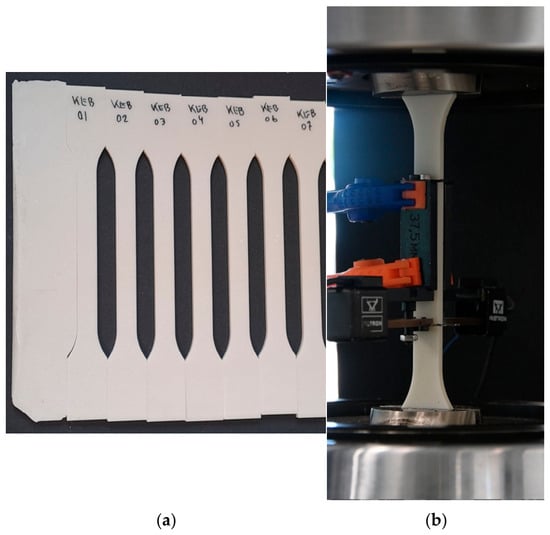
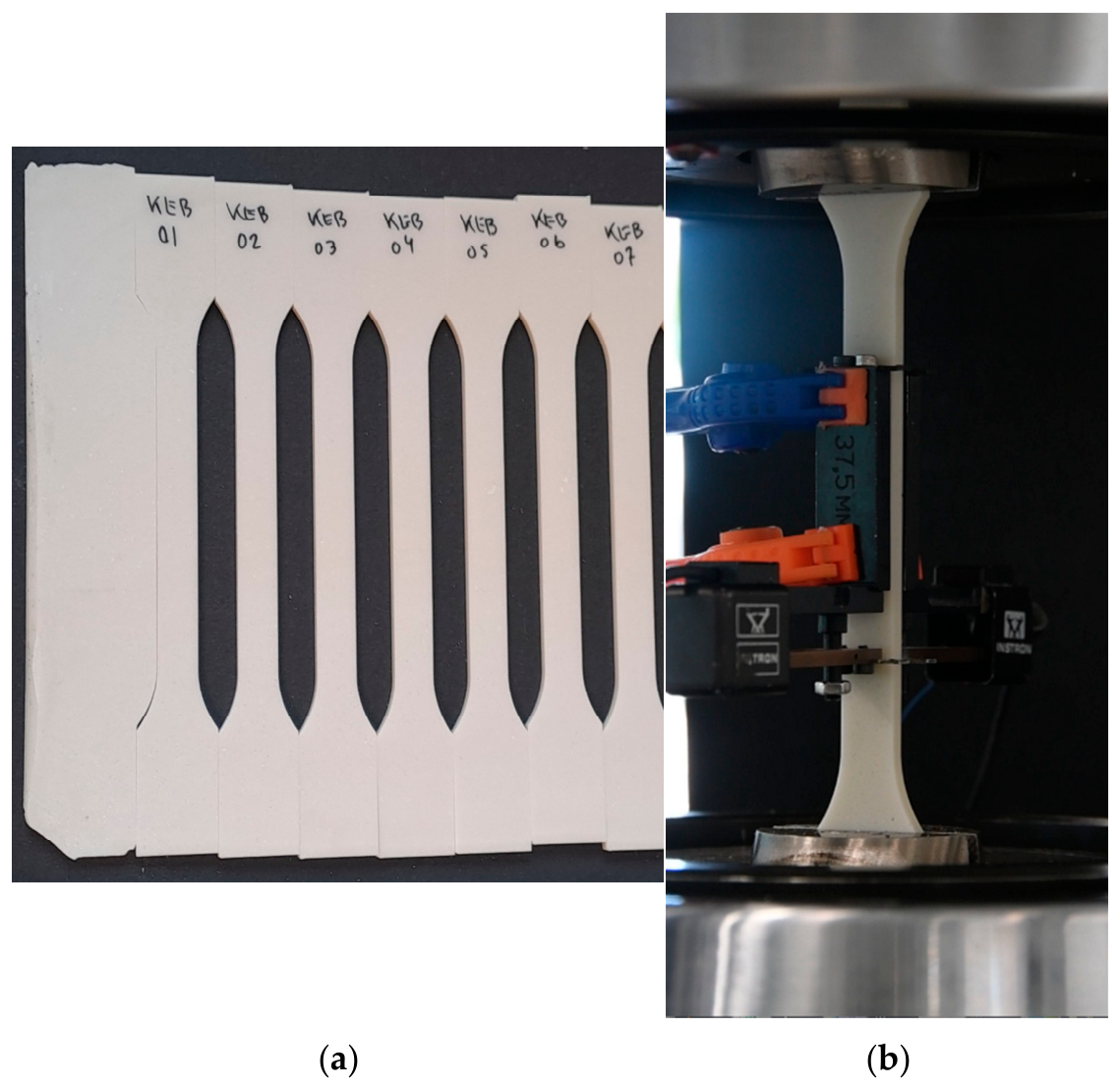
For the static tensile tests on the matrix material, seven samples were tested following the standard ISO 527-2 [44]. The Universal Testing Machine (UTM) used was an Instron 8874 (Instron, Norwood, MA, USA) equipped with a 10 kN load cell. The samples were dogbone-shaped with a width of 10 mm and an average thickness of 3.32 mm, in accordance with ISO 527-2 (Figure 19a). The samples were carefully aligned between the clamps. The test speed was 2 mm/min. The gauge length was 50 mm, while the strain was measured using two extensometers per sample (Figure 19b). The temperature was 21.2 ± 0.1 °C and the humidity was 38%.

Figure 19. (a) The seven samples, cut from the matrix plate, before tensile testing; (b) a matrix sample, subjected to tensile testing, including the two back-to-back mounted extensometers, is shown.

The experimental data were exported as text files and post-processed through a Python script (Python 3.11). The tensile stress–strain curves were computed from the recorded data. Each curve was then linearly interpolated and pointwise averaged to obtain a representative mean stress–strain curve. The von Mises stress–strain curve was also calculated for subsequent analysis.

3.2.2. Matrix Shear Testing

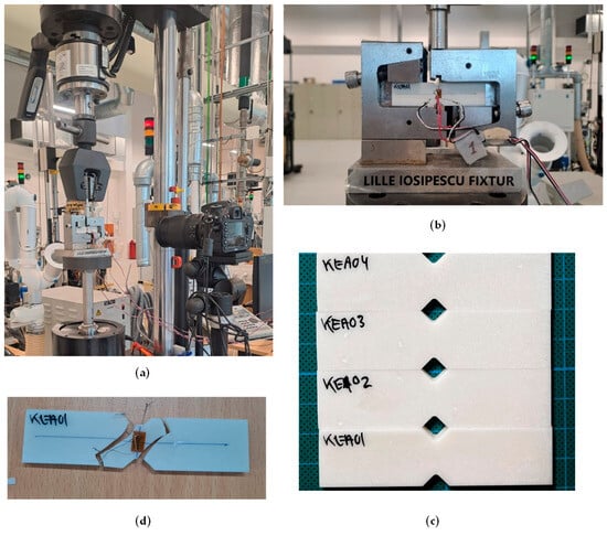
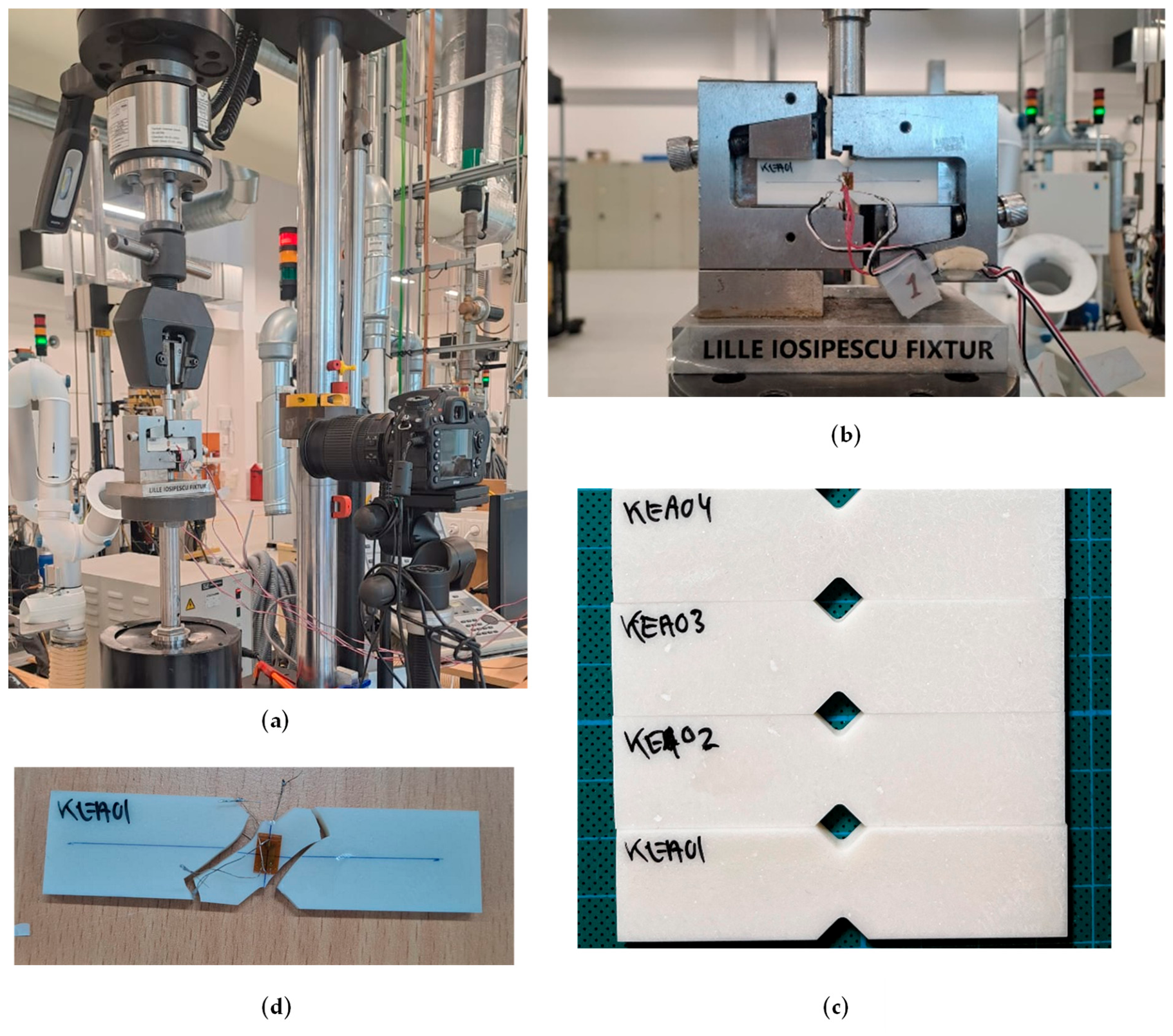
Shear testing was performed on four samples cut from the matrix plate (Figure 20c). The geometry of the samples followed the ASTM D5379 standard [45]. Τhe sample’s width and thickness were, on average, 11.46 mm and 3.46 mm, respectively. A 50 kN load cell (Instron 1362, Instron, Norwood, MA, USA) was used. To perform the shear testing (Figure 20a), the Iosipescu fixture was attached to the machine (Figure 20b). Strain was measured using two strain gauges per sample: one on the front (Figure 20d) and one on the back. The strain gauges used were V-shaped, of type 1-XY21-1.5/350, consisting of two measuring grids arranged at ±45°. Each grid had a length of 1.5 mm and a nominal resistance of 350 Ω. The test speed was 1 mm/min. During the measurements, the temperature was 22.1 ± 0.1 °C, while the humidity was 58%.

Figure 20. (a) The setup of the shear tests of the matrix samples; (b) the Iosipesu fixture used for the testing; (c) the four matrix samples before the failure; (d) Sample 1 after the failure. The strain gauge used is shown on the sample.

The experimental data were recorded in .txt format and post-processed using a Python script. Specifically, the shear strain was derived from the ±45° strain-gauge signals. The absolute values were used to avoid sign cancelation, and the shear strain was defined as the average of the two signals. The shear stress was calculated by dividing the applied load by the nominal shear area at the notch section. Therefore, the shear stress–strain curves were obtained, and the corresponding mean response was calculated. In addition, von Mises equivalent stress–strain curves were derived.

3.2.3. Ramberg–Osgood Material Model Parameters Determination

For the determination of the fitting parameters ${\sigma }_{0,m}$ and $n_m$, a Python code was developed. The fitting was not trivial, since the Ramberg–Osgood material model formula (Equation (3)) is an f(y), instead of a f(x), equation, as well as the fact that the two unknown fitting parameters were coupled, with $n_m$ being an exponent and ${\sigma }_{0,m}$ appearing within that exponent.

The code was developed not only for this case but also for general data fitting in the Ramberg–Osgood material model. The main inputs needed were the material’s Young’s modulus and experimentally obtained stress–strain data. The user should also specify whether the strain is expressed as a percentage and whether the data file includes a header. For the fitting parameters, bounds were set to yield a wide range of positive values to avoid unrealistic solutions. The Python script used for the Ramberg–Osgood fitting procedure is available in [19].

The code is described by the following steps:

• Step 1: Read the experimentally acquired stress–strain data, either from a .csv or an Excel file, and return a list of the corresponding stress–strain pairs.
• Step 2: A third-degree Bezier curve was created using the extracted stress–strain pairs as control points. The reason for this was to smooth the experimental results. The step was 0.01.
• Step 3: A fourth-degree polynomial equation was fit and used to describe the Bezier curve.
• Step 4: The derivative of the polynomial equation was calculated, and the pair of points that is related to the derivative being equal to zero was found (for positive pairs above zero). In this way, a potential change in the polynomial, and thus the experimental curve’s trend (due to the actual finishing of the test or due to fitting a viscoelastic material), would be noticed. It should be noted that a flag captures any pair of values that is related to a zero derivative and is higher than the largest pair of points derived from the Bezier curve.
• Step 5: The first and last points, between which the Ramberg–Osgood material model will be optimized to fit the experimental data, are defined. The initial point is (0,0), and the last one is either the pair of points related to zero derivative or the highest pair of points derived from the Bezier curve.
• Step 6: Use of the optimization algorithm to determine the two fitting parameters. Initially, the two optimization objectives are combined into a single objective. The first is to minimize the distance between the polynomial curve (representing the experimental data) and the fitted curve of the Ramberg–Osgood material model. It should be noted that since the polynomial function is a g(x) and the Ramberg–Osgood material model is described by a f(y), for each strain value x considered, the g(x) = y is calculated, and then this serves as an input for the f(y), meaning that the x_{Ramberg-Osgood} = f(y) = f(g(x)).

The second objective is to minimize the distance between the last points of the two aforementioned curves to avoid a fit that diverges at the end of the polynomial curve. The weights of the two objectives can be adjusted; the default is a = 0.95 for the first objective and b = 0.05 for the second. The equation to describe the combined objective is

$$a·\left(\mathrm{f}\mathrm{i}\mathrm{r}\mathrm{s}\mathrm{t} \mathrm{o}\mathrm{b}\mathrm{j}\mathrm{e}\mathrm{c}\mathrm{t}\mathrm{i}\mathrm{v}\mathrm{e}\right)+b·(\mathrm{s}\mathrm{e}\mathrm{c}\mathrm{o}\mathrm{n}\mathrm{d} \mathrm{o}\mathrm{b}\mathrm{j}\mathrm{e}\mathrm{c}\mathrm{t}\mathrm{i}\mathrm{v}\mathrm{e})$$

(17)

The optimization algorithm used was the limited-memory Broyden–Fletcher–Goldfarb–Shanno one. In this algorithm, in addition to the combined objective, bounds on the fitting parameters and initial guesses for their values are considered. The optimization algorithm returns the values of the two fitting parameters.

3.3. Composite

3.3.1. X-Ray CT Scanning and Reconstruction of the Composite Samples

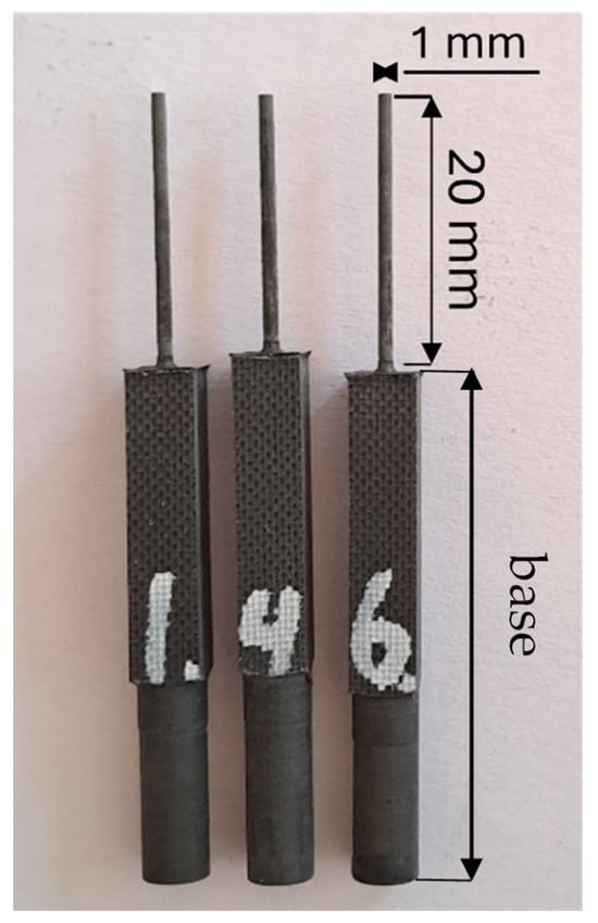
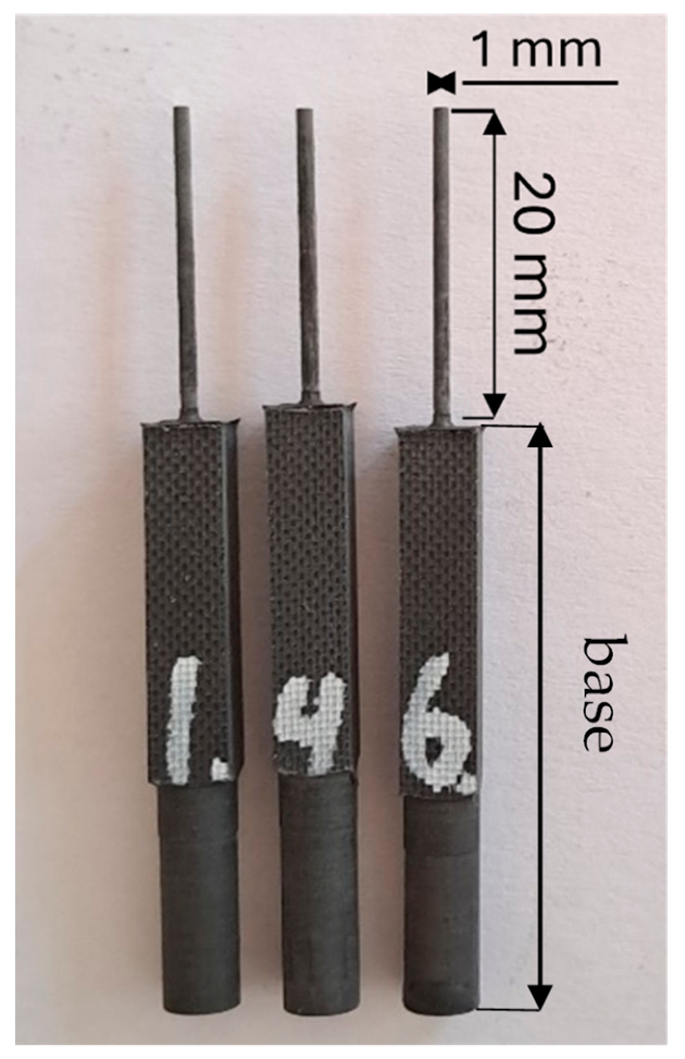
The three samples that were subjected to X-ray CT scanning are shown in Figure 21. Each sample was cut to include a base. This base was essential for securely positioning the samples during scanning. The sample length was 20 mm, and the diameter was 1 mm.

Figure 21. The X-ray scanned samples, cut from carbon fiber unidirectional pultruded profiles. The base of the samples is visible.

Image reconstruction of tomographic data acquired via X-ray scanning was performed using the open-source Python toolbox TomoPy [46] within the DanMAX reconstruction pipeline. TomoPy uses the Gridrec algorithm [47], which is based on discrete Fourier transforms of data. The reconstruction workflow included flat-field and dark-field corrections using averaged flat and dark images, phase retrieval, and outlier removal. The projections were aligned based on the experimental setup parameters. Projection unfolding was applied to achieve a larger field of view. The reconstruction was done with the in-house DanMAX pipeline. Further details can be found in [48].

3.3.2. Composite Compression Testing

The static compression tests for the composite material were carried out on three sets of dogbone-shaped samples, A, B, and C. Sets A and C each consisted of six samples, while set B consisted of five. The dimensions of the tested samples are shown in Table 6. For all samples, the total length was 195.0 mm, and the distance between the tabs was 13.0 mm.

Table 6. Dimensions of the composite samples used for compressive testing, along with the calculated values of the Young’s modulus and the strength. The average values for each sample set, the corresponding standard deviation [%], and the overall average are presented.

	Width	Thickness	Young’s Modulus, EC	Strength, σC
Set A	6.12 mm	5.01 mm	133.2 GPa	1160.7 MPa
Standard deviation [%]	0.1	0.1	2.1	6.8
Set B	6.15 mm	5.04 mm	132.8 GPa	1154.2 MPa
Standard deviation [%]	0.0	0.2	2.8	6.7
Set C	6.13 mm	4.98 mm	137.5 GPa	1348.7 MPa
Standard deviation [%]	0.1	0.0	1.3	3.0
Overall average	6.14 mm	5.01 mm	134.5 GPa	1221.2 MPa
Standard deviation [%]	0.2	0.4	2.5	9.0

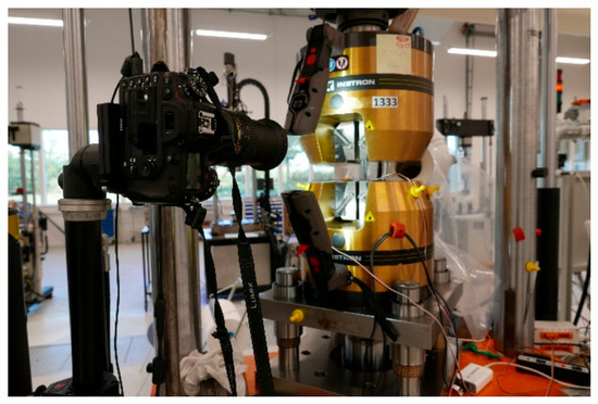
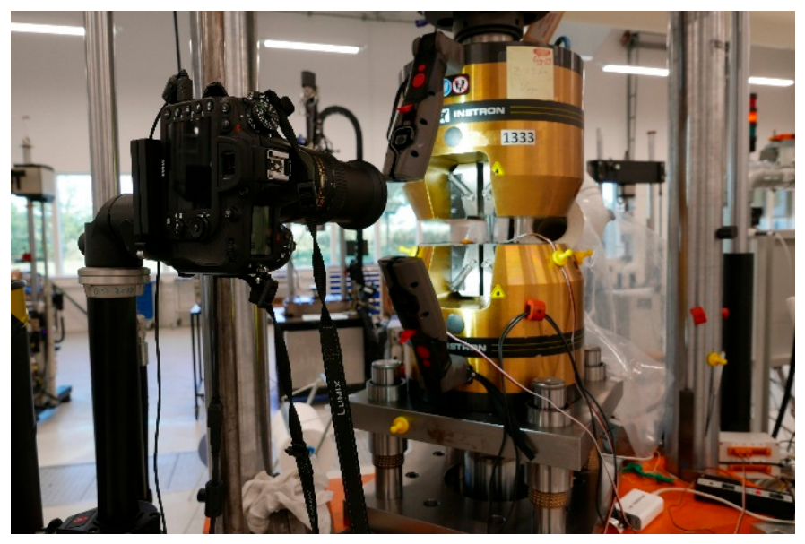
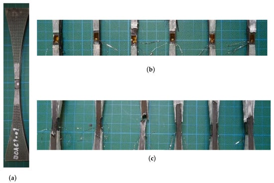
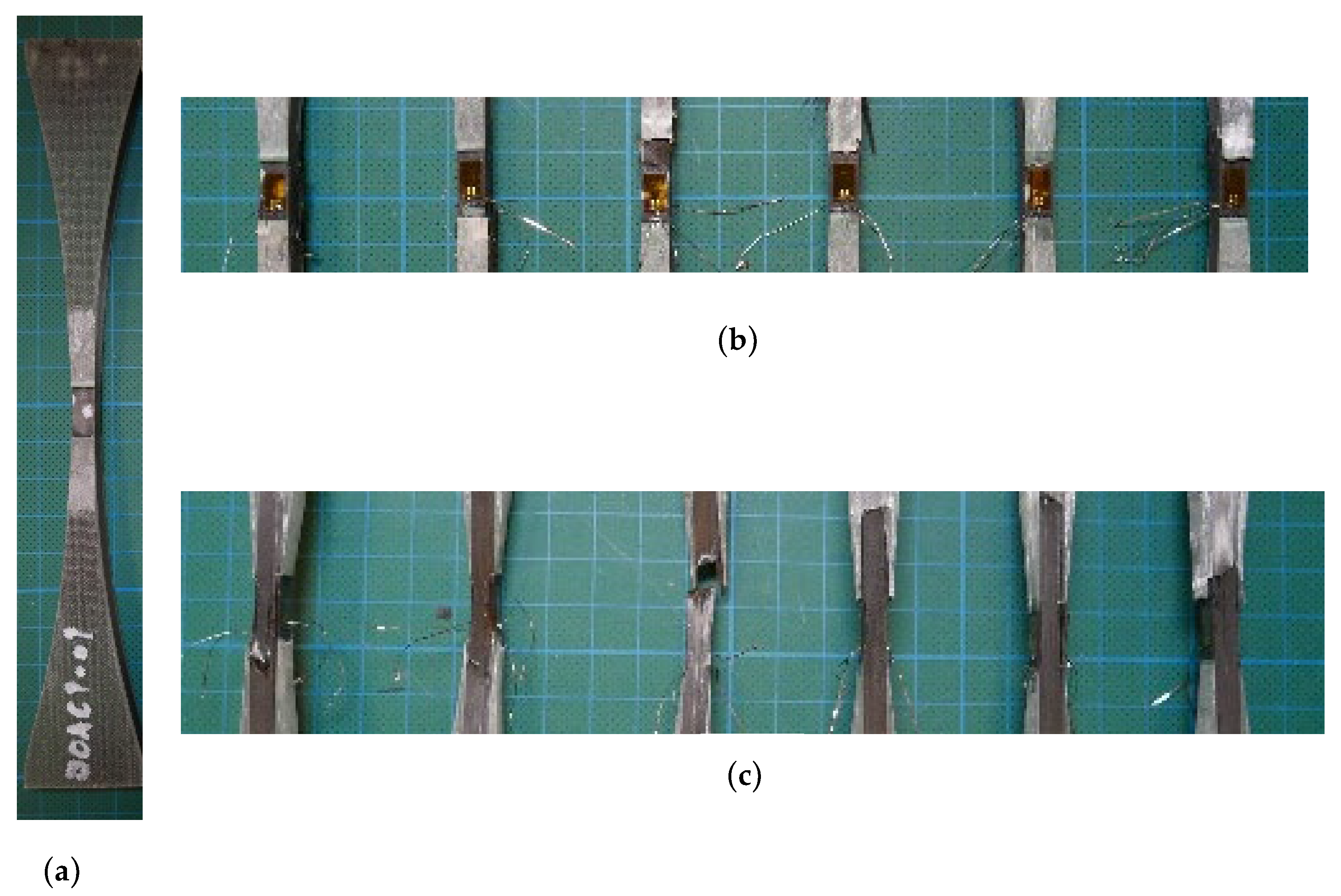
A UTM (Instron 1333, Instron, Norwood, MA, USA) was used with a 250 kN load cell. The samples were carefully aligned between the upper and lower clamp to avoid sample misalignment. The test speed was 1 mm/min. The setup for the compression test is shown in Figure 22. Two strain gauges were used per sample. Their length was 3 mm and their type HBK 1-LY11-3/350. Pictures of the samples before and after the compression test (Figure 23), of the setup, as well as a video of the test, were captured. The temperature was 22.0 ± 0.1 °C and the humidity was 56%.

Figure 22. The compression test setup on the UTM, with the sample clamped. Image used in [13].

Figure 23. (a) A sample of set A before the compression test without strain gauges; (b,c) the gauge section of all samples from set A after the compression test.

Through the compression tests, the experimental data were recorded to obtain the stress–strain curves for each sample. To compute the strain, the signals of the two strain gauges per sample were averaged. The Young’s modulus of the composite, E_C, was calculated for a strain range of [0.05–0.25]%, according to ISO-14126 [49]. The strength, σ_C, was also found, which was the maximum stress value. The results are presented in Table 6. The differences in compressive strength between sets A, B, and C may be related to the corresponding variations in fiber volume fraction and porosity reported in Section 2.3.3 and Table 4, where set C shows a slightly higher fiber volume fraction and lower porosity compared to sets A and B.

3.3.3. Fiber Content Analysis Through the Burn-Off Method

To determine the fiber volume fraction, the burn-off method was used. In addition to the volume content, the fiber and matrix weight fractions, composite density, and porosity were determined. The first step was cutting three groups of coupons from the pultruded profiles corresponding to the X-ray scanned samples. The first and third groups each had five coupons, while the second had three. The coupons’ cross-section was 15 mm × 15 mm, ensuring a mass greater than 1 g, as shown in Table 4, which, according to ASTM D3171-22 [34], is the minimum required for the void content determination. Attention was paid during coupon cutting to avoid introducing any potential defects into the material. The coupons were cleaned of any loosely attached material, such as cutting fragments, dust, and protruding fibers, to prevent any material from falling off during analysis. Then, the coupons were dried for at least 16 h under vacuum at room temperature to prevent absorbed humidity from affecting the measurements. The drying process was performed in a vacuum oven at a typical pressure of 0.7 mbar.

Τhe crucibles that would be used were annealed in a muffle furnace at 625 °C for at least one hour, and then cooled down in a desiccator containing a moisture-absorbing material, for around one hour at room temperature. It should be mentioned that after their annelation, the crucibles were handled with tongs or tweezers, so that they would not become polluted by touching them. The same careful handling was applied to the dried coupons.

The next step was to weigh the coupons on an analytical balance. After that, the coupons were sealed in a fume cabinet to prevent them from absorbing water during the measurements. The sealing occurred on the coupons’ surface, using a paraffin wax in petroleum ether solution. When the coupons were dry, they were weighed again on the analytical balance.

The density of the coupons was measured through Archimedes’ principle, according to which the buoyancy of an immersed object is equal to the mass of the displaced medium. Therefore, the coupons were immersed in water and weighed. The setup used for these measurements consisted of a beaker filled with boiled demineralized water, a sample holder holding the coupon immersed in water, and a balance. The water temperature, T_w, was given in [°C] and recorded because water density depends on it. For every case, the temperature was 21.1 °C. The water density, ρ_w, was described through the following equation:

$${\rho }_w=\left(1-{\displaystyle \frac{49.2539}{\mathrm{1,000,000}}}\right)+{\displaystyle \frac{T_w}{100·(0.004514 - \frac{T_w}{100·(0.07299 -\frac{T_w}{100·0.033738})}}} \left[{\displaystyle \frac{\mathrm{g}}{{\mathrm{c}\mathrm{m}}^3}}\right]$$

(18)

Therefore, the composite material’s density, ρ_c, was found to be

$${\rho }_c={\displaystyle \frac{m_c·{\rho }_w}{m_{c,s}-m_{c,w}-\frac{{\rho }_w·(m_{c,s}-m_c)}{{\rho }_s}}}$$

(19)

where m_c is the mass of the composite coupon considered, m_c,s the mass of the same coupon after sealing, and m_c,w the mass of the coupon in the water. The sealing density, ρ_s, was already known.

Then, the coupons were weighed in water, and the empty crucibles were weighed afterward. The coupons were placed in crucibles and heated in a muffle furnace to 625 °C to burn off the matrix. After complete removal of the matrix, the crucibles, containing only carbon fibers, were placed in a desiccator containing a moisture-absorbing material at room temperature. In this way, they were kept dry while cooling for about one hour. The crucibles containing the carbon fibers were then weighed. The calculations used the following equations:

$$m_f=m_{cruc with fibers}-m_{cruc}$$

(20)

where m_f is the mass of the fibers, m_{cruc with fibers} the mass of the crucible containing the fibers and m_cruc the mass of the empty crucible.

$$W_f={\displaystyle \frac{m_f}{m_c}}$$

(21)

$$W_m=1-W_f$$

(22)

where W_f and W_m are the fiber and matrix weight content, respectively.

$$V_f={\displaystyle \frac{{\rho }_c·W_f}{{\rho }_f}}$$

(23)

$$V_m={\displaystyle \frac{{\rho }_c·W_m}{{\rho }_m}}$$

(24)

$$V_p=1-V_f-V_m$$

(25)

where V_f and V_m are the volume contents and ρ_f and ρ_m are the already known values of the density for the fiber and the matrix, respectively. The volume content of porosity is annotated as V_p.

3.3.4. Fiber Volume Fraction Through SEM Image Analysis

A sample acquired from the same pultruded composite material was used for scanning electron microscopy (SEM) to determine the fiber volume fraction, using the method developed by Mikkelsen et al. [10]. The reader is referred to that work for details and access to the related data. The determination of fiber volume fraction by SEM was preferred over X-ray CT due to the higher spatial resolution and better contrast between fibers and matrix, enabling the more accurate segmentation of fiber cross-sections. The basic steps of the method are presented below. The method was developed to determine the fiber orientation fraction across different composite bundles in a single SEM image, but it can also be used for a single case. The SEM image shown in Figure 13 was examined. The SEM instrument used was the Phenom XL G2 from Thermo Fisher Scientific (Waltham, MA, USA), equipped with a special holder named XL Manual Height. The acquisition and stitching of large images were performed using Maps Software version 3.32. After stitching, a single representative SEM image of the composite cross-section was acquired for the determination of the fiber volume fraction.

The first step of the method is performed using the *BundlesAnalysis.m MATLAB R2022b code, where * denotes the name of the SEM downsized image file. The SEM image, in TIFF format, serves as input to the code and, via the bundle_outlining_gui function, is segmented and saved. Apart from a thin zone near the material boundaries, the entire cross-section was used for segmentation.

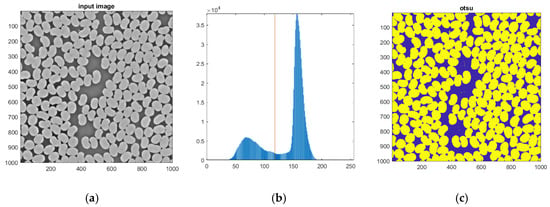
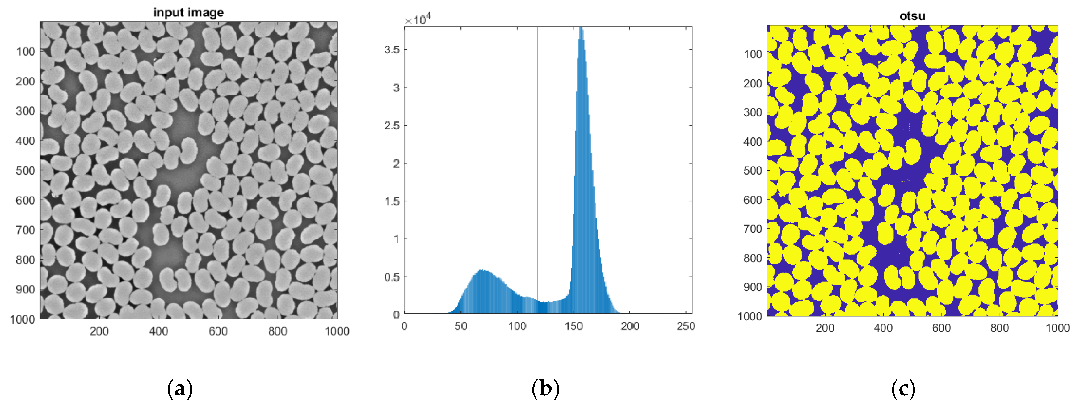
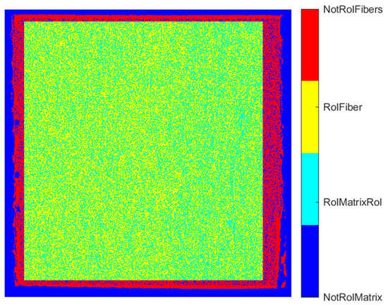
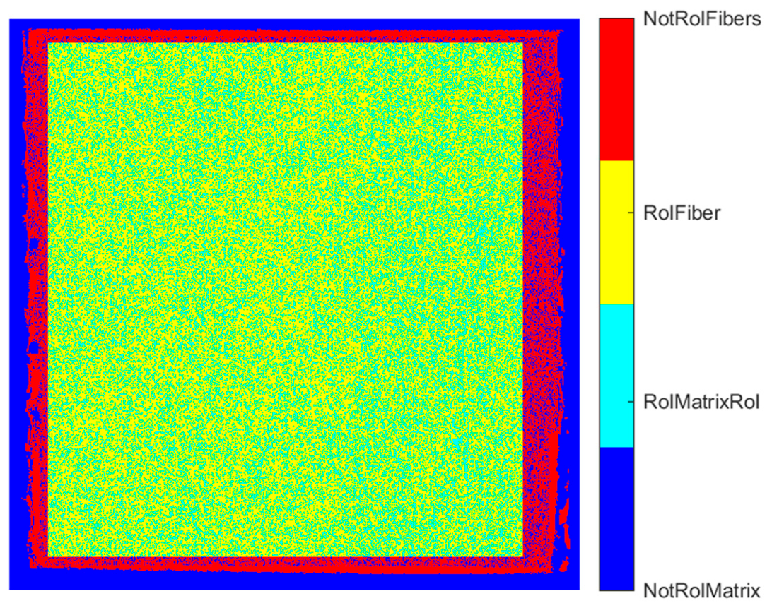
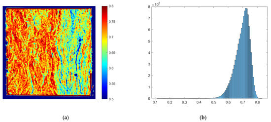
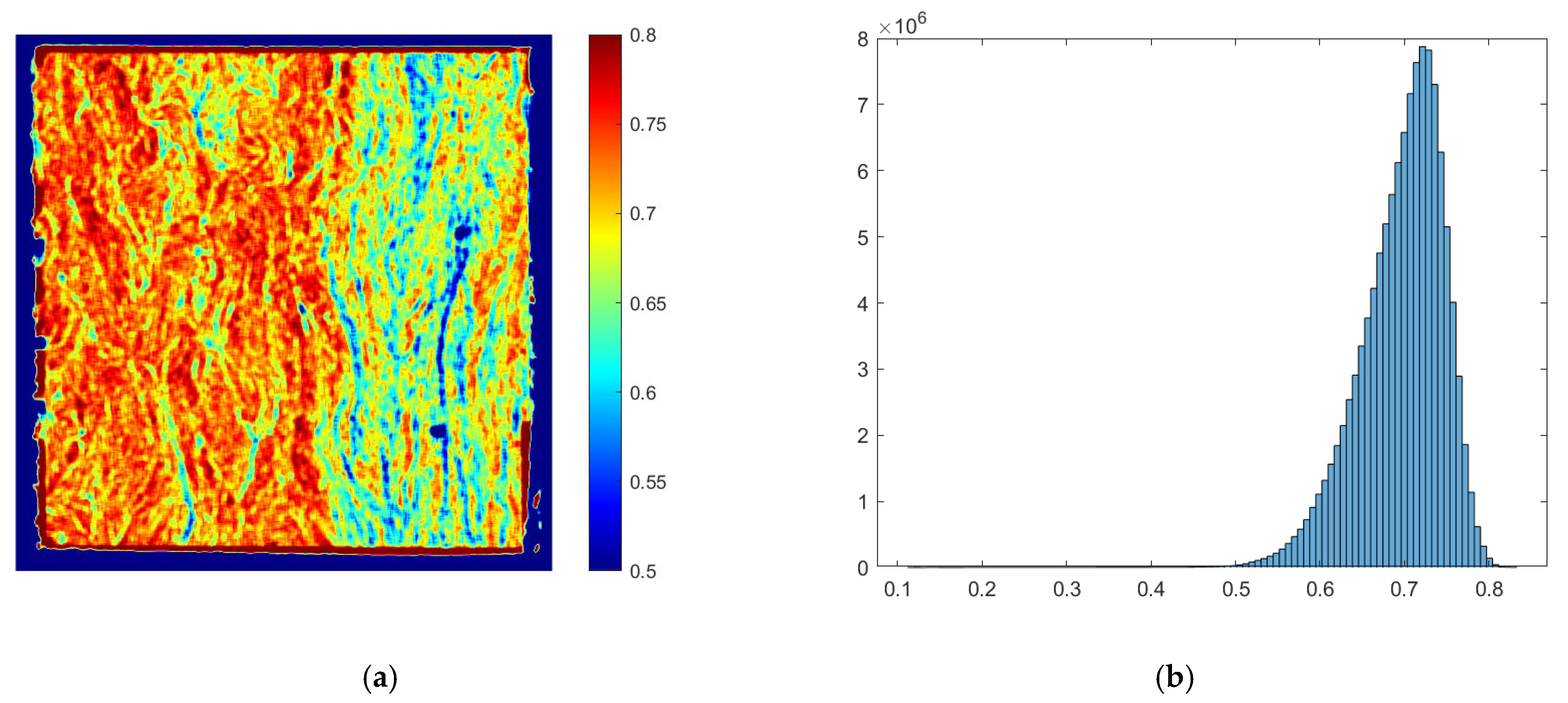
The next step was the use of the *.m script. Initially, a central 1000 × 1000-pixel region of the SEM image was automatically selected (Figure 24a) to determine the Otsu threshold value [50], which, in this case, was 118. The pixel intensity histogram, along with the Otsu threshold, is shown in Figure 24b, while Figure 24c shows the examined region after binarization. Then, the region of interest for calculating the fiber volume fraction was selected from the entire SEM image. As shown in Figure 25, the region of interest was the entire cross-section of the sample, except for the area near the borders. Using this approach, the global fiber volume fraction determined from the SEM image was 69.8%, whereas the burn-off technique yielded an average volume fraction of 65.1%. The difference between the two values is primarily due to the SEM image segmentation, which depends on the Otsu threshold. As shown in Figure 24b, the pixel intensity histogram does not exhibit a well-defined minimum between the fiber and matrix intensity peaks, making the segmentation, and consequently the calculated fiber volume fraction, sensitive to small changes in the threshold value. Therefore, the measurement acquired through the burn-off method is considered the more reliable estimate of the global fiber volume fraction. Nevertheless, the SEM-based approach is essential because it enables the determination of the distribution of the local fiber volume fraction, as shown in Figure 26a, which cannot be obtained with the burn-off technique. In Figure 26b, the corresponding histogram is shown. The averaging box, or kernel size, used for the calculation of the local volume fraction was (5 × fiber diameter)², where the fiber diameter was the mean, or d_f = 7.5 μm.

Figure 24. (a) The 1000 × 1000 pixels cropped SEM image for the determination of the Otsu threshold; (b) the histogram of the pixel intensity, with the Otsu threshold annotated; (c) the cropped SEM image after binarization according to the Otsu threshold.

Figure 25. The region of interest (RoI) for calculating the fiber volume fraction was 69.8%. The different colors indicate the fiber and the matrix at the region of interest, as well as the fiber and the matrix outside of it. The region of interest is split into the fiber region of interest (RoIFiber) and the matrix region of interest (RoIMatrixRoI).

Figure 26. (a) The contour plot of the local fiber volume fraction, based on the SEM image; (b) the histogram of the local fiber volume fraction distribution.

By comparing the contour plot with the examined SEM image, and particularly the areas that are more or less dense on fibers, it can be concluded that the differences in the local fiber volume fraction have been well captured.

3.3.5. Determination of the Fiber Orientation Through Structure Tensor Analysis

The fiber orientation was determined using structure tensor analysis, which is a mathematical image analysis method widely used by researchers [11,12,38,51,52]. The method was implemented in Python, using the structure tensor package. The input for the three-dimensional structure tensor was a digital subvolume of the scanned CT sample. The method is applied at each voxel of this subvolume, computing the local gradients of greyscale intensity. Individual fiber segmentation was not performed because the available CT resolution and contrast do not permit the straightforward, robust identification of single fibers throughout the volume. Then, the structure tensor, which is a 3 × 3 matrix, is constructed for each voxel neighborhood as follows:

$$\mathit{S}=\sum \nabla \mathit{V}{(\nabla \mathit{V})}^T$$

(26)

where $V$ is the volumetric data of voxel intensities, and $\nabla \mathit{V}= {[V_x V_y V_z]}^T$ represents the intensity gradients according to the coordinate system used.

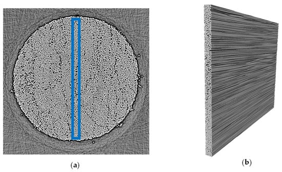
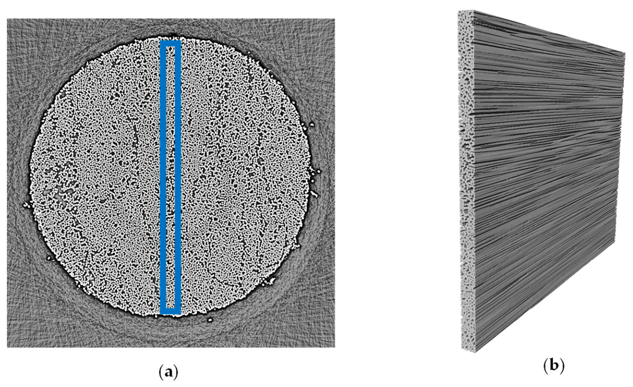
The first step was to create the three-dimensional sample subvolume used for the structure tensor analysis. The scanned images (Figure 12) were subjected to histogram equalization to enhance the greyscale contrast between the fibers and the matrix. Using histogram equalization, the pixel intensities were adjusted to span the full greyscale range (0–255). The data size for a single sample’s scanned images was 39 GB. Since only one slice was needed for the two-dimensional model [13], and to make the method more computationally efficient, the images were cropped (Figure 27). The cropped images were stacked to create a three-dimensional subvolume of the sample with a thickness of 100 slices, as shown in the aforementioned Figure. This thickness was chosen to ensure computational efficiency while being suitable for the structure tensor analysis. The distance between the slices corresponds to the voxel size.

Figure 27. (a) One slice from the X-ray scanning, after histogram equalization. The blue rectangle represents the area of the image that was cropped. (b) The digital subvolume, created by stacking the cropped images. [13].

In this work’s Python code, after providing the sample’s digital subvolume as input in the NIfTI (Neuroimaging Informatics Technology Initiative) file format, which is widely used for storing large volumetric datasets acquired from X-ray scanning, the structure tensor parameters were calculated. These parameters are the integration scale, ρ, and the noise scale, σ. According to [11], they are calculated as follows:

$$\rho = {\displaystyle \frac{d_f}{voxel size}}$$

(27)

$$\sigma ={\displaystyle \frac{\rho }{2}}$$

(28)

where d_f is the average fiber diameter. The integration scale defines the size of the neighboring area around each voxel, while the noise scale filters out high-frequency noise. The structure tensor Python package used in the presented case requires only these two parameters to compute the structure tensor. The Gaussian kernel window, K_ρ, is computed from the integration and the noise scale, and used to average the gradient information in the neighborhood of each voxel. The structure tensor is computed as follows:

$$\mathit{S}=K_{\rho }\left(\nabla {\mathit{V}}_{\mathit{\sigma }}{\left(\nabla {\mathit{V}}_{\mathit{\sigma }}\right)}^T\right)$$

(29)

where $\nabla {\mathit{V}}_{\mathit{\sigma }}$ represents the intensity gradients.

The structure tensor is then subjected to eigen decomposition, resulting in three positive eigenvalues, ${\lambda }_1\le {\lambda }_2\le {\lambda }_3$, for each voxel. The smallest eigenvalue, λ₁, corresponds to the smallest change in voxel greyscale intensity. The eigenvector corresponding to each eigenvalue, ${\mathit{r}}_1,{\mathit{r}}_2$ and ${\mathit{r}}_3$, can be calculated; these describe the predominant fiber orientations. Considering that the smallest change in voxel intensity indicates the dominant fiber orientation, the eigenvector that is related to the smallest eigenvalue, ${\mathit{r}}_1$, is the one describing the dominant fiber orientation. The components of the eigenvector ${\mathit{r}}_1$ are described as $r_{1,x}, r_{1,y}$ and $r_{1,z}$, depending on the axis they refer to.

Since the aforementioned eigenvectors indicate the dominant direction, and not orientation, there might be two neighboring voxels having the same orientation but opposite directions. During fiber orientation angle calculation, this may lead to an inaccurate fiber distribution. To avoid this, all eigenvectors are aligned across the positive z-axis (the axis across the longitudinal direction of the fibers), as follows:

$${\mathit{r}}_{1,R}=sign\left(r_{1,z}\right){\mathit{r}}_1$$

(30)

with ${\mathit{r}}_{1,R}$ representing the rotated eigenvector. In this work, the subscript R is omitted; thus, ${\mathit{r}}_1= {\mathit{r}}_{1,R}$, with its z component described as $r_{1,z}$.

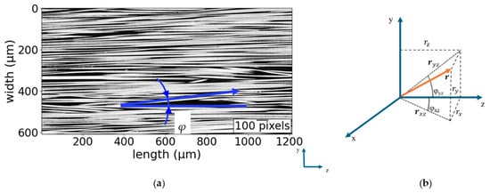
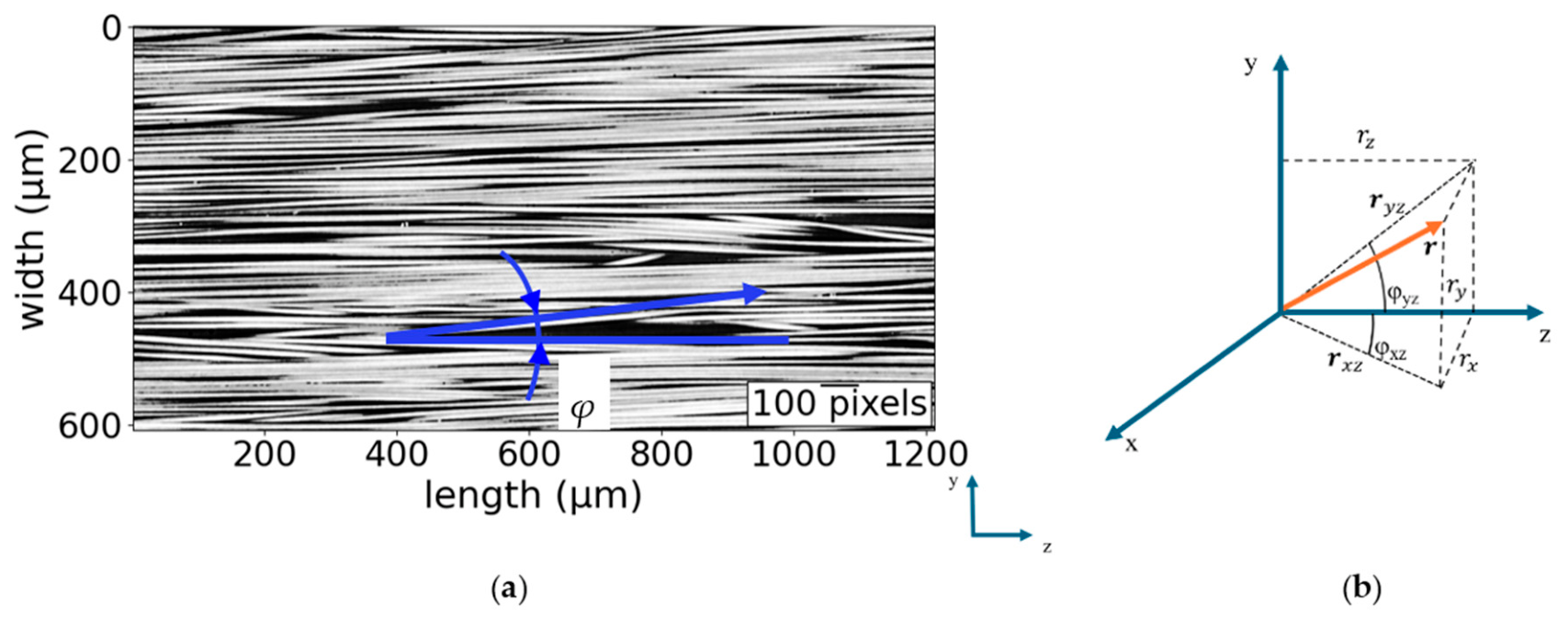
To describe the orientation, the elevation angle, φ, was calculated. The elevation angle is the angle formed between the examined fiber’s orientation projection on the plane of interest (xz- or yz-plane) and a theoretical fiber perfectly aligned across the z axis, as can be seen in Figure 28. The elevation angle was calculated for the examined plane as follows:

$${\phi }_{yz}=\arctan \left({\displaystyle \frac{r_{1,y}}{r_{1,z}}}\right)$$

(31a)

$${\phi }_{xz}=\arctan \left({\displaystyle \frac{r_{1,x}}{r_{1,z}}}\right)$$

(31b)

with the z-axis across the longitudinal direction of the fibers. As an additional step that is essential for considering the fiber orientation variation during numerical modeling, the matrix of the elevation angles for an examined slice was saved as an NPZ (NumPy compressed archive, where NumPy stands for Numerical Python) file. This format allows this data to be used as input for finite element simulations.

Figure 28. (a) An examined slice of the yz-plane, showing the longitudinal direction of the fibers and extracted from the digital subvolume, along with the depiction of the elevation angle φ, for a fiber. (b) The eigenvector ${\mathit{r}}_1$ in relation to the coordinate system used, and along with its components and projections on yz- and xz-planes. Note that the subscript 1 is omitted [13].

References

- Sinchuk, Y.; Kibleur, P.; Aelterman, J.; Boone, M.N.; Van Paepegem, W. Variational and deep learning segmentation of very-low-contrast X-ray Computed tomography images of carbon/epoxy woven composites. Materials 2020, 13, 936. [Google Scholar] [CrossRef] [Scilit]
- Tang, C.; Zou, J.; Xiong, Y.; Liang, B.; Zhang, W. Automatic reconstruction of closely packed fabric composite RVEs using yarn-level micro-CT images processed by convolutional neural networks (CNNs) and based on physical characteristics. Compos. Sci. Technol. 2024, 252, 110616. [Google Scholar] [CrossRef] [Scilit]
- Can Zehni, O.; Xu, J.; Lowe, T.; Whitehouse, E.; Ataş, A. Continuous carbon fibre reinforced 3D-printed composites: Impact damage and compression after impact (CAI) performance. Compos. Part A Appl. Sci. Manuf. 2025, 198, 109097. [Google Scholar] [CrossRef] [Scilit]
- Kim, S.Y.; Shim, C.S.; Sturtevant, C.; Kim, D.D.W.; Song, H.C. Mechanical properties and production quality of hand-layup and vacuum infusion processed hybrid composite materials for GFRP marine structures. Int. J. Nav. Archit. Ocean Eng. 2014, 6, 723–736. [Google Scholar] [CrossRef] [Scilit]
- Plappert, D.; Ganzenmüller, G.C.; May, M.; Beisel, S. Mechanical properties of a unidirectional basalt-fiber/epoxy composite. J. Compos. Sci. 2020, 4, 101. [Google Scholar] [CrossRef] [Scilit]
- Emerson, M.J.; Dahl, V.A.; Conradsen, K.; Mikkelsen, L.P.; Dahl, A.B. A multimodal data-set of a unidirectional glass fibre reinforced polymer composite. Data Brief 2018, 18, 1388–1393. [Google Scholar] [CrossRef] [Scilit] [PubMed]
- Liu, F.; Grotz, L.; Cui, Y.; Kirane, K. Experimental dataset on the in-plane tensile, shear, and compressive properties of a carbon-epoxy twill woven composite. Data Brief 2022, 45, 108650. [Google Scholar] [CrossRef] [Scilit] [PubMed]
- Kumar, R.; Mikkelsen, L.P.; Lilholt, H.; Madsen, B. Weibull parameters determined from a comprehensive dataset of tensile testing of single carbon fibres. Data Brief 2024, 55, 110717. [Google Scholar] [CrossRef] [Scilit] [PubMed]
- Ramberg, W.; Osgood, W.R. Description of Stress-Strain Curves by Three Parameters; Technical Note No. 902; National Advisory Committee for Aeronautics: Washington, DC, USA, 1943. [Google Scholar]
- Mikkelsen, L.P.; Fæster, S.; Dahl, V.A. Dataset for scanning electron microscopy based local fiber volume fraction analysis of non-crimp fabric glass fiber reinforced composites. Data Brief 2023, 48, 109058. [Google Scholar] [CrossRef] [Scilit] [PubMed]
- Jeppesen, N.; Mikkelsen, L.P.; Dahl, A.B.; Christensen, A.N.; Dahl, V.A. Quantifying effects of manufacturing methods on fiber orientation in unidirectional composites using structure tensor analysis. Compos. Part A Appl. Sci. Manuf. 2021, 149, 106541. [Google Scholar] [CrossRef] [Scilit]
- Karamov, R.; Martulli, L.M.; Kerschbaum, M.; Sergeichev, I.; Swolfs, Y.; Lomov, S.V. Micro-CT based structure tensor analysis of fibre orientation in random fibre composites versus high-fidelity fibre identification methods. Compos. Struct. 2020, 235, 111818. [Google Scholar] [CrossRef] [Scilit]
- Mageira, P.; Poulios, K.; Andreasen, J.W.; Dahl, V.A.; Gundlach, C.; Mikkelsen, L.P. Compression strength prediction of unidirectional carbon fiber composites using a mesh independent homogenization model and real fiber orientation distribution. Eur. J. Mech. A/Solids, 2026; submitted.
- Mageira, P.; Poulios, K.; Andreasen, J.W.; Dahl, V.A.; Mikkelsen, L.P. Experimental and Numerical Compression Analysis of 3D X-Ray CT Scanned Unidirectional Pultruded Carbon Fiber Composites. In Proceedings of the ICCM International Conferences on Composite Materials, Baltimore, MD, USA, 4 August 2025. [Google Scholar]
- Mageira, P.; Poulios, K.; Andreasen, J.W.; Dahl, V.A.; Mikkelsen, L.P. From 3D X-ray CT scans to mesh-independent numerical compressive strength predictions of unidirectional carbon fiber composites. IOP Conf. Ser. Mater. Sci. Eng. 2025, 1338, 012026. [Google Scholar] [CrossRef] [Scilit]
- Mageira, P.; Gundlach, C.; Mikkelsen, L.P. X-Ray CT Scan Data of Pultruded Carbon Fiber Composite-Sample A; Zenodo: Meyrin, Switzerland, 2026. [Google Scholar] [CrossRef]
- Mageira, P.; Gundlach, C.; Mikkelsen, L.P. X-Ray CT Scan Data of Pultruded Carbon Fiber Composite-Sample B; Zenodo: Meyrin, Switzerland, 2026. [Google Scholar] [CrossRef]
- Mageira, P.; Gundlach, C.; Mikkelsen, L.P. X-Ray CT Scan Data of Pultruded Carbon Fiber Composite-Sample C; Zenodo: Meyrin, Switzerland, 2026. [Google Scholar] [CrossRef]
- Mageira, P.; Mikkelsen, L.P. Dataset of Unidirectional Carbon Fiber Pultruded Composites and Their Constituents (Fibers and Matrix); Zenodo: Meyrin, Switzerland, 2026. [Google Scholar] [CrossRef]
- Mesquita, F.; Bucknell, S.; Leray, Y.; Lomov, S.V.; Swolfs, Y. Large datasets of single carbon and glass fibre mechanical properties obtained with automated testing equipment. Data Brief 2021, 36, 107085. [Google Scholar] [CrossRef] [Scilit] [PubMed]
- Kumar, R.; Mikkelsen, L.P.; Lilholt, H.; Madsen, B. Understanding the mechanical response of glass and carbon fibres: Stress-strain analysis and modulus determination. IOP Conf. Ser. Mater. Sci. Eng. 2020, 942, 012033. [Google Scholar] [CrossRef] [Scilit]
- Huether, J.J.; Liebig, W.V. Investigations of the carbon fibre cross-sectional areas and their non-circularities by means of laser diffraction. IOP Conf. Ser. Mater. Sci. Eng. 2020, 942, 012034. [Google Scholar] [CrossRef] [Scilit]
- Mesquita, F.; Bucknell, S.; Leray, Y.; Lomov, S.V.; Swolfs, Y. Single carbon and glass fibre properties characterised using large data sets obtained through automated single fibre tensile testing. Compos. Part A Appl. Sci. Manuf. 2021, 145, 106389. [Google Scholar] [CrossRef] [Scilit]
- Jaber, A.A.; Abbas, S.A.; Farah, A.A.; Kopeć, K.K.; Alsalik, Y.M.; Tayeb, M.A.; Verghese, N. Effect of Fiber Sizing Levels on the Mechanical Properties of Carbon Fiber-Reinforced Thermoset Composites. Polymers 2023, 15, 4678. [Google Scholar] [CrossRef] [Scilit] [PubMed]
- Hares, J.; Kelly, P.; Battley, M.; Bickerton, S. A friction-based method for measuring the radial compaction response of fibre tows. Compos. Part A Appl. Sci. Manuf. 2025, 188, 108541. [Google Scholar] [CrossRef] [Scilit]
- Tourkantoni, I.; Tserpes, K.; Marinis, D.; Farsari, E.; Amanatides, E. Mechanical Characterization of Carbon Fibers and Their Interfaces Recycled Through Plasma-Assisted Solvolysis Under Different Processing Conditions. Fibers 2025, 13, 158. [Google Scholar] [CrossRef] [Scilit]
- Ji, X.; Wang, C.; Francis, B.A.P.; Chia, E.S.M.; Zheng, L.; Yang, J.; Joshi, S.C.; Chen, Z. Mechanical and Interfacial Properties Characterisation of Single Carbon Fibres for Composite Applications. Exp. Mech. 2015, 55, 1057–1065. [Google Scholar] [CrossRef] [Scilit]
- Ilankeeran, P.K.; Mohite, P.M.; Kamle, S. Axial Tensile Testing of Single Fibres. Mod. Mech. Eng. 2012, 2, 151–156. [Google Scholar] [CrossRef]
- Sullivan, J.L.; Kao, B.G.; Van Oene, H. Shear properties and a stress analysis obtained from vinyl-ester losipescu specimens. Exp. Mech. 1984, 24, 223–232. [Google Scholar] [CrossRef] [Scilit]
- Dominguez-Macaya, A.; Álvarez-Arenas, T.E.G.; Saenz-Dominguez, I.; Tena, I.; Aurrekoetxea, J.; Iturrospe, A. Monitoring the evolution of stiffness during ultraviolet curing of a vinyl ester resin with quasi-normal air-coupled ultrasonic spectroscopy. Polym. Test. 2019, 80, 106112. [Google Scholar] [CrossRef] [Scilit]
- Adams, D.F. The Iosipescu shear test method as used for testing polymers and composite materials. Polym. Compos. 1990, 11, 286–290. [Google Scholar] [CrossRef] [Scilit]
- Korkiakoski, S.; Brøndsted, P.; Sarlin, E.; Saarela, O. Influence of specimen type and reinforcement on measured tension-tension fatigue life of unidirectional GFRP laminates. Int. J. Fatigue 2016, 85, 114–129. [Google Scholar] [CrossRef] [Scilit]
- Rahman, M.A.; Islam, M.Z.; Gibbon, L.; Ulven, C.A.; La Scala, J.J. 3D printing of continuous carbon fiber reinforced thermoset composites using UV curable resin. Polym. Compos. 2021, 42, 5859–5868. [Google Scholar] [CrossRef] [Scilit]
- ASTM D3171–22; Standard Test Methods for Constituent Content of Composite Materials 1. ASTM International, Inc.: West Conshohocken, PA, USA, 2022.
- Shah, S.; Hazell, P.J.; Wang, H.; Escobedo, J.P. Shock response of unidirectional carbon fibre-reinforced polymer composites: Influence of fibre orientation and volume fraction. Compos. B Eng. 2025, 299, 112438. [Google Scholar] [CrossRef] [Scilit]
- Ennis, B.L.; Das, S.; Norris, R.E. Economic competitiveness of pultruded fiber composites for wind turbine applications. Compos. B Eng. 2023, 265, 110960. [Google Scholar] [CrossRef] [Scilit]
- Creighton, C.J.; Clyne, T.W. The compressive strength of highly-aligned carbon-fibre/epoxy composites produced by pultrusion. Compos. Sci. Technol. 2000, 60, 525–533. [Google Scholar] [CrossRef] [Scilit]
- Ferguson, O.V.; Skovsgaard, S.P.H.; Jensen, H.M.; Mikkelsen, L.P. Compressive strength prediction of carbon fiber-reinforced pultruded profiles including realistic volumetric fiber orientations. Eur. J. Mech. A/Solids 2023, 104, 105011. [Google Scholar] [CrossRef] [Scilit]
- Zhang, B.; Pickard, L.R.; Nwuzor, I.C.; Darras, N.S.T.; Wisnom, M.R.; Allegri, G.; Quino, G.; Robinson, P.; Trask, R.S. The experimental investigation of the compressive performance of pultruded rod composite struts. In Proceedings of the ICCM International Conferences on Composite Materials, Baltimore, MD, USA, 8 August 2025. [Google Scholar]
- Madsen, B.; Kumar, R.; Lilholt, H. Vibroscope method for determination of cross-sectional area of glass and carbon fibres–Experiments and analyses. Compos. Part A Appl. Sci. Manuf. 2024, 187, 108447. [Google Scholar] [CrossRef] [Scilit]
- Madsen, B.; Høgsberg, J.; Lilholt, H. Vibroscope method for determination of cross-sectional area of glass and carbon fibres–Theory and further development. Compos. Part A Appl. Sci. Manuf. 2024, 187, 108447. [Google Scholar] [CrossRef] [Scilit]
- Weibull, W. A Statistical Distribution Function of Wide Applicability. J. Appl. Mech. 1951, 18, 293–297. [Google Scholar] [CrossRef] [Scilit]
- Yang, L.; Thomason, J.L. Effect of silane coupling agent on mechanical performance of glass fibre. J. Mater. Sci. 2013, 48, 1947–1954. [Google Scholar] [CrossRef] [Scilit]
- ISO 527-2; Determination of Tensile Properties of Plastics-Test Conditions for Moulding and Extrusion Plastics. International Organization for Standardization (ISO), Inc.: Geneva, Switzerland, 1996.
- ASTM D5379M-19; Standard Test Method for Shear Properties of Composite Materials by the V-Notched Beam Method. ASTM International, Inc.: West Conshohocken, PA, USA, 2019.
- Gürsoy, D.; De Carlo, F.; Xiao, X.; Jacobsen, C. TomoPy: A framework for the analysis of synchrotron tomographic data. J. Synchrotron Radiat. 2014, 21, 1188–1193. [Google Scholar] [CrossRef] [Scilit] [PubMed]
- Dowd, B.A.; Campbell, G.H.; Siddons, D.P.; Marr, R.B.; Nagarkar, V.; Tipnis, S.; Axe, L. Developments in synchrotron x-ray computed microtomography at the National Synchrotron Light Source. In Proceedings of the SPIE 3772, Developments in X-Ray Tomography II, Denver, CO, USA, 22 September 1999. [Google Scholar] [CrossRef] [Scilit]
- Christensen, T.E.; Gjørup, F.H.; Jørgensen, M.R.V.; Rodriguez-Palomo, A.; Dahl, A.B.; Kantor, I. Distributed Computing for the Reconstruction of Multi-terabyte Tomographic X-ray Imaging Datasets. J. Synchrotron Radiat. 2026; in press. [CrossRef] [Scilit] [PubMed]
- ISO 14126; Fibre-Reinforced Plastic Composites-Determination of Compressive Properties in the in-Plane Direction. International Organization for Standardization (ISO), Inc.: Geneva, Switzerland, 1999.
- Otsu, N. A Threshold Selection Method from Gray-Level Histograms. IEEE Trans. Syst. Man Cybern. 1979, 9, 62–66. [Google Scholar] [CrossRef] [Scilit]
- Straumit, I.; Lomov, S.V.; Wevers, M. Quantification of the internal structure and automatic generation of voxel models of textile composites from X-ray computed tomography data. Compos. Part A Appl. Sci. Manuf. 2015, 69, 150–158. [Google Scholar] [CrossRef] [Scilit]
- Straumit, I.; Hahn, C.; Winterstein, E.; Plank, B.; Lomov, S.V.; Wevers, M. Computation of permeability of a non-crimp carbon textile reinforcement based on X-ray computed tomography images. Compos. Part A Appl. Sci. Manuf. 2016, 81, 289–295. [Google Scholar] [CrossRef] [Scilit]
Disclaimer/Publisher’s Note: The statements, opinions and data contained in all publications are solely those of the individual author(s) and contributor(s) and not of MDPI and/or the editor(s). MDPI and/or the editor(s) disclaim responsibility for any injury to people or property resulting from any ideas, methods, instructions or products referred to in the content. |
© 2026 by the authors. Licensee MDPI, Basel, Switzerland. This article is an open access article distributed under the terms and conditions of the Creative Commons Attribution (CC BY) license.