


Abstract
The success of in vitro fertilization (IVF) depends on the manual skill of embryologists, which introduces operator variability and limits standardization across laboratories. Automating IVF laboratory procedures could improve consistency. A prerequisite for such automation is the reliable detection and segmentation of gametes and instruments in microscopy images. In this single-center feasibility study, we fine-tuned off-the-shelf deep learning models by transfer learning and evaluated them on three computer vision tasks in intracytoplasmic sperm injection (ICSI): detection of the oocyte and instrument tips (RT-DETR-L), detection of the sperm inside the injection needle (RT-DETR-L), and instance segmentation of the sperm head and tail (YOLO11-L-seg). Images were extracted from videos of clinical ICSI procedures recorded with a custom inverted microscope, and the data were partitioned at the patient level, so that no patient contributed to more than one subset. On the held-out test sets, the three models reached an mAP@0.50 of 0.988, 0.962, and 0.990, respectively, with model inference latencies of 7.0–11.6 ms per image on a single GPU. These results suggest that off-the-shelf models, adapted with modest clinical datasets, are a feasible starting point for the perception layer of robotic ICSI.
1. Introduction
The role of in vitro fertilization (IVF) has expanded considerably since its introduction nearly five decades ago. Originally developed to treat infertility, IVF is now also used for fertility preservation [1], prevention of inherited genetic disorders through preimplantation genetic testing [2], and family building for single individuals and same-sex couples [3]. Consequently, IVF has evolved into a comprehensive reproductive technology serving an increasingly diverse patient population.
IVF involves the retrieval of mature eggs from a woman’s ovaries, which are then fertilized with sperm in a laboratory setting. The resulting embryos are cultured for several days before one or more are transferred into the uterus, sometimes after embryo biopsy for genetic analysis. Embryos are frequently cryopreserved before a single warmed embryo is transferred, with the aim of achieving a successful and safe pregnancy [4].
Despite decades of refinement, IVF remains a complex procedure whose success rates depend on both biological and technical factors, including the quality and consistency of laboratory practice [5]. Outcome rates vary substantially between clinics, indicating that results are shaped not only by patient biology but also by the skill and judgment of the clinicians and embryologists involved [6,7]. Many of the procedure’s most consequential steps are performed manually at the microscope and depend on continuous visual assessment: the identification and retrieval of oocytes, the selection and immobilization of individual spermatozoa, and the micromanipulation of ICSI. Each task demands fine motor control, extensive training, and sustained attention, and the quality with which it is performed propagates directly through the remainder of the cycle. This reliance on human skill inevitably introduces inter- and intra-operator variability that constrains standardization across laboratories and motivates the development of tools to make visual assessment more objective, consistent, and reproducible.
The integration of artificial intelligence (AI) into IVF procedures holds significant promise for enhancing decision-making across multiple stages. Most of the published work in this domain has focused on the automated assessment of embryo and oocyte quality, tasks traditionally performed by experienced embryologists through visual inspection [8,9,10]. Early approaches relied on handcrafted features and classical machine learning classifiers to predict embryo viability from morphological measurements extracted from time-lapse microscopy images [11]. These methods have been largely superseded by deep learning approaches, which learn feature representations directly from raw image data and have demonstrated superior predictive performance across a range of IVF-related tasks [12,13]. While AI research has focused primarily on decision support, particularly embryo assessment, comparatively little attention has been devoted to automating the physical manipulation tasks performed by embryologists [12,13,14].
Automating traditionally manual laboratory procedures has the potential to significantly improve standardization, reproducibility, and consistency across clinics [5,7]. Automated systems may also address inefficiencies, ease staff shortages, and streamline laboratory and clinical workflows, thereby reducing the time and costs associated with IVF treatments.
A practical approach to automating IVF procedures is to emulate the workflow embryologists use in the laboratory. Given the microscopic scale of human gametes, with oocytes measuring approximately 120 μm in diameter and sperm heads measuring 3–5 μm, optical microscopy is indispensable for visualization and manipulation. The embryologist’s methodology relies fundamentally on precise hand-eye coordination, whereby visual information is continuously translated into the meticulous control of micromanipulation of delicate biological structures using specialized microtools. This paradigm relies on continuous visual feedback to achieve the required clinical accuracy. Replicating this process with automation requires a sophisticated framework capable of two primary tasks: first, the robust detection and identification of gametes, embryos, and laboratory instrumentation within microscopy images; and second, the integration of these detections into a visual-servoing framework to direct robotic control, effectively replacing manual coordination with an automated closed-loop system.
Automation of ICSI has been pursued by a small number of groups. Sun and colleagues developed a robotic ICSI system [15] and later automated the immobilization of motile sperm for clinical ICSI [16]. Costa-Borges et al. reported the first births after ICSI performed with an automated system [17]. Deep learning has also been applied to individual perception tasks of micromanipulation: Jiang et al. used convolutional neural networks to locate the injection site for ICSI and the target site for assisted hatching [18]; Mohamed et al. combined YOLO-based detection with tracking to identify spermatozoa in real time during microdissection testicular sperm extraction [19]. Our group has previously reported a remotely operated ICSI system and an automated IVF laboratory workflow that resulted in live births [20,21,22]. Our previous studies relied on earlier versions of the perception models, not on the models presented here.
In this single-center feasibility study, we evaluated publicly available deep learning architectures on the visual perception tasks of robotic ICSI, using images acquired during clinical procedures. This work makes three contributions: (i) we define three perception tasks and construct an annotated clinical dataset for each: detection of the oocyte and the tips of the micromanipulation tools (T1); detection of the sperm, meniscus, and needle tip inside the injection needle (T2); and instance segmentation of the sperm head and tail (T3); (ii) we compare current real-time detection and segmentation architectures on these tasks, with training and test data separated at the patient level; and (iii) we report the inference latency of each model as an indication of its computational feasibility.
2. Materials and Methods
2.1. Hardware
During ICSI, embryologists work at an inverted microscope, typically fitted with 4×, 10×, 20×, and 40× objectives and illuminated by a condenser that directs light downward through the specimen. Because the objectives sit beneath the stage, the space above the specimen is left clear for the micropipettes used in micromanipulation. The same configuration is used for other single-cell procedures in assisted reproduction, such as assisted hatching and trophectoderm biopsy of blastocysts for preimplantation genetic testing, all of which require high optical resolution, mechanical stability, and precise control.
To meet the imaging requirements of an ICSI setup, we built an inverted microscope around a commercially available modular platform (Nucleus MVR1, Zaber, Vancouver, BC, Canada) mounted on an active anti-vibration table (PWA090, Thorlabs, Newton, NJ USA) that suppresses mechanical disturbances that would otherwise degrade image quality. The system was fitted with two interchangeable objectives matched to the visual tasks of different IVF stages: a 4× objective (UPlanFL N, NA 0.13, Olympus, Tokyo, Japan) for low-magnification tasks such as oocyte localization, and a 40× relief-contrast (RC) objective (LUCPlanFL N, NA 0.60 RC3, Olympus) for high-magnification imaging under relief-contrast illumination. For automated scanning, a motorized linear stage (X-LRQ600BP-DE51C, Zaber) provided a repeatability below 2 μm and a unidirectional accuracy of 13 μm (manufacturer’s specifications).
The illumination path incorporated a custom-designed RC condenser built around a red LED (620 nm) mounted on a Thorlabs heat sink, whose output passed through a 1500-grit diffuser to produce homogenized illumination. A first Fresnel lens (focal length 32 mm) then collimated the diffused light onto an LCD panel that acted as a spatial light modulator, imposing the desired structured pattern. A second Fresnel lens (focal length 51 mm), positioned below the LCD, projected and relayed the modulated pattern toward the imaging plane. The resulting arrangement formed a compact, five-element structured-illumination system (i.e., a red LED, a diffuser, an LCD, and two Fresnel lenses with complementary focal lengths) capable of generating the asymmetric illumination profiles required for relief-contrast imaging of live gametes.
A 20-megapixel RGB camera (B0477; IMX283 sensor, 5496 px × 3672 px, Arducam, Nanjing, China) was attached to the optical path of the microscope with a Zeiss (Oberkochen, Germany) 0.63× C-mount and acquired images of 2720 px × 1536 px at 15 frames per second. Based on a calibration with a USAF 1951 resolution target, each pixel of these images corresponds to approximately 1.69 μm at 4×; the value at 40× (approximately 0.17 μm) was derived from the ratio of the objective magnifications.
2.2. Study Design
We evaluated off-the-shelf, publicly available deep learning architectures across three computer vision tasks (T1, T2, and T3) related to the ICSI procedure. Together, these models are intended to serve as the visual perception layer of a robotic ICSI system; the closed-loop controller itself was not evaluated in this study. Two tasks were formulated as object detection problems and one as an instance segmentation problem. For each task, we fine-tuned several pre-trained candidate models on task-specific data, selected the best-performing one on the validation subset, and evaluated it on the held-out test subset.
- T1: four-class detection of the tips of the micromanipulation tools (the holding pipette and the ICSI needle) and of the oocyte at 4× and 40× magnification.
- T2: three-class detection of the meniscus (the curved interface between two immiscible fluid columns), the needle tip, and the sperm inside the injection needle, providing the measurements intended to drive a visual-servoing controller that regulates the sperm’s position within the needle.
- T3: two-class instance segmentation of the sperm head and tail at the pixel level, to guide positioning of the needle for sperm immobilization and aspiration.
2.3. Data Acquisition and Annotation
All imaging data used in this work were acquired during clinical procedures performed on 50 consenting patients at Hope IVF Fertility Clinic (Mexico City, Mexico), where the custom microscopy system was deployed as part of an ongoing pilot study (ClinicalTrials.gov, NCT06581068). The study was approved by the clinic’s Research Ethics Committee (reference RA-2024-01). Each patient contributed one ICSI procedure (one treatment cycle), recorded in a single acquisition session. Because the data were collected during routine practice, they reflect its natural variability.
Continuous video was recorded throughout each ICSI procedure, and the recordings were organized by routine and assigned to the corresponding task: oocyte-manipulation routines to T1, sperm-injection routines to T2, and sperm-immobilization routines to T3. To prevent information leakage between subsets, partitioning was performed at the patient level: each patient was randomly assigned (fixed random seed) to the training, validation, or test subset, and all frames extracted from that patient’s videos were placed in that subset. Consequently, no patient, procedure, or video contributed images to more than one subset. Not all patients contributed data to every task: 50, 46, and 41 patients contributed to T1, T2, and T3, respectively (Table 1).
Table 1.
Dataset composition by task.
Each dataset was labeled by one junior embryologist with 1 year of experience. Every annotated image was reviewed and, where needed, corrected by a senior embryologist with 10 years of clinical ICSI experience, whose decision was final. For the object detection models (T1 and T2), the annotator drew axis-aligned bounding boxes around each object of interest and assigned the corresponding class label, providing the localization and classification targets required to train the detection models. For the instance segmentation model (T3), the annotator traced pixel-level masks to delineate the precise boundary of each structure and assigned it a class label. The number of classes, annotation type, and dataset size associated with each model are summarized in Table 1 and Table 2.
Table 2.
Distribution of instances by class and subset.
For every task, the same deterministic pre-processing was applied to the training, validation, and test subsets: conversion to grayscale (luminance), contrast-limited adaptive histogram equalization (CLAHE; clip limit 4.0, 8 × 8 tiles), and scaling of pixel intensities to [0, 1], without mean–variance standardization. Because illumination came from a single-wavelength red LED (620 nm), the color channels carried no independent spectral information, so conversion to grayscale lost no image content. The grayscale image was replicated into three identical channels to match the input of the pre-trained models, whose input layers were not modified. For T1 and T2, each frame was resized with its aspect ratio preserved, so that its longer side matched the input size, and padded to a square (letterboxing); at 960 px × 960 px, one input pixel corresponds to approximately 4.8 μm at 4× and 0.48 μm at 40× (7.2 μm and 0.72 μm at 640 px × 640 px). For T3, the region inside each spermatozoon’s bounding box was cropped from the 40× frame and zero-padded to 320 px × 320 px without rescaling, preserving the native resolution (approximately 0.17 μm per pixel). CLAHE corrected the non-uniform background intensity typical of relief-contrast illumination and enhanced local contrast. Task-specific augmentations were applied during training (Table 3). All pre-processing was implemented with the Albumentations library (v2.0.8; https://pypi.org/project/albumentations/, accessed on 5 June 2026).
Table 3.
Architecture and key training configuration by task.
2.4. Models and Training
The three tasks were addressed with object detectors (T1, T2) and instance segmentation models (T3). Two families of real-time detectors were considered: single-stage detectors of the YOLO family, which predict all bounding boxes and class probabilities in a single forward pass over the image, making them fast enough for real-time use [23]; and RT-DETR [24], a real-time variant of the transformer-based DETR [25] that outputs the final set of objects without non-maximum suppression (NMS). Instance segmentation extends detection by additionally predicting a pixel-level mask for each detected object [26], delineating its exact boundary rather than only its enclosing box; this is useful when the shape or contour of a structure is informative, as for the sperm head and tail. For T3, we therefore used the segmentation variants of the YOLO architectures, which add a mask branch to the detector.
All models were implemented in the Ultralytics framework (v8.4.51; https://github.com/ultralytics/ultralytics; accessed on 5 June 2026) and initialized from publicly available pre-trained weights (transfer learning). For each task, we compared recent real-time architectures with different designs: RT-DETR-L [24]; YOLO11-L, an earlier-generation single-stage architecture used as a baseline for T3 [27]; YOLO12-L, which introduces area attention into the YOLO backbone [28]; and YOLO26-L, a single-stage detector with NMS-free, end-to-end inference [29]. For T1, RT-DETR-L, YOLO26-L, and YOLO12-L were trained at an input resolution of 960 px × 960 px, and YOLO12-L was also trained at 640 px × 640 px. For T2, RT-DETR-L was trained at 640 px × 640 and 960 px × 960 px, and YOLO12-L and YOLO26-L at 960 px × 960 px. For T3, the segmentation variants YOLO11-L-seg, YOLO12-L-seg, and YOLO26-L-seg were trained at 320 px × 320 px; RT-DETR was not evaluated for T3 because it has no instance-segmentation variant in the framework.
All candidates were trained on the training subset, with early stopping (patience = 30 epochs for the detectors and 50 for the segmentation models) and selection of the best checkpoint on the validation subset. Hyperparameters (Table 3) were refined manually during development using the validation subset only. For each task, the candidate with the highest mean average precision (mAP) on the validation subset (mAP@0.50:0.95; mask mAP@0.50:0.95 for T3) was selected, and only this model was evaluated, once, on the test subset.
All experiments were run on a single workstation equipped with a GeForce RTX 4090 GPU (24 GB, NVIDIA, Santa Clara, CA, USA); the complete hardware and software configuration is given in Table 4. Models were trained with automatic mixed precision (AMP), except RT-DETR for T2, which was trained in FP32, and all inference and latency measurements were performed in FP32 at a batch size of 1 on the same workstation.
Table 4.
Hardware and software configuration used for training and inference. Automatic mixed precision (AMP) was used for training all models except RT-DETR for T2, which was trained in FP32.
2.5. Evaluation
Candidate models were compared on the validation subset (Section 3.1); all results reported for the selected models were computed on the held-out test subset. Detection performance was assessed using mAP at an intersection over union (IoU) threshold of 0.50 (mAP@0.50), at 0.75 (mAP@0.75), and averaged over IoU thresholds from 0.50 to 0.95 in steps of 0.05 (mAP@0.50:0.95), together with class-wise and macro-averaged precision, recall, and F1 score. For the segmentation task (T3), the same metrics were reported separately for bounding boxes and for predicted masks. Per-class average precision (AP@0.50, AP@0.75, and AP@0.50:0.95) is also reported.
Detection and segmentation average-precision metrics (mAP@0.50, mAP@0.75, mAP@0.50:0.95) were computed over the full precision–recall curve (confidence threshold 0.001). Precision, recall, F1, true-positive, false-positive, and false-negative counts were additionally reported at a fixed operating confidence of 0.25 and an IoU matching threshold of 0.5. 95% Bayesian credible intervals (CrIs) for per-class and macro-averaged precision, recall, and F1 were derived from the true-positive, false-positive, and false-negative counts using a Dirichlet model with a Jeffreys prior; per-class values are presented in Supplementary Table S1. Because instances from the same frame and patient are correlated, these intervals describe instance-level uncertainty, not between-patient variability, and are best read as a lower bound on the true uncertainty (Section Limitations). Unless stated otherwise, every precision, recall, and F1 value reported for a task as a whole is a macro-average, that is, the unweighted mean of the per-class values, so that each class contributes equally irrespective of the number of instances it contains. Macro-averaging was preferred over micro-averaging, which pools true-positive, false-positive, and false-negative counts across all classes before computing the metric and therefore weights each class by its number of instances, for two reasons: the class distributions are unbalanced (Table 2), and mAP is itself an average over classes, so using the same convention keeps all columns of a given table mutually consistent.
Per-image inference latency was measured on the GPU described in Table 4, at batch size 1 and FP32 precision, using a random sample of 100 test images (fixed seed) that were decoded into memory beforehand. After 50 warm-up inferences, which were excluded from the statistics, 1000 timed repetitions were recorded, with CUDA synchronization at each timing boundary. Latency is reported as mean ± standard deviation and decomposed into pre-processing, forward pass (inference), and post-processing (box and mask decoding, and NMS for T3). These values describe model inference only; image acquisition, data transfer, communication with the robotic controller, and control execution were not included, so they do not represent the latency of the complete robotic system.
3. Results
3.1. Comparison of Candidate Architectures
Table 5 summarizes the validation-set performance of the candidate architectures for each task.
Table 5.
Validation-set performance of the candidate architectures for each task (patient-level partitions). For T3, mask metrics are shown. The selected model for each task is in bold.
For T1, all configurations reached a similar mAP@0.50 (0.991–0.992), and RT-DETR-L at 960 px × 960 px achieved the highest mAP@0.50:0.95 (0.818, compared with 0.785–0.801 for the YOLO configurations). For T2, differences were larger: RT-DETR-L at 960 px × 960 px achieved the highest mAP@0.50 (0.971) and mAP@0.50:0.95 (0.646). It also outperformed RT-DETR-L at 640 px × 640 px (mAP@0.50 = 0.936), although the two runs differed in learning rate and augmentation as well as in input size (Table 3). For T3, the three architectures performed almost identically (mask mAP@0.50 = 0.995 for all; mask mAP@0.50:0.95 between 0.733 and 0.738), and YOLO11-L-seg, which had the highest mask mAP@0.50:0.95, was selected.
The RT-DETR models selected for T1 and T2 operate end-to-end, generating final predictions without NMS, whereas the YOLO11-L-seg model used for T3 requires NMS.
3.2. Oocyte and Tool-Tip Detection (T1)
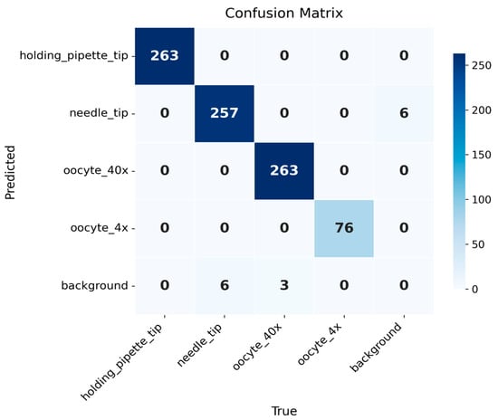
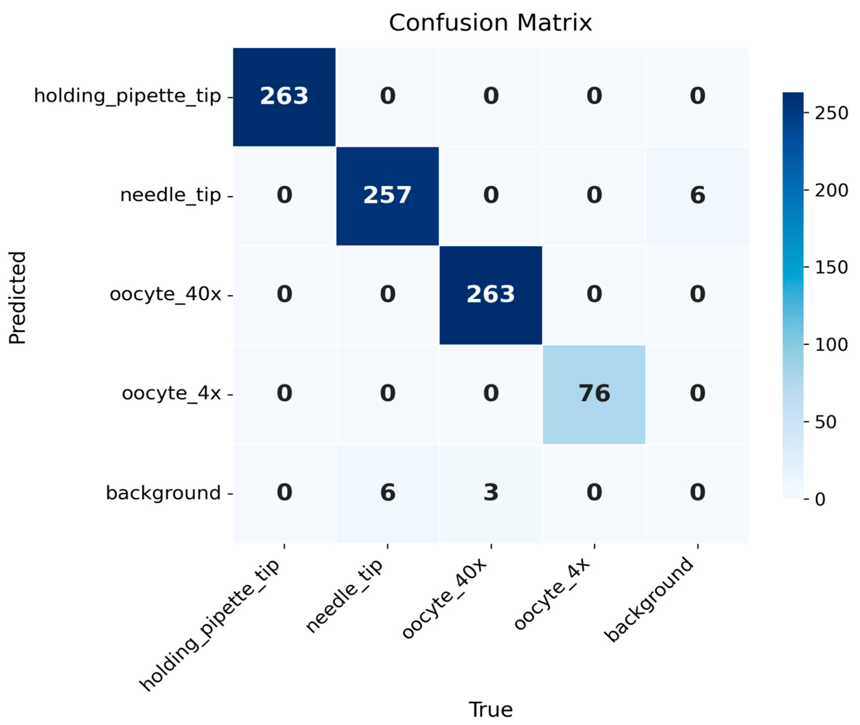
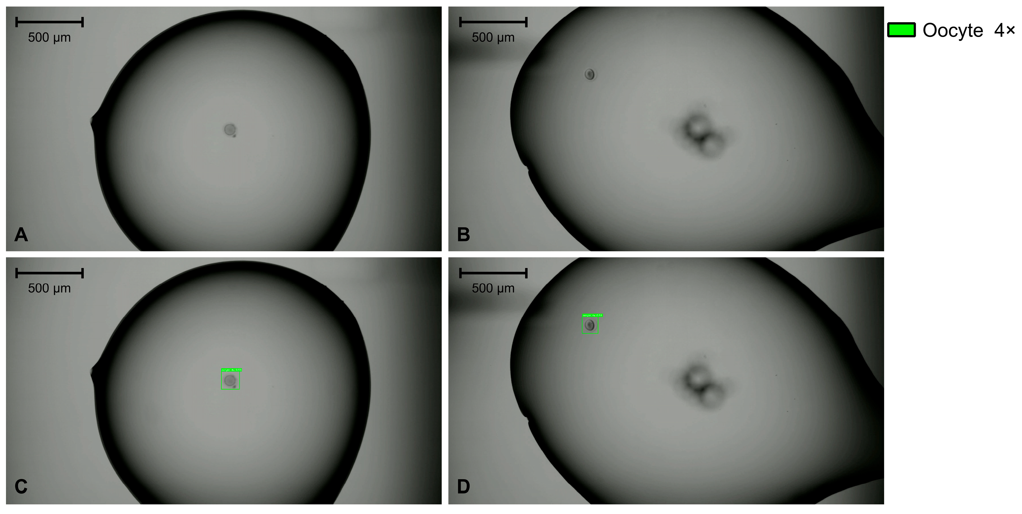
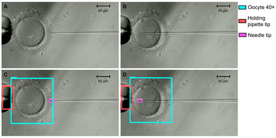
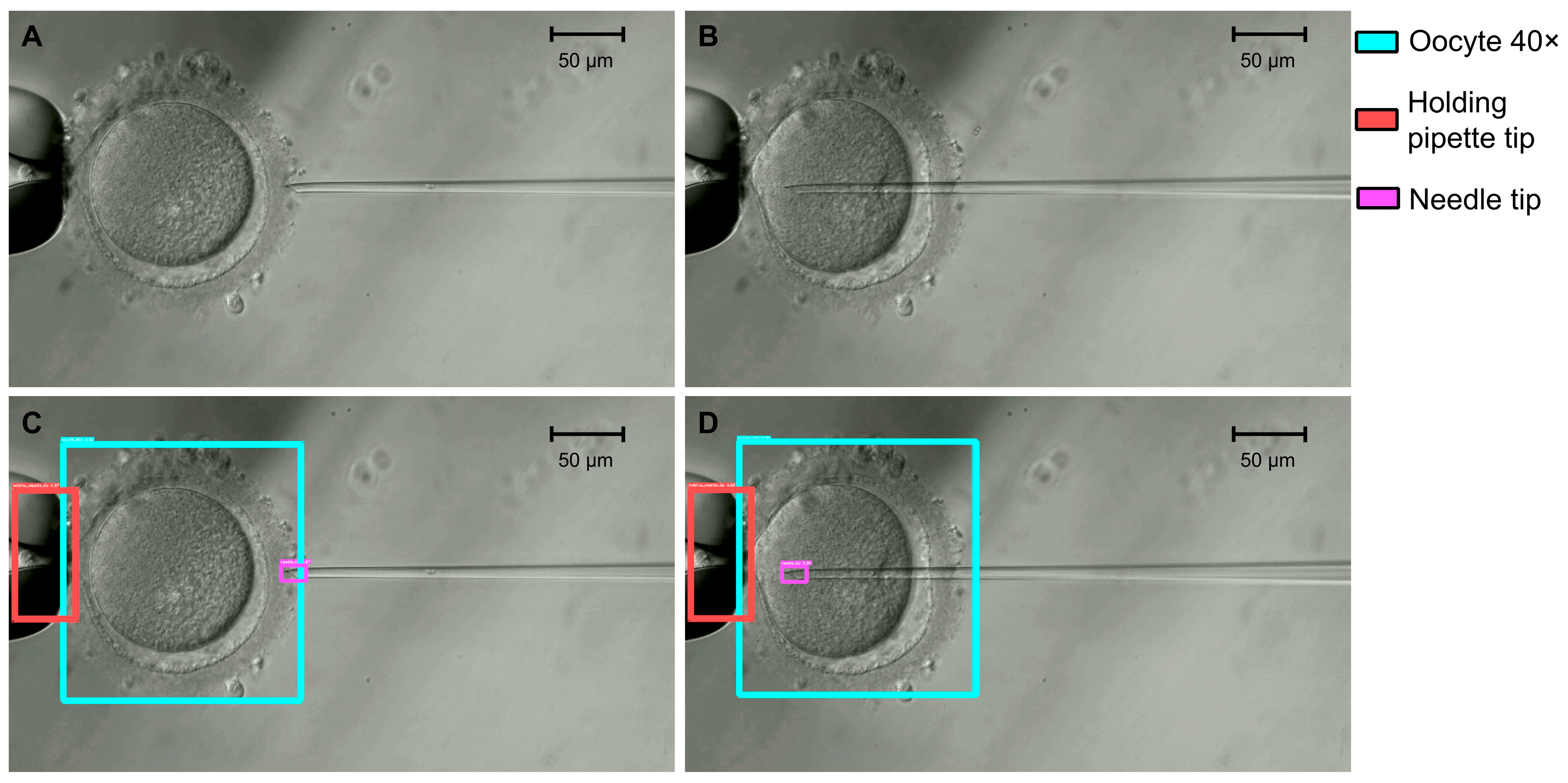
The T1 model localized the oocyte at two objective magnifications (4× and 40×), together with the holding-pipette and ICSI-needle tips at 40×, achieving a test mAP@0.50 of 0.988, mAP@0.75 of 0.910, and mAP@0.50:0.95 of 0.801. At a fixed confidence threshold of 0.25 (IoU matching threshold 0.5), macro-averaged precision, recall, and F1 were 0.994, 0.991, and 0.993 (Table 6 and Table 7). The holding-pipette tip and the oocyte at 4× were detected without errors (precision, recall, and F1 = 1.000), and the oocyte at 40× nearly so (F1 = 0.994). The needle tip was the most difficult class, with the lowest F1 (0.977) and the lowest AP@0.50:0.95 (0.621). The gap between its AP@0.50 (0.980) and AP@0.75 (0.688) indicates that the tip was reliably found but its box was less precisely placed at strict overlap thresholds, as expected for a small, thin, transparent structure. Figure 1 shows the confusion matrix for the selected model. Figure 2 and Figure 3 show examples at 4× and 40×, respectively.
Table 6.
Overall test metrics for the four-class detector (T1). Precision, recall, and F1 are macro-averages over the four classes, that is, the unweighted mean of the per-class values in Table 7, at a fixed confidence of 0.25 and an IoU matching threshold of 0.5. Values in parentheses are 95% CrIs.
Table 7.
Per-class test metrics for the four-class detector (T1). Counts and class-wise precision, recall, and F1 correspond to a fixed confidence of 0.25 and an IoU matching threshold of 0.5; the unweighted mean of these columns gives the macro-averaged values in Table 6.
Figure 1.
Confusion matrix of the T1 model. The model localizes four classes (holding pipette tip, needle tip, oocyte 40×, and oocyte 4×), with 263, 257, 263, and 76 true positives, respectively. Errors are confined to the needle tip class (6 false positives, 6 false negatives) and the oocyte 40× class (3 false negatives). Every false positive and false negative is a background confusion, with no inter-class misclassification.
Figure 2.
Examples of original images at 4× magnification (panels (A,B)) and the corresponding T1 detections for the oocyte 4× class (panels (C,D)). Scale bars, 500 μm.
Figure 3.
Examples of original images at 40× magnification (panels (A,B)) and the corresponding T1 detections for the oocyte 40×, needle tip, and holding pipette tip classes (panels (C,D)). Scale bars, 50 μm.
3.3. Sperm-in-Needle Detection (T2)
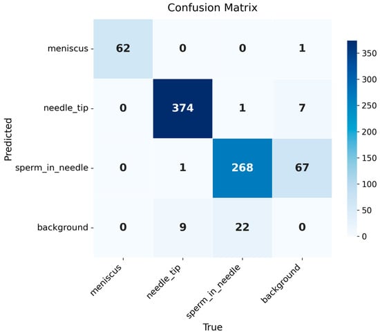
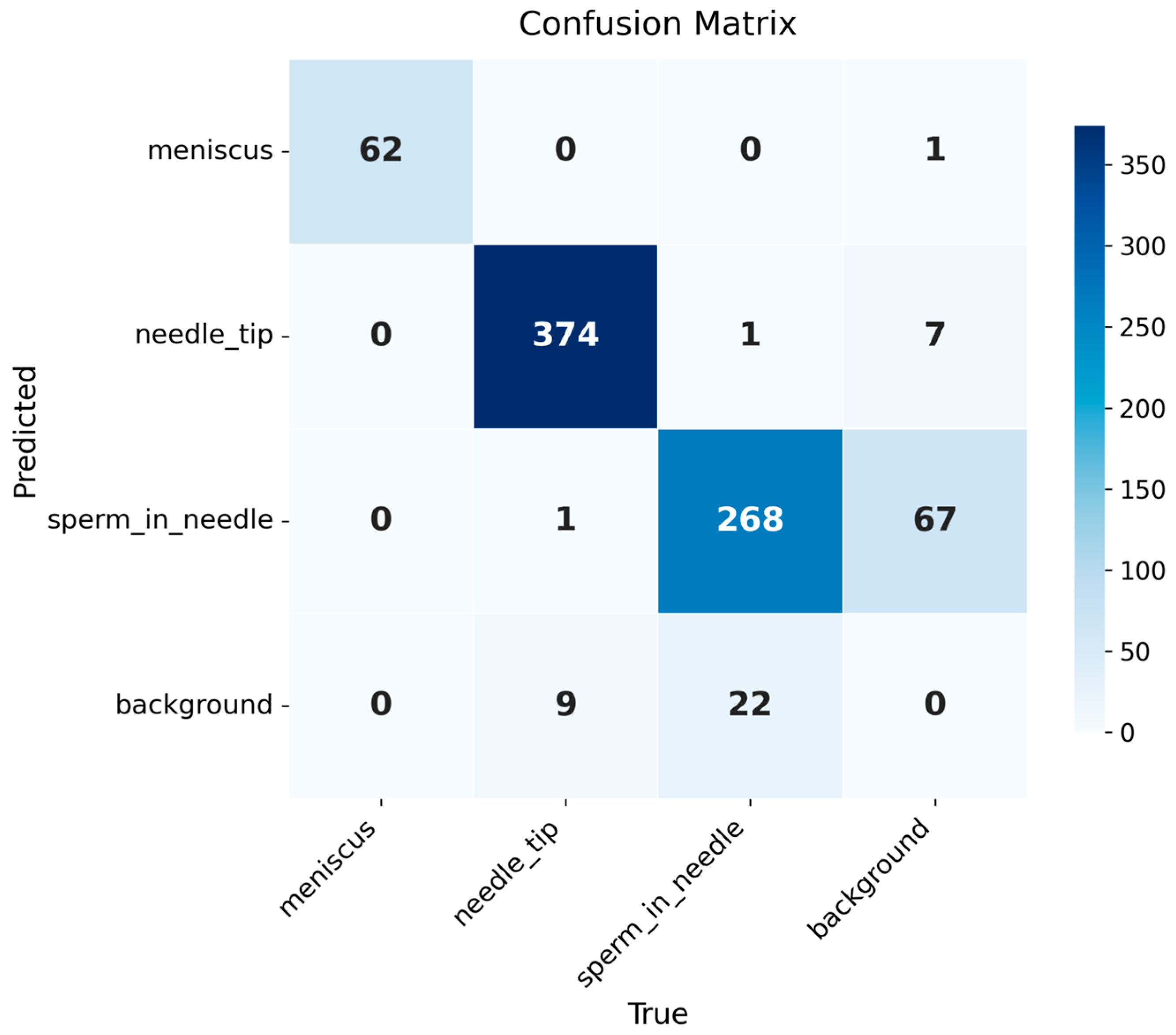
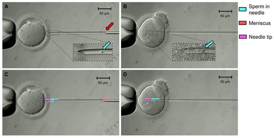
The T2 detector reached a test mAP@0.50 of 0.962, mAP@0.75 of 0.579, and mAP@0.50:0.95 of 0.573, with macro-averaged precision, recall, and F1 of 0.920, 0.965, and 0.941 (Table 8 and Table 9). The meniscus and the needle tip were detected with high accuracy (F1 = 0.992 and 0.977; AP@0.50 = 0.995 and 0.977). The sperm in needle class, the target intended to drive the visual-servoing controller, had the lowest precision (0.798; 95% CrI 0.752–0.838) and F1 (0.855; 95% CrI 0.823–0.882), with a recall of 0.921. Its errors were predominantly false positives (68, against 23 false negatives), indicating that the model detected sperm where none had been annotated more often than it missed a sperm that was present. Figure 4 shows the confusion matrix for model T2. The gap between AP@0.50 and AP@0.50:0.95 was largest for the meniscus (0.995 vs. 0.485), whose curved interface has no well-defined lateral extent, so the boundaries of its box are inherently ambiguous. Relevant examples are shown in Figure 5.
Table 8.
Overall test metrics for T2 (sperm-in-needle detector). Precision, recall, and F1 are macro-averages over the three classes, that is, the unweighted mean of the per-class values in Table 9, at a fixed confidence of 0.25 and an IoU matching threshold of 0.5. Values in parentheses are 95% CrIs.
Table 9.
Per-class test metrics for T2 (meniscus, needle tip, sperm-in-needle). Counts and class-wise precision, recall, and F1 correspond to a fixed confidence of 0.25 and an IoU matching threshold of 0.5; the unweighted mean of these columns gives the macro-averaged values in Table 8.
Figure 4.
Confusion matrix of the T2 model. The model distinguished the classes: meniscus, needle tip, and sperm in needle, with 62, 374, and 268 true positives, respectively. The sperm in needle class accounted for most of the errors (68 false positives, 23 false negatives), followed by the needle tip (8 false positives, 10 false negatives) and meniscus (1 false positive) classes. Most errors involved the background rather than another class.
Figure 5.
Examples of original images at 40× magnification (panels (A,B)) and the corresponding T2 detections (panels (C,D)). Insets show magnified views of the needle; arrows indicate the sperm (cyan) and the meniscus (red). Scale bars, 50 μm.
3.4. Sperm Head and Tail Segmentation (T3)
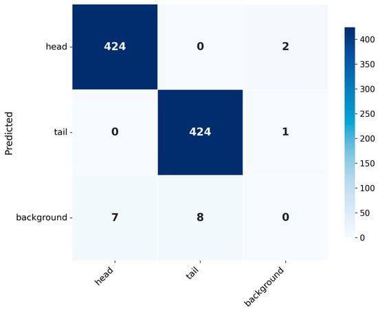
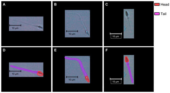
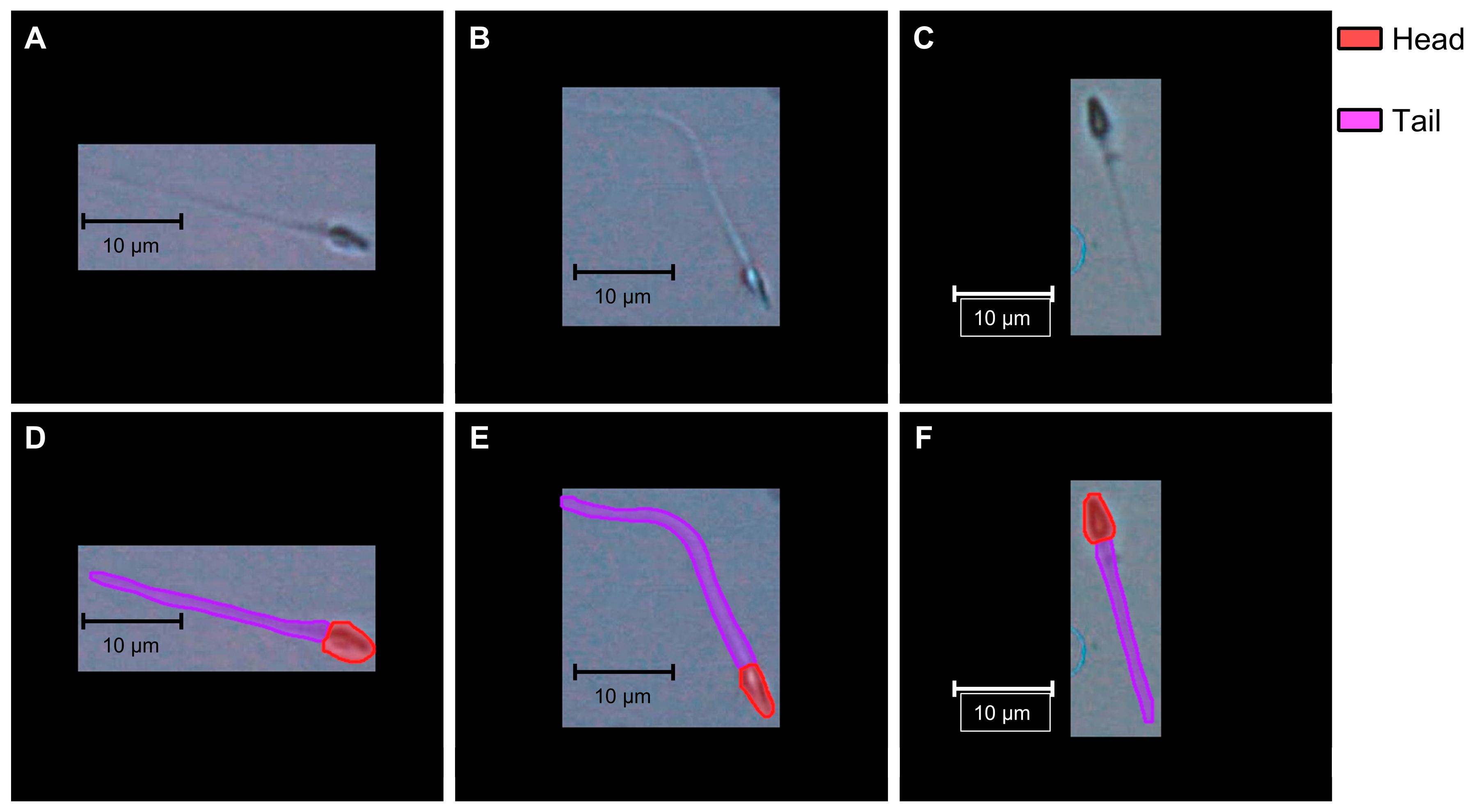
The T3 model reached a test mAP@0.50 of 0.985 and an mAP@0.50:0.95 of 0.850 for bounding boxes, and 0.990 and 0.725 for masks, with macro-averaged precision, recall, and F1 of 0.996, 0.983, and 0.990 for both outputs (Table 10 and Table 11). Sperm head and tail were segmented with similar precision and recall (F1 = 0.990 for both), but mask accuracy at strict overlap thresholds was lower for the tail (AP@0.50:0.95 = 0.680) than for the head (0.771), reflecting the difficulty of placing the boundaries of a thin, elongated structure. The corresponding box values were higher (0.862 for the head and 0.838 for the tail), confirming that coarse localization was more accurate than pixel-level mask placement. Figure 6 shows the confusion matrix for model T3, and Figure 7 shows examples of original sperm images at 40× magnification and the corresponding segmentation results.
Table 10.
Overall test metrics for T3, reported separately for bounding boxes and masks. Precision, recall, and F1 are macro-averages over the two classes, that is, the unweighted mean of the per-class values in Table 11, at a fixed confidence of 0.25 and an IoU matching threshold of 0.5. Values in parentheses are 95% CrIs.
Table 11.
Per-class test metrics for T3 (head and tail). Counts and class-wise precision, recall, and F1 correspond to a fixed confidence of 0.25 and an IoU matching threshold of 0.5; the unweighted mean of these columns gives the macro-averaged values in Table 10.
Figure 6.
Confusion matrix of the T3 model. The head and tail were each detected with 424 true positives. All errors were missed or spurious detections (head: 2 false positives, 7 false negatives; tail: 1 false positive, 8 false negatives), and no head was misclassified as a tail or vice versa. Box and mask outputs yielded identical counts, so the matrix applies to both.
Figure 7.
Examples of original sperm images at 40× magnification (panels (A–C)) and the corresponding T3 segmentation results (panels (D–F)). Scale bars, 10 μm.
3.5. Inference Latency
Per-image model inference latency is reported in Table 12; these values exclude image acquisition, data transfer, communication with the robotic controller, and control execution. Total latency was 11.58 ms for T1, 11.00 ms for T2, and 7.00 ms for T3, with low variability across repetitions (standard deviation ≤ 0.26 ms for every component). The forward pass accounted for most of the latency in all three models (88–96% of the total), whereas pre- and post-processing together took less than 1 ms. The two RT-DETR detectors, which processed 960 px × 960 px images, were slower than the segmentation model, which processed 320 px × 320 px images. In T3, post-processing took longer than pre-processing (0.65 vs. 0.20 ms) because it included NMS and mask decoding.
Table 12.
Per-image model inference latency on the test set (ms), measured on a single RTX 4090 GPU (FP32, batch size 1). Values exclude image acquisition, data transfer, communication with the robotic controller, and control execution.
4. Discussion
Unlike embryo assessment, where AI assists human decision-making, robotic ICSI requires AI to perceive a dynamic microscopic scene in real time and to guide physical manipulation. We asked whether off-the-shelf detection and segmentation architectures, fine-tuned on modest clinical datasets without architectural modification, could provide that perception. On the three ICSI tasks evaluated here, the selected models reached a test mAP@0.50 of 0.988 for oocyte and tool-tip detection (T1), 0.962 for sperm-in-needle detection (T2), and a mask mAP@0.50 of 0.990 for sperm head and tail segmentation (T3). These results suggest that publicly available models adapted by transfer learning with modest clinical datasets are a feasible starting point for automating the visual tasks of ICSI, although validation on other microscopes and clinical sites is still needed.
In practice, the three models are meant to operate one after another, each during a specific stage of the ICSI procedure:
- Sperm immobilization and aspiration (40×). T3 segments the head and tail of the selected spermatozoon in a polyvinylpyrrolidone (PVP) droplet; the head position and the course of the tail are used to position the needle for immobilization and tail-first aspiration.
- Sperm positioning in the needle (40×). After aspiration, T2 detects the needle tip, the meniscus, and the sperm, providing the measurements intended for the controller that regulates the sperm’s position in the needle.
- Oocyte localization (4×). T1 locates the oocytes in the injection dish.
- Oocyte holding and injection (40×). T1 localizes the oocyte and the tool tips for alignment; T2 then monitors the sperm in the needle during penetration and injection, until it is deposited in the cytoplasm.
Transitions between stages are triggered by operator confirmation. Because only one model runs at a time, the inference latency of each stage is determined by a single model.
All three models processed an image in 7.0–11.6 ms on a single RTX 4090 GPU, shorter than the camera frame period (66.7 ms at 15 frames per second). This shows that model inference is computationally compatible with processing every frame, but it does not establish real-time closed-loop performance: the latency of the complete robotic system, which adds image acquisition, data transfer, communication with the controller, and control execution, was not measured. This distinction is most relevant for T2, whose detections are intended to drive a visual-servoing controller.
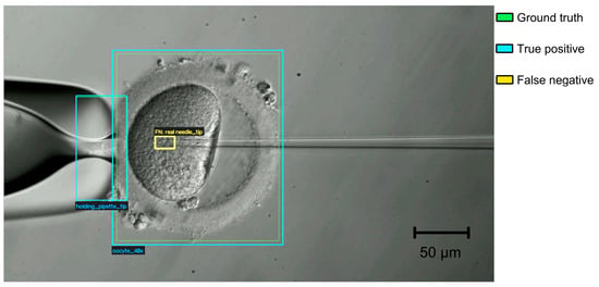
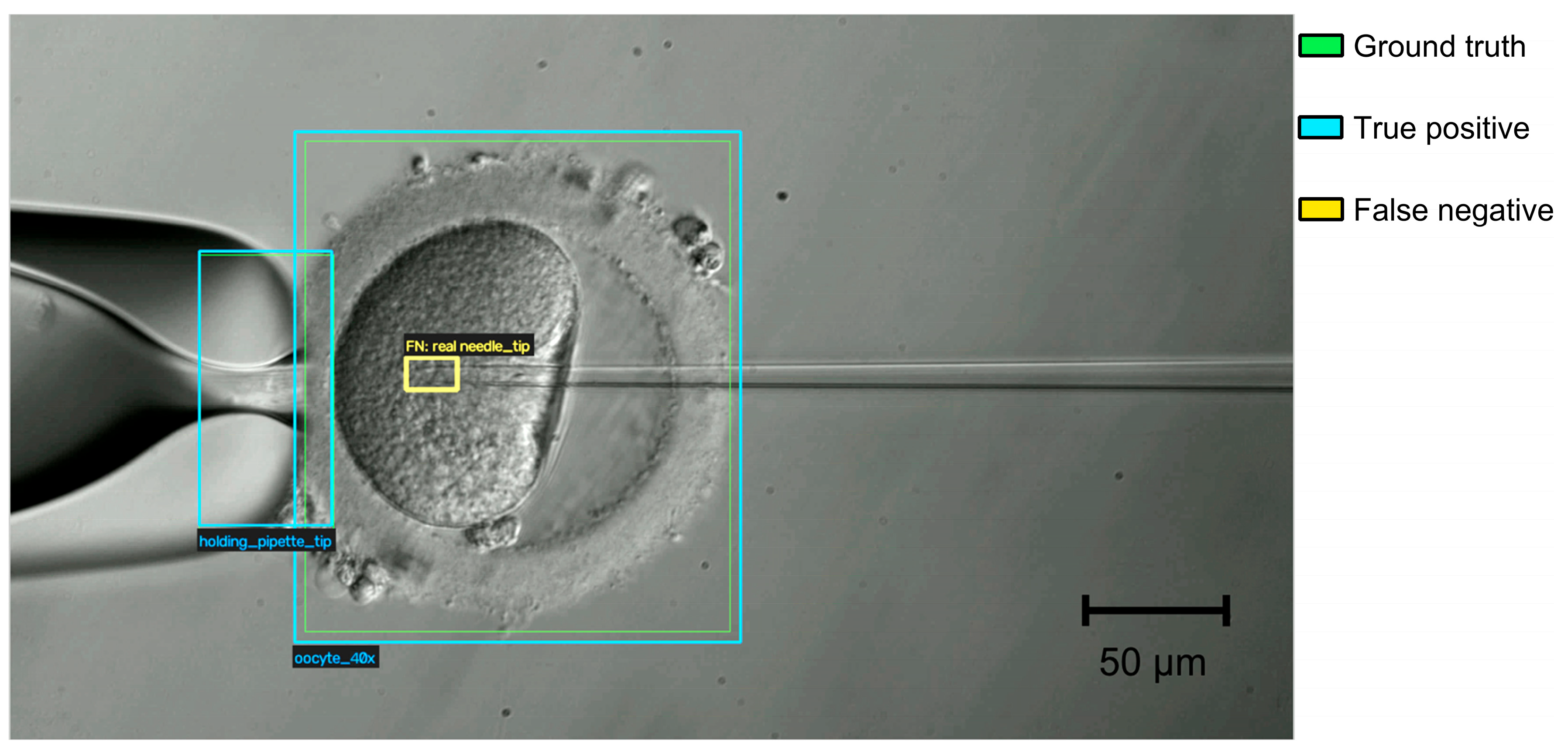
With the selected T1 model, errors in the test set were limited to two classes: needle tip (6 false positives and 6 false negatives; precision = recall = 0.977) and oocyte 40× (3 false negatives). The confusion matrix (Figure 1) shows that all errors were confusions with the background, with none between classes. The needle tip also had the lowest AP@0.75 (0.688) and AP@0.50:0.95 (0.621) among the T1 classes. At the 960 px × 960 px input resolution, one pixel corresponds to approximately 0.48 μm at 40× (Section 2.3), so the lumen of the needle tip (inner diameter approximately 5 μm) spans only about 10 input pixels, and small errors in box placement may substantially reduce IoU at strict thresholds. Missed tips typically occurred after the needle had penetrated the oocyte (Figure 8). There, the thin glass tip must be distinguished from the granular, heterogeneous texture of the ooplasm (the same difficulty described below for the sperm inside the needle in T2), and the tip may lie slightly outside the focal plane, which further reduces its contrast. Because the needle is a rigid tool moved by a motorized micromanipulator, its tip position could be estimated from the last detection and the commanded displacement of the manipulator, or by tracking the tip across frames, so that isolated errors in single frames would not interrupt the procedure.
Figure 8.
Example of a false-negative detection by model T1 at 40× magnification. The oocyte and the holding pipette tip are correctly detected (blue boxes; the ground-truth boxes, in green, coincide with them), whereas the tip of the injection needle inside the ooplasm is not detected (yellow box, ground-truth position). Scale bar, 50 μm.
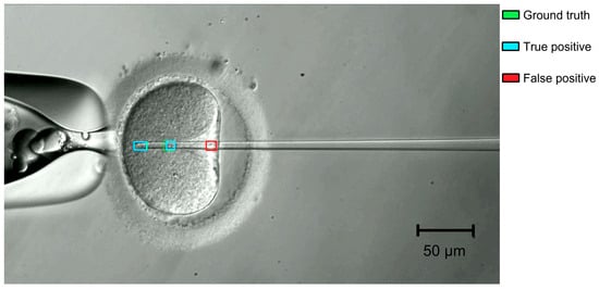
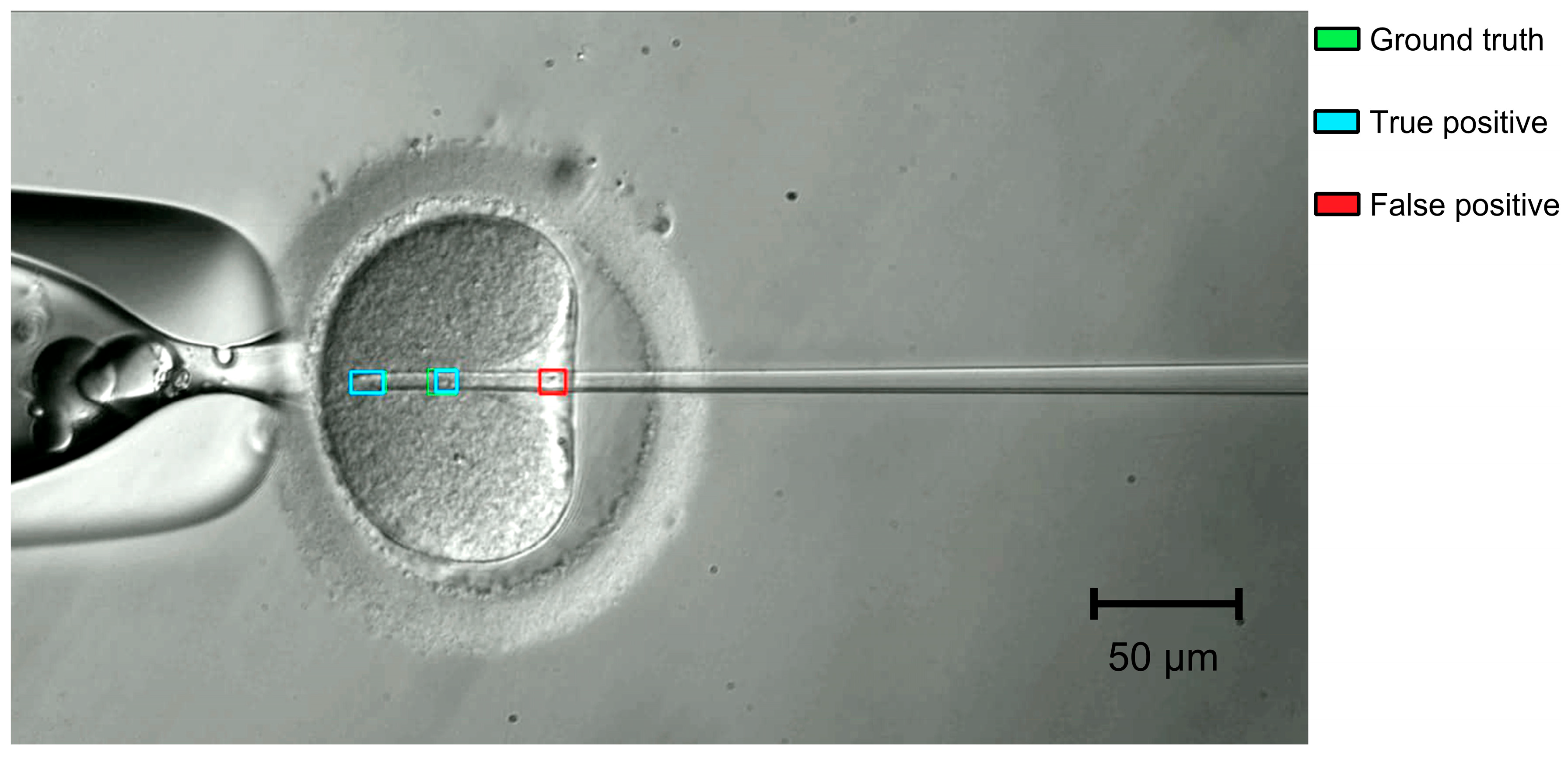
The sperm in needle class had the lowest precision (0.798) and F1 (0.855) among the T2 classes. Its errors were mainly false positives (68, against 23 false negatives). Almost all of them (67 of 68) involved the background rather than another class (needle tip or meniscus), so the detector reported a sperm where none was present rather than mistaking one class for another. Two conditions caused most of these errors. First, as with T1, once the needle penetrates the oocyte the sperm must be distinguished from the granular cytoplasm, where organelles, lipid droplets, and other structures produce local intensity variations that can resemble the sperm’s shape. Second, small droplets of the oil covering the medium in the injection dish can stick to the needle. Their rounded, high-contrast outlines can resemble a sperm inside the needle and be detected as one (Figure 9). The difficulty is compounded by the fact that T2 processes each frame independently and does not exploit the temporal continuity of the sperm’s position. Coupling the detector with a tracking algorithm (e.g., a Kalman filter that predicts and propagates the sperm’s position across frames) could help maintain a consistent track through transient ambiguities, suppress spurious single-frame detections, and provide temporally stable estimates for the intended visual-servoing controller, including during the intracytoplasmic phase. Persistent artifacts, such as an oil droplet that stays on the needle, would not be removed by tracking alone and should be better represented in the training data. Combining per-frame detection with frame-to-frame tracking is therefore a natural next step toward reliable sperm localization throughout the injection sequence.
Figure 9.
Example of a false-positive detection by model T2 at 40× magnification. A small oil droplet stuck to the injection needle is detected as sperm in needle (red box), although no sperm is present at that location. Green and cyan boxes indicate the ground truth and true-positive detections, respectively. Scale bar, 50 μm.
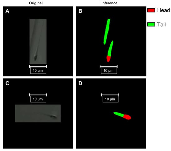
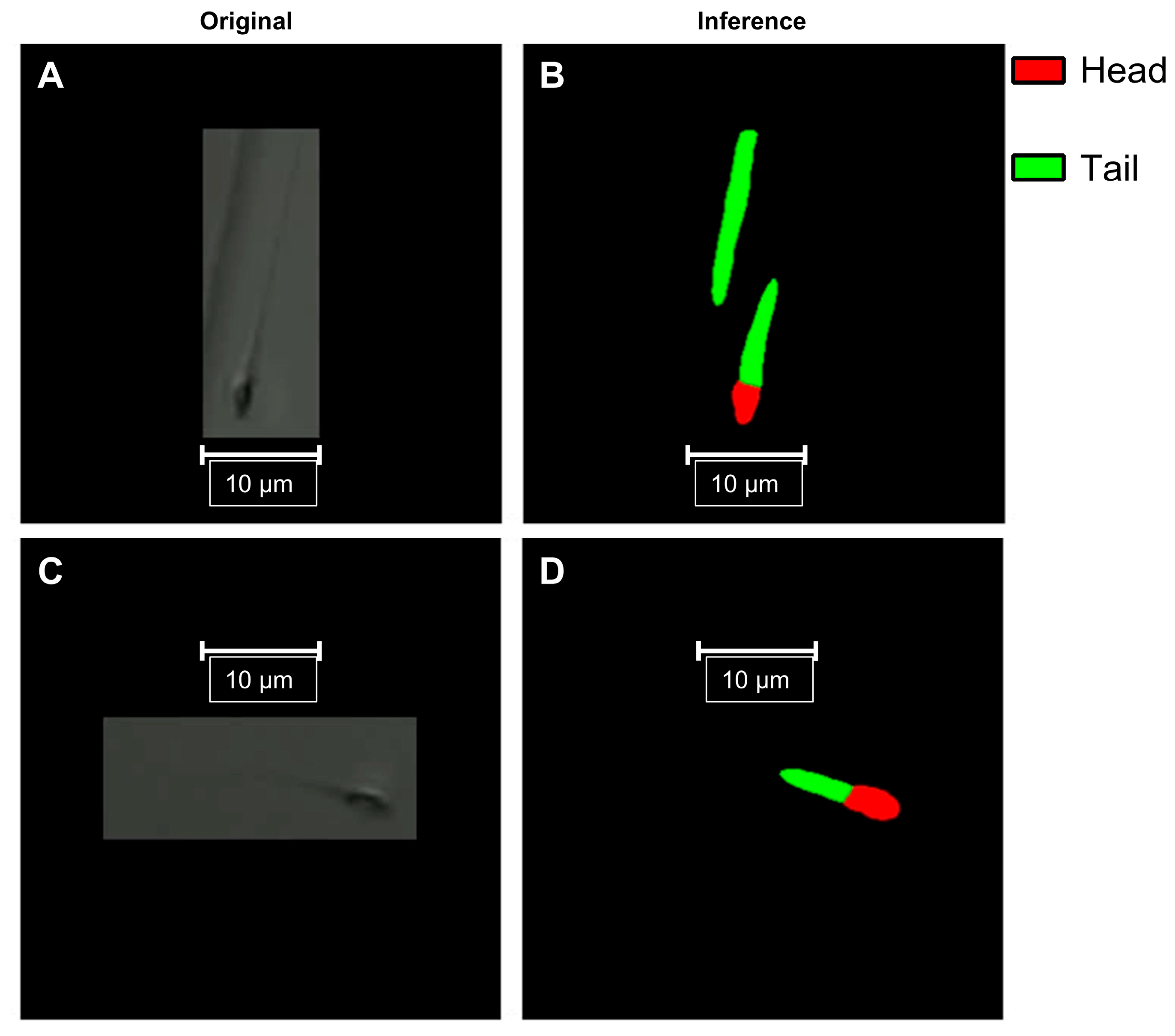
For T3, the mask mAP@0.50:0.95 was 0.725, compared with 0.850 for bounding boxes, reflecting imaging challenges specific to the sperm tail. First, the human flagellum is extremely thin (approximately 0.88 μm in diameter at the midpiece, tapering to approximately 0.17 μm at the terminal filament) [30], so at 40× the tail spans only a few pixels and its boundary is highly sensitive to sub-pixel localization errors. Second, sperm are immobilized in a PVP droplet several tens of micrometers high, whereas the depth of field of a 40× objective is only 1–2 μm; tails lying away from the focal plane therefore appear blurred or partly invisible, which makes their boundaries ambiguous. Figure 10 shows representative errors: in the upper row, part of the edge of the PVP droplet, which appears as a thin, elongated line similar to a flagellum, was segmented as an additional tail without an associated head; in the lower row, the tail mask was truncated and did not cover the faint distal part of the flagellum, as expected for a tail partly outside the focal plane. These errors mainly affect the extent and boundaries of the tail rather than the position of the head or the orientation of the proximal tail, which are the features needed to position the needle. Unlike an axis-aligned bounding box, the mask provides this orientation, and given the positioning accuracy of about 2 μm required by our system, mask mAP@0.50 (0.990) is a more relevant indicator for this purpose than mask mAP@0.50:0.95. False positives such as the droplet edge could be removed with simple post-processing rules, for example by discarding tail instances that are not connected to a head, since each spermatozoon has a single head and a single tail.
Figure 10.
Examples of T3 segmentation errors in images acquired with the 40× objective. Panels (A,C) (left column): original images; panels (B,D) (right column): predicted masks (red, head; green, tail). Panels (A,B) (upper row): part of the edge of the PVP droplet is segmented as an additional tail without an associated head. Panels (C,D) (lower row): the tail mask is truncated and does not include the faint distal part of the flagellum. Scale bars, 10 μm.
The present evaluation focused on detection and segmentation performance. Assessing the models’ effect on downstream clinical outcomes, together with prospective and human-in-the-loop studies and an analysis of inter-annotator agreement, will be the subject of future work. Although each model was trained independently, together they represent key components of a unified perception system for robotic ICSI. Future work will integrate these modules into a single closed-loop platform capable of autonomously executing clinically relevant micromanipulation tasks, with the aim of making IVF laboratory procedures more standardized and reproducible.
Beyond unmodified architectures, several strategies have been proposed to improve deep learning for medical images, including deep ensembles, attention-based convolutional networks, vision transformers, explainability methods, and task-specific modifications of YOLO, such as lightweight attention modules for detecting cells in microscopy images [31]. Here, we deliberately elected to use unmodified, publicly available architectures to establish a reproducible baseline against which such modifications can be measured. Some of these ideas are already represented among the models compared here: RT-DETR, selected for T1 and T2, uses a transformer encoder–decoder, and YOLO12 incorporates area attention in its backbone. Others must be weighed against the latency budget of robotic ICSI; an ensemble of k models, for example, multiplies inference time roughly k-fold. Explainability is less pressing here than for image-level classifiers, because the outputs (bounding boxes and masks overlaid on each frame) can be inspected directly by the operator. With this baseline in place, lightweight attention modules, transformer backbones for embedded deployment, and a systematic, quantitative analysis of failure modes are natural next steps.
Limitations
All data were acquired at a single clinical center on one custom-built inverted microscope, with a single camera and relief-contrast illumination from a red LED. We did not evaluate performance with other microscopes, optics, illumination sources, or culture media, and domain shift from any of these may reduce accuracy, so the models need external validation before they are used in other settings. The cohort is also small: 50, 46, and 41 patients contributed data to T1, T2, and T3, respectively. Although the data were partitioned at the patient level, the credible intervals reported here describe instance-level uncertainty, that is, how precisely each metric is estimated from the instances in the test set. Because these intervals assume independent instances, whereas frames from the same patient’s videos are correlated, they likely understate this uncertainty. Furthermore, the intervals do not describe patient-level generalizability, that is, how performance would vary across new patients. With only seven or eight patients per test set, between-patient variability could not be estimated reliably; the results should therefore be read as evidence of feasibility rather than as precise estimates of performance in the wider patient population. Each model was trained once on a single partition, credible intervals are reported only for precision, recall, and F1, and differences between candidate architectures were not tested statistically; performance could differ under alternative partitions or random seeds. Each image was annotated by one annotator and reviewed by a senior embryologist, and inter-annotator agreement was not assessed, so we could not quantify the reliability of the reference labels; this matters most for the sperm tail, whose boundaries are ambiguous outside the focal plane. A systematic ablation of the pre-processing and augmentation steps was not performed beyond the variants compared in Table 3. The evaluation covers only offline detection and segmentation: closed-loop robotic experiments, end-to-end latency, control accuracy, and comparison with embryologists were outside the scope of this study, and system-level experiments are still needed to show whether the models’ outputs are accurate and stable enough to drive closed-loop robotic control. Finally, this is an internal validation performed at a single company (Conceivable Life Sciences). The dataset and the platform belong to the developers of the system, who also trained, selected, and evaluated the models; independent replication is therefore needed.
5. Conclusions
We evaluated off-the-shelf deep learning models, fine-tuned by transfer learning, on three computer vision tasks of the ICSI micromanipulation stage: oocyte and tool-tip detection (T1), sperm-in-needle detection (T2), and sperm head-and-tail segmentation (T3). With datasets acquired during clinical procedures and partitioned at the patient level, all three models reached high accuracy on patients not seen during training, with model inference latencies of 7.0–11.6 ms per image on a single GPU, short enough to process every camera frame. These results come from a single center, a single custom microscope, and a single training run per task, and should be regarded as a proof of concept. They suggest that off-the-shelf models are a feasible basis for the perception layer of robotic ICSI. Whether the models’ outputs are accurate and stable enough for closed-loop robotic control, whether the complete robotic system, including image acquisition, communication, and control execution, meets the latency required for closed-loop operation, and whether the models generalize to other microscopes, sites, and patient cohorts, remain to be established in system-level and multi-site studies.
Supplementary Materials
The following supporting information can be downloaded at: https://www.mdpi.com/article/10.3390/bioengineering13111397/s1, Table S1: Per-class precision, recall, and F1 with 95% credible intervals for the selected models.
Author Contributions
M.R.-L.: methodology, software, validation. A.C.-B.: conceptualization, methodology, supervision, writing—review and editing. V.O.-H.: methodology, software, validation. C.M.-Z.: methodology, software, validation. D.M.-Z.: methodology, validation. G.S.: writing—review and editing. J.C.: conceptualization, methodology, supervision, writing—review and editing. G.M.-R.: conceptualization, data curation, investigation, methodology, supervision, validation, writing—original draft preparation, writing—review and editing. All authors have read and agreed to the published version of the manuscript.
Funding
This research did not receive any specific grant from funding agencies in the public, commercial or not-for-profit sectors.
Institutional Review Board Statement
This study received institutional review board (IRB) approval (reference RA-2024-01, granted 12 August 2024) from the Comité de Ética en Investigación of New Hope Fertility Center, which is registered with the Mexican national bioethics commission as CONBIOÉTICA-09-CEI-001-20170131, and was registered at ClinicalTrials.gov under identifier NCT06581068.
Informed Consent Statement
Informed consent was obtained from all subjects involved in the study.
Data Availability Statement
The annotated datasets were constructed for this study from clinical microscopy images acquired during routine IVF procedures. They are not publicly available due to institutional data governance policies; the datasets are the property of Conceivable Life Sciences and are subject to data use restrictions.
Acknowledgments
The authors wish to thank the embryology team at Hope IVF Fertility Clinic (Mexico City, Mexico) for their support in data collection. We also thank the embryology team at Conceivable Life Sciences for annotating the data. During the preparation of this work, the authors used Claude Opus (v5.5 Anthropic)to assist with copyediting. After using this tool/service, the authors reviewed and edited the content as needed and take full responsibility for the content of the published article.
Conflicts of Interest
Mario Reyes-Llamas: employee, stockholder (Conceivable Life Sciences); Alejandro Chávez-Badiola: company officer, stockholder, patent inventor (Conceivable Life Sciences); stockholder (IVF 20.0); Vladimir Ocegueda-Hernández: employee, stockholder, patent inventor (Conceivable Life Sciences); Celina Méndez-Zavala: employee, stockholder (Conceivable Life Sciences); Diana Mancera-Zapata: employee, stockholder (Conceivable Life Sciences); Giuseppe Silvestri: employee, stockholder (Conceivable Life Sciences); Jacques Cohen: company officer, stockholder, patent inventor (Conceivable Life Sciences); stockholder (IVF 20.0); Gerardo Mendizabal-Ruiz: paid consultant, stockholder, patent inventor (Conceivable Life Sciences).
Abbreviations
The following abbreviations are used in this manuscript:
| AI | Artificial Intelligence |
| AMP | Automatic Mixed Precision |
| AP | Average Precision |
| CLAHE | Contrast-Limited Adaptive Histogram Equalization |
| CrI | Credible Interval |
| DETR | Detection Transformer |
| FP32 | 32-bit Floating Point |
| GPU | Graphics Processing Unit |
| ICSI | Intracytoplasmic Sperm Injection |
| IoU | Intersection over Union |
| IVF | In Vitro Fertilization |
| LCD | Liquid-Crystal Display |
| LED | Light-Emitting Diode |
| mAP | Mean Average Precision |
| NMS | Non-Maximum Suppression |
| PVP | Polyvinylpyrrolidone |
| RC | Relief Contrast |
| RT-DETR | Real-Time Detection Transformer |
| YOLO | You Only Look Once |
References
- The ESHRE Guideline Group on Female Fertility Preservation; Anderson, R.A.; Amant, F.; Braat, D.; D’Angelo, A.; Chuva de Sousa Lopes, S.M.; Demeestere, I.; Dwek, S.; Frith, L.; Lambertini, M.; et al. ESHRE guideline: Female fertility preservation. Hum. Reprod. Open 2020, 2020, hoaa052. [Google Scholar] [CrossRef] [PubMed]
- Practice Committee and Genetic Counseling Professional Group of the American Society for Reproductive Medicine. Indications and management of preimplantation genetic testing for monogenic conditions: A committee opinion. Fertil. Steril. 2023, 120, 61–71. [Google Scholar] [CrossRef] [Scilit] [PubMed]
- Ethics Committee of the American Society for Reproductive Medicine. Access to fertility services by transgender and nonbinary persons: An Ethics Committee opinion. Fertil. Steril. 2021, 115, 874–878. [Google Scholar] [CrossRef] [Scilit] [PubMed]
- Wang, R.; Au, L.S.; Wei, D.; Legro, R.S.; Wang, Z.; Sun, Y.; Wu, K.; Vuong, L.N.; Hardy, P.; Pinborg, A.B.; et al. Who benefits most from a freeze-all embryo transfer strategy? An individual participant data meta-analysis of randomised controlled trials (INFORM). Fertil. Steril. 2024, 122, e66. [Google Scholar] [CrossRef] [Scilit]
- Lorimer, J.; McLachlan, R.; Zander-Fox, D.; O’Bryan, M.K.; Nosrati, R. AI and automation in assisted reproduction. Nat. Rev. Bioeng. 2026, 4, 818–839. [Google Scholar] [CrossRef] [Scilit]
- Tiegs, A.W.; Scott, R.T. Evaluation of fertilization, usable blastocyst development and sustained implantation rates according to intracytoplasmic sperm injection operator experience. Reprod. Biomed. Online 2020, 41, 19–27. [Google Scholar] [CrossRef] [Scilit] [PubMed]
- Alikani, M.; Campbell, A. Shaping the future of the IVF laboratory: Standardization for more predictable outcomes. Reprod. Biomed. Online 2025, 50, 104854. [Google Scholar] [CrossRef] [Scilit] [PubMed]
- Bendus, A.E.B.; Mayer, J.F.; Shipley, S.K.; Catherino, W.H. Interobserver and intraobserver variation in day 3 embryo grading. Fertil. Steril. 2006, 86, 1608–1615. [Google Scholar] [CrossRef] [Scilit] [PubMed]
- Storr, A.; Venetis, C.A.; Cooke, S.; Kilani, S.; Ledger, W. Inter-observer and intra-observer agreement between embryologists during selection of a single Day 5 embryo for transfer: A multicenter study. Hum. Reprod. 2017, 32, 307–314. [Google Scholar] [CrossRef] [Scilit] [PubMed]
- Paternot, G.; Wetzels, A.M.; Thonon, F.; Vansteenbrugge, A.; Willemen, D.; Devroe, J.; Debrock, S.; D’Hooghe, T.M.; Spiessens, C. Intra-and interobserver analysis in the morphological assessment of early stage embryos during an IVF procedure: A multicentre study. Reprod. Biol. Endocrinol. 2011, 9, 127. [Google Scholar] [CrossRef] [Scilit] [PubMed]
- Manna, C.; Nanni, L.; Lumini, A.; Pappalardo, S. Artificial intelligence techniques for embryo and oocyte classification. Reprod. Biomed. Online 2013, 26, 42–49. [Google Scholar] [CrossRef] [Scilit] [PubMed]
- Zaninovic, N.; Rosenwaks, Z. Artificial intelligence in human in vitro fertilization and embryology. Fertil. Steril. 2020, 114, 914–920. [Google Scholar] [CrossRef] [Scilit] [PubMed]
- Louis, C.M.; Erwin, A.; Handayani, N.; Polim, A.A.; Boediono, A.; Sini, I. Review of computer vision application in in vitro fertilization: The application of deep learning-based computer vision technology in the world of IVF. J. Assist. Reprod. Genet. 2021, 38, 1627–1639. [Google Scholar] [CrossRef] [Scilit] [PubMed]
- Mendizabal-Ruiz, G.; Paredes, O.; Alvarez, A.; Acosta-Gómez, F.; Hernandez-Morales, E.; González-Sandoval, J.; Mendez-Zavala, C.; Borrayo, E.; Chavez-Badiola, A. Artificial intelligence in human reproduction. Arch. Med. Res. 2024, 55, 103131. [Google Scholar] [CrossRef] [Scilit] [PubMed]
- Lu, Z.; Zhang, X.; Leung, C.; Esfandiari, N.; Casper, R.F.; Sun, Y. Robotic ICSI (intracytoplasmic sperm injection). IEEE Trans. Biomed. Eng. 2011, 58, 2102–2108. [Google Scholar] [CrossRef] [Scilit] [PubMed]
- Zhang, Z.; Dai, C.; Huang, J.; Wang, X.; Liu, J.; Ru, C.; Pu, H.; Xie, S.; Zhang, J.; Moskovtsev, S.; et al. Robotic immobilization of motile sperm for clinical intracytoplasmic sperm injection. IEEE Trans. Biomed. Eng. 2019, 66, 444–452. [Google Scholar] [CrossRef] [Scilit] [PubMed]
- Costa-Borges, N.; Munne, S.; Albo, E.; Mas, S.; Castello, C.; Giralt, G.; Lu, Z.; Chau, C.; Acacio, M.; Mestres, E.; et al. First babies conceived with automated intracytoplasmic sperm injection. Reprod. Biomed. Online 2023, 47, 103237. [Google Scholar] [CrossRef] [Scilit] [PubMed]
- Jiang, V.S.; Kartik, D.; Thirumalaraju, P.; Kandula, H.; Kanakasabapathy, M.K.; Souter, I.; Dimitriadis, I.; Bormann, C.L.; Shafiee, H. Advancements in the future of automating micromanipulation techniques in the IVF laboratory using deep convolutional neural networks. J. Assist. Reprod. Genet. 2023, 40, 251–257. [Google Scholar] [CrossRef] [Scilit] [PubMed]
- Mohamed, M.; Yuriko, E.; Kawagoe, Y.; Kawamura, K.; Ikeuchi, M. AI-based augmented reality microscope for real-time sperm detection and tracking in micro-TESE. Bioengineering 2026, 13, 102. [Google Scholar] [CrossRef] [Scilit] [PubMed]
- Mendizabal-Ruiz, G.; Chavez-Badiola, A.; Hernández-Morales, E.; Valencia-Murillo, R.; Ocegueda-Hernández, V.; Costa-Borges, N.; Mestres, E.; Acacio, M.; Matia-Algué, Q.; Farías, A.F.S.; et al. A digitally controlled, remotely operated ICSI system: Case report of the first live birth. Reprod. Biomed. Online 2025, 50, 104943. [Google Scholar] [CrossRef] [Scilit] [PubMed]
- Chavez-Badiola, A.; Mendizabal-Ruiz, G.; Flores-Saiffe Farías, A.; Costa-Borges, N.; Murray, A.; Alikani, M.; Silvestri, G.; Millan, C.; Hernández-Morales, E.; Valencia-Murillo, R.; et al. Automated oocyte retrieval, denudation, sperm preparation, and ICSI in the IVF laboratory: A proof-of-concept study and report of the first live births. Hum. Reprod. 2026, 41, 214–230. [Google Scholar] [CrossRef] [Scilit] [PubMed]
- Chavez-Badiola, A.; Valadez Aguilar, A.; Mendizabal-Ruiz, G.; Flores-Saiffe Farías, A.; Hernández-Morales, E.; Álvarez Lopez, A.; Sánchez-González, D.J.; Costa-Borges, N.; Murray, A.; Alikani, M.; et al. Automation of sperm preparation, oocyte retrieval and denudation, ICSI, and vitrification in IVF: Insights from a proof-of-concept study. Hum. Reprod. 2026, in press. [Google Scholar] [CrossRef] [Scilit] [PubMed]
- Redmon, J.; Divvala, S.; Girshick, R.; Farhadi, A. You only look once: Unified, real-time object detection. In Proceedings of the IEEE Conference on Computer Vision and Pattern Recognition (CVPR), Las Vegas, NV, USA, 27–30 June 2016; pp. 779–788. [Google Scholar] [CrossRef] [Scilit]
- Zhao, Y.; Lv, W.; Xu, S.; Wei, J.; Wang, G.; Dang, Q.; Liu, Y.; Chen, J. DETRs beat YOLOs on real-time object detection. In Proceedings of the IEEE/CVF Conference on Computer Vision and Pattern Recognition (CVPR), Seattle, WA, USA, 17–21 June 2024; pp. 16965–16974. [Google Scholar] [CrossRef] [Scilit]
- Carion, N.; Massa, F.; Synnaeve, G.; Usunier, N.; Kirillov, A.; Zagoruyko, S. End-to-end object detection with transformers. In European Conference on Computer Vision (ECCV); Springer: Cham, Switzerland, 2020; pp. 213–229. [Google Scholar] [CrossRef] [Scilit]
- He, K.; Gkioxari, G.; Dollár, P.; Girshick, R. Mask R-CNN. In Proceedings of the IEEE International Conference on Computer Vision (ICCV), Venice, Italy, 22–29 October 2017; pp. 2961–2969. [Google Scholar] [CrossRef] [Scilit]
- Sapkota, R.; Karkee, M. Ultralytics YOLO evolution: An overview of YOLO26, YOLO11, YOLOv8, and YOLOv5 object detectors for computer vision and pattern recognition. arXiv 2025, arXiv:2510.09653. [Google Scholar] [CrossRef] [Scilit]
- Tian, Y.; Ye, Q.; Doermann, D. YOLOv12: Attention-centric real-time object detectors. Adv. Neural Inf. Process. Syst. 2026, 38, 78433–78457. [Google Scholar] [CrossRef] [Scilit]
- Jocher, G.; Qiu, J.; Liu, M.; Lyu, S.; Akyon, F.C.; Kalfaoglu, M.E. Ultralytics YOLO26: Unified Real-Time End-to-End Vision Models. arXiv 2026, arXiv:2606.03748. [Google Scholar] [CrossRef] [Scilit]
- Serres, C.; Escalier, D.; David, G. Ultrastructural morphometry of the human sperm flagellum with a stereological analysis of the lengths of the dense fibres. Biol. Cell 1984, 49, 153–161. [Google Scholar] [CrossRef] [Scilit] [PubMed]
- Yurdakul, M.; Taşdemir, Ş. BC-YOLO: MBConv-ECA based YOLO framework for blood cell detection. Signal Image Video Process. 2025, 19, 712. [Google Scholar] [CrossRef] [Scilit]

Disclaimer/Publisher’s Note: The statements, opinions and data contained in all publications are solely those of the individual author(s) and contributor(s) and not of MDPI and/or the editor(s). MDPI and/or the editor(s) disclaim responsibility for any injury to people or property resulting from any ideas, methods, instructions or products referred to in the content. |
© 2026 by the authors. Licensee MDPI, Basel, Switzerland. This article is an open access article distributed under the terms and conditions of the Creative Commons Attribution (CC BY) license.