


Highlights
What are the main findings?
- The audited decoder achieved 80.70% mean window balanced accuracy across 23 nominal test units.
- Without target-data alignment, balanced accuracy fell by 16.39 percentage points.
What are the implications of the main findings?
- Duplicate EEG signals under different IDs show why source checks matter before evaluation.
Abstract
Background/Objectives: Provenance checks and target-data access are often poorly documented in cross-participant electroencephalography (EEG) workload studies. An auditable multiscale decoder is evaluated for the 0-back versus 2-back contrast in the public COG-BCI dataset. Methods: Multiscale spectral, covariance, and bilateral features were selected from training data alone. Linear discriminant analysis and support vector machines were then combined. Identical N-back signal files were found under two nominal identifiers during a source audit. One identifier was excluded. Nominal-unit-held-out evaluation covered 23 test units, 10,682 windows, and 138 recordings. Each test unit was excluded from all supervised steps. Unlabeled target data were available for alignment. Results: Mean window balanced accuracy (BA) was 80.70% (SD, 11.23 points; median, 80.39%; range, 55.48–99.36%; descriptive 95% bootstrap interval, 76.15–85.18%). The mean unit area under the curve (AUC) was 0.8770, and pooled recording BA was 86.96%. A re-centered Riemannian minimum-distance-to-mean comparator reached 68.21%. BA fell by 16.39 points without target alignment. No reliable difference was observed for single temporal widths or linear-margin control. Conclusions: The audited pipeline supports offline, transductive decoding within one cohort. Because the cohort informed development, the estimates are internal and post hoc. Independent-cohort validation and evaluation with a fully causal processing pipeline are required.
1. Introduction
1.1. Background
Working-memory load varies with task demand and between people performing the same task. A measure of this load could let a system adjust pacing or task allocation before performance deteriorates [1]. Electroencephalography (EEG) suits this purpose because it is noninvasive and temporally resolved, and frontal theta and parietal alpha activity change with working-memory demand [1].
Passive brain–computer interfaces (BCIs) estimate a user’s state to support interaction rather than to decode a command [2]. Their decoders lose accuracy for people absent from training. A usable report must therefore state the data consumed, whether a decision could use past data alone, and whether the validated identities are distinct.
The N-back paradigm manipulates working-memory demand through the number of preceding items that must be retained and compared [3]. Its controlled conditions allow an EEG classifier to address a defined contrast. The endpoint in this study is 0-back versus 2-back in COG-BCI, a public multi-session cognitive EEG resource [4]. The labels refer to experimentally assigned conditions. They do not represent diagnoses, individual capacity, or task performance.
Spectral power and multichannel covariance describe different signal properties. Both can be made more stable through temporal summaries. Between-participant variation is reduced by distribution alignment, but this step changes the information available at test time. Access to a complete unlabeled target record permits offline adaptation. Such access differs from that of a decoder used online.
1.2. Literature Review
Studies differ in dataset, task, class definition, and test-time data access. Validation protocols also vary, with leave-one-subject-out (LOSO) evaluation used in some studies. These differences are addressed in two systematic reviews. Demirezen and colleagues found incomplete reporting of unseen-data performance, code, data, and computing resources [5], and Pušica and colleagues showed across 83 studies that performance depends on how demand is induced and labeled [6]. Neither review supplies a comparable accuracy, so Table 1 lists six model studies; its final column follows each study’s own protocol and is not a ranking.
Table 1.
Related work on EEG-based cognitive workload decoding. Results retain each source study’s own metric and protocol definition and are not directly comparable across rows. AUC, area under the curve; LOSO, leave-one-subject-out.
Sun and Li used deep subdomain adaptation across participants and reached 62.57% three-class accuracy on SFE [7]; their AdaptEEG model reached 70.40% under LOSO evaluation [8]. Both results bound the difficulty of cross-participant transfer without providing a comparator for the binary endpoint. Wei and colleagues reported 65.11% in a subject-dependent cross-task analysis, so their generalization unit is the task rather than the person [9].
On COG-BCI MATB, optimal transport raised binary graph-network accuracy from 66.31% to 72.16% across separated sessions, and the same source inspection reported repeated nominal identities [10]. Spectral, Riemannian and spatial specialists were combined by Mubaroq and colleagues. A binary COG-BCI area under the curve (AUC) of 0.696 was reported [11]. Fusion of these feature families therefore has an established precedent. On CLARE, accuracy fell from 85.58% with 10-fold evaluation to 72.70% with LOSO evaluation [12]. The reported performance thus depends on both the model and the data split.
The importance of cross-participant splits and distribution alignment is shown in Table 1. Endpoints, aggregation rules, and target-data access differ across studies. These differences prevent a fair numerical comparison or a claim of state-of-the-art performance.
1.3. Literature Gaps
Five gaps in provenance, comparability, and interpretation were identified in the reviewed studies.
- Repeated signals can be stored under different nominal identifiers. File-level evidence for task-specific source exclusions is rarely provided.
- Published accuracy values often refer to different class contrasts, aggregation units, and target-data access. A fair numerical comparison is therefore difficult.
- After spectral and covariance fusion, the temporal scales and operators retained by training-only feature selection can be difficult to identify.
- A full model can appear effective despite little measurable contribution from individual design choices under matched evaluation.
- Feature summaries are sometimes interpreted as physiological explanations. Selection frequency is not always distinguished from attribution or biomarker validation.
1.4. Motivation and Proposed Framework
Binary workload-condition classification is examined with regional spectral summaries, covariance, and bilateral descriptors. Coordinates with stable contrasts across training units are selected by effect-consistency scores. The design choices are assessed through matched controls.
1.5. Research Questions, Novelties and Contributions
Four research questions are addressed. RQ1 concerns discriminability after each test unit is excluded from supervised steps. RQ2 assesses the contributions of alignment, temporal context, branches, and margin nonlinearity. RQ3 compares window and recording outputs. RQ4 concerns provenance and the information required for reuse. The following contributions address these questions.
- (RQ4) The N-back source-file audit is documented, and the repeated nominal ID is excluded. A nominal identifier is distinguished from an independently verified person.
- (RQ1, RQ3) Window balanced accuracy (BA) is defined with equal weight for each unit. Window and recording outputs are reported separately. Access to unlabeled target data and centered temporal operations is explicitly stated.
- (RQ1) Fixed-width spectral and covariance trajectories are combined with the preserved legacy branches. The coordinates selected in each outer fit are reported.
- (RQ2) The primary fusion is kept fixed. A total of 17 controls, three single-branch comparators, and a re-centered Riemannian minimum-distance-to-mean (MDM) comparator are evaluated on the same nominal test units.
- (RQ4) Descriptive representation profiles and a montage based on the actual extractor are provided. Physiological attribution requires separate validation.
1.6. Novelty Boundary
Spectral estimation and covariance geometry are established methods. Shrinkage linear discriminant analysis (LDA), support vector machines (SVMs), filter bank common spatial patterns (FBCSP), and correlation alignment (CORAL) are also established. Their fusion alone is not claimed as a new method. The contribution lies in a fixed, inspectable representation and a source-file audit, together with an explicitly transductive, nominal-unit-held-out evaluation and matched controls. Single-width representations reached 79.02–79.76%, compared with 80.70% for the full construction. No single-width contrast survived Holm adjustment. The small point-estimate gain does not establish a practical advantage over simpler representations. Appendix D retains a short design-science positioning of the decoder. The framework is an auditable offline decoder; these results do not establish that its added complexity is necessary.
Figure 1 summarizes the architecture examined under these research questions.
Figure 1.
Multiscale EEG fusion architecture. Spectral and covariance trajectories undergo alignment, training-only selection, and SVM fitting before fusion with the preserved LDA ensemble. Green dashed arrows mark full-unit unlabeled alignment, including 1-back. Supervised selection, fitting, fusion choice, and threshold calibration exclude the nominal test unit.
Figure 1 shows supervised fitting and unlabeled target alignment, which makes the evaluation transductive.
2. Materials and Methods
2.1. COG-BCI Dataset
COG-BCI was selected because it provides repeated cognitive tasks over three sessions and public source recordings [4]. The present analysis uses one dataset and one binary N-back endpoint. Session-specific results probe sensitivity within the same cohort; they are not three independent datasets. Table 2 distinguishes the released source, retained analysis units, and reported outer-test subset.
Table 2.
COG-BCI source and analysis cohort.
Acquisition descriptors in Table 2 refer to the released source cohort unless stated otherwise.
2.1.1. Acquisition and Task Protocol
The source study recruited 35 people and retained 29, comprising 11 women and 18 men with a mean age of 23.9 years (SD, 3.2) [4]. These source-cohort descriptors were not recalculated for the retained subset, and no new eligibility criterion was introduced.
Participants performed 0-back, 1-back, and 2-back conditions in each session. A digit appeared for 500 ms, followed by a 1500 ms interval, with one-third of items as targets; each condition comprised three blocks of 48 trials of about two minutes [4]. Each exported condition/session recording is treated as a known acquisition unit, so a recording-level output concerns one condition/session recording comprising three 48-trial blocks.
The source recordings used 64 active Ag–AgCl electrodes with ActiCap and an ActiCHamp amplifier at 500 Hz, with Fpz as the acquisition reference [4]. Cz was absent for nominal IDs sub01–sub09. The analysis retained 35 named channels common to the caches and excluded Cz throughout; Figure 2 shows this montage and the covariance subset.
Figure 2.
Schematic analysis montage. Blue marks F3, Fz, F4, FCz, C3, C4, CPz, P3, Pz and P4, the covariance subset. The other analysis channels are shown in gray. Dashed red marks exclude Cz. Colors identify the roles of channels in the implementation. They have no biomarker interpretation.
The complete decoder cannot be reproduced from the ten-electrode covariance subset in Figure 2 alone.
Approval for collection and distribution of the source data was granted by the Comité d’Éthique de la Recherche at Université de Toulouse, CER 2021-342. Participants provided written consent for collection and distribution of their physiological, behavioral, and subjective data [4]. The released data were reanalyzed in the present study. No new participants were recruited.
2.1.2. Source Audit and Cohort Definition
Official archive checksums, N-back signal files, and derived caches were compared in the audit. Identical SHA-256 hashes were found for all nine N-back FDT pairs from sub17 and sub27. The nine associated SET headers differed. Before the binary endpoint was assembled, sub17 was retained, and sub27 was excluded. The audit confirmed repeated numerical signal payloads. The biological identity of the two nominal IDs could not be established. Repeated identities, with this pair among them, were also reported in a prior MATB analysis [10]. Additional exclusions from that study were not applied to N-back without task-specific evidence. The retained units and analysis counts are summarized in Figure 3.
Figure 3.
Source audit and analysis accounting. (a) Exclusion of the repeated N-back signal unit, retained analysis units, development/test partition and outer-fold composition. (b) Binary and alignment-only windows, development/test aggregates and reported recordings. Counts describe distinct accounting levels; outer-fold training pools overlap.
Figure 3 shows the source-file audit and the resulting cohort of 28 retained nominal units. The first five IDs, sub01–sub05, served as development units. The reported outer-test set consists of 23 nominal test units, sub06–sub29, with sub27 excluded. Each outer supervised training pool contains the other 27 retained units, including the development units. The retained units contribute 19,721 N-back windows: 13,154 binary-endpoint windows and 6567 1-back windows. The development units contribute 2472 binary windows, and the nominal test units contribute 10,682.
Terminology follows the audit. A nominal ID is an identifier in the released files, and a nominal unit is the set of retained recordings under one nominal ID (the cache unit of the extractor). A nominal test unit is one of the 23 nominal units reported as an outer test. A participant denotes a person recruited by the source study. The term subject appears only in leave-one-subject-out. A nominal unit is not assumed to be an independent person because biological identity cannot be verified. The 1-back windows support alignment but do not enter binary supervised fitting or scoring.
2.1.3. Preprocessing, Artifact Handling and Provenance
The extractor selected the common EEG channels, applied common-average referencing, removed a linear trend from each full recording, and resampled to 125 Hz with polyphase resampling. It discarded the first and last 10 s of each exported recording, then formed nonoverlapping 4 s epochs and discarded any incomplete remainder. No ICA or explicit automated artifact rejection was documented for this analysis. The artifact-removal pipeline used in the source article’s technical validation was not assumed to have been applied to the present features.
The 35-channel set comprises the 14 bilateral pairs listed in Spectral and Bilateral Descriptors and seven midline electrodes: AFz, Fz, FCz, CPz, Pz, POz and Oz. Cz is excluded for all nominal units, as shown in Figure 2.
Spectral features were computed using Welch estimates with a 250-sample segment and 125-sample overlap. Five bands were defined as delta, 1–4 Hz; theta, 4–8 Hz; alpha, 8–13 Hz; beta, 13–30 Hz; and gamma, 30–40 Hz, with the upper boundary excluded. For covariance and bilateral features, theta, alpha, and beta signals were filtered with a fourth-order Butterworth filter. Zero-phase forward and backward application was used. Hilbert envelopes and phases were then computed for each filtered record before epoch-level summaries were calculated.
2.2. Mathematical Background
The covariance branch is based on symmetric positive-definite (SPD) matrices, their logarithms, and congruence transforms [13,14]. The mathematical validity of the idealized extractor is established in Appendix E. Regularized covariance is positive definite. For a fixed reference, the whitened logarithmic map is finite and injective. These properties do not guarantee generalization. Eigenvalue floors and exponential clipping add numerical stability but can limit exact invertibility.
2.3. Feature Extraction and Fusion Framework
Spectral, covariance, and bilateral descriptors are computed first. Centered temporal trajectories are then derived, and their distributions are aligned. Selectors, scalers, and LDA/SVM classifiers are fitted in training folds after the nominal test unit is excluded. Fusion weights and thresholds are set from out-of-fold (OOF) training decisions (Figure 1).
2.3.1. Audited Multiscale Features
Spectral and Bilateral Descriptors
Each epoch supplies a 35 x 500 EEG matrix (Manufacturer / Brand: Brain Products GmbH EEG Amplifier Model: actiCHamp Electrode Cap: actiCAP Electrodes: 64 active Ag/AgCl electrodes Sampling Frequency: 500 Hz Electrode Placement: Extended 10–20 system). Log relative power produces 175 coordinates across five bands and 35 channels. Equation (1) defines the relative-power operation; the logarithm floor prevents undefined values.
where pc,b is the log relative power for channel c and band b; Pc(f) is the Welch power at frequency f in Hz; b is one of the five frequency intervals; and 10−20 is an additive floor preventing a logarithm of zero. Equation (1) defines the epoch-level spectral inputs.
Fourteen left/right channel pairs supply six bilateral descriptors in each of three bands, giving 252 coordinates. The pairs are Fp1/Fp2, AF3/AF4, F7/F8, F3/F4, FC5/FC6, FC1/FC2, T7/T8, C3/C4, CP5/CP6, CP1/CP2, P7/P8, P3/P4, PO3/PO4, and O1/O2. The normalized envelope difference is the left-minus-right envelope divided by their sum plus a small positive floor. Equation (2) combines these summaries with power asymmetry, correlation, and phase locking.
where hp,b are the six descriptors for bilateral pair p and band b; u1 is the mean absolute normalized envelope difference; u2 is the population standard deviation of that difference; u3 is the log ratio of the mean squared envelopes; u4 is the correlation of the two envelopes; u5 is the correlation of the two band-filtered signals; u6 is the phase-locking value; Db is the envelope difference defined in the preceding text; EL is the left Hilbert amplitude envelope; ER is the right Hilbert amplitude envelope; xL,b is the left signal filtered in band b; xR,b is the right signal filtered in band b; ϕL is the left instantaneous phase; ϕR is the right instantaneous phase; ϵ is the numerical floor equal to one trillionth; and i is the imaginary unit. Equation (2) retains six complementary bilateral summaries per pair and band.
The spectral trajectory base reduces the channel powers to 142 interpretable coordinates. Eight regional groups cover left/right frontal, central, parietal, and occipital sites; a ninth group averages all analysis channels. Equation (3) aggregates linear relative power before returning to logarithmic units. The remaining blocks comprise 45 within-region band contrasts, 20 bilateral band contrasts, 27 spectral-shape summaries, and five predefined workload contrasts. Appendix A Table A1 gives the exact channel groups and contrast definitions.
where is the log regional relative power; g is one of eight regional groups or the global group; ng is the number of channels in group g; c is the channel index in the group; pc,b is the log relative channel power from Equation (1); and clip is the truncation to the stated lower and upper bounds. Equation (3) aggregates channel powers before regional comparison.
Covariance Geometry and Alignment
The covariance branch uses F3, Fz, F4, FCz, C3, C4, CPz, P3, Pz, and P4. Each of the three bands yields a 10 x 10 matrix. Equation (4) normalizes the sample covariance, shrinks it toward its diagonal, and adds an identity ridge. This shrinkage is fixed. The LDA classifier uses a separate automatic shrinkage procedure.
where Ci,b is the regularized covariance for window i and band b; is the sample covariance with denominator 499; a is the trace normalization denominator; diag is the matrix retaining only diagonal entries; and I is the 10-by-10 identity matrix. Equation (4) stabilizes each covariance before matrix logarithms.
A log-Euclidean reference is computed separately for each nominal unit using all available N-back windows, including 1-back. Congruence whitening followed by trace normalization gives the aligned covariance in Equation (5). This is label-free alignment, but it has access to the full target distribution. Alignment methods in EEG have long addressed between-participant variation [15]; the present target-access convention must therefore be part of the validation definition.
where Rs,b is the log-Euclidean reference for nominal unit s; ns is the number of all N-back windows for that unit; Ci,b is the regularized band covariance; Ai,b is the aligned covariance; is the division of a matrix by its positive trace; log is the principal symmetric matrix logarithm; and exp is the matrix exponential. Equation (5) uses the full unlabeled nominal-unit distribution for covariance alignment.
Spectral base features and the derived multiscale feature matrices receive within-unit median/IQR alignment with clipping, as defined in Equation (6). The covariance trajectory base derives directly from the aligned covariance logarithms; robust scaling is applied to its derived trajectory matrix. When the IQR falls below the stated floor, its scale is set to one. These unit-wide operations use the same unlabeled access convention at training and test time.
where zi,j is the aligned value of feature j in window i; vi,j is the unaligned feature value; qs,j is the robust scale for unit s and feature j; IQR is the 75th percentile minus the 25th percentile within the unit; and clip is the truncation to the interval from minus 10 to 10. Equation (6) reduces unit-specific location and scale differences.
Two covariance vectorizations serve different branches. The legacy tangent classifier uses a reference estimated from the current fitting windows, as in Equation (7). Each 10 by 10 symmetric matrix contributes 55 scaled upper-triangle entries, so the three bands yield 165 coordinates [14]. The trajectory base instead uses the identity reference in Equation (8). The two operations should not be treated as interchangeable.
where Gb is the reference fitted only to the current training windows; is the current supervised fitting index set; Ai,b is the unit-aligned covariance; ui,b is the 55-dimensional tangent vector; and svec is the upper-triangle vectorization with off-diagonal entries multiplied by the square root of two. Equation (7) fits the tangent reference only within the current supervised training set. The identity-reference trajectory base is defined separately in Equation (8).
where is the 165-dimensional covariance trajectory base; ⨁ is the concatenation across the three bands; Ai,b is the aligned covariance; is the trace normalization; and svec is the scaled symmetric vectorization. Equation (8) defines the fixed identity-reference base for covariance trajectories.
Temporal Trajectories
Centered neighborhoods contain 5, 11, or 21 consecutive epochs from the same acquisition recording. At a boundary, the first or last feature row is replicated. Equation (9) defines the local mean and population standard deviation. Equation (10) defines the fitted linear and quadratic coefficients. The linear and quadratic coefficients are fitted per epoch index and carry no physical meaning as velocity or curvature.
where is the centered rolling mean; is the centered population standard deviation; h is the odd width equal to 5, 11, or 21 windows; r is the half-width; k is the integer offset inside the same recording; and zi+k,j is feature j after boundary replication and base alignment where specified. Equation (9) summarizes local level and variability at each scale. Equation (10) then specifies the polynomial coefficients for the same centered neighborhoods.
where is the local linear coefficient per window index; is the local quadratic coefficient; qk is the centered squared offset; zi+k,j is the local feature value; h is the odd temporal width; r is the half-width; k is the local offset; and a is the dummy offset used in centering. Equation (10) defines polynomial coefficients per epoch index, without physical or causal meaning.
The spectral representation contains mean, variability, and linear-coefficient blocks at each scale. The covariance representation adds a quadratic block. Equation (11) gives their dimensions: 1278 and 1980. A width of 21 epochs accesses offsets from minus 40 s to plus 40 s relative to the current epoch. Centered features and filters applied to the full record prevent a causal online interpretation. The steps are specified in Algorithm 1. Figure 4 summarizes the temporal access implied by these widths.
where XS is the spectral multiscale representation; XR is the covariance multiscale representation; μ(h) is the mean block at width h; σ(h) is the standard deviation block; β(h) is the linear coefficient block; κ(h) is the quadratic coefficient block; and ⨁ is the block concatenation. Equation (11) fixes the derived branch dimensions.
| Algorithm 1. Feature construction and unlabeled alignment |
| Step 1: Input: released condition/session recordings and their nominal IDs; output: binary spectral and covariance matrices plus legacy descriptors. Step 2: Verify source/cache identity and omit sub27; retain the same 35 named EEG channels for every unit. Step 3: Reference to the channel average, detrend the full recording and resample to 125 Hz; trim both ends by 10 s and create 4 s epochs. Step 4: Compute five-band log relative power, three-band bilateral descriptors and regularized 10-channel covariances. Step 5: For each nominal unit, estimate the three log-Euclidean covariance references from all N-back epochs, including 1-back; whiten and trace-normalize. Step 6: Construct 142 regional spectral coordinates and apply within-unit robust alignment; form 165 identity-tangent covariance coordinates. Step 7: Within each recording, derive centered mean, variability and linear coefficients at widths 5, 11 and 21; also derive quadratic coefficients for covariance coordinates. Step 8: Concatenate the scale blocks, apply within-unit robust alignment to each derived feature matrix, and keep original acquisition boundaries. Step 9: Remove 1-back rows from supervised fitting and scoring; preserve them only in the already computed label-free alignment statistics. |
Figure 4.
Temporal access in the main model and output control. Width-21 centered features use future epochs; changing only output smoothing to past-only does not make preprocessing or features causal.
Algorithm 1 preserves recording boundaries; Figure 4 shows that changing output smoothing does not remove the future context used by the centered features.
The width-21 context extends 40 s in both directions. Whole-record processing also prevents causal streaming.
2.3.2. Effect-Consistency Feature Selection
The two nonlinear branches rank coordinates by their class contrast across training units. A feature receives a large score when the median standardized contrast is large, and its direction agrees across units. Equation (12) implements this rule. It is an effect-consistency filter rather than a mutual-information, redundancy-minimization, or new causal-attribution estimator.
where es,j is the standardized within-unit class contrast; μs,1,j is the training mean for 2-back; μs,0,j is the training mean for 0-back; is the population training variance for 2-back; is the population training variance for 0-back; aj is the fraction of training units agreeing with the median sign; rj is the effect-consistency ranking score; 1 is the indicator function; and s is the training nominal unit. Equation (12) ranks features using training-unit effect magnitude and sign agreement.
The frozen protocol retains the highest-ranked 120 spectral and 160 covariance coordinates. These counts were fixed before the control experiments and were not selected by inspecting the reported test-unit scores. They are re-estimated as coordinate sets within every inner and outer supervised fit. Legacy LDA branches use training-only ANOVA filters. Their retained counts are 40 for bilateral descriptors, 120 for the tangent branch, 80 for the width-5 spectral branch, 120 for the width-5 covariance branch, and 120/160 for the two multiscale LDA branches. FBCSP uses its 12 spatial features directly. Algorithm 2 describes the nonlinear selector.
| Algorithm 2. Training-only effect-consistency ranking |
| Step 1: Input: a current fitting feature matrix, binary labels, nominal-unit IDs and a fixed retained count. Step 2: For each training unit and coordinate, compute the 0-back and 2-back means and population variances. Step 3: Standardize the within-unit contrast with a positive variance floor. Step 4: Compute the median contrast across training units. Compute the fraction of unit contrasts with the same sign as this median. Step 5: Multiply the absolute median contrast by the nonnegative sign-consistency term in Equation (12). Step 6: Sort coordinates from highest to lowest score in the order defined by the implementation. Retain 120 spectral or 160 covariance coordinates. Step 7: Apply the selected indices to validation or test rows. Do not use their labels. |
Validation and test labels are excluded from feature selection in Algorithm 2. The declared label-free target alignment is retained.
2.3.3. Classification and Fusion
Branch Fitting
An RBF SVM is used in the nonlinear branches. The regularization constant is fixed at 2. The kernel coefficient is set by the scikit-learn scale rule. Equation (13) gives its decision function. A unit/class weight is the inverse fitting count for that unit and class, divided by the mean of all such weights. Weighted training means and standard deviations are calculated, and selected columns are standardized, followed by clipping to the interval from minus six to six. A zero-variance column receives a scale of one. The returned margin is divided by its weighted training standard deviation; the margin mean is not subtracted.
At most 30 evenly spaced epochs per recording enter a supervised fit, selected by rounded positions along the ordered recording. Each retained binary record has at least 72 epochs. The cap therefore supplies 90 epochs per unit/class for each supervised fit. The normalized weights are effectively one in this cohort. Predictions are thus unchanged in the control without weights. Supervised parameters are estimated from the capped rows. Temporal features and the declared label-free alignment are computed from the full records before these rows are selected.
where K is the radial basis kernel; ai is the selected, standardized, and clipped feature vector; γ is the scale rule computed from the current training matrix; d is the selected feature dimension; C is the SVM regularization constant fixed at 2; m(x) is the raw SVM decision for input x; λi is the fitted support-vector coefficient; yi is the binary training label, with 2-back coded as one; SV is the support-vector index set; b is the fitted intercept; dN(x) is the scale-normalized nonlinear decision; SDw is the weighted training standard deviation; and is the supervised fitting window. The nonlinear margin is normalized with training-only statistics in Equation (13).
LDA supplies the preserved branches because shrinkage stabilizes covariance estimation in a limited fitting set [16]. The solver is lsqr with automatic shrinkage. Training-only ANOVA and an unweighted scaler precede fitting where selection applies; Equation (14) normalizes the decision by the training-margin standard deviation. No broad C or kernel search was performed for the frozen primary model.
where dL(x) is the normalized LDA decision; fLDA is the LDA margin using the lsqr solver and automatic covariance shrinkage; is the unweighted mean and standard deviation fitted to training windows; SD is the population standard deviation of training margins; and is the current fitting set. Equation (14) places the LDA margin on its training-derived scale.
The spatial branch uses two filters from each end of the generalized eigenvalue spectrum in each band, producing 12 log-normalized variances [17]. Equation (15) gives the eigenproblem and representation. The bilateral LDA branch additionally maps the unlabeled target distribution to the training distribution through CORAL [18]. Equation (16) includes a fixed ridge of one ten-thousandth. Source fitting statistics and target alignment statistics have separate roles.
where is the trace-normalized mean training covariance for 2-back; is the trace-normalized mean training covariance for 0-back; vk is the spatial filter from an extreme generalized eigenvalue; λ is the generalized eigenvalue; ci,b,k is the log-normalized spatial variance; Ai,b is the aligned window covariance; and a is the index across four retained spatial filters. Equation (15) retains class-discriminative spatial variances.
where is the target feature row mapped to the source distribution; xt is the target row after the training scaler; μt is the mean of the full unlabeled target distribution; Ct is the sample covariance of the target features; μs is the training-source mean; Cs is the training-source sample covariance; and I is the identity matrix over the 40 selected bilateral features. Equation (16) maps the unlabeled target covariance to the source feature distribution.
Fusion and Threshold Selection
Equation (17) preserves the legacy mixture and defines three LDA fusion candidates. Candidate selection uses OOF predictions from the outer training pool. The chosen LDA baseline is then combined with the equal average of the two nonlinear branches, as in Equation (18). The nonlinear weight is selected from zero, 0.25, and 0.50. The 23 outer folds chose these weights for 2, 8, and 13 nominal test units, respectively.
where V7 is the fixed legacy mixture; dT is the training-reference tangent LDA decision; dC is the FBCSP LDA decision; dH is the bilateral LDA decision; dS,MS is the multiscale spectral LDA decision; dR,MS is the multiscale covariance LDA decision; dS,5 is the legacy width-5 spectral LDA decision; dR,5 is the legacy width-5 covariance LDA decision; B1 is the first LDA fusion candidate; B2 is the second candidate; and B3 is the third candidate. Equation (17) defines the three preserved LDA candidates. Equation (18) adds the nonlinear complement to the selected LDA candidate.
where N is the equal mixture of the two normalized nonlinear decisions; dS,N is the new spectral SVM margin; dR,N is the new covariance SVM margin; B* is the LDA candidate selected from training out-of-fold predictions; α is the nonlinear weight selected only within the outer training pool; and Fα is the hybrid raw decision. Equation (18) combines the selected LDA baseline and nonlinear complement.
The main output uses a centered 11-epoch moving average. Equation (19) also shows the past-only output control, which changes only this final averaging operation. Window and recording thresholds are selected separately from training out-of-fold decisions using the candidates and objectives in Equation (20). Ties prefer the larger mean balanced accuracy, then larger minimum, then the smaller absolute threshold. Fusion selection uses Equation (21); ties prefer its score, mean window balanced accuracy, minimum window balanced accuracy, and the smaller nonlinear weight.
where is the centered smoothed margin in the main protocol; is the past-only margin in an output-stage control; Fi+k is the raw decision at offset k within a recording; and i is the current window index. Equation (19) contrasts centered and past-only final averaging.
where is the candidate threshold set; Qq(d) is the quantile q of training out-of-fold decisions; d is the training out-of-fold margin vector; BAs(τ) is the balanced accuracy for unit s at threshold τ; Jτ is the threshold selection objective; τ* is the selected threshold; and s is the outer-training nominal unit. Equation (20) calibrates each output threshold within the outer training pool. The fusion-selection objective is specified in Equation (21).
where Jα is the training out-of-fold fusion score; is the unit-level window balanced accuracy; is the unit-level recording-balanced accuracy; s is the nominal unit in the outer training pool; and SD is the sample standard deviation across units. Equation (21) balances mean and worst-unit training out-of-fold performance.
A recording decision applies a separate threshold to the median of its smoothed margins. It is not a majority vote over window labels. Equation (22) defines both output levels. Grouped cross-fitting and the declared target access are specified in Algorithm 3.
where is the predicted window class; is the centered smoothed window margin; τW is the training-selected window threshold; Mr is the median margin for recording r; is the predicted recording class; τR is the separately selected recording threshold; and 1 is the indicator function. Separate rules for window and recording decisions are defined in Equation (22).
| Algorithm 3. Grouped cross-fitting and frozen hybrid decoding |
| Step 1: Exclude all binary rows of the nominal test unit from the supervised fit. Retain the other 27 units. Step 2: Sort training IDs and assign every fifth ID to each of five grouped inner validation folds. Step 3: Within each inner fit, cap each recording at 30 fitting epochs, estimate selectors/scalers/references and train the corresponding branch classifiers. Step 4: Predict all epochs of the inner validation units. Use their full unlabeled distributions for the declared target alignment. Step 5: Assemble OOF branch margins for each unit in the outer training pool. Exclude that unit from the supervised fit used to obtain its margins. Step 6: Select one of the three LDA fusion candidates from the OOF training scores. Step 7: Select the nonlinear weight from zero, 0.25 and 0.50. Calibrate separate window and recording thresholds from the same OOF training predictions. Step 8: Refit supervised branches on the capped 27-unit pool, giving 4860 fitting epochs. Step 9: Apply the fixed fusion to every binary epoch of the outer nominal test unit. Apply only the declared unlabeled full-unit target alignment. Step 10: Smooth margins within each record and apply the window threshold. Apply the recording threshold to the median margins. Step 11: Freeze decisions before test labels are accessed for evaluation. Repeat for the 23 nominal test units. Step 12: For controls, keep the original baseline/fusion choice, change the specified component and recalibrate thresholds from outer-training out-of-fold margins. |
Algorithm 3 confines supervised choices to outer training units; Figure 5 shows the nested exclusion boundary.
Figure 5.
Unit-excluded supervised fitting and unlabeled target access. Grouped inner folds provide training OOF margins for fusion and threshold selection. Green dashed arrows mark label-free target access. Held-out labels are used only after predictions are fixed; all sessions of each nominal test unit share the outer holdout.
Figure 5 shows supervised unit exclusion alongside access to its unlabeled data.
2.3.4. Riemannian MDM Comparator
A re-centered Riemannian MDM classifier served as a standard comparator under the same protocol [14]. It used pyRiemann 0.9 and the existing ten-channel, three-band covariances after the per-unit log-Euclidean re-centering of Equation (5), which follows Riemannian transfer for BCIs [19] and keeps the label-free target access of the main covariance branch. Class means and distances used the Riemannian metric, and band distances were combined under a product-manifold, block-diagonal SPD interpretation.
Class means came only from the training partition, and the supervised budget and 23 nominal test units matched the main evaluation. The native variant kept the standard zero-threshold MDM decision without smoothing. The matched variant added the centered 11-window smoothing and separate window and recording thresholds from outer-training OOF scores. Test labels selected no threshold or model, and no hyperparameter search was run.
2.4. Descriptive Representation Profiles
Each selected coordinate is mapped to its branch, temporal scale, operator, and band/channel or regional name. Equation (23) defines the selection frequency and its share within each scale/operator block. These quantities summarize the saved outer-training selection trace.
where fj is the number of outer training fits selecting coordinate j; is the selected set for outer fold s; Hh,o is the share of selection slots at scale h and operator o; and 1 is the selection indicator. Equation (23) describes selected coordinates across overlapping outer training fits.
The profiles describe retained coordinates, without SHAP attribution, counterfactual analysis, or source localization. For example, an alpha left-frontal mean selected in 23 outer fits describes overlapping training selections, without a causal interpretation.
Algorithm 4 turns the saved selection trace into coordinate frequencies and scale/operator shares without using test labels.
| Algorithm 4. Selection profile generation |
| Step 1: Read the saved selection indices from each outer training fit. Do not access test labels. Step 2: Map each index to its branch, scale, operator, and predefined coordinate name. Step 3: Count the outer fits that retained each coordinate. Step 4: Sum the counts within each scale/operator block. Divide by the total number of selection slots in the branch. Step 5: Report the coordinate count, aggregate profile, and denominator. Step 6: If required, write a descriptive sentence based only on the recorded coordinate attributes and count. Step 7: Do not infer prediction attribution, channel significance, or biomarker validity from this descriptive output. |
The procedure for reporting the retained coordinates is described in Algorithm 4. Repeated selection establishes neither a signed contribution to predictions nor physiological importance.
2.5. Development History and Evaluation Scope
Nominal-unit-held-out evaluation is used for the 23 reported test units; this protocol does not establish independent biological identities. Each outer fold contains 27 supervised training units and five inner folds grouped by unit. A total of 4860 capped training epochs are used in each outer fit. Inner fits contain 3780 or 3960 epochs from 21 or 22 units. All validation and test epochs are scored. The five development units are excluded from the outer test results.
The design was refined iteratively on COG-BCI. The feature families, temporal widths of 5, 11, and 21 epochs, candidate fusion weights, and retained counts were specified in this process. The preserved LDA ensemble comes from an earlier pipeline version evaluated on the same cohort, so the new branches were not designed blind to cohort-level results. The retained counts and the control list were fixed before the control experiments. Unit exclusion therefore protects each supervised fit but not the design itself, and the evaluation is internal and post hoc.
2.6. Performance Measures and Evaluation Levels
The primary endpoint is the mean window balanced accuracy (BA), equal to unweighted average recall (UAR), across the 23 nominal test units (Equation (24)). Secondary metrics are accuracy, macro precision, macro F1, the geometric mean of class recalls (G-mean), the Matthews correlation coefficient (MCC), and AUC from continuous margins. Window-level metrics score each 4 s window decision, and recording-level metrics score one decision per condition recording. An equal-unit value averages the 23 unit-level results, whereas a pooled value is computed once over all windows or recordings.
where BAs is the window balanced accuracy of test unit s; TNs is the correct 0-back windows; FPs is the 0-back windows predicted as 2-back; TPs is the correct 2-back windows; FNs is the 2-back windows predicted as 0-back; and is the mean balanced accuracy over the 23 nominal test units. Equation (24) weights the nominal test units equally.
2.7. Statistical Analysis
Paired comparisons use the 23 unit-level window BA values, with control minus primary model as the signed difference (Equation (25)). Two-sided Wilcoxon signed-rank tests cover the 22 original contrasts with Holm adjustment [20]. The all-zero contrasts C07, C08, and C16 are listed with an adjusted p-value of 1.000. The two MDM contrasts form a separate Holm family. Bootstrap intervals use 10,000 paired unit resamples (seed 20261005 for the original contrasts and 20261030 for MDM). Cohen’s dz is the mean unit difference divided by its sample SD.
where Δs is the control minus primary-model difference in percentage points; Δ*(b) is the mean difference in bootstrap replication b; is the unit sampled with replacement; p(j) is the ordered two-sided Wilcoxon p-value; and is the Holm-adjusted p-value in the 22-comparison family. Equation (25) summarizes paired unit differences and controls the reported test family.
The 95% bootstrap interval resamples the 23 nominal test units with predictions fixed. It describes only the present units and models. Variability from model refits, dependence between overlapping training pools, and cohort-informed development are not captured. The interval does not represent an independent population.
2.8. Unit-Level Chance, Quality, Behavioral and Subjective Analyses
A conditional session-swap test compared each nominal test unit with chance. With the outer-test predictions fixed, the labels of the two binary recordings in each session were exchanged as a pair, so all windows of a recording changed label together. Three sessions give 23 = 8 assignments, and the smallest attainable one-sided p-value is 0.125. The test assumes within-session exchangeability, does not retrain the pipeline and uses Holm adjustment over 23 units. A window-level binomial test was not used because neighboring windows are dependent.
Exploratory analyses related unit-level window BA to raw EEG quality and subjective ratings. Quality indicators for the 138 binary recordings were the fraction of windows with absolute amplitude above 150 µV or peak-to-peak amplitude above 200 µV in any channel, the fraction of channel/window pairs with SD below 0.1 µV, channel SD summaries, and the ratio of 49–51 Hz to 1–60 Hz power. These descriptive indicators did not determine exclusions or refitting.
Quality indicators used the 35 common channels after common-average referencing, linear detrending, resampling to 125 Hz, and removal of the first and last 10 s of each recording, and they were computed over the same 4 s windows as the classifier. Each recording-level summary was carried to the nominal-unit level as a window-count-weighted mean across that unit’s recordings. A unit value is therefore a weighted mean of recording summaries, not the median of all unit windows.
Subjective measures were the Rating Scale Mental Effort (RSME) for 0-back and 2-back and the session-level baseline Karolinska Sleepiness Scale (KSS) released with COG-BCI [4]; neither is a behavioral performance measure. The RSME difference (2-back minus 0-back) was computed within each session and then averaged across sessions, and baseline KSS was averaged across the available sessions. Twenty-two units contributed three sessions; sub14 contributed S1 and S2 only, and no third-session value was imputed. Spearman correlations were computed across the 23 nominal test units; the final Holm family includes 14 computable quality, subjective, and behavioral associations.
Behavioral records covered 138 condition/session recordings (19,872 trials; 144 per recording). Accuracy followed the released error flags and included correct rejections. Reaction time (RT) was the recording median for correct target responses with valid positive response times (6292 trials); missing values were not imputed. Three session summaries were averaged per condition and nominal unit, and within-session contrasts compared 2-back with 0-back. Four inconsistent trial flags prompted sensitivity checks using reconstructed accuracy, their exclusion, removal of flagged RT outliers, and means instead of medians. Six behavioral and eight quality/subjective associations formed a 14-test Holm family; paired condition contrasts used a separate two-test family. The EEG model was not refitted.
A post hoc summary-level analysis resampled the 23 nominal test units 100,000 times with replacement (fixed random seed 20261031). It used the rounded unit values in Table A8 and Table A9, with paired task differences calculated within units. Percentile intervals describe continuous outcomes; Wilson intervals describe proportions. Paired standardized differences were divided by the sample SD of the 23-unit differences. Threshold counts are descriptive and are not treated as independent-unit significance tests. These checks do not refit the decoder, establish distinct biological identities, or validate performance in an independent cohort (Table A11).
3. Results
The earlier protocol recorded Python 3.13.15. Records for the primary analysis identify NumPy 2.1.3, scikit-learn 1.6.1, and a 512 MiB SVM cache, but do not confirm its Python version or hardware. The MDM and quality analyses ran on a CPU in a Google Colab Linux x86_64 environment (Intel Xeon at 2.20 GHz, two logical processors, 12.67 GiB RAM) with Python 3.13.18 and pyRiemann 0.9; Appendix B Table A4 lists all versions. Behavioral analyses used Python 3.12.14, NumPy 2.3.5, pandas 2.2.3, and SciPy 1.17.0. Runtimes are not compared across the three settings.
3.1. Classification Results
Under the unit-excluded supervised protocol, mean window BA was 80.70% (between-unit SD, 11.23 points; descriptive 95% unit-bootstrap interval, 76.15–85.18%), and mean unit AUC was 0.8770. Table 3 reports thresholded metrics by aggregation level.
Table 3.
Classification metrics by aggregation level. Percentage units apply to accuracy, UAR, precision, and F1.
From the rounded unit summaries, mean AUC was 0.8770 (descriptive 95% bootstrap interval, 0.8306–0.9195). Eighteen of the 23 nominal units had AUC at least 0.80 (78.26%; Wilson 95% interval, 58.10–90.34%). Table A11 reports these additional descriptive results.
Unequal recording durations explain the small aggregation differences in Table 3. Table 4 adds G-mean, MCC, and AUC.
Table 4.
Additional metrics for the same frozen predictions. G-mean is in percent; MCC and AUC are dimensionless. Equal-unit values average the 23 unit-level metrics, so the equal-unit AUC is the mean of within-unit AUCs. Pooled AUC is computed from all positive–negative score pairs at each level, including pairs from different nominal units.
Mean unit AUC (0.8770) averages the within-unit AUC values. Pooled window AUC (0.8818) is calculated from all pooled positive–negative score pairs and therefore also includes comparisons between windows from different nominal units; it is not a window-count-weighted mean of the unit AUCs. The 10,682 pooled windows gave 8610 correct decisions (recall, 82.08% for 0-back and 79.17% for 2-back), and 120 of 138 recordings were correct. Figure 6 shows both pooled confusion matrices.
Figure 6.
Pooled window and recording confusion matrices, with integer counts and row-normalized percentages in each cell. Both panels use the frozen primary outputs.
Recording outputs require the complete known acquisition segment, so they answer a different question from window outputs.
Session-specific equal-unit window BA was 78.21%, 83.35% and 81.20% in S1–S3 (between-unit SDs, 18.40, 17.40 and 19.24 points); these are repeated observations of the same units. Table 5 summarizes the distribution of window BA across units.
Table 5.
Distribution of window BA across nominal test units. Values are percentages unless stated otherwise. Each unit receives equal weight. All proportions use a denominator of 23 units. The thresholds are descriptive reference points and have not been validated as usability criteria.
Figure 7.
Window balanced accuracy for each nominal test unit. The same units are evaluated with the primary model, selected LDA baseline (C01), and nonlinear complement (C02). The dashed line represents 50%.
Units sub11, sub20, and sub24 scored below 70% in all configurations shown in Figure 7. Results for each session are presented in Figure 8.
Figure 8.
Window confusion matrices for each session of the 23 nominal test units. Integer counts for sessions 1, 2, and 3 are shown in panels (a,c,e). The same decisions are normalized within each true-class row in panels (b,d,f). Rows represent true task conditions. Columns represent predicted conditions.
Figure 8 shows session-level confusion matrices, while Figure 9 shows the mean within-unit ROC curves.
Figure 9.
Mean unit ROC curves after interpolation. The legend reports the mean of the 23-unit AUCs, rather than the AUC of the pooled predictions.
3.2. Unit-Level Chance, Quality, Behavioral and Subjective Analyses
The session-swap test reached the smallest attainable one-sided p-value of 0.125 in 18 units; four units had p = 0.25, and one had p = 0.375, and every Holm-adjusted value was 1.0 (Appendix F Table A8). With eight label assignments per unit, the design cannot reach the 5% level. Point estimates above 50% are therefore not evidence of unit-level significance, and the absence of significance is not evidence of chance-level decoding.
Table A6 and Table A7 in Appendix C report all 14 exploratory correlations with window BA. The RSME contrast had ρ = 0.555 and raw p = 0.0059, but its Holm-adjusted p was 0.0832; 2-back RSME alone had ρ = 0.510 and adjusted p = 0.1682. No association survived the combined correction. Under the earlier eight-test family, the RSME-contrast adjusted p was 0.0476; the expanded family supersedes that significance claim. The flat channel/window fraction lacked variation and was not tested.
Behavioral accuracy averaged 98.61% (SD 1.94 points) for 0-back and 94.06% (SD 3.89) for 2-back. Unit summaries of recording-median correct-hit RT averaged 386.93 ms (SD 34.36) and 548.76 ms (SD 130.72), respectively. The paired mean differences were −4.55 percentage points and +161.83 ms (Holm-adjusted two-sided Wilcoxon p = 0.000033 and 0.00000143). None of the six behavioral correlations with window BA survived Holm adjustment (all adjusted p = 1.000; Appendix C Table A7). Appendix G Table A9 lists all units. Among the four units below 70% EEG BA, 2-back task accuracy ranged from 86.81% to 97.22%, and RT summaries ranged from 411.17 to 687.83 ms, without a common behavioral profile. The sensitivity analyses preserved the absence of behavioral associations.
Table A11 adds paired effect sizes and uncertainty intervals for the behavioral differences: −4.55 percentage points in accuracy (95% bootstrap interval, −5.86 to −3.33; paired standardized difference, −1.43) and +161.83 ms in correct-hit reaction time (116.17–210.15 ms; paired standardized difference, 1.38). These contrasts support the task-demand manipulation, not a physiological explanation of decoding.
These post hoc analyses did not identify a shared signal-quality or behavioral explanation for the four low-performing units. Absence of association does not exclude artifact effects or establish physiological, biomarker, or causal validity.
3.3. Representation Profiles
The spectral and covariance branches contributed 2760 and 3680 selection slots, that is, 23 outer fits times each fixed count. Figure 10 summarizes their scale/operator distributions defined by Equation (23).
Figure 10.
Training selection shares by temporal scale and operator. Counts describe overlapping training fits, without prediction attribution or biomarker significance.
Spectral rolling means occupied 2675 of 2760 slots (96.92%) and variability 85 (3.08%), whereas no linear coefficient was selected (Figure 10). The scale totals were 778, 920, and 1062 slots for widths 5, 11, and 21, so the selected spectral representation is mainly level-based.
Covariance rolling means occupied 2674 of 3680 slots (72.66%) and variability 992 (26.96%). Linear coefficients occupied 14 slots (0.38%), all at width 21, and there were no quadratic coefficients; the totals by width were 947, 1282, and 1451 slots. Repeated selection of alpha regional levels and theta covariance coordinates is a descriptive profile and does not establish significant physiological influence. Appendix A Table A2 and Table A3 list representative coordinates and complete slot counts.
3.4. Statistical Comparison Results
Six of the 22 original window-level contrasts retained Holm-adjusted p-values below 0.05: removing target alignment, removing output smoothing, past-only output smoothing, and the three single-branch comparators. Removing alignment gave a mean difference of −16.39 percentage points (paired 95% interval, −21.80 to −10.91; adjusted p = 0.000262; dz = −1.213). A supplementary post hoc Friedman test across the primary model, the selected LDA baseline, the nonlinear-only comparator, and the three single-branch comparators gave χ2(5) = 52.491, p = 4.28 × 10⁻¹⁰ and Kendall’s W = 0.456; it does not establish superiority over every comparator. Section 3.5 and Appendix B Table A5 report the individual contrasts.
3.5. Ablation, Matched Controls and the MDM Comparator
Seventeen controls and three single-branch comparators were evaluated on all 23 nominal test units, each with 10,682 windows and 138 recording predictions. Table 6 first isolates the selector change while preserving the legacy LDA branches.
Table 6.
Feature-selection control. Only the new SVM selectors change; legacy LDA selection remains fixed. Window BA is the equal-unit mean; recording BA is pooled.
The ANOVA control in Table 6 reduced mean BA by 0.49 points (paired interval −1.89 to 0.70; Holm p = 1.000), without a reliable selection advantage.
Table 7 lists the linear-margin control, the preserved single-branch comparators and the two MDM variants under the declared alignment.
Table 7.
Classifier controls, preserved single-branch comparators and re-centered MDM comparators. The linear control changes the new margins; single-branch outputs retain the declared alignment and post-processing. MDM variants use the re-centered covariance inputs; the matched variant adds the main smoothing and OOF thresholds. Window BA is the equal-unit mean over 23 units; recording BA is pooled over 138 recordings; AUC is the mean unit AUC.
The linear control in Table 7 raised mean window BA by 0.23 points but produced 113 correct recordings versus 120. Its window interval included zero (Holm p = 1.000). Nonlinear margins were not essential; the single-branch comparators were not independently optimized.
The matched MDM comparator reached 68.21% mean window BA, 12.49 points below the primary model (paired 95% bootstrap interval, −16.26 to −8.61; Holm p = 7.87 × 10⁻⁶; dz = −1.294), and scored lower in 21 of 23 units. The native MDM reached 64.33%, 16.37 points below the primary model (interval, −19.71 to −12.97; Holm p = 9.54 × 10⁻⁷; dz = −1.937), and scored lower in 22 units. Its pooled recording BA of 72.46% exceeded the 71.01% of the matched variant; the two variants differ in smoothing and thresholding.
These internal MDM comparisons share units and target access; they do not isolate individual feature, margin, or selector contributions.
Table 8 reports matched controls. Recording pooling leaves window predictions unchanged. Removing alignment jointly changes robust feature alignment, SPD alignment, and bilateral CORAL. Removing a nonlinear branch preserves corresponding legacy features and does not redistribute its missing half-weight.
Table 8.
Controls minus the primary model. Window and recording BA are percentages; differences are percentage points. p-values are Holm-adjusted two-sided window tests. Window BA is the equal-unit mean; recording BA is pooled. Reported differences use the original precision before rounding.
Figure 11.
Paired unit-bootstrap differences for the 22 controls in Table 8. Error bars are descriptive 95% intervals and do not replace the corrected Wilcoxon tests.
Removing output smoothing reduced BA by 2.29 points (Holm p = 0.001391), and past-only smoothing by 1.25 points (p = 0.028218); both reduced performance in 18 units (Figure 11). Centered features and whole-record preprocessing kept the latter offline.
Single widths of 5, 11, and 21 reached 79.76%, 79.08%, and 79.02% BA, respectively; rolling means alone reached 79.76%. The full model gained 0.94–1.68 points without a reliable or large practical advantage (Holm p ≥ 0.52). Controls retained frozen fusion choices and recalibrated training OOF thresholds; they were not separately retuned.
SVM weights were constant under the balanced epoch cap. Predictions were therefore unchanged without these weights. Mean, trimmed and median pooling yielded 117, 119, and 120 correct recording decisions, respectively. These recording differences are not assessed by window-level tests.
4. Discussion
4.1. Principal Findings
Mean window BA was 80.70% across 23 nominal test units. Pooled recording BA was 86.96%. Each test unit was excluded from supervised steps, and full unlabeled target data were available for alignment. The median window BA was 80.39%, the minimum was 55.48%, and four units scored below 70%. The matched controls indicate sensitivity to combined target alignment and centered smoothing, but do not isolate every component or establish that the full architecture is necessary.
4.2. Comparison with Prior Work
The present results and verified COG-BCI reports are compared in Table 9. Task, classes, and validation are listed because different questions can be addressed with the same dataset. Graph-model values were taken from the final averaged experiment summaries of the 2026 study [10]. Only the MDM comparator was rerun under the present N-back protocol. Other external methods were not rerun.
Table 9.
Published COG-BCI results and the re-centered MDM comparator. Accuracy and AUC are reported as defined in each source study. The values are not ranked directly.
Table 9 shows that the higher point estimate over the three-class source benchmark cannot establish a method advantage because class contrasts and preprocessing differ, and the session-transfer and stacking studies assess other settings [10,11]. Only the re-centered MDM row shares units and access, and it scored 12.49 points lower. Benchmarks from other datasets (Table 1 and Appendix H Table A10) supply no matched endpoint, so cross-dataset generalization remains untested.
4.3. Methodological Implications
Window BA fell from 80.70% to 64.31% without the combined target alignment. Lower scores were observed in 20 of 23 units. The MDM comparator used the same covariance re-centering and reached 68.21%. Re-centering alone therefore does not account for the primary result. These controls do not estimate the amount of unlabeled target data needed for a new user; that requirement must be evaluated in a separate deployment study. Because the alignment steps were removed together, their separate contributions cannot be inferred from this control.
Most selected features represented rolling levels and covariance variability. No spectral linear or covariance quadratic coefficient was retained in the outer SVM selections. A contribution from these operators to the main performance result is therefore not supported by the selection trace.
The supervised exclusion scheme and source audit address separate issues. Exclusion of a nominal ID is insufficient if the same signal is present under another ID. This source of overlap was removed by exclusion of the repeated unit. The remaining units cannot be confirmed as independent people on this basis alone.
Pooled BA rose from 80.62% to 86.96% after recording aggregation. This result concerns a different decision level and requires a complete condition recording. It does not represent a direct improvement in instantaneous monitoring. The RSME-contrast association did not survive the final 14-test correction. It therefore does not explain individual failures.
Two practices are relevant beyond this decoder. Source files should be verified before data are split. Target-data access should also be stated as part of the endpoint [5]. Without the declared alignment, BA for the same decoder was 16.39 points lower.
4.4. Limitations
The first limitation concerns the cohort and development history. The results cover 23 nominal test units from one acquisition setting. The same cohort was used during development, and biological identity could not be resolved. The estimates have not been confirmed in an independent cohort or prospective test. The bootstrap interval describes only the present units and models.
The second limitation concerns information access. Unit-wide alignment includes 1-back data. Temporal operators are centered, and full records are used for preprocessing. Known condition-recording boundaries are also required for recording outputs. The results therefore describe offline transductive classification.
The third limitation concerns interpretation. Quality, behavioral, and subjective measures were assessed only through exploratory unit-level associations. No artifact-rejection comparison, attribution validation, or channel-level biomarker test was performed. With only three sessions, the session-swap test cannot reach unit-level significance. A physiological signal cannot be equated with a construct such as effort without a separate justification [21].
The fourth limitation concerns reproducibility. The Python version and hardware of the frozen primary run were not independently recorded. The archive-based audit cannot replace an independent rerun from raw records. Full reproduction also requires the archived extractor for the spectral-shape and workload-contrast coordinates.
The additional descriptive intervals and observed unit proportions are conditional on the present nominal units. They do not resolve cohort-informed development, uncertain biological identities, or access to complete unlabeled target recordings. Matched model comparisons and session-level reliability cannot be inferred from the published unit summaries alone (Appendix I).
4.5. Future Validation
The fixed representation, fusion rules, and endpoint should be tested in an external multi-site N-back cohort. Source identities should first be checked, and broader age and task-performance ranges should be included. A causal version should use filters suitable for online use, past-only features, and bounded adaptation. Performance should be reported in relation to calibration time.
Independent biomarker validation is required before mental performance is inferred from behavioral accuracy, reaction time, or subjective effort. Any proposed channel or rhythm effect should be assessed at the participant level and replicated externally. Channel reduction, movement artifacts, and device latency should be examined in wearable studies. Federated adaptation [22] and wearable ECG pretraining [23] are possible extensions. Each requires separate validation.
5. Conclusions
An audited multiscale EEG pipeline was used to classify 0-back and 2-back conditions in COG-BCI. Supervised unit exclusion was distinguished from unlabeled target alignment. Mean window BA was 80.70% across 23 nominal test units (median, 80.39%; range, 55.48–99.36%; descriptive 95% bootstrap interval, 76.15–85.18%). Pooled recording BA was 86.96% over 138 outputs. Repeated N-back signal payloads were found under two nominal IDs in the source audit. One ID was excluded before evaluation.
The largest decrease was observed without target alignment. Centered output smoothing also contributed. No reliable difference was observed for single temporal widths, a linear-margin control, or the ANOVA selector. The re-centered MDM comparator scored 12.49 points lower under matched post-processing. These findings describe the performance and information requirements of this offline decoder; they do not demonstrate that the full multiscale design is superior to simpler alternatives.
The results are internal and post hoc because the same cohort informed development, and nominal IDs do not verify distinct people. They depend on complete unlabeled target access, centered temporal features, and known recording boundaries. Unit-level significance and behavioral explanations were not established. Biomarker validity and real-time performance were also not established. Independent-cohort testing, verified identities, and an online-compatible adaptation protocol are needed before claims of prospective or real-time generalization can be made.
Appendices: Appendix A, Appendix B, Appendix C, Appendix D, Appendix E, Appendix F, Appendix G, Appendix H and Appendix I are integrated into this manuscript before the References. They provide feature profiles, reproducibility details, quality and behavioral audits, design-science context, mathematical properties, unit-level decoding results, external benchmarks, and descriptive uncertainty summaries.
Author Contributions
Conceptualization, S.S.K. and S.D.; methodology, S.S.K. and S.D.; software, T.K., T.T. and M.B.; validation, S.D. and T.T.; formal analysis, S.S.K. and T.T.; investigation, S.S.K., T.K. and M.B.; data curation, T.K. and T.T.; writing—original draft preparation, S.S.K.; writing—review and editing, T.K., S.D., T.T. and M.B.; visualization, M.B.; supervision, S.D.; project administration, S.S.K. All authors have read and agreed to the published version of the manuscript.
Funding
This work is supported by the 126E280 project fund provided by the Scientific and Technological Research Council of Turkey (TUBITAK).
Institutional Review Board Statement
The public source study reports approval for data collection and distribution from the Comité d’Éthique de la Recherche at Université de Toulouse (CER 2021-342) [4]. This study reports a secondary analysis of released recordings and no new recruitment.
Informed Consent Statement
The source study reports written participant consent for collection and distribution of physiological, behavioral, and subjective data [4]. The secondary analysis involved no new human intervention or animal experimentation.
Data Availability Statement
COG-BCI version 4 is publicly available at https://doi.org/10.5281/zenodo.7413650. The task-specific cohort and source exclusions used here are defined in Section 2.1.2. The protocol, archived predictions, and audit records are held by the authors. Requests for analysis code may be emailed to the corresponding co-author (sdogan@firat.edu.tr), subject to applicable sharing restrictions.
Acknowledgments
The authors thank the investigators of the COG-BCI project for releasing the source recordings and their documentation.
Conflicts of Interest
The authors declare no conflict of interest.
Abbreviations
The following abbreviations are used in this manuscript:
| ANOVA | Analysis of variance |
| AUC | Area under the curve |
| BA | Balanced accuracy |
| BCI | Brain–computer interface |
| CORAL | Correlation alignment |
| DSAN | Deep subdomain adaptation network |
| EEG | Electroencephalography |
| FBCSP | Filter bank common spatial pattern |
| G-mean | Geometric mean of class recalls |
| GNN | Graph neural network |
| ICA | Independent component analysis |
| ID | Identifier |
| IQR | Interquartile range |
| KSS | Karolinska Sleepiness Scale |
| LDA | Linear discriminant analysis |
| LOSO | Leave-one-subject-out |
| MATB | Multi-attribute task battery |
| MCC | Matthews correlation coefficient |
| MDM | Minimum distance to mean |
| OOF | Out-of-fold |
| OT | Optimal transport |
| PSD | Power spectral density |
| RBF | Radial basis function |
| ROC | Receiver operating characteristic |
| RQ | Research question |
| RSME | Rating Scale Mental Effort |
| RT | Reaction time |
| SD | Standard deviation |
| SPD | Symmetric positive-definite |
| SVM | Support vector machine |
| UAR | Unweighted average recall |
Appendix A. Descriptive Feature Profiles and Biomarker Scope
The regional groups and 142-coordinate spectral base used by the extractor are defined in Appendix A Table A1. No biomarker significance test was performed across rhythms, lobes, and channels. Table A2 therefore reports measured training selection frequencies, without invented p-values or physiological effect sizes. A tangent coordinate names a matrix entry; an off-diagonal channel pair is not an anatomical route or a direct connection. The main text’s paired performance effect sizes concern classifier controls and should not be substituted for channel-level effects.
Table A1.
Regional definitions and 142-coordinate spectral base. Group labels are feature metadata, not source-localization results.
The spectral base is divided into five blocks in Appendix A Table A1. These contain 45 power coordinates, 45 within-region contrasts, 20 bilateral contrasts, 27 shape summaries, and five workload contrasts. The total is 142 features. Representative frequently selected coordinates are listed in Appendix A Table A2.
Table A2.
Representative frequently selected coordinates. Ties are ordered by feature index. Counts refer to overlapping outer training fits.
Regional alpha levels and theta covariance coordinates were repeatedly retained, as shown in Appendix A Table A2. Selection in all 23 fits reflects overlap between training sets. This does not establish biological replication at the participant level. Retention of the derived operators across outer fits is summarized in Appendix A Table A3.
Table A3.
Selection slots for each scale and operator. Total counts are 2760 spectral slots and 3680 covariance slots.
Selection was dominated by level and variability operators, as shown in Appendix A Table A3. Future biomarker analysis requires physiological contrasts at the participant level, verified channel and band definitions, artifact sensitivity checks, and a behavioral endpoint. The present metadata describe feature construction. Physiological effect estimates are not provided.
Appendix B. Reproducibility Details
Metrics were recomputed in the archived audit for 267,050 window predictions and 3450 recording predictions from 25 configurations. Unit alignment and recording alignment were checked, and 39 evidence-file hashes were verified. Primary predictions were preserved. The audit did not retrain all models from raw EEG. The implementation constants are listed in Appendix B Table A4.
Table A4.
Fixed implementation and validation settings.
Appendix BTable A4 fixes the supervised fitting budget, declares full-unit target access, and distinguishes the analysis environments. Appendix B Table A5 complements Table 8 with paired effect sizes and descriptive intervals for the 22 original window comparisons and the two MDM comparisons.
Table A5.
Paired window contrasts. Differences are control minus primary. Cohen’s dz is calculated from the sample SD of unit differences. All-zero contrasts are reported as zero. Holm adjustment is applied to C01–C22 as one family (seed 20261005). The two MDM rows form a separate Holm family (seed 20261030).
An unadjusted bootstrap interval and a rank test with multiplicity adjustment can support different conclusions, as shown in Appendix B Table A5. Intervals for C01, C13 and C14 exclude zero. This does not establish significance under the reported Holm-adjusted tests. Window decisions are unchanged by recording-pooling controls C07 and C08. Their window differences are therefore zero.
Appendix C. Unit-Level Quality, Behavioral and Subjective Measures
Table A6 reports quality and subjective correlations; Table A7 reports behavioral correlations across 23 units. Holm adjustment covers one combined family of 14 computable quality, subjective, and behavioral correlations; constant flat-signal fractions were not tested.
Table A6.
Unit-level Spearman correlations with window BA (n = 23 nominal test units). Quality values are window-count-weighted means of recording-level summaries. RSME differences and KSS are session means; sub14 contributed two sessions (S1 and S2), and the other units contributed three. Subjective effort is rated by RSME. This is not a behavioral performance measure. Sleepiness is rated at the session level by KSS. The quality indicators are descriptive and do not classify artifacts. Adjusted p-values use the combined 14-test family, including Table A7.
Table A6 and Table A7 show that none of the exploratory associations survived correction across the 14 tests. No variation was observed in the flat channel/window fraction. Behavioral sensitivity analyses gave the same qualitative conclusion; Appendix G Table A9 documents their rules and source discrepancies.
Table A7.
Behavioral Spearman correlations with window BA (n = 23 nominal test units). Correct rejections are included in accuracy. RT is the mean of three recording-level correct-hit medians per condition. Differences are calculated as 2-back minus 0-back. Holm adjustment is applied to the combined 14-test family in Table A6 and Table A7.
Neither task accuracy nor correct-hit RT explained unit-level decoder performance in this cohort (Table A7). These exploratory results apply only to the existing nominal units. An absence of a relationship in independent participants cannot be established.
Appendix D. Design-Science Positioning
Appendix D.1. Positioning Within Information-Systems Research
The study is conducted as design-science research. Its unit of contribution is an artifact—a method together with its instantiation—rather than a behavioral hypothesis about users, and its value is argued from the demonstrated utility of that artifact under a stated evaluation [24]. Relevance comes from the applied problem of workload-aware decision support in knowledge work; rigor comes from established kernel theories and techniques, namely limited working-memory capacity on the behavioral side and spectral estimation, Riemannian covariance geometry and distribution alignment on the computational side.
The evaluation is artificial rather than naturalistic in the sense used by design-science evaluation strategies: the artifact is exercised on archived recordings from a controlled laboratory paradigm, not inside an operating organizational process [25]. That choice is deliberate at the present maturity level, because the properties under test—provenance integrity, discrimination across nominal test units held out from supervised fitting, and the contribution of individual design elements—can be isolated only when the task, the labels, and the data access are fully controlled. It also bounds the claims: nothing reported here is evidence about adoption, user acceptance, or realized decision quality in a field setting.
The reporting sequence follows the usual design-science research activities, from problem identification and objective definition through design, demonstration, evaluation, and communication, so that each component of the artifact can be traced to the gap it addresses and to the evidence that tests it [26]. In terms of theory type, the output is an instrument for analysis and prediction rather than an explanatory theory: the selection profiles describe what the fitted representation retained and support prediction, but they do not claim to explain the underlying neural mechanism [27].
Three criteria guide the evaluation. Auditability links results to retained predictions and verified source data. Information access specifies which unlabeled target data are available. Reporting window and recording outcomes separately preserves the distinction between these prediction tasks.
Appendix D.2. Implications for Information-Systems Research and Practice
For information-systems research, the transferable element is the evaluation protocol rather than the accuracy figure. Three of its properties can be reused by any study proposing a physiological or behavioral sensing artifact. First, source provenance is verified before splitting: hashing the released files exposed identical signal payloads under two nominal IDs, and one ID was removed, which nominal-unit-held-out cross-validation alone would not have corrected. Second, information access is declared as part of the endpoint definition rather than left implicit; the aligned framework yields 80.70% mean unit window balanced accuracy, and its matched no-alignment control yields 64.31%, so an undeclared alignment convention can move a headline result by more than sixteen percentage points. Third, the reported design elements are tested against the frozen artifact under matched conditions, which separates the utility of the ensemble from any claim that its parts are necessary. Design knowledge of this kind transfers across application domains even when the specific model does not [24]. The design-science framing also specifies the conditions under which these observations may inform reuse [25].
The results also qualify what a workload decoder can contribute as a measurement instrument. The artifact discriminates an experimentally assigned demand condition; it does not measure performance, effort, fatigue, or competence, and its selection profiles describe retained coordinates rather than neural mechanisms. NeuroIS work has repeatedly warned that the inferential distance between a physiological signal and a theoretical construct must be argued rather than assumed [21,28]. Within that limit, the instrument suits research and design settings in which the demand condition is known, and the question is whether an interface or a process change alters the measured state.
Window decisions have a four-second resolution but require centered features, full-record preprocessing, and unlabeled target alignment. They cannot provide immediate streaming feedback. Mean unit BA was 80.70%, with four of 23 units below 70% and a minimum of 55.48%. Recording BA was 86.96% for known task-condition recordings, supporting retrospective analysis only. Deployment would require a separate assessment of calibration and individual error rates.
Deployment requires unlabeled target recordings, with consent and appropriate storage safeguards. Because workload decoding infers a mental state, its use should be voluntary, purpose-limited, and separate from personnel appraisal. These results do not support clinical or individual performance decisions. An audit record, a data-access declaration, and per-user error profiles should accompany any future application.
Appendix E. Mathematical Properties of the Covariance Representation
The covariance branch relies on symmetric positive-definite matrices, their logarithms and congruence transforms. The following results establish that the idealized extractor is mathematically well-defined [13,14]. They are properties of the representation, not new generalization guarantees. Numerical eigenvalue floors and exponential clipping in the implementation provide additional stabilization and can limit exact invertibility.
Lemma A1.
Let a sample covariance be positive semidefinite. Its trace-normalized, diagonally shrunk form with a positive identity ridge is positive definite. Congruence by an invertible whitening matrix and division by a positive trace preserve this property.
Proof.
The sample covariance and its diagonal are positive semidefinite, and both coefficients in their mixture are nonnegative. □
For every nonzero real vector v, the ridge gives .
An invertible congruence maps a nonzero vector to another nonzero vector, so its quadratic form remains positive.
A positive-definite matrix has a positive trace. Dividing by that trace preserves positive definiteness.
Theorem A1.
For a fixed positive-definite reference G, the exact map ΨG(A) = svec(log(G−1/2AG−1/2)) is finite and injective on positive-definite inputs. Scaled symmetric vectorization preserves the Frobenius norm of the logarithm.
Proof.
Congruence by the inverse square root of G preserves positive definiteness by Lemma A1. □
The principal logarithm of a positive-definite matrix is a finite symmetric matrix, and the exponential is its inverse.
The inverse map is A = G1/2exp(svec−1(u))G1/2.
Each off-diagonal entry appears twice in a symmetric matrix, so multiplying it by the square root of two gives .
The theorem applies after the chosen covariance normalization and for a fixed reference. Trace normalization discards overall covariance magnitude, and temporal averaging is not invertible. Neither fact contradicts the theorem. Finite input features and odd widths of at least three also make the local linear and quadratic coefficients well-defined because their denominators are positive.
Appendix F. Unit-Level Results and Conditional Chance Test
Table A8 lists the 23 nominal test units with their window counts, window balanced accuracy (BA), within-unit AUC, and conditional session-swap p-values. Rows were matched by nominal ID across the primary unit-metric and chance-test result files.
Table A8.
Window BA, unit AUC, and conditional session-swap test for the 23 nominal test units (sub06–sub29, excluding sub27). Window BA and AUC come from the frozen primary outer-test predictions. Conditional p is one-sided; Holm p is adjusted over the 23 units.
The chance test is conditional on the fixed outer-test predictions. Within each session, the labels of the two binary condition recordings were exchanged as a pair, so three sessions give eight possible label assignments, and the smallest attainable one-sided p-value is 0.125. The test does not retrain the pipeline and assumes within-session label exchangeability. Holm adjustment covers 23 units. The total row gives the window sum and the equal-unit means of window BA and unit AUC.
Table A8 shows that 18 units reached the smallest attainable p-value, four had p = 0.250 and one had p = 0.375, and every Holm-adjusted value was 1.000. The design therefore cannot establish unit-level significance, and its non-significant results are not evidence of chance-level decoding.
Appendix G. Behavioral Performance and Sensitivity Audit
Table A9 reports behavioral performance for the same 23 nominal test units as Table A8. Each unit contributed 864 trials: 144 per condition/session recording, three sessions and two conditions. Accuracy is based on the released mistake flag and includes correct rejections. RT is the mean of three recording-level median correct-hit RT values per condition; it is not a pooled trial mean.
Table A9.
Unit-level EEG window BA, behavioral accuracy and correct-hit RT. Accuracy and EEG BA are percentages; RT is in milliseconds. All units have three behavioral sessions, including sub14; the missing sub14 third-session subjective ratings do not imply missing behavioral data.
The 138 named MATLAB (2023b) tables contain 19,872 trials, including 6624 targets. All tables had three 48-trial blocks with 16 targets per block; internal unit, session, and condition fields matched their paths. The released flags gave 19,144 correct trials and 728 mistakes. Reaction time was summarized only for correctly detected targets with a valid positive response time and no recorded error; 6292 trials met these criteria. Seventy recorded responses had missing RT, including three target responses; no missing RT was imputed.
Redundant outcome checks found four inconsistent trials: sub07/S2/2-back/block 3, sub10/S1/2-back/block 2, sub17/S1/2-back/block 2 and sub28/S3/0-back/block 3. These source rows were retained for the primary released-flag accuracy calculation and documented in the authors’ source-audit record. Accuracy was also recalculated from target-response agreement and after excluding these four trials. Reconstruction changed a condition-level unit accuracy by at most 0.23 percentage points.
RT sensitivity analyses excluded 286 correct-hit RT values bearing the released outlier flag or used recording means instead of medians. Every recording retained a valid RT summary. Across the sensitivity analyses, raw p-values for behavioral correlations with window BA remained above 0.24. These analyses do not identify a shared behavioral explanation for low EEG BA. No behavioral trial was used to select or refit the EEG decoder.
The final exploratory family comprises eight computable quality/subjective correlations and six behavioral correlations. Holm adjustment over all 14 gives p = 0.0832 for the RSME contrast and p = 0.1682 for 2-back RSME; all six behavioral adjusted p-values are 1.000. The original eight-test RSME-contrast value of 0.0476 is retained only as a correction-family sensitivity result. Paired 0-back/2-back behavioral contrasts use a separate two-test family. Verification summaries are retained by the authors. Analysis code may be requested by email from the corresponding co-author (sdogan@firat.edu.tr).
Appendix H. Related Workload Benchmarks
Table A10 extends the comparison to other datasets and workload tasks while preserving their source-specific class contrasts and validation units.
Table A10.
Related workload benchmarks outside the current COG-BCI endpoint. The current model was not tested on these external tasks.
Table A10 provides context for adaptation and protocol design. AdaptEEG addresses three workload levels with learned subdomain alignment [8], whereas CLARE combines multiple sensor modalities and self-reported load labels [12]. Neither supplies a matched external endpoint for this framework. Cross-dataset generalization therefore remains untested.
Appendix I. Additional Descriptive Uncertainty and Effect Sizes
Table A11 retains the original frozen-prediction window BA interval and adds post hoc summaries from the rounded unit entries in Table A8 and Table A9. All unit summaries cover 23 nominal test units. Paired differences are 2-back minus 0-back. Additional bootstrap intervals use 100,000 unit-level resamples, and proportions use Wilson score intervals. These findings remain descriptive within the same cohort.
Table A11.
Unit-level uncertainty, paired behavioral effects and observed performance proportions. All intervals are descriptive 95% intervals. The BA interval is retained from the frozen primary evaluation; additional bootstrap intervals use rounded values in Table A8 and Table A9. Wilson intervals apply to unit proportions.
The paired standardized differences were −1.43 for behavioral accuracy and 1.38 for reaction time. All 23 nominal units exceeded 50% window BA, but this threshold count is descriptive. It is not a permutation test or proof of above-chance performance in independent people. The conditional session-swap results remain in Table A8.
Table A11 uses the original primary BA interval rather than a second estimate from rounded summaries. These aggregate tables do not support paired model AUC comparisons, group-level session permutations, session reliability, or recording-level paired inference. An equivalence claim requires a justified margin, and target-data sensitivity requires a separate evaluation. None are claimed here.
References
- Gevins, A.; Smith, M.E. Neurophysiological measures of cognitive workload during human-computer interaction. Theor. Issues Ergon. Sci. 2003, 4, 113–131. [Google Scholar] [CrossRef] [Scilit]
- Zander, T.O.; Kothe, C. Towards passive brain–computer interfaces: Applying brain–computer interface technology to human–machine systems in general. J. Neural Eng. 2011, 8, 025005. [Google Scholar] [CrossRef] [Scilit]
- Owen, A.M.; McMillan, K.M.; Laird, A.R.; Bullmore, E. N-back working memory paradigm: A meta-analysis of normative functional neuroimaging studies. Hum. Brain Mapp. 2005, 25, 46–59. [Google Scholar] [CrossRef] [Scilit]
- Hinss, M.F.; Jahanpour, E.S.; Somon, B.; Pluchon, L.; Dehais, F.; Roy, R.N. Open multi-session and multi-task EEG cognitive Dataset for passive brain-computer Interface Applications. Sci. Data 2023, 10, 85. [Google Scholar] [CrossRef] [Scilit]
- Demirezen, G.; Taşkaya Temizel, T.; Brouwer, A.-M. Reproducible machine learning research in mental workload classification using EEG. Front. Neuroergonomics 2024, 5, 1346794. [Google Scholar] [CrossRef] [Scilit]
- Pušica, M.; Mijović, B.; Leva, M.C.; Gligorijević, I. Machine learning performance in EEG-based mental workload classification across task types: A systematic review. Front. Neuroergonomics 2025, 6, 1621309. [Google Scholar] [CrossRef] [Scilit]
- Sun, W.; Li, J. Deep Subdomain Adaptation Network Improves Cross-Subject Mental Workload Classification. In Proceedings of the 2024 International Conference on Cyberworlds (CW), Kofu, Japan, 29–31 October 2024; pp. 138–143. [Google Scholar] [CrossRef] [Scilit]
- Sun, W.; Li, J. AdaptEEG: A Deep Subdomain Adaptation Network With Class Confusion Loss for Cross-Subject Mental Workload Classification. IEEE J. Biomed. Health Inform. 2025, 29, 1940–1949. [Google Scholar] [CrossRef] [Scilit]
- Wei, C.; Zhao, X.; Song, Y.; Liu, Y. Task-independent cognitive workload discrimination based on EEG with stacked graph attention convolutional networks. Sensors 2025, 25, 2390. [Google Scholar] [CrossRef] [Scilit]
- Demirezen, G.; Brouwer, A.-M.; Taşkaya Temizel, T. Optimal Transport and Graph Neural Networks for Cross-Session Mental Workload Classification. Appl. Sci. 2026, 16, 5506. [Google Scholar] [CrossRef] [Scilit]
- Mubaroq, S.R.; Awangga, R.M.; Pragama, T.D.; Fathummubin, S.; Abdulhaq, A.Y. A Multi-Specialist Stacking Decoder of Cognitive Workload and a Decomposition of the Limits of Cross-Dataset Transfer in Electroencephalography. Intell. Autom. Soft Comput. 2026, 41, 27–46. [Google Scholar] [CrossRef] [Scilit]
- Bhatti, A.; Angkan, P.; Behinaein, B.; Mahmud, Z.; Rodenburg, D.; Braund, H.; McLellan, P.J.; Ruberto, A.; Harrison, G.; Wilson, D.; et al. CLARE: Cognitive Load Assessment in Real-Time With Multimodal Data. IEEE Trans. Cogn. Dev. Syst. 2025, 17, 1337–1349. [Google Scholar] [CrossRef] [Scilit]
- Higham, N.J. Functions of Matrices: Theory and Computation; Society for Industrial and Applied Mathematics: Philadelphia, PA, USA, 2008. [Google Scholar]
- Barachant, A.; Bonnet, S.; Congedo, M.; Jutten, C. Multiclass brain-computer interface classification by Riemannian geometry. IEEE Trans. Biomed. Eng. 2012, 59, 920–928. [Google Scholar] [CrossRef] [Scilit]
- He, H.; Wu, D. Transfer Learning for Brain–Computer Interfaces: A Euclidean Space Data Alignment Approach. IEEE Trans. Biomed. Eng. 2020, 67, 399–410. [Google Scholar] [CrossRef] [Scilit]
- Ledoit, O.; Wolf, M. A well-conditioned estimator for large-dimensional covariance matrices. J. Multivar. Anal. 2004, 88, 365–411. [Google Scholar] [CrossRef] [Scilit]
- Ang, K.K.; Chin, Z.Y.; Zhang, H.; Guan, C. Filter Bank Common Spatial Pattern (FBCSP) in Brain-Computer Interface. In Proceedings of the IEEE International Joint Conference on Neural Networks (IJCNN), Hong Kong, China, 1–8 June 2008; pp. 2390–2397. [Google Scholar] [CrossRef] [Scilit]
- Sun, B.; Feng, J.; Saenko, K. Return of Frustratingly Easy Domain Adaptation. In Proceedings of the AAAI Conference on Artificial Intelligence; AAAI Press: Washington, DC, USA, 2016; Volume 30, pp. 2058–2065. [Google Scholar] [CrossRef] [Scilit]
- Zanini, P.; Congedo, M.; Jutten, C.; Said, S.; Berthoumieu, Y. Transfer learning: A Riemannian geometry framework with applications to brain–computer interfaces. IEEE Trans. Biomed. Eng. 2018, 65, 1107–1116. [Google Scholar] [CrossRef] [Scilit]
- Demšar, J. Statistical Comparisons of Classifiers over Multiple Data Sets. J. Mach. Learn. Res. 2006, 7, 1–30. [Google Scholar]
- Dimoka, A.; Pavlou, P.A.; Davis, F.D. Research Commentary—NeuroIS: The Potential of Cognitive Neuroscience for Information Systems Research. Inf. Syst. Res. 2011, 22, 687–702. [Google Scholar] [CrossRef] [Scilit]
- Liu, X.-H.; Lu, B.-L.; Zheng, W.-L. mixEEG: Enhancing EEG Federated Learning for Cross-subject EEG Classification with Tailored mixup. arXiv 2025, arXiv:2504.07987. [Google Scholar] [CrossRef] [Scilit]
- Mousavi, A.; Nourbakhsh, E.; Sirjani, M.S.; Xie, M.; Slavin, R.; Neely, L.; Davis, J.; Quarles, J. CogAdapt: Adapting Clinical ECG Foundation Models for Wearable Cognitive Load Assessment. arXiv 2026, arXiv:2605.22774v5. [Google Scholar] [CrossRef] [Scilit]
- Hevner, A.R.; March, S.T.; Park, J.; Ram, S. Design Science in Information Systems Research. MIS Q. 2004, 28, 75–105. [Google Scholar] [CrossRef] [Scilit]
- Gregor, S.; Hevner, A.R. Positioning and Presenting Design Science Research for Maximum Impact. MIS Q. 2013, 37, 337–355. [Google Scholar] [CrossRef] [Scilit]
- Peffers, K.; Tuunanen, T.; Rothenberger, M.A.; Chatterjee, S. A Design Science Research Methodology for Information Systems Research. J. Manag. Inf. Syst. 2007, 24, 45–77. [Google Scholar] [CrossRef] [Scilit]
- Gregor, S. The Nature of Theory in Information Systems. MIS Q. 2006, 30, 611–642. [Google Scholar] [CrossRef] [Scilit]
- vom Brocke, J.; Hevner, A.; Léger, P.M.; Walla, P.; Riedl, R. Advancing a NeuroIS research agenda with four areas of societal contributions. Eur. J. Inf. Syst. 2020, 29, 9–24. [Google Scholar] [CrossRef] [Scilit]
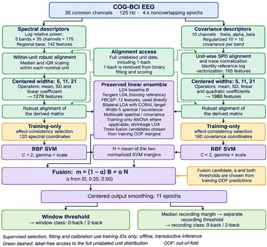
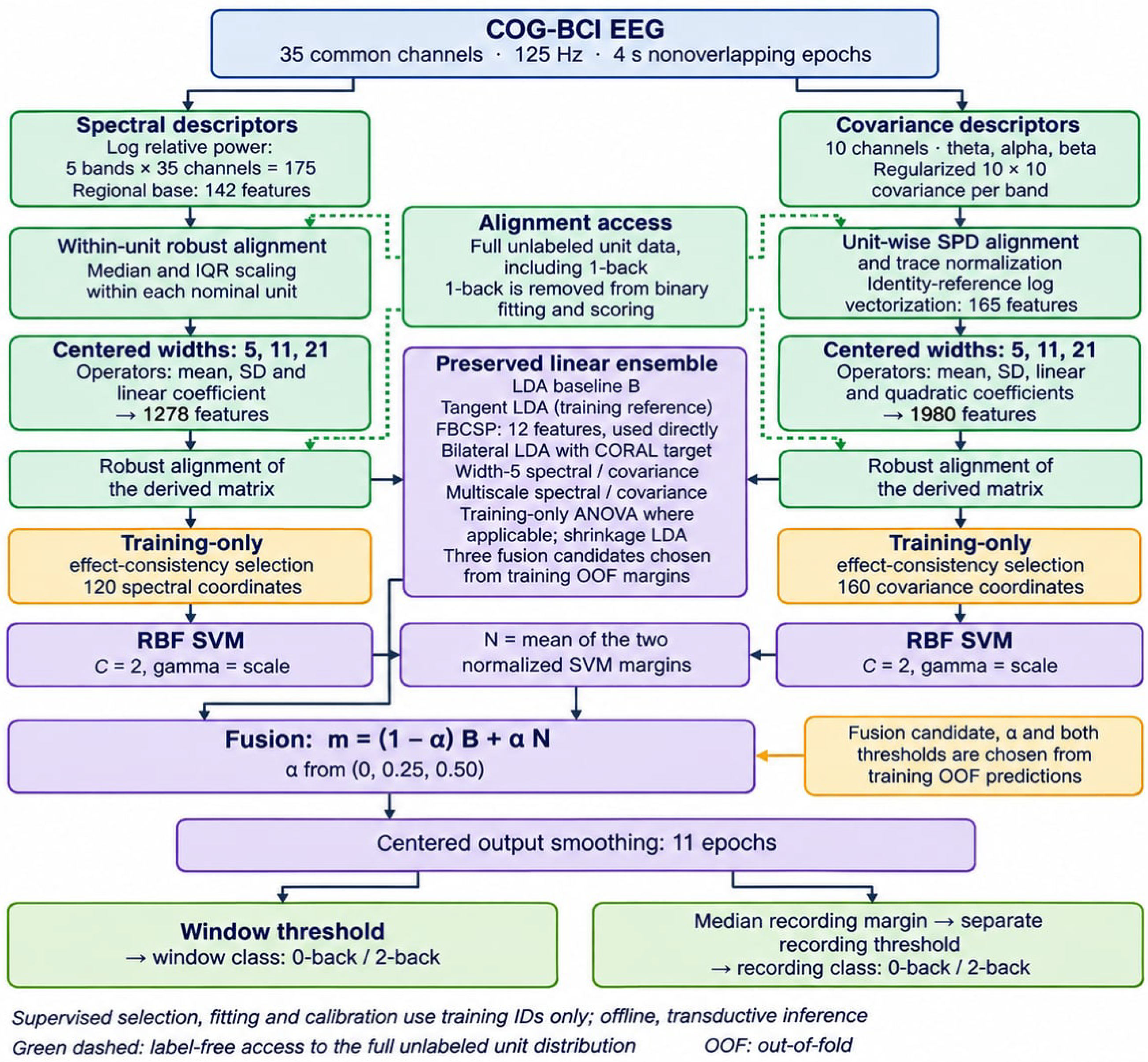
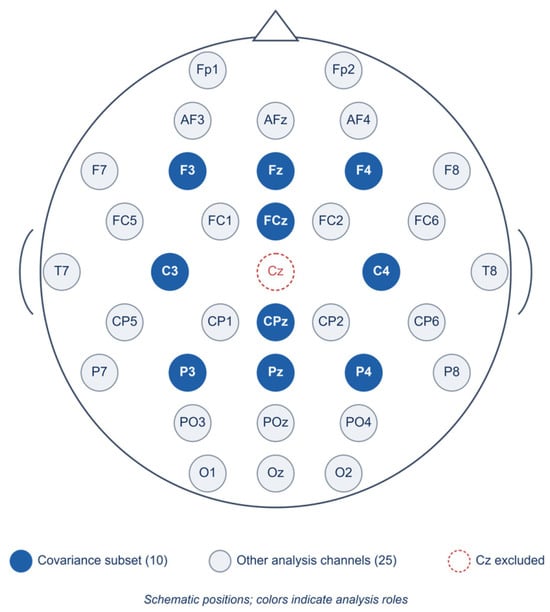
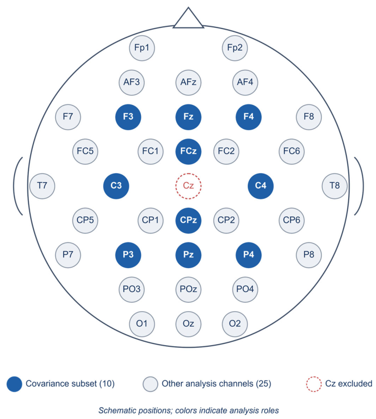
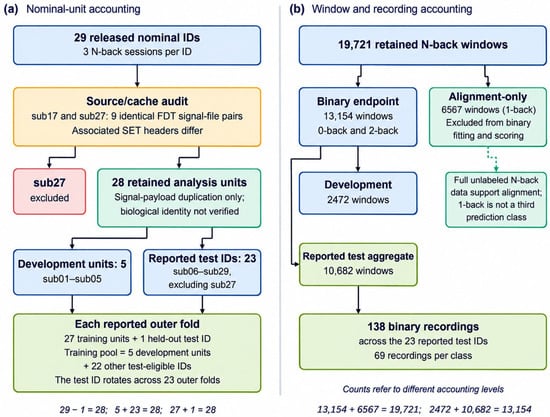
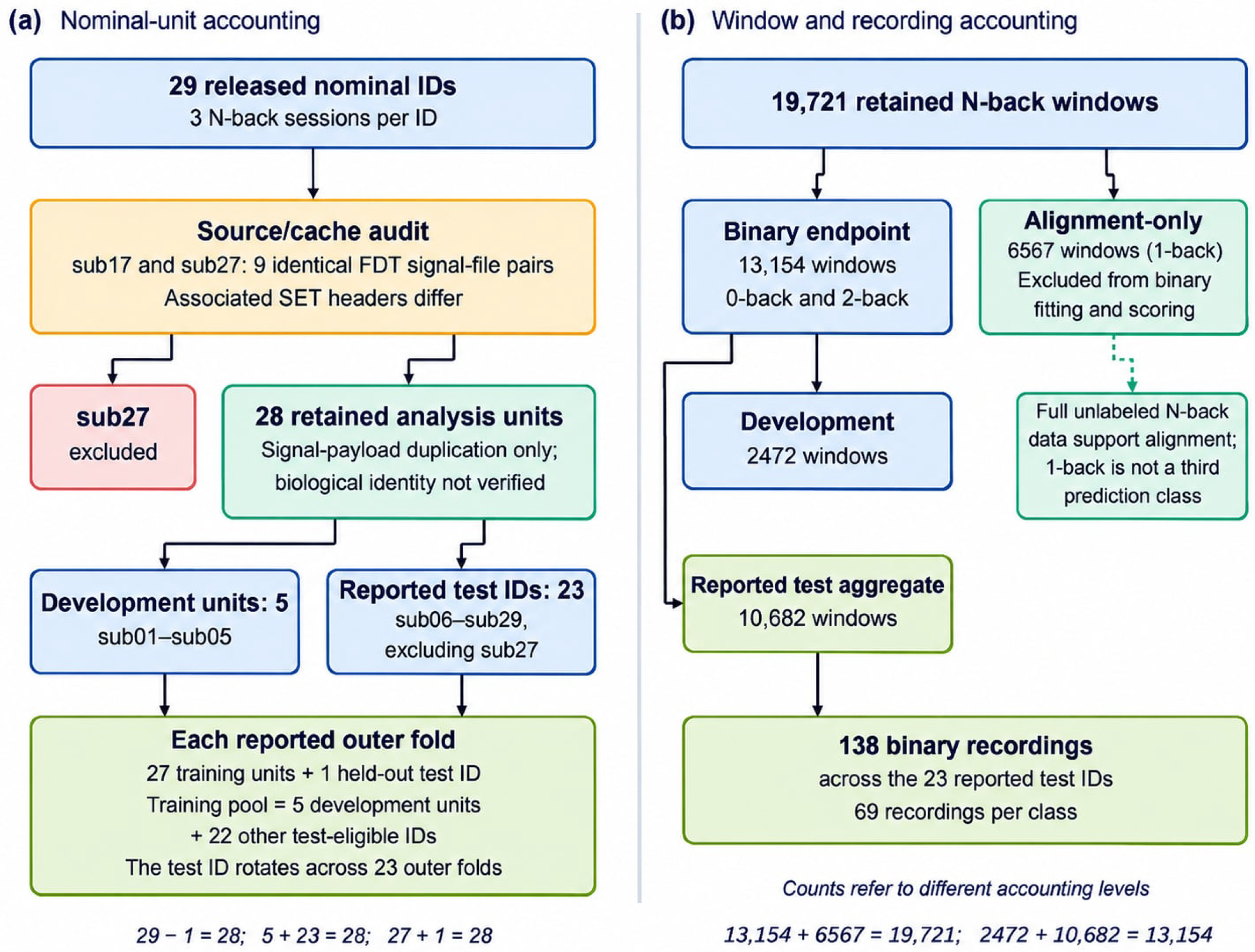
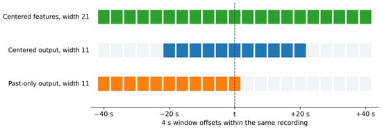
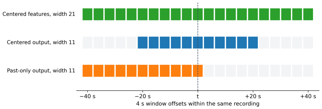
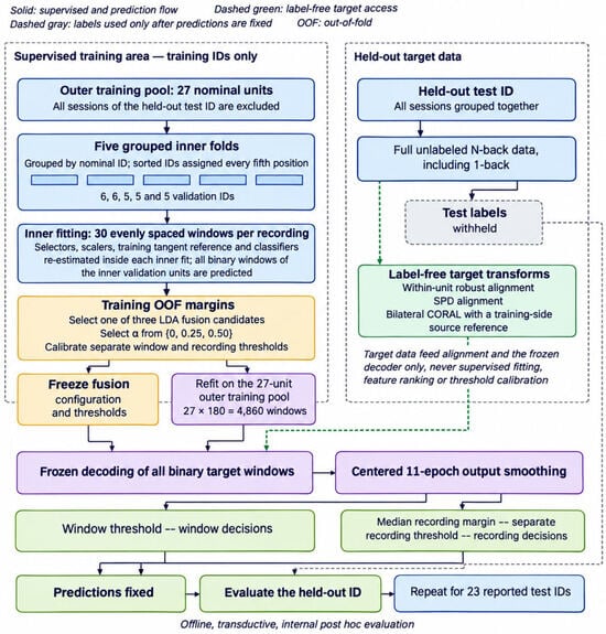
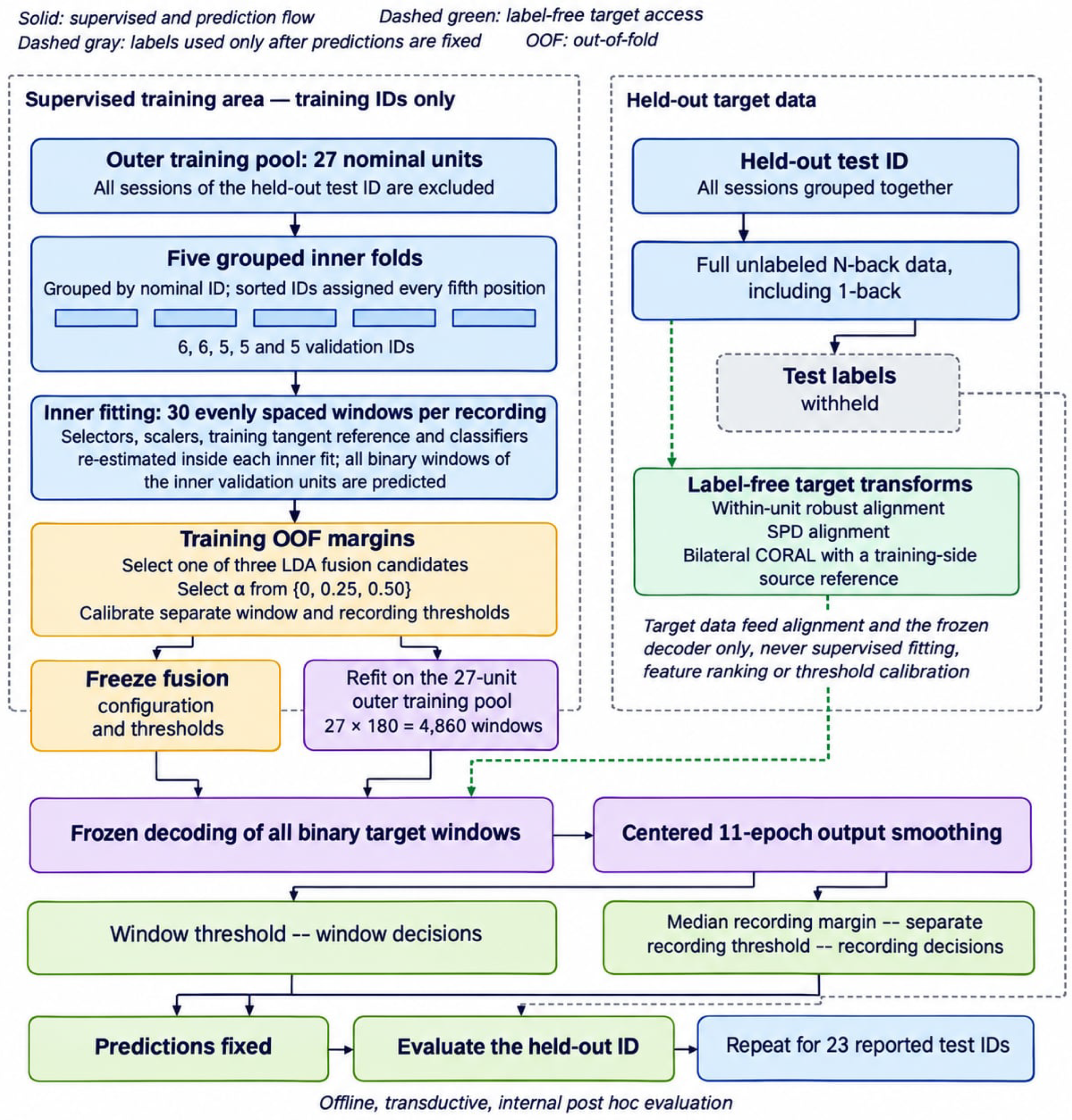
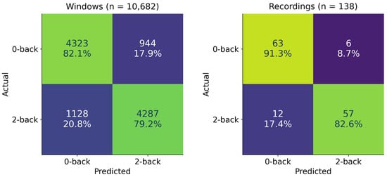
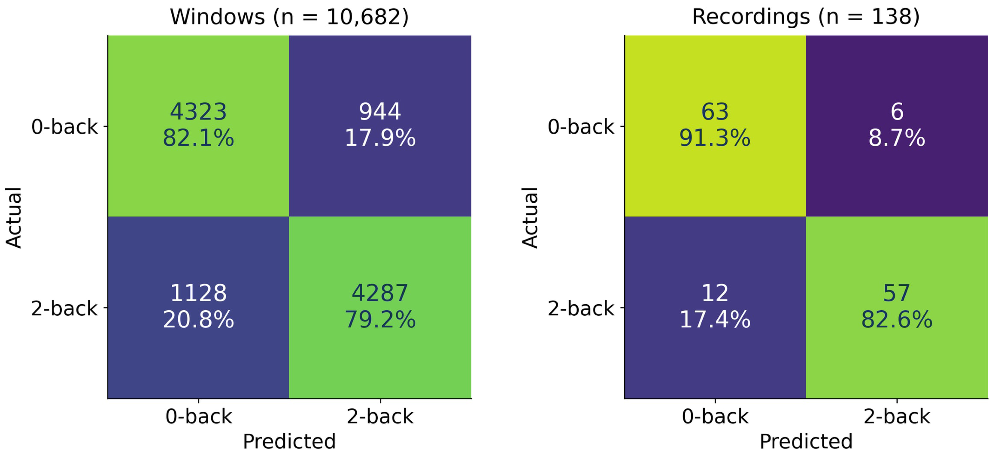
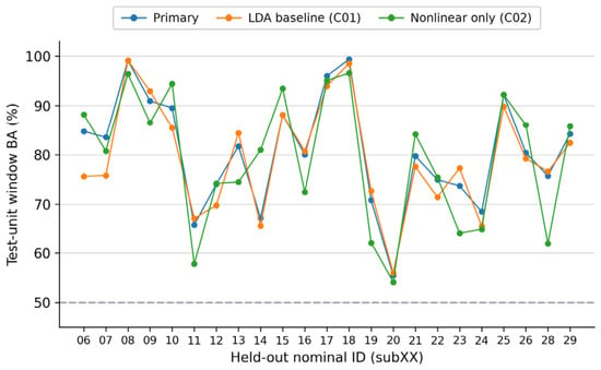
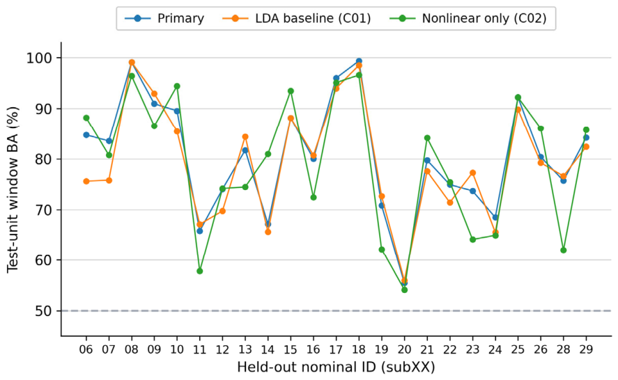
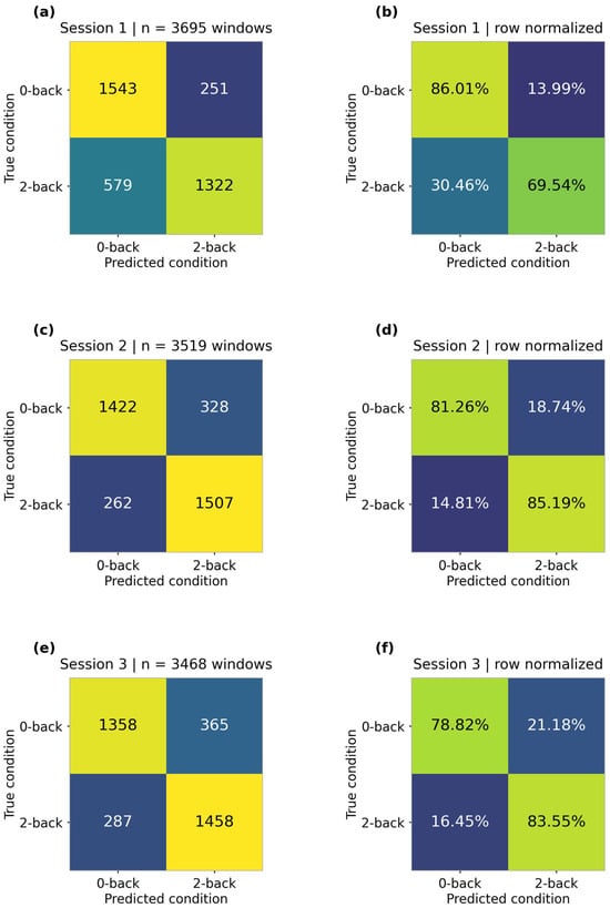
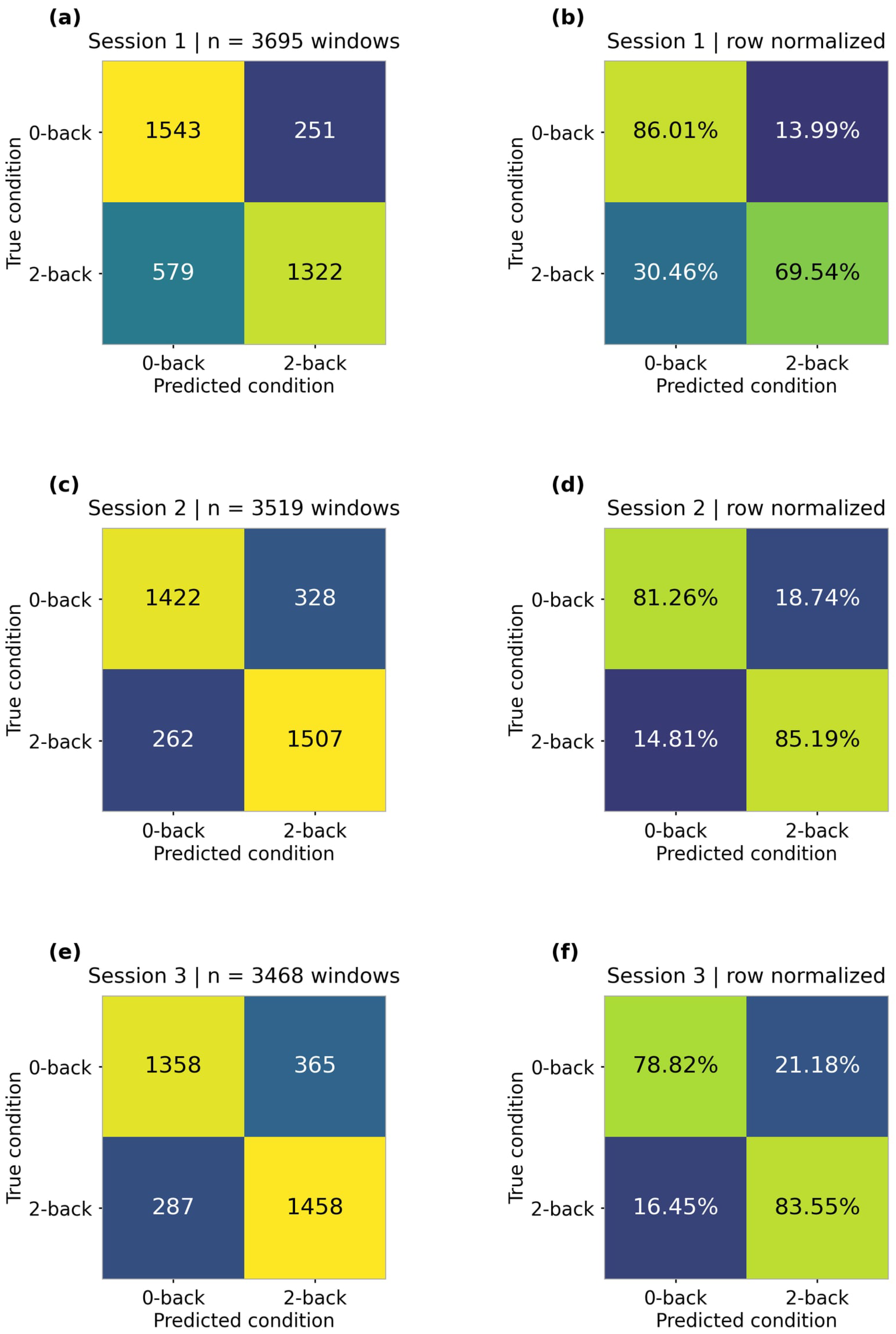
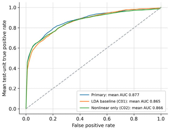
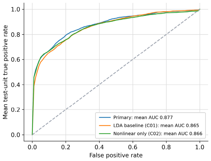
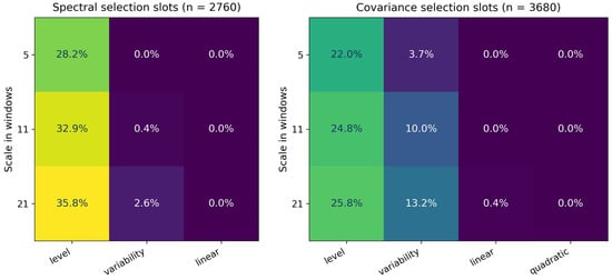
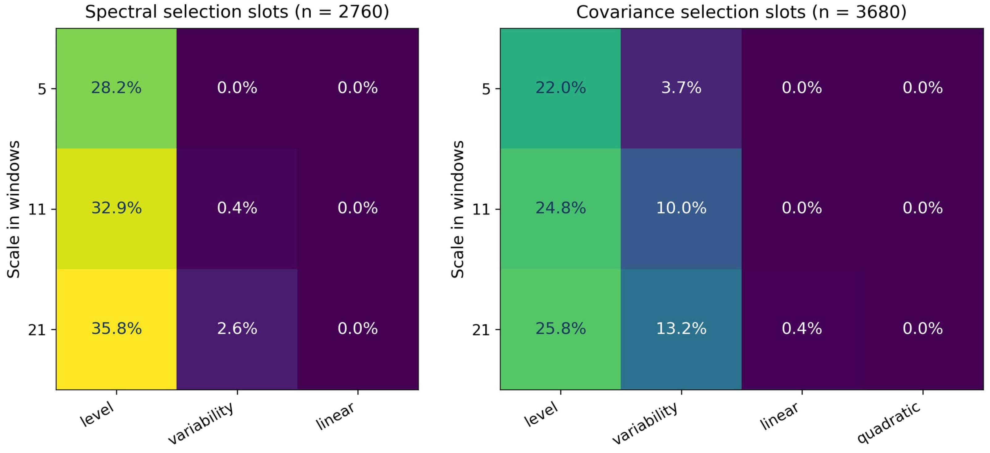
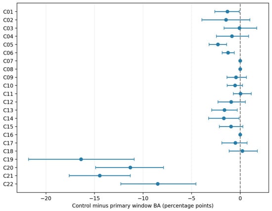
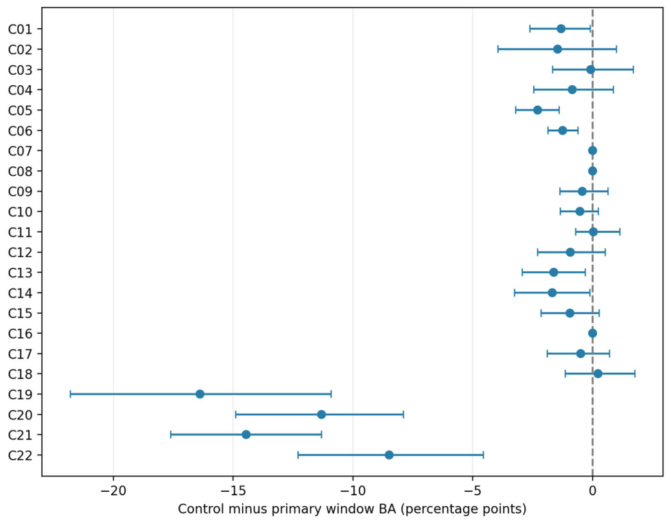

Disclaimer/Publisher’s Note: The statements, opinions and data contained in all publications are solely those of the individual author(s) and contributor(s) and not of MDPI and/or the editor(s). MDPI and/or the editor(s) disclaim responsibility for any injury to people or property resulting from any ideas, methods, instructions or products referred to in the content. |
© 2026 by the authors. Licensee MDPI, Basel, Switzerland. This article is an open access article distributed under the terms and conditions of the Creative Commons Attribution (CC BY) license.