


Abstract
Rainfall–runoff modeling is a key challenge in hydrological research. Despite the extensive application of long short-term memory (LSTM) networks in rainfall–runoff modeling, our understanding of the influence of different hyperparameter configurations on various hydrograph components, as well as the linkages between hydrological concepts and LSTM architectures, remains elusive. Here, we integrated Multi-Objective Particle Swarm Optimization (MOPSO) with LSTM hyperparameter optimization by targeting the root mean square error of the overall hydrograph (RMSEall), high-flow (RMSEhigh) and low-flow (RMSElow) dynamics, and water volume deviation (Dv). The MOPSO-LSTM framework was applied to the upstream catchments of the Miyun Reservoir in Beijing, China. At a lead time of 1d, the optimal solution achieved an NSE of 0.920 in the Chaohe River Basin, with a minimum RMSEall of 0.848 m3/s, RMSEhigh of 2.081 m3/s, RMSElow of 0.382 m3/s, and Dv of 0.002%. However, as the lead time increased to 3 and 7 days, the maximum NSE declined to 0.747 and 0.560, respectively, with process-related metrics deteriorating more substantially than water balance-related metrics. The Baihe River Basin performed better, with maximum NSE and KGE values of 0.949 and 0.970 at a lead time of 1d. Clear trade-offs among different evaluation objectives were further identified, particularly the competitive relationship between RMSEhigh and RMSElow, as well as the coupling between RMSElow and Dv. SHAP (Shapley additive explanation) and partial dependence plots (PDPs) were used to quantify and interpret the effects of hyperparameters on model performance, and the results showed that learning rate, number of units, and lookback window served as the most influential hyperparameters. Moreover, optimization preferences resulted in distinct hyperparameter configurations, where Dv-oriented solutions favored smaller learning rates, longer lookback windows, and larger batch sizes than RMSE-oriented solutions. Compared with the Chaohe River Basin, the larger Baihe River Basin favored LSTM configurations with longer lookback windows, more hidden units, higher learning rates, and lower dropout rates, which was associated with the hydrological memory of the catchment. Overall, this study provides a novel multi-objective LSTM optimization framework, improving the understanding of LSTM hyperparameters and offering practical guidance for hydrological prediction and water resource management.
1. Introduction
Rainfall–runoff modeling and forecasting provide critical support for water resource management and flood regulation [1]. However, in recent years, the intensification of climate change, land use changes, and human activities have contributed to pronounced non-stationarity, stochasticity, and spatiotemporal variability in rainfall–runoff processes, thereby increasing the difficulty of forecasting [2]. Physically based models, derived from rigorous hydrological and mathematical laws, exhibit strong physical consistency and reliability. However, they depend on considerable calibration efforts and expert knowledge, are subject to uncertainties in parameter estimation, and are constrained by rigid model structures that limit their ability to capture complex hydrological behaviors [3]. In contrast, machine learning models learn hydrological relationships between meteorological inputs and streamflow directly from data without explicit representation of hydrological processes, featuring convenient implementation and flexible architectures, and a strong capability to capture nonlinear processes in complex systems. Accordingly, they have been extensively adopted to rainfall–runoff modeling with promising performance and have become the hotspot of hydrology research [4,5].
The long short-term memory (LSTM) network with a multi-gate architecture, designed specifically for time-series modeling, addresses the vanishing gradient problem encountered by conventional RNNs when learning long-term dependencies, and its use has proven to be effective in hydrological forecasting [6]. For example, Frederik et al. [7] applied LSTM based on the CAMELS dataset to simulate streamflow processes across 241 catchments with diverse hydrological conditions in the United States, showing that the accuracy of simulated data was comparable to that of well-established process-based models. Martel et al. [8] employed LSTM to simulate streamflow under climate change scenarios across more than 1000 catchments in the United States, showing that it significantly outperformed conceptual hydrological models in terms of both the KGE and NSE metrics. However, machine learning models involve a large number of hyperparameters, and thus model performance critically depends on appropriate hyperparameter configuration. Neurons constitute the hidden layers and progressively transform and transmit information through the network during training [9]. The number of neurons depends on the complexity of the problem, as an excessive or insufficient number of hidden layers or neurons may lead to overfitting or underfitting [10]. Learning rate is a key hyperparameter of the Adaptive Moment Estimation (Adam) optimizer, which is widely used due to its simplicity and rapid convergence. However, setting it too small decelerates training, while too large a value risks divergence or suboptimal convergence [1]. In practice, learning rate tuning is more efficient on a logarithmic scale, which facilitates exponential decay and enables stable, systematic exploration of the parameter space. Batch size is dependent on the memory capacity of computational units (CPU/GPU) and controls the training speed. Larger batches accelerate training but risk degrading model quality when too large, while overly small batches may impede loss function convergence [11]. The dropout rate specifies the proportion of neurons randomly deactivated during training. It helps prevent overfitting and reduce generalization error by balancing training error, though its effectiveness depends on dataset characteristics and interactions with other hyperparameters [11]. Still, interpreting machine learning model results and understanding how hyperparameters influence model performance remain central challenges in hydrology [12].
In current practice, hyperparameter tuning for hydrological machine learning models relies largely on manual trial-and-error, a strategy that is not only experience-intensive but also prone to suboptimal outcomes. Some studies have gone further by adopting random search methods for LSTM hyperparameter optimization [13]. Nevertheless, they remain constrained by the use of a single performance metric, while multi-objective optimization approaches are still limited, particularly those considering different components of hydrological processes, which inevitably compromises the model’s capacity to balance streamflow dynamics with water balance consistency [14]. NSE is one of the most popular evaluation metrics, and its importance is often taken for granted [15]. However, it is particularly sensitive to high-flow extremes while being relatively insensitive to systematic overestimation or underestimation, which often leads to a model’s poor performance in low flows and substantial water balance bias [16]. For instance, Xu et al. [14] used a particle swarm optimization algorithm with NSE as the sole objective function to tune several hyperparameters, and their results demonstrated that though NSE remained around 0.7 for longer lead times, the percent bias approached 50%. Amirmasoud et al. [1] applied random search and tree-structured Parzen estimators to tune hyperparameters of DNN, CNN, and LSTM models with RMSE over the full simulation period as the objective and found that different hyperparameter configuration strategies yielded varying performances under different rainfall intensities, hindering the simultaneous representation of both high- and low-flow conditions. Therefore, multi-objective optimization of the LSTM model should be further explored to obtain optimal hyperparameters across different aspects of model performance.
As for the interpretation of hydrological modeling results, a few studies have employed SHAP and PDP methods to quantify the contributions of parameters to model performance [12,17,18]. However, they have mainly focused on the relationship between hyperparameters and overall predictive performance, while the influences of hyperparameter configurations on different hydrograph components, including overall streamflow dynamics, high-flow and low-flow processes, and water balance preservation, across multiple lead times remain largely unexplored. Multi-Objective Particle Swarm Optimization (MOPSO) is a representative heuristic multi-objective optimization algorithm [19,20], and it has demonstrated effectiveness in hydrological parameter optimization [21]. To address this gap, we speculate that further interpretation of the MOPSO-LSTM optimization results by using SHAP and PDPs may help establish linkages between hyperparameter configurations and hydrological behavior, particularly the responses of different components of the hydrograph. Theoretically, this framework can underpin practical water resource management, as distinct objectives call for tailored model architectures and hyperparameter configurations. For instance, reservoir operation and water supply management tend to focus on medium- to long-term inflows and drought conditions associated with low flows, whereas flood control is primarily concerned with short-term high-flow events and flood risks.
Our study focusses on the upstream catchments of Miyun Reservoir, which is an important surface drinking water source for Beijing, China. The upstream runoff directly affects flood safety, water supply security, and ecological regulation in the capital region. At present, process-based hydrological models are relatively well established in those basins, with most studies focusing on models such as SWAT [22] and HSPF [23]. However, in recent years, with changing precipitation regimes and intensified human activities in this region, the non-stationary characteristics of upstream inflows have become increasingly pronounced [22]. Traditional process-based models show limited capability in responding to complex rainfall conditions, whereas the application of machine learning models in this region remains relatively scarce. We therefore established a MOPSO-LSTM framework in this region to (1) characterize the trade-offs among different optimization objectives in LSTM rainfall–runoff modeling; (2) identify variations in optimal hyperparameter configurations under different lead times and optimization objectives; and (3) interpret the relationships between hyperparameter configurations and the representation of different hydrological behaviors.
2. Materials and Methods
2.1. Case Study and Dataset
The upstream watershed of the Miyun Reservoir (115.4°~117.5° E, 40.4°~41.6° N) is located in the northern part of Beijing, with elevations mostly ranging from 500 to 2000 m and a predominantly mountainous terrain. This region lies within a continental monsoon climate zone, characterized by cold and dry weather in winter, but it is rainy and hot in summer. The long-term mean annual temperature is 10.5 °C, and the mean annual precipitation is approximately 500 mm, with 80% of the rainfall occurring from July to September. Xiahui and Zhangjiafen hydrological stations serve as their respective control stations [24]. Based on the 30 m resolution digital elevation model (DEM) downloaded from the Geospatial Data Cloud (https://www.gscloud.cn/), we used the ArcSWAT 2012.10.26 tool to delineate the watershed boundaries and extract the river networks. Subsequently, the catchment area, trunk stream length, catchment perimeter, mean elevation, and mean slope of the Chaohe River and Baihe River Basins were calculated, as summarized in Table 1.
Table 1.
Summary of the basic characteristics of the Chaohe River and Baihe River Basins.
Figure 1 demonstrates the study area and the location of hydrometric stations and rainfall gauged stations. Observed daily streamflow data from the Xiahui hydrometric station and daily precipitation data from 10 rainfall gauged stations in the Chaohe River Basin were collected from 2000 to 2017. The data from 2000 to 2012 were used for calibration, while those from 2013 to 2017 were used for validation. To further evaluate the applicability of LSTM in the upstream watershed of the Miyun Reservoir, observed daily streamflow data at the Zhangjiafen hydrometric station and concurrent daily precipitation data from 17 rainfall stations in the Baihe River Basin were also collected from 2000 to 2010. The data from 2000 to 2006 were used for calibration, and those from 2007 to 2010 were used for validation. The split-ratio of the calibration and validation dataset was approximately 7:3. Further, based on the historical streamflow records, the baseflow index (BFI) and streamflow autocorrelation functions (ACFs) at lag times of 1, 3, and 7 days were calculated for the two basins, as summarized in Table 1. Detailed descriptions of the calculation methods for BFI and ACFs are provided in Supplementary Material Texts S1 and S2, respectively.
Figure 1.
Overview of the study area. (a) Distribution of the Chaohe River Basin, Baihe River Basin, rain gauged stations, and hydrometric stations. The inset in the upper-right corner shows the location of the upstream watershed of the Miyun Reservoir within China. (b) Elevation distribution of the upstream watershed of the Miyun Reservoir. The inset in the upper-right corner shows the location of the upstream watershed relative to Beijing.
2.2. Long Short-Term Memory (LSTM) Rainfall–Runoff Model
Long short-term memory (LSTM) neural networks, as a special type of Recurrent Neural Network (RNN), address the problems of vanishing and exploding gradients during training by replacing the traditional recurrent units with memory cell units. Figure 2 shows the structure of the memory cell unit in the hidden layer of LSTM [25]. An LSTM consists of an input layer, one or more hidden layers, and an output layer. By introducing a forget gate, input gate, output gate, and cell state, the memory cell in the hidden layer can selectively remember and forget information from the input data. Specifically, the input gate controls the extent to which the current input information updates the memory state. The forget gate regulates the retention and discarding of historical information, thereby determining how long information is preserved within the memory cell. The output gate controls the contribution of the current memory state to the model output, enabling the effective modeling of long-term dependencies in sequential data [26]. In this study, precipitation data and historical runoff are used as input features, while streamflow at the Xiahui and Zhangjiafen stations is used as the output variable to train the LSTM prediction model. To investigate differences in model performance across lead times, the lead times were set to 1, 3, and 7 days, respectively. To further mitigate overfitting, the LSTM model was trained for a maximum of 200 epochs with an early stopping strategy based on validation loss, using a patience of 20 epochs (Δ < 0.5%).
Figure 2.
The internal operation of the LSTM block [25].
2.3. Hyperparameter Optimization Based on Multi-Objective Particle Swarm Optimization (MOPSO)
Hyperparameter optimization can effectively improve the performance of deep learning-based hydrological models. For instance, Amini et al. employed a random search approach to optimize nine hyperparameters, including the number of hidden units, lookback, learning rate, activation function, and other training-related parameters, and evaluated the performance of multivariate deep learning-based rainfall nowcasting models using NSE and RMSE. Their sensitivity analysis further identified lookback, learning rate, and batch size as the most influential hyperparameters [1]. Xu et al. applied the particle swarm optimization (PSO) algorithm to optimize three key hyperparameters (batch size, lookback, and number of units) of LSTM models for rainfall–runoff forecasting with lead times ranging from 1 to 12 h. The corresponding search ranges were set as [24, 128], [4, 8], and [32, 256], respectively, with a population size of 30 and 100 iterations [14]. Huseyin et al. employed PSO to optimize the hyperparameters of a hybrid Bayesian–ConvLSTM model for hydrological time-series forecasting, including convolutional filter learning rates (0.001, 0.01, and 0.1) and LSTM units (32, 64, and 128), using a swarm size of 5 and a maximum of 5 iterations [27]. Building upon previous findings, we selected the most relevant hyperparameters and determined their search spaces by considering both the recommendations from previous studies and the characteristics of the rainfall–runoff time series in the study area.
Multi-Objective Particle Swarm Optimization (MOPSO) is an evolutionary optimization algorithm that solves optimization problems involving multiple conflicting objectives by constructing a Pareto-optimal set, which consists of a group of non-dominated solutions representing different trade-offs among the objectives [28]. In this study, an improved MOPSO algorithm incorporating the crowding distance strategy was adopted. An external archive was introduced to preserve elite particles, while particles with larger crowding distances were preferentially retained to maintain population diversity. A linearly decreasing inertia weight was further employed to achieve a dynamic balance between global exploration and local exploitation. To identify the optimal hyperparameter configuration for the LSTM model, MOPSO was used to optimize the major hyperparameters, with the hydrological performance metrics evaluated on the validation dataset serving as the objective functions. Following previous studies, the swarm size and the maximum number of iterations were set to 40 and 100, respectively [14]. The inertia weight was linearly decreased from 0.9 to 0.4, while both the cognitive and social learning factors (c1 and c2) were set to 1.5. To evaluate the convergence behavior and optimization performance of MOPSO, the hypervolume (HV) and inverted generational distance (IGD) metrics were calculated at each iteration. Detailed descriptions and calculation of these metrics are provided in Supplementary Material Text S3. Based on the multi-objective relationships between hyperparameter configurations and different aspects of hydrological processes, this study develops a novel MOPSO–LSTM framework for rainfall–runoff forecasting. All training–optimization experiments were conducted on a PC running Windows 11, equipped with an NVIDIA GeForce RTX 4060 Laptop GPU (8 GB VRAM). The deep learning framework was implemented using PyTorch 2.5.1 with CUDA 12.4 and cuDNN 9.1.0. The detailed settings of the MOPSO-LSTM method are summarized in the following subsection.
2.3.1. Decision Variables
Five key hyperparameters were selected as decision variables: batch size, number of hidden units, lookback window, dropout rate, and learning rate. Based on the characteristics of the rainfall–runoff time series, the LSTM model was configured with a single hidden layer [7,29,30,31]. Batch size, defined as the number of samples processed in each training iteration, was optimized over a range of 8 to 256 with an interval of 8. The number of units was searched over integers ranging from 10 to 200 with an interval of 10. The learning rate, which controls the step size during gradient descent optimization of the loss function, was selected from [0.0001, 0.001, 0.01]. The dropout rate ranged from 0.1 to 0.5 with an interval of 0.1 [1]. The lookback window, defined as the number of historical hydro-meteorological input time steps used to predict streamflow at the next time step, was searched over integer values from 1 to 40 [32].
2.3.2. Objective Functions
To comprehensively evaluate the performance of the LSTM rainfall–runoff model in simulating different flow regimes and water balance, the objective functions of MOPSO include the root mean square error of the entire flow series (RMSEall), the root mean square error of high-flow conditions (RMSEhigh), the root mean square error of low-flow conditions (RMSElow), and water volume deviations (Dv). Here, RMSEhigh and RMSElow represent the high-flow and low-flow segments of the hydrological process, respectively. The high-flow segment (0~10% flow exceedance probabilities) represents rapid catchment responses to precipitation events, while the low-flow segment (10%~100%) represents the remaining flow conditions, which are mainly related to long-term sustainability and controlled by slower hydrological components, such as baseflow [33,34]. The high-flow quantile threshold was selected based on previous studies, which demonstrated that a 10% exceedance probability threshold is effective for identifying high-flow components and evaluating model performance under high-flow conditions [35,36,37]. Accordingly, in this study, “low-flow” denotes the remaining flow conditions after excluding the highest 10% high-flow segment, corresponding to the 10~100% flow-exceedance range.
The formulations are detailed as follows:
where (m3/s) represents the root mean square error for the entire flow series, (m3/s) denotes the observed daily mean discharge on day i, (m3/s) signifies the predicted discharge by LSTM on day i, and N is the total number of time steps.
where (m3/s) represents the root mean square error for high-flow conditions. High-flow conditions were defined as discharge values greater than or equal to the 90th percentile (). represents the number of samples with .
where (m3/s) represents the root mean square error for low-flow conditions. Low-flow conditions were defined as discharge values less than the 90th percentile (). represents the number of samples with .
where Dv (%) represents the total water volume deviation, and Δt represents the time step, which is 1 day.
2.3.3. Evaluation Metrics
Additionally, the commonly used Nash–Sutcliffe efficiency (NSE) and Kling–Gupta efficiency (KGE) metrics were used to comprehensively evaluate model performance, which are calculated as follows:
where (m3/s) means the observed daily mean discharge on day i; is average observed discharge (m3/s); (m3/s) represents the predicted discharge on day i; and N is the total number of time steps.
where r represents the Pearson correlation coefficient between simulated and observed values, α is the ratio of the mean of simulated values to the mean of observed values, and β is the ratio of the standard deviation of simulated values to the standard deviation of observed values [38].
Furthermore, Pearson correlation analysis was employed to evaluate the relationships among the above evaluation metrics for the predicted streamflow processes of the Pareto front solutions. The workflow of the MOPSO-LSTM approach is shown in Figure 3.
Figure 3.
Schematic diagram of MOPSO-LSTM. The text in blue indicates the specific parameters or metrics involved in each step.
2.4. SHAP and PDP for Interpretation of LSTM Performance
The Shapley additive explanation (SHAP) method was adopted to quantify the effects of different hyperparameters on LSTM rainfall–runoff model performance. SHAP is derived from Shapley value theory in cooperative game theory and explains complex machine learning models by computing the marginal contribution of each input feature to the model output [18,39]. When dealing with large datasets and high-dimensional hyperparameter spaces, evaluating every possible hyperparameter configuration to construct a dataset for SHAP analysis was unnecessary and computationally inefficient [40]. Therefore, we employed Latin hypercube sampling (LHS) to sample the hyperparameter space and construct a representative dataset, which has been combined with SHAP analysis to explore variable contributions in complex parameter spaces in previous studies [41]. LHS promotes approximately uniform coverage of the marginal distribution of each hyperparameter, thereby achieving broad coverage of the hyperparameter space with a relatively small number of samples [42]. An LSTM model was independently trained and evaluated for each sampled hyperparameter configuration. The sampled hyperparameters were then used as the input features, while the corresponding model evaluation metrics were used as the output features in the subsequent surrogate-model-based SHAP analysis. For the sample i (), the predicted value of the metric is , and the average value of this metric is . The hyperparameter k is . Then, the SHAP value is calculated as follows:
where represents the contribution of hyperparameter k to . By calculating the mean absolute SHAP values, the influence of batch size, units, lookback window, dropout rate, and learning rate on model performance can be quantitatively evaluated. A larger SHAP value indicates a greater contribution of the hyperparameter to model performance.
Furthermore, partial dependence plots (PDPs) were used to reveal how each attribute affects the prediction results of the LSTM model. PDPs quantify the change in model outputs by varying the target feature while holding all other non-target features constant. In the PDP analysis, the hyperparameter spaces of the learning rate and dropout rate were refined by adding intermediate values to better capture local variations in response patterns. The refined learning rate values were [1 × 10⁻⁴, 3 × 10⁻⁴, 5 × 10⁻⁴, 7 × 10⁻⁴, 1 × 10⁻³, 3 × 10⁻³, 5 × 10⁻³, 7 × 10⁻³, 1 × 10⁻²], and the refined dropout rate values were [0.1, 0.13, 0.15, 0.17, 0.2, 0.23, 0.25, 0.27, 0.3, 0.33, 0.35, 0.37, 0.4, 0.43, 0.45, 0.47, 0.5].
where denotes the hyperparameter of interest, represents the set of all other hyperparameters is the response function that maps hyperparameters to metric M, and is the model’s overall feature probability density [43].
3. Results
3.1. MOPSO of the LSTM Model Under Different Lead Times
During the calibration and validation periods, the daily discharge at the Xiahui station in the Chaohe River Basin ranged from 0.071 to 99.8 m3/s and from 0.16 to 33.4 m3/s, with mean values of 2.97 and 3.41 m3/s, respectively. For lead times of 1, 3, and 7 days, the MOPSO-LSTM model obtained 43, 59, and 98 Pareto-optimal solutions after 36.46 h, 42.90 h, and 54.35 h of training and optimization, respectively. The HV and IGD convergence curves, as well as computational time, are presented in Supplementary Material Figures S1–S3. The distributions and ranges of the four metrics on the Pareto front are shown in Figure 4 and Figure 5, respectively. For lead times of 1, 3, and 7 days, the validation RMSEall ranged from 0.848 to 1.083 m3/s, 1.504 to 1.700 m3/s, and 1.985 to 2.157 m3/s, respectively. The corresponding RMSEhigh ranged from 2.081 to 2.824 m3/s, 3.678 to 4.660 m3/s, and 5.213 to 6.208 m3/s, while RMSElow ranged from 0.382 to 0.775 m3/s, 0.629 to 1.272 m3/s, and 0.699 to 1.425 m3/s, and the Dv ranged from 0.002% to 6.913%, 0.002% to 7.667%, and 0.003% to 8.887%, respectively. In addition, the commonly used performance metrics NSE and KGE were also evaluated. For lead times of 1, 3, and 7 days, NSE ranged from 0.869 to 0.920, 0.677 to 0.747, and 0.480 to 0.560, respectively, while KGE ranged from 0.838 to 0.950, 0.629 to 0.827, and 0.510 to 0.686.
Figure 4.
Pareto fronts obtained from MOPSO-LSTM model with lead times of 1d (a), 3d (b), and 7d (c). The four-dimensional Pareto front is visualized with RMSEall, RMSEhigh, and RMSElow on the X-axis, Y-axis, and Z-axis, respectively, and Dv is represented by the color mapping. The point Sall and the vertical lines projected onto the X-Y-Z-axes represent the Pareto solution with the minimum RMSEall. Similarly, Shigh and Slow indicate the Pareto solutions with the minimum RMSEhigh and RMSElow, respectively. The coordinates of these points are expressed as RMSEall, RMSEhigh, RMSElow, and Dv.
Figure 5.
The ranges of hydrological performance metrics in the Pareto-optimal solution sets under different lead times. (a) RMSEall, (b) RMSEhigh, (c) RMSElow, (d) Dv, (e) NSE, and (f) KGE.
It can be seen that model performance deteriorated as the lead time increased. Specifically, from 1 to 3 days, the mean values of RMSEall, RMSEhigh, and RMSElow across the Pareto-optimal solutions increased by 64.06%, 67.86%, and 56.67%, respectively. Additionally, NSE and KGE decreased by 19.21% and 16.92%, respectively. From 3 to 7 days, the mean values of RMSEall, RMSEhigh, and RMSElow increased by 30.05%, 37.22%, and 10.95%, respectively. Meanwhile, NSE and KGE decreased by 26.16% and 20.87%, respectively. However, Dv changed only slightly, with average Dv values of 1.037%, 1.560%, and 1.601% at lead times of 1, 3, and 7 days, respectively. Compared with the transition from 1 to 3 days, the decreases in NSE and KGE were slightly greater from 3 to 7 days, while the increases in RMSEall, RMSEhigh, and RMSElow were approximately halved. However, the increase in Dv was substantially reduced.
3.2. Multi-Objective Trade-Offs Among Hydrological Evaluation Metrics
From the Pareto fronts, the preference-based solutions for RMSEall, RMSEhigh, RMSElow, and Dv were selected and denoted as Sall, Shigh, Slow, and SDv, respectively. The predicted and observed hydrographs of different solutions are shown in Figure 6, and the corresponding parameter settings are listed in Table 2. Sall mainly exhibited overestimation of low-flow conditions and underestimation of high-flow conditions. Shigh yielded lower RMSEhigh than other solutions, indicating superior performance in high-flow prediction. At a lead of 1 day, Shigh accurately predicted the flood peaks on 17 July 2013 and 25 July 2016, with observed peak discharges of 30.0 m3/s and 30.6 m3/s, and simulated peak values of 28.13 m3/s and 30.76 m3/s, respectively. In comparison, Sall, Slow, and SDv produced peak discharges of 25.39 m3/s, 23.82 m3/s, and 21.13 m3/s for the 2013 event, and 27.63 m3/s, 23.09 m3/s, and 27.56 m3/s for the 2016 event, respectively. Slow showed better performance in simulating low-flow conditions but generally underestimating high-flow events. SDv exhibited limited variation in Dv across different lead times, indicating relatively stable water balance performance.
Figure 6.
Comparison of predicted and observed streamflow hydrographs in the Chaohe River Basin for the preference-based solutions for RMSEall, RMSEhigh, RMSElow, and Dv. Lead times of (a) 1d, (b) 3d, and (c) 7d.
Table 2.
Performance metrics and corresponding hyperparameter values for different preference-based solutions under different lead times in the Chaohe River Basin.
Furthermore, Pearson correlation analysis was conducted to examine the relationships between the different evaluation metrics, as shown in Figure 7 and Supplementary Material Table S1. At a lead time of 1 day, RMSEall showed a significantly positive correlation with both RMSEhigh and RMSElow. Across all lead times, RMSElow and RMSEhigh exhibited significant negative correlations. In particular, RMSElow was also predominantly negatively correlated with NSE. In contrast, Dv mainly demonstrated negative correlations with RMSEall and RMSEhigh but positive correlations with RMSElow. Additionally, KGE showed a significant negative correlation with RMSEhigh and a significant positive correlation with RMSElow across all lead times. These indicate clear trade-offs among different evaluation metrics, suggesting that the traditional practice of evaluating model performance using a single metric is highly limited.
Figure 7.
Heatmap of Pearson correlations among six hydrological evaluation metrics. Lead time of (a) 1d, (b) 3d, and (c) 7d. “*” indicates statistically significant correlations (p < 0.05). Only the lower triangular matrix is shown, as the upper triangular matrix is identical due to symmetry.
Distinctive patterns of hyperparameter combinations were observed under different lead times and optimization preferences. Learning rate generally declined with increasing lead times, decreasing from 0.001~0.01 for the 1-day and 3-day lead times to 0.0001~0.01 for the 7-day lead time. Among different preference strategies, the SDv solutions consistently adopted smaller learning rates compared with the RMSE preference-based solutions. Batch size primarily varied among different optimization preferences. SDv tends to adopt larger batch sizes; for example, at a lead time of 3 days, the batch size reaches 216, whereas the maximum batch size among RMSE preference-based solutions was 72. The lookback window was relatively large for both SDV and Slow at the lead times of 1 day and 7 days, whereas smaller values were selected at the lead time of 3 days. Similarly, the number of units was larger for the RMSE preference-based solutions compared with SDv at the lead times of 1 day and 7 days, while an opposite tendency is observed at the 3-day lead time. The dropout parameter reached its highest value of 0.5 in the DV preference-based solution.
3.3. Interpretability Analysis of the LSTM Model Using SHAP and PDP
The effects of hyperparameters on model performance with different lead times were interpreted using the SHAP method, as shown in Figure 8. Overall, the learning rate was consistently identified as the most influential hyperparameter across nearly all lead times, with a particularly strong effect on RMSElow. For the lead time of 1 day, lower learning rates tended to increase RMSEall, RMSEhigh, and RMSElow while reducing Dv. In contrast, for the lead times of 3 days and 7 days, lower learning rates generally tended to decrease RMSEall, RMSEhigh, and Dv. As lead time increased, the importance of the lookback window became more pronounced. For lead times of 3 days and 7 days, the contribution of lookback window ranked first or second, whereas for the 1-day lead time, batch size showed relatively higher importance. Batch size exhibits moderate importance, with its influence varying across optimization objectives and slightly higher importance observed for RMSElow and Dv. Similarly, units exhibited lower importance. However, for RMSEhigh at a lead time of 1 day, it became the most important hyperparameter, and the dropout rate consistently showed the lowest importance among all hyperparameters.
Figure 8.
SHAP summary plots and the importance ranking for the 5 LSTM hyperparameters across Chaohe River Basin. Lead times of (a) 1d, (b) 3d, and (c) 7d. In the SHAP plots, each dot represents one LSTM hyperparameter configuration, with color gradients showing feature magnitudes (red: high; blue: low). The SHAP value axis indicates feature positive and negative contributions to test performance metrics. In the bar plots, feature importance is defined as the mean absolute SHAP value (mean |SHAP value|) of each hyperparameter.
Partial dependence plots (PDPs) were further applied. For clarity, only the effects of the hyperparameters on NSE are presented in the main text (Figure 9), while the corresponding results for the other evaluation metrics are provided in the Supplementary Material Figures S4–S7. For a lead time of 1 day, NSE increased with increasing learning rate and gradually plateaued at higher learning rates. In contrast, for the 3-day and 7-day lead times, the highest NSE was achieved at intermediate learning rates, while both excessively high and low learning rates reduced model performance. Similar response patterns were observed for the RMSE-based metrics. By contrast, Dv exhibited an initial decrease followed by an increase at the 1-day lead time, whereas a monotonic increasing trend was observed at the 3-day and 7-day lead times, indicating that the learning rate resulted in poorer Dv performance. Compared with the learning rate, batch size had a weaker effect on NSE, resulting in a smaller variation in the objective values. For units, NSE generally increased initially and then decreased across all lead times. Among all hyperparameters, the lookback window exhibited the strongest dependence on lead time. At a lead time of 1 day, NSE decreased with increasing lookback window. At a lead time of 3 days, NSE first decreased and then increased, gradually reaching a plateau when the lookback window exceeded approximately 10~15 days. In contrast, at a lead time of 7 days, NSE increased continuously with increasing lookback window, suggesting that incorporating longer historical input sequences improves predictive performance for longer lead times. For the dropout rate, NSE changed slightly across all lead times, indicating the limited effects of this hyperparameter on model performance.
Figure 9.
Partial dependence plots of LSTM hyperparameters for NSE under different lead times. (a) 1d, (b) 3d, and (c) 7d. The X-axis represents hyperparameter values, and the Y-axis represents the simulated performance metric under averaged effects of other hyperparameters.
3.4. Application and Comparative Analysis of the MOPSO-LSTM in the Baihe River Basin
To evaluate the applicability of the MOPSO-LSTM model in the upstream Miyun Reservoir, the model was further applied to the spatially adjacent Baihe River Basin. The predicted streamflow under different preference solutions in the Pareto front is shown in Figure 10. At the Zhangjiafen station in the Baihe River Basin, the daily streamflow ranged from 0.077 to 94.2 m3/s in the calibration period and 0.39 to 108 m3/s in the validation period, with average values of 5.23 m3/s and 6.56 m3/s, respectively, approximately twice those observed at the Xiahuai station in the Chaohe River Basin. The optimization results showed that RMSEall, RMSEhigh, RMSElow, and Dv in the Baihe River Basin were generally 2~3 times higher than those in the Chaohe River Basin, which was mainly attributed to the higher streamflow at this site. While NSE and KGE were even better in the Baihe River Basin, reaching maximum values of 0.949 and 0.970 at a lead time of 1d, 0.756 and 0.829 at a lead time of 3d, and 0.632 and 0.729 at a lead time of 7d, respectively. These results suggest that the MOPSO-LSTM achieved better performance in the Baihe River Basin.
Figure 10.
Comparison of predicted and observed streamflow hydrographs in the Baihe River Basin for the preference-based solutions for RMSEall, RMSEhigh, RMSElow, and Dv. Lead times of (a) 1d, (b) 3d, and (c) 7d.
The optimal hyperparameter configurations are provided in Table 3. Notable differences in optimal hyperparameter configurations were observed between the Baihe and Chaohe River Basins. Specifically, compared with the Chaohe River Basin, LSTM models for the Baihe River Basin tended to adopt longer lookback windows, larger numbers of hidden units, and higher learning rates, together with lower dropout rates. For the Pareto-optimal solution sets across all lead times, the mean lookback window, number of hidden units, and learning rate were 28 days, 144, and 0.0067, respectively, for the Baihe River Basin. These values were consistently higher than the corresponding values of 18 days, 119, and 0.0039 for the Chaohe River Basin. The mean batch sizes were similar between the two basins, with values of 94 and 99 for the Baihe and Chaohe River Basins, respectively. However, the mean dropout rate was lower for the Baihe River Basin (0.26) than for the Chaohe River Basin (0.33).
Table 3.
Performance metrics and corresponding hyperparameter values for different preference-based solutions under different lead times in the Baihe River Basin.
4. Discussion
4.1. Capability of MOPSO-LSTM in the Upper Miyun Reservoir Catchment
The proposed MOPSO-LSTM framework provides a multi-objective hyperparameter optimization strategy for LSTM-based rainfall–runoff modeling, enabling the simultaneous consideration of different components of the hydrograph. MOPSO employs an external archive to preserve non-dominated solutions and uses crowding distance to maintain solution diversity during the optimization process [20]. In this study, the proposed framework explored a hyperparameter space containing 372,000 possible configurations using 40 particles and 100 iterations, with a computational time of approximately 36~55 h. The computational burden mainly resulted from LSTM model training rather than the MOPSO algorithm itself. Notably, the MOPSO framework achieved relatively stable convergence at approximately 60 iterations, indicating that satisfactory solutions could be obtained earlier. The computational cost of the proposed framework is comparable with that reported in previous LSTM hyperparameter optimization studies. For example, Hosseini et al. applied random search to optimize LSTM rainfall–runoff models by exploring approximately 5,400,000 possible hyperparameter configurations. Their experiments involved 10 random seeds and 1000 runs across 40 catchments, using hourly data from 2000 to 2015, with NSE or KGE as optimization objectives, and required approximately 32 days of computation [44].
The MOPSO-LSTM rainfall–runoff model has achieved favorable performance in the upstream basins of the Miyun Reservoir. Specifically, the preference-based RMSEhigh accurately reproduced flood peaks at a lead time of 1 day, and Dv preference-based solution consistently provided excellent predictions of total runoff volume across all lead times, with Dv remaining below 0.03%. Several physically based hydrological models have previously been applied to simulate streamflow in this region. For instance, Zhang et al. applied the HSPF model to simulate streamflow at three hydrological stations (Dage, Gubeikou, and Xiahui), using monthly streamflow data from 1990 to 1995 for calibration and data from 1996 to 2000 for validation. The NSE values during the validation period were 0.78, 0.60, and 0.76 at the three stations, respectively [23]. Xu et al. applied the SWAT model to simulate daily streamflow at Zhangjiafen and Xiahui stations, using data from 1986 to 1988 for calibration and 1989 to 1991 for validation. By incorporating 3″ × 3″ DEM data, meteorological data from seven temperature stations and 75 rain gauged stations, and land-use information, they achieved NSE values of 0.67 and 0.60 for daily streamflow simulations at Xiahui and Zhangjiafen, respectively, during the calibration period, while higher NSE values were obtained for monthly runoff simulations (0.91 and 0.97, respectively) [45]. In comparison, the proposed MOPSO-LSTM model yielded even superior predictive performance, with NSE values reaching 0.920 at Xiahui and 0.950 at Zhangjiafen at a lead time of 1 day. This superiority may be attributed to the ability of LSTM models to better capture the complex nonlinear dynamics of hydrological processes than traditional physically based models, which generally rely on simplified process representations and conceptual assumptions, whereas LSTM models directly learn nonlinear relationships, long-term dependencies, and latent spaciotemporal patterns from observed data [46]. It is also worth noting that this superior performance may be partly attributed to the inclusion of historical runoff as an input variable in LSTM models, which is not typically used in process-based models.
A further comparison between the two catchments revealed that LSTM in the Baihe River Basin achieved better predictive performance than the Chaohe River Basin across all lead times. Although the RMSE-related metrics and Dv at the Zhangjiafen station were approximately two to three times those at the Xiahui station, this difference primarily arose from the fact that the mean streamflow at Zhangjiafen is nearly twice that at Xiahui. Nevertheless, the NSE and KGE values were consistently higher in the Baihe River Basin. The better LSTM performance in the Baihe River Basin may be attributed to its larger catchment area (approximately 67% larger than the Chaohe River Basin) and longer trunk stream (approximately 33% longer), which may enhance flow regulation effects and catchment memory. The BFI, an indicator of catchment memory, was higher than 0.7 in both basins with only minor differences, indicating strong contributions from groundwater and other slow-response flows [47]. Furthermore, the ACF values at 1-, 3-, and 7-day lags were consistently higher in the Baihe River Basin, suggesting stronger memory of streamflow series associated with either strong storage–surface connections or surface water retention [48]. Since autocorrelation is the basis of LSTM model prediction, and is informative for sequence-based models, the higher ACF values in the Baihe River Basin may partly explain the improved predictive performance of the LSTM [49]. Previous studies have also shown that LSTM models can achieve superior performance in catchments with larger drainage areas and slower hydrological responses than in catchments characterized by flashy runoff responses and predominantly diurnal variability [50,51]. In larger catchments, LSTM models are better able to capture the long-term dependencies arising from watershed storage and release processes, and their performance generally improves with increasing discharge and stronger seasonal variability [29,50]. For example, Hunt et al. developed LSTM rainfall–runoff models for 10 catchments in the United States, with drainage areas ranging from 300 to 14,000 km2, and found that the LABW4 catchment, with an area of 10,123 km2 and an elevation of 1987 m, achieved better performance than the other catchments. Interestingly, its catchment characteristics were similar to those of the Baihe River Basin [50]. Li et al. investigated 49 hydrological stations along the Yangtze River in China, covering catchment areas from 50 to 1,200,000 km2, and identified a positive correlation between the logarithm of catchment area and KGE, indicating that LSTM performance generally improved with increasing catchment size, while the model was substantially degraded or even failed in very small catchments [29]. Clark et al. applied LSTM rainfall–runoff modeling across Australian catchments ranging from 4 to 119,000 km2 and found that catchments within the largest 20% by area generally exhibited higher NSE values, demonstrating a greater average predictive advantage [52].
However, as the lead time increased, the overall model simulation performance deteriorated, with a more obvious decline from 1-day to 3-day lead times than from 3-day to 7-day lead times. Moreover, process-based metrics such as RMSE, NSE, and KGE exhibit greater degradation than volumetric metrics. This degradation has also been observed in previous studies. For example, in the Yangtze River Basin, 78%, 30%, and 20% of catchments achieved a KGE greater than 0.5 at 1-, 7-, and 15-day lead times, respectively [29]. In the Feilaixia Basin in Southern China, NSE decreased from 0.88 to 0.22, while RMSE increased from 438 m3/s to 1088 m3/s as lead time increased from 1 to 7 days [53]. Similar patterns have also been observed in most catchments in the United States [54], the Red River system in northwestern Vietnam [55], and the Madeira River Basin in northern Brazil [56]. As lead time increases, the LSTM model increasingly relies on historical discharge for prediction, while future precipitation remains unknown, thus leading to a weakened rainfall–runoff relationship. When the lead time exceeds the hydrological response time, the model struggles to capture future runoff regime shifts based solely on historical characteristics. The progressive incorporation of previously predicted discharge into the input sequence further amplifies error accumulation [54]. However, in this study, the LSTM model showed only minimal bias increases in water volume estimation beyond a 3-day lead time. This likely reflects the loss of precipitation-driven runoff dynamics, yielding smoother hydrographs that approach mean flow conditions. Under such circumstances, a low Dv value may not necessarily indicate accurate prediction but rather a reduced ability to reproduce runoff variability. The concurrent deterioration of other process-oriented metrics suggests an overall degradation of LSTM model performance.
4.2. Linking Multi-Objective Machine Learning Hyperparameter Optimization with Watershed Hydrology
Across all lead times, the learning rate was the most influential hyperparameter, controlling the parameter update dynamics during training [1,57]. Its optimal value decreased with increasing lead time, reflecting the increasing difficulty of learning nonlinear rainfall–runoff relationships under longer hydrological response lags in long-term prediction, which requires more conservative updates to ensure stable convergence. In addition, compared with RMSE preference-based solutions, Dv preference-based solutions consistently adopted smaller learning rates, likely because Dv is dominated by low-flow conditions, which occupy a larger proportion of the time series in this region and require more stable updates to preserve water-balance accuracy. For the lookback window, its importance grew with increasing lead time, and both Dv and RMSElow preference-based solutions selected longer lookback horizons. This is because streamflow in the study area is dominated by low-flow conditions, and for long lead-time forecasting, a long lookback window can provide more contextual information for establishing relationships between inputs and outputs, as well as capturing long-term dependencies essential for hydrological process reconstruction. However, this may increase computational cost [12]. Batch size varied clearly across different optimization priorities. Dv and RMSE preference-based solutions favored relatively large and small batch sizes, respectively. This is mainly because reproducing the detailed characteristics of the streamflow process requires a smaller batch size, which enables more refined parameter updates and better captures local variations. In contrast, a larger batch size tends to produce smoother optimization and faster convergence, although it may overlook localized peak-flow dynamics [1,12,58]. Units moderately affected model performance by reflecting the ability of LSTM to represent hydrological memory. Larger units improve the learning of complex nonlinearities and long-lag responses, but excessive size may reduce generalization. Dropout rate was less important than above other hyperparameters but crucial for regularization. It improves generalization, but excessively high values may impair the model’s ability to learn fine-grained patterns, which is also reflected in the SHAP and PDP analysis results [12].
By linking multi-objective hyperparameter optimization with the prediction ability of hydrograph and water balance, we have enhanced our understanding of the implicit physical hydrological concepts embedded in machine learning models, indicating that the internal cell state contains dynamic information related to these physical processes [59]. In particular, SHAP and PDP analysis provide complementary global and local interpretability of LSTM hyperparameters and highlight the distinctive key factors affecting high-flow, low-flow, and runoff volume predictions [43]. Moreover, different hyperparameter configurations of two watersheds may also reflect basin properties, with learning rate and lookback specifically indicating catchment scale, hydrological memory, and storage capacity. A previous study of multiple subbasins revealed significant positive correlations of catchment lag time and concentration time with drainage area, trunk stream length, and perimeter [60]. Considering the larger area, longer trunk stream length, and greater perimeter of the Baihe River Basin discussed above, we assume that the Baihe River Basin has longer lag time and concentration time than the Chaohe River Basin. Accordingly, the larger lookback window identified in the Pareto-optimal solutions of the LSTM rainfall–runoff model for the Baihe River Basin, compared with the Chaohe River Basin, may to some extent support the interpretation that the lookback window reflects hydrological memory.
4.3. Implications of Multi-Objective Hyperparameter Optimization for Water Resource Management Practice
Previous studies have commonly employed a single metric as the evaluation criterion for hydrological models, yet such an approach inherently sacrifices other aspects to match a particular facet of hydrological processes [61]. Our findings corroborate this notion. Across all lead times, RMSEhigh and RMSElow exhibited a significant negative correlation, indicating a pronounced trade-off between the simulation performance of high-flow and low-flow conditions. Nevertheless, under a 1-day lead time, RMSEall showed significant positive correlations with both RMSEhigh and RMSElow, suggesting that the overall error is influenced by the model’s capability to simulate both high-flow and low-flow processes. In contrast, the negative correlations of Dv with RMSEall and RMSEhigh but positive correlations with RMSElow indicate that the overall water balance deviation in the Chaohe River Basin is more substantially affected by prediction bias in low-flow processes. The Chaohe River Basin has a typical temperate monsoon climate, with precipitation and runoff highly concentrated in the flood season and sharp hydrographs [62]. Since high-flow events are short-lived, their contribution to cumulative streamflow is limited, whereas low-flow conditions dominate most of the year and account for a larger proportion of the total streamflow volume.
Different objective preferences correspond to different hyperparameter configurations. Therefore, in practical applications, model structures should be selected according to specific hydrological scenarios [63]. After obtaining the Pareto front for different objectives using the MOPSO-LSTM farmwork, for a single management task with a clearly defined objective, the solutions can be sorted in ascending order according to each objective to identify the hyperparameter configurations that optimize RMSEall, RMSEhigh, RMSElow, and Dv, respectively. For flood control, priority should be given to Pareto solutions that exhibit stronger prediction capability for high-flow processes. Given the growing water use competition and rising demand for low-flow predictions, drought forecasting should target low-flow conditions and solutions with superior performance in this range [64]. For water resource allocation, long-term reservoir operation, and water supply management, models that perform better in terms of Dv are more appropriate. It should be noted that the selection of solutions based on water-balance criteria should be considered together with process-related performance, although such solutions generally maintain relatively small volume deviations even at longer lead times. Furthermore, for comprehensive management tasks, a comprehensive multi-criteria decision-making framework, such as the entropy-weighted Technique for Order Preference by Similarity to Ideal Solution (TOPSIS) method, can be applied to identify the most suitable solutions from the Pareto set by integrating optimization outputs, objective information content, and decision-maker preferences, thereby balancing specific preferences with other performance metrics [65]. Future work may introduce additional metrics related to event duration, timing, and frequency to better support aquatic ecosystem management applications [66]. Thus, compared to single-objective optimization, multi-objective hyperparameter optimization better addresses diversified needs in hydrological prediction, offering greater flexibility and reliability in hyperparameter selection for the LSTM model under diverse operational contexts.
Finally, we would like to point out that, although this study provides insights into the relationships between hyperparameters and different components of the hydrograph, it also acknowledges certain limitations that should be addressed in future research. This study focused on the upstream basins of the Miyun Reservoir, where hydrometric stations are relatively sparse. Future studies should extend the analysis to a larger number of catchments covering diverse climatic conditions, elevations, and basin sizes and incorporate longer hydrological time series to assess the applicability and generalizability of the proposed framework. Moreover, catchment response time and concentration time computed from physical properties or observed should be directly compared with the optimized lookback window, and their relationships should be further quantitatively interpreted through SHAP and PDP analyses to provide deeper insights. Furthermore, we may assume that when the LSTM hyperparameter configuration achieves an optimal understanding of physical hydrological concepts, its representation becomes more consistent with those of process-based models. This, in turn, may substantially improve model prediction performance and provide better generalization and extrapolation capabilities under extreme conditions [42]. Additionally, to address the degradation of LSTM performance with increasing forecast lead times, future studies could explore the incorporation of attention mechanisms and additional catchment-related input variables (e.g., land use, temperature, and other hydroclimatic characteristics) to improve model predictive capability, while cross-validation strategies could be introduced to further evaluate its generalization performance under extreme climatic conditions.
In terms of multi-objective optimization algorithms, MOPSO is a resource-intensive algorithm with most of the computational cost arising from LSTM training rather than the optimization algorithm itself. Future studies focusing on hyperparameter optimization frameworks should test various multi-objective optimization algorithms with machine learning models. Beyond benchmark random search, more advanced hyperparameter space exploration methods than traditional grid search, such as surrogate-based Multi-objective Tree-structured Parzen Estimator (MOTPE) [67] and probabilistic surrogate-based multi-objective Bayesian optimization (MOBO) [68], should also be considered for comparison. Under consistent experimental settings, such as the same hyperparameter space, iterations, and termination criteria, different frameworks can be compared in terms of computational efficiency and optimization performance to provide more informative guidance for multi-objective hyperparameter optimization. Additional hyperparameters, such as the number of hidden layers and activation functions, could be incorporated to fully assess the capabilities of deep learning models.
5. Conclusions
The MOPSO-LSTM model with a lead time of 1d achieved maximum NSE values of 0.920 and 0.949 for the Chaohe and Baihe River Basins, respectively. As the lead time extended to 3 and 7 days, RMSE-related metrics declined substantially, whereas Dv remained relatively low, reaching a minimum of 0.003% at a lead time of 7 days. The learning rate, number of units, and lookback window were the most crucial hyperparameters governing model performance. Notable trade-offs existed between RMSEhigh and RMSElow, while a synergistic relationship existed between RMSElow and Dv, with different objectives favoring distinct hyperparameter configurations for different objectives. Compared with the Chaohe River Basin, the larger Baihe River Basin favored LSTM configurations with longer lookback windows, more hidden units, higher learning rates, and lower dropout rates. This study contributes to new insights into the linkage between machine learning model architecture and hydrology, as well as provides direct modeling support for water resource management.
Supplementary Materials
The following supporting information can be downloaded at https://www.mdpi.com/article/10.3390/hydrology13080218/s1. Text S1. Calculation method of the baseflow index (BFI) [69,70,71,72]. Text S2. Calculation method of Autocorrelation Function (ACF) [73,74]. Text S3. Calculation of HV and IGD [75,76]. Table S1. Correlations among LSTM performance metrics (RMSEall, RMSEhigh, RMSElow, Dv, NSE, and KGE) at different lead times (1d, 3d, and 7d). Figure S1. HV convergence curves of the MOPSO-LSTM model with lead times of (a) 1 day, (b) 3 days, and (c) 7 days. Figure S2. IGD convergence curves of the MOPSO-LSTM model with lead times of (a) 1 day, (b) 3 days, and (c) 7 days. Figure S3. Computational time of each generation during the 100-generation MOPSO-LSTM training process with forecast lead times of (a) 1 day, (b) 3 days, and (c) 7 days. Figure S4. Partial dependence plots of LSTM hyperparameters for RMSEall under different lead times. (a) 1d, (b) 3d, (c) 7d. The X-axis represents hyperparameter values, and the Y-axis represents the simulated performance metric under averaged effects of other hyperparameters. Figure S5. Partial dependence plots of LSTM hyperparameters for RMSEhigh under different lead times. (a) 1d, (b) 3d, (c) 7d. The X-axis represents hyperparameter values, and the Y-axis represents the simulated performance metric under averaged effects of other hyperparameters. Figure S6. Partial dependence plots of LSTM hyperparameters for RMSElow under different lead times. (a) 1d, (b) 3d, (c) 7d. The X-axis represents hyperparameter values, and the Y-axis represents the simulated performance metric under averaged effects of other hyperparameters. Figure S7. Partial dependence plots of LSTM hyperparameters for Dv under different lead times. (a) 1d, (b) 3d, (c) 7d. The X-axis represents hyperparameter values, and the Y-axis represents the simulated performance metric under averaged effects of other hyperparameters.
Author Contributions
Conceptualization, Q.T.; methodology, Q.T., J.S. and L.Z.; software, Q.T., J.S., Y.W., Y.L., J.Z. and Y.L.; validation, Q.T., J.S. and Y.L.; formal analysis, Q.T. and J.S.; investigation, Q.T., J.Z. and Z.C.; resources, Y.W.; data curation, Q.T.; writing—original draft preparation, Q.T. and M.Y.; writing—review and editing, Q.T. and L.Z.; visualization, Q.T., Y.W., L.Z., Z.C., C.Z. and Y.Z.; supervision, Y.W. and M.Y.; project administration, M.Y.; funding acquisition, M.Y. All authors have read and agreed to the published version of the manuscript.
Funding
This research was supported by the National Science and Technology Major Project of the Ministry of Science and Technology of China (No. 2026ZD1213701).
Data Availability Statement
Data subject to third party restrictions.
Conflicts of Interest
The authors declare no conflict of interest.
References
- Amini, A.; Dolatshahi, M.; Kerachian, R. Effects of automatic hyperparameter tuning on the performance of multi-variate deep learning-based rainfall nowcasting. Water Resour. Res. 2023, 59, e2022WR032789. [Google Scholar] [CrossRef] [Scilit]
- Farsi, N.; Mahjouri, N. Evaluating the contribution of the climate change and human activities to runoff change under uncertainty. J. Hydrol. 2019, 574, 872–891. [Google Scholar] [CrossRef] [Scilit]
- Kim, C.; Kim, C.-S. Comparison of the performance of a hydrologic model and a deep learning technique for rainfall-runoff analysis. Trop. Cyclone Res. Rev. 2021, 10, 215–222. [Google Scholar] [CrossRef] [Scilit]
- Adnan, R.M.; Petroselli, A.; Heddam, S.; Santos, C.A.G.; Kisi, O. Comparison of different methodologies for rainfall–runoff modeling: Machine learning vs conceptual approach. Nat. Hazards 2021, 105, 2987–3011. [Google Scholar] [CrossRef] [Scilit]
- Wang, Y.; Wu, W.; Yang, C.; Liu, X.; Li, L.; Chen, Y.; Liu, Y. Improving Daily Runoff Forecasting with VMD-VPPSO-LSTM. Hydrology 2026, 13, 169. [Google Scholar] [CrossRef] [Scilit]
- Fathi, M.M.; Al Mehedi, M.A.; Smith, V.; Fernandes, A.M.; Hren, M.T.; Terry, D.O., Jr. Evaluation of LSTM vs. conceptual models for hourly rainfall runoff simulations with varied training period lengths. Sci. Rep. 2025, 15, 15820. [Google Scholar] [CrossRef] [Scilit] [PubMed]
- Kratzert, F.; Klotz, D.; Brenner, C.; Schulz, K.; Herrnegger, M. Rainfall–runoff modelling using long short-term memory (LSTM) networks. Hydrol. Earth Syst. Sci. 2018, 22, 6005–6022. [Google Scholar] [CrossRef] [Scilit]
- Martel, J.-L.; Brissette, F.; Arsenault, R.; Turcotte, R.; Castañeda-Gonzalez, M.; Armstrong, W.; Mailhot, E.; Pelletier-Dumont, J.; Rondeau-Genesse, G.; Caron, L.-P. Assessing the adequacy of traditional hydrological models for climate change impact studies: A case for long short-term memory (LSTM) neural networks. Hydrol. Earth Syst. Sci. 2025, 29, 2811–2836. [Google Scholar] [CrossRef] [Scilit]
- Uzair, M.; Jamil, N. Effects of hidden layers on the efficiency of neural networks. In Proceedings of the 2020 IEEE 23rd International Multitopic Conference (INMIC), Bahawalpur, Pakistan, 5–7 November 2020; pp. 1–6. [Google Scholar]
- Chakraborty, S.; Banik, J.; Addhya, S.; Chatterjee, D. Study of Dependency on number of LSTM units for Character based Text Generation models. In Proceedings of the International Conference on Computer Science, Engineering and Applications (ICCSEA), Sydney, Australia, 19–20 December 2020; pp. 1–5. [Google Scholar]
- Anh, D.T.; Thanh, D.V.; Le, H.M.; Sy, B.T.; Tanim, A.H.; Pham, Q.B.; Dang, T.D.; Mai, S.T.; Dang, N.M. Effect of gradient descent optimizers and dropout technique on deep learning LSTM performance in rainfall-runoff modeling. Water Resour. Manag. 2023, 37, 639–657. [Google Scholar] [CrossRef] [Scilit]
- Hosseini, F.; Prieto, C.; Álvarez, C. An explainable AI approach for interpreting regionally optimized deep neural networks in hydrological prediction. J. Hydrol. 2025, 661, 133689. [Google Scholar] [CrossRef] [Scilit]
- Gargouri-Ellouze, E.; Ouedraogo, T.A.; Slama, F.; Taupin, J.-D.; Patris, N.; Bouhlila, R. Modeling the Dynamics of the Jebel Zaghouan Karst Aquifer Using Artificial Neural Networks: Toward Improved Management of Vulnerable Water Resources. Hydrology 2025, 12, 250. [Google Scholar] [CrossRef] [Scilit]
- Xu, Y.; Hu, C.; Wu, Q.; Jian, S.; Li, Z.; Chen, Y.; Zhang, G.; Zhang, Z.; Wang, S. Research on particle swarm optimization in LSTM neural networks for rainfall-runoff simulation. J. Hydrol. 2022, 608, 127553. [Google Scholar] [CrossRef] [Scilit]
- Melsen, L.A.; Puy, A.; Torfs, P.J.; Saltelli, A. The rise of the Nash-Sutcliffe efficiency in hydrology. Hydrol. Sci. J. 2025, 70, 1248–1259. [Google Scholar] [CrossRef] [Scilit]
- Pfannerstill, M.; Guse, B.; Fohrer, N. Smart low flow signature metrics for an improved overall performance evaluation of hydrological models. J. Hydrol. 2014, 510, 447–458. [Google Scholar] [CrossRef] [Scilit]
- Wang, S.; Peng, H.; Hu, Q.; Jiang, M. Analysis of runoff generation driving factors based on hydrological model and interpretable machine learning method. J. Hydrol. Reg. Stud. 2022, 42, 101139. [Google Scholar] [CrossRef] [Scilit]
- Ma, D.; Wen, Y.; Zhao, C.; Zhang, C. Study on Temporal Convolutional Network Rainfall Prediction Model and Its Interpretability Guided by Physical Mechanisms. Hydrology 2026, 13, 38. [Google Scholar] [CrossRef] [Scilit]
- Shami, T.M.; El-Saleh, A.A.; Alswaitti, M.; Al-Tashi, Q.; Summakieh, M.A.; Mirjalili, S. Particle swarm optimization: A comprehensive survey. IEEE Access 2022, 10, 10031–10061. [Google Scholar] [CrossRef] [Scilit]
- Han, H.; Lu, W.; Qiao, J. An adaptive multiobjective particle swarm optimization based on multiple adaptive methods. IEEE Trans. Cybern. 2017, 47, 2754–2767. [Google Scholar] [CrossRef] [Scilit] [PubMed]
- Gill, M.K.; Kaheil, Y.H.; Khalil, A.; McKee, M.; Bastidas, L. Multiobjective particle swarm optimization for parameter estimation in hydrology. Water Resour. Res. 2006, 42, W07417. [Google Scholar] [CrossRef] [Scilit]
- Zhang, J.; Ma, S.; Song, Y. Hydrological and water quality simulation and future runoff prediction under CMIP6 scenario in the upstream basin of Miyun Reservoir. J. Water Clim. Change 2022, 13, 2505–2530. [Google Scholar] [CrossRef] [Scilit]
- Zhang, J.; Qiao, R.; Song, Y.; Lai, Y. Assessing runoff and pollutant loading upstream of the Miyun Reservoir for sustainable water resources management. Water Environ. J. 2022, 36, 115–131. [Google Scholar] [CrossRef] [Scilit]
- Chen, S.; Jiang, W.; Zhang, Z.; Liu, F.; Zhang, J.; Ning, H. Analysis of Runoff Variation Characteristics and Influencing Factors in the Typical Watershed of Miyun Reservoir, China. Water 2025, 17, 442. [Google Scholar] [CrossRef] [Scilit]
- Samek, W.; Montavon, G.; Vedaldi, A.; Hansen, L.K.; Müller, K.R. Explainable AI: Interpreting, Explaining and Visualizing Deep Learning; Springer Nature: Berlin/Heidelberg, Germany, 2019; Volume 11700. [Google Scholar]
- Hu, C.; Wu, Q.; Li, H.; Jian, S.; Li, N.; Lou, Z. Deep learning with a long short-term memory networks approach for rainfall-runoff simulation. Water 2018, 10, 1543. [Google Scholar] [CrossRef] [Scilit]
- Kilinc, H.C.; Apak, S.; Ergin, M.E.; Ozkan, F.; Katipoğlu, O.M.; Yurtsever, A. Enhancing hydrological time series forecasting with a hybrid Bayesian-ConvLSTM model optimized by particle swarm optimization. Acta Geophys. 2025, 73, 3549–3566. [Google Scholar] [CrossRef] [Scilit]
- Wang, D.; Tan, D.; Liu, L. Particle swarm optimization algorithm: An overview. Soft Comput. 2018, 22, 387–408. [Google Scholar] [CrossRef] [Scilit]
- Li, J.; Yuan, X. Daily streamflow forecasts based on cascade long short-term memory (LSTM) model over the Yangtze River Basin. Water 2023, 15, 1019. [Google Scholar] [CrossRef] [Scilit]
- Guo, J.; Liu, Y.; Zou, Q.; Ye, L.; Zhu, S.; Zhang, H. Study on optimization and combination strategy of multiple daily runoff prediction models coupled with physical mechanism and LSTM. J. Hydrol. 2023, 624, 129969. [Google Scholar] [CrossRef] [Scilit]
- Gauch, M.; Kratzert, F.; Klotz, D.; Nearing, G.; Lin, J.; Hochreiter, S. Rainfall–runoff prediction at multiple timescales with a single Long Short-Term Memory network. Hydrol. Earth Syst. Sci. 2021, 25, 2045–2062. [Google Scholar] [CrossRef] [Scilit]
- Yin, H.; Wang, F.; Zhang, X.; Zhang, Y.; Chen, J.; Xia, R.; Jin, J. Rainfall-runoff modeling using long short-term memory based step-sequence framework. J. Hydrol. 2022, 610, 127901. [Google Scholar] [CrossRef] [Scilit]
- Yilmaz, K.K.; Gupta, H.V.; Wagener, T. A process-based diagnostic approach to model evaluation: Application to the NWS distributed hydrologic model. Water Resour. Res. 2008, 44, W09417. [Google Scholar] [CrossRef] [Scilit]
- Tanouchi, H.; Olsson, J.; Lindström, G.; Kawamura, A.; Amaguchi, H. Improving urban runoff in multi-basin hydrological simulation by the HYPE model using EEA urban atlas: A case study in the Sege River Basin, Sweden. Hydrology 2019, 6, 28. [Google Scholar] [CrossRef] [Scilit]
- Lane, R.A.; Coxon, G.; Freer, J.; Seibert, J.; Wagener, T. A large-sample investigation into uncertain climate change impacts on high flows across Great Britain. Hydrol. Earth Syst. Sci. 2022, 26, 5535–5554. [Google Scholar] [CrossRef] [Scilit]
- Sarigil, G.; Cavus, Y.; Aksoy, H.; Eris, E. Frequency curves of high and low flows in intermittent river basins for hydrological analysis and hydraulic design. Stoch. Environ. Res. Risk Assess. 2024, 38, 3079–3092. [Google Scholar] [CrossRef] [Scilit]
- Zhang, Y.; Han, B.; Cao, C.; Zhai, X. Trend changes of flow regime metrics in the water conservation zone of the Yellow River caused by observation uncertainty. J. Geogr. Sci. 2025, 35, 964–978. [Google Scholar] [CrossRef] [Scilit]
- Gupta, H.V.; Kling, H.; Yilmaz, K.K.; Martinez, G.F. Decomposition of the mean squared error and NSE performance criteria: Implications for improving hydrological modelling. J. Hydrol. 2009, 377, 80–91. [Google Scholar] [CrossRef] [Scilit]
- Lundberg, S.M.; Lee, S.-I. A unified approach to interpreting model predictions. Adv. Neural Inf. Process. Syst. 2017, 30, 4768–4777. [Google Scholar]
- Guo, Z.; Feng, C.; Liu, Q.; Yang, L.; Lu, Y.; Liu, Y.; Zhao, B.; Wang, D. An interpretable physics-guided deep learning (IPGDL) framework for blue-green water robust projection and nonlinear interpretation in the river basin. Water Resour. Res. 2026, 62, e2025WR041535. [Google Scholar] [CrossRef] [Scilit]
- Liu, J.; Ren, K.; Ming, T.; Qu, J.; Guo, W.; Li, H. Investigating the effects of local weather, streamflow lag, and global climate information on 1-month-ahead streamflow forecasting by using XGBoost and SHAP: Two case studies involving the contiguous USA. Acta Geophys. 2023, 71, 905–925. [Google Scholar] [CrossRef] [Scilit]
- Wang, Z.; Chen, K.; Wang, J. Enhancing surrogate assisted optimization with SHAP guided two-stage sampling. Environ. Model. Softw. 2025, 195, 106755. [Google Scholar] [CrossRef] [Scilit]
- Sun, D.; Ding, Y.; Wen, H.; Zhang, F.; Zhang, J.; Gu, Q.; Zhang, J. SHAP-PDP hybrid interpretation of decision-making mechanism of machine learning-based landslide susceptibility mapping: A case study at Wushan District, China. Egypt. J. Remote Sens. Space Sci. 2024, 27, 508–523. [Google Scholar] [CrossRef] [Scilit]
- Hosseini, F.; Prieto, C.; Álvarez, C. Hyperparameter optimization of regional hydrological LSTMs by random search: A case study from Basque Country, Spain. J. Hydrol. 2024, 643, 132003. [Google Scholar] [CrossRef] [Scilit]
- Xu, Z.; Pang, J.; Liu, C.; Li, J. Assessment of runoff and sediment yield in the Miyun Reservoir catchment by using SWAT model. Hydrol. Process. 2009, 23, 3619–3630. [Google Scholar] [CrossRef] [Scilit]
- Rahaman, K.M.A.; Islam, A.; Hussain, M.A.; Islam, G.T.; Basher, M.A.; Tasnim, Z. Benchmarking process-based SWAT and customized LSTM rainfall-runoff models for the climate change impact assessment on the streamflow of the Upper Meghna River Basin. J. Water Clim. Change 2026, 17, 818–844. [Google Scholar]
- Sutanto, S.J.; Van Lanen, H.A. Catchment memory explains hydrological drought forecast performance. Sci. Rep. 2022, 12, 2689. [Google Scholar] [CrossRef] [Scilit] [PubMed]
- Feng, D.; Fang, K.; Shen, C. Enhancing streamflow forecast and extracting insights using long-short term memory networks with data integration at continental scales. Water Resour. Res. 2020, 56, e2019WR026793. [Google Scholar] [CrossRef] [Scilit]
- Fang, L.; Shao, D. Application of long short-term memory (LSTM) on the prediction of rainfall-runoff in karst area. Front. Phys. 2022, 9, 790687. [Google Scholar] [CrossRef] [Scilit]
- Hunt, K.M.; Matthews, G.R.; Pappenberger, F.; Prudhomme, C. Using a long short-term memory (LSTM) neural network to boost river streamflow forecasts over the western United States. Hydrol. Earth Syst. Sci. 2022, 26, 5449–5472. [Google Scholar] [CrossRef] [Scilit]
- Sharma, P.; Tripathi, V.; Mohanty, M.P. Improving Daily Streamflow Predictions over Large Watersheds: Introducing a Novel Enhanced Long Short-Term Memory (En-LSTM) Model. Water Resour. Manag. 2026, 40, 92. [Google Scholar] [CrossRef] [Scilit]
- Clark, S.R.; Lerat, J.; Perraud, J.-M.; Fitch, P. Deep learning for monthly rainfall–runoff modelling: A large-sample comparison with conceptual models across Australia. Hydrol. Earth Syst. Sci. 2024, 28, 1191–1213. [Google Scholar] [CrossRef] [Scilit]
- Deng, H.; Chen, W.; Huang, G. Deep insight into daily runoff forecasting based on a CNN-LSTM model. Nat. Hazards 2022, 113, 1675–1696. [Google Scholar] [CrossRef] [Scilit]
- Jiang, J.; Gao, Y.; Chen, J.; Huang, J.; Yu, J.; Jiang, C.; Liu, J.; Xue, A. Effects of multi-step-ahead prediction strategies on LSTM-based runoff prediction. Water Resour. Manag. 2025, 39, 8103–8116. [Google Scholar] [CrossRef] [Scilit]
- Le, X.-H.; Ho, H.V.; Lee, G.; Jung, S. Application of long short-term memory (LSTM) neural network for flood forecasting. Water 2019, 11, 1387. [Google Scholar] [CrossRef] [Scilit]
- Costa Silva, D.F.; Galvão Filho, A.R.; Carvalho, R.V.; de Souza, L.; Ribeiro, F.; Coelho, C.J. Water flow forecasting based on river tributaries using long short-term memory ensemble model. Energies 2021, 14, 7707. [Google Scholar] [CrossRef] [Scilit]
- Hashemi, R.; Brigode, P.; Garambois, P.-A.; Javelle, P. How can we benefit from regime information to make more effective use of long short-term memory (LSTM) runoff models? Hydrol. Earth Syst. Sci. 2022, 26, 5793–5816. [Google Scholar] [CrossRef] [Scilit]
- Xiang, Z.; Yan, J.; Demir, I. A rainfall-runoff model with LSTM-based sequence-to-sequence learning. Water Resour. Res. 2020, 56, e2019WR025326. [Google Scholar] [CrossRef] [Scilit]
- Hu, Y.; Li, H.; Zhang, C.; Wang, T.; Chu, W.; Li, R. Investigate the rainfall-runoff relationship and hydrological concepts inside LSTM. Environ. Model. Softw. 2025, 192, 106527. [Google Scholar] [CrossRef] [Scilit]
- Das, B.C.; Islam, A.; Sarkar, B. Drainage basin shape indices to understanding channel hydraulics. Water Resour. Manag. 2022, 36, 2523–2547. [Google Scholar] [CrossRef] [Scilit]
- Clark, M.P.; Vogel, R.M.; Lamontagne, J.R.; Mizukami, N.; Knoben, W.J.; Tang, G.; Gharari, S.; Freer, J.E.; Whitfield, P.H.; Shook, K.R. The abuse of popular performance metrics in hydrologic modeling. Water Resour. Res. 2021, 57, e2020WR029001. [Google Scholar] [CrossRef] [Scilit]
- Yao, J.; Zhao, Z.; Pan, M.; Yang, Y.; Li, X.; Liu, T.; Wen, Z.; Xu, N.; Lu, H. SWOT-based water surface elevation observations improve flood modeling of the 25· 7 Miyun reservoir basin extreme rainfall event. npj Nat. Hazards 2026, 3, 12. [Google Scholar] [CrossRef] [Scilit]
- Cinkus, G.; Mazzilli, N.; Jourde, H.; Wunsch, A.; Liesch, T.; Ravbar, N.; Chen, Z.; Goldscheider, N. When best is the enemy of good–critical evaluation of performance criteria in hydrological models. Hydrol. Earth Syst. Sci. Discuss. 2022, 27, 2397–2411. [Google Scholar] [CrossRef] [Scilit]
- Pushpalatha, R.; Perrin, C.; Le Moine, N.; Andréassian, V. A review of efficiency criteria suitable for evaluating low-flow simulations. J. Hydrol. 2012, 420, 171–182. [Google Scholar] [CrossRef] [Scilit]
- Zeng, K.; Liu, N.; Dong, Y.; Deng, M.; Wang, Z. NSGA-II and Entropy-Weighted TOPSIS for Multi-Objective Joint Operation of the Jingou River Irrigation Reservoir System. Water 2025, 18, 36. [Google Scholar] [CrossRef] [Scilit]
- Zhang, Y.; Shao, Q.; Zhang, S.; Zhai, X.; She, D. Multi-metric calibration of hydrological model to capture overall flow regimes. J. Hydrol. 2016, 539, 525–538. [Google Scholar] [CrossRef] [Scilit]
- Ozaki, Y.; Tanigaki, Y.; Watanabe, S.; Onishi, M. Multiobjective tree-structured Parzen estimator for computationally expensive optimization problems. In Proceedings of the 2020 Genetic and Evolutionary Computation Conference, Cancun, Mexico, 8–12 July 2020. [Google Scholar]
- Balandat, M.; Karrer, B.; Jiang, D.; Daulton, S.; Letham, B.; Wilson, A.G.; Bakshy, E. BoTorch: A framework for efficient Monte-Carlo Bayesian optimization. Adv. Neural Inf. Process. Syst. 2020, 33, 21524–21538. [Google Scholar]
- Lyne, V.; Hollick, M. Stochastic time-variable rainfall-runoff modelling. In Proceedings of the Hydrology and Water Resources Symposium, Perth, Australia, 10–12 September 1979; pp. 89–92. [Google Scholar]
- Nathan, R.J.; McMahon, T.A. Evaluation of automated techniques for base flow and recession analyses. Water Resour. Res. 1990, 26, 1465–1473. [Google Scholar] [CrossRef] [Scilit]
- Arnold, J.; Allen, P.; Muttiah, R.; Bernhardt, G. Automated base flow separation and recession analysis techniques. Groundwater 1995, 33, 1010–1018. [Google Scholar] [CrossRef] [Scilit]
- Güngör, M.N.; Ozkaya, A. Baseflow index estimation using digital and minima methods in the Büyük Menderes Basin. Sustain. Water Resour. Manag. 2025, 11, 129. [Google Scholar] [CrossRef] [Scilit]
- Montgomery, D.C.; Jennings, C.L.; Kulahci, M. Introduction to Time Series Analysis and Forecasting; John Wiley & Sons: Hoboken, NJ, USA, 2015. [Google Scholar]
- Christian, K.; Roy, A.F.; Yudianto, D.; Zhang, D. Application of optimized support vector machine in monthly streamflow forecasting: Using autocorrelation function for input variables estimation. Sustain. Water Resour. Manag. 2021, 7, 29. [Google Scholar] [CrossRef] [Scilit]
- Fu, J.; Du, L.; Li, H. Hybrid intelligent multi-objective dynamic optimization based on MOEPSO-GA. IEEE Trans. Autom. Sci. Eng. 2026, 23, 9637–9655. [Google Scholar] [CrossRef] [Scilit]
- Yin, S.; Luo, Q.; Zhou, Y. IBMSMA: An indicator-based multi-swarm slime mould algorithm for multi-objective truss optimization problems. J. Bionic Eng. 2023, 20, 1333–1360. [Google Scholar] [CrossRef] [Scilit]
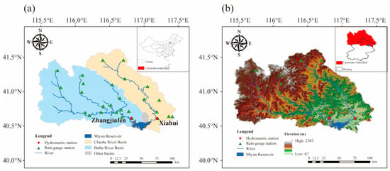
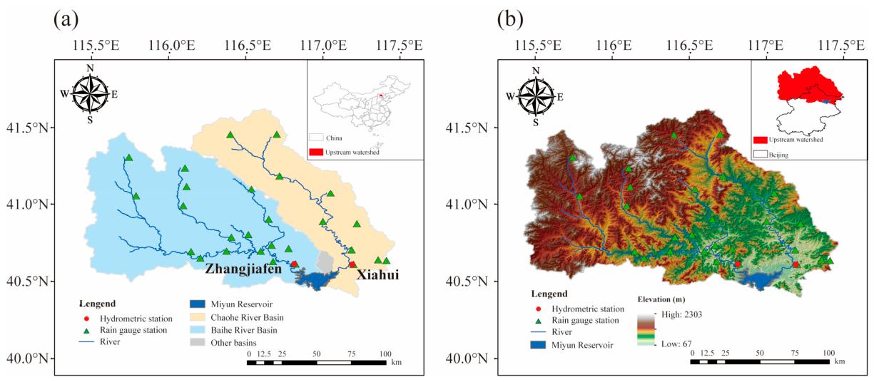
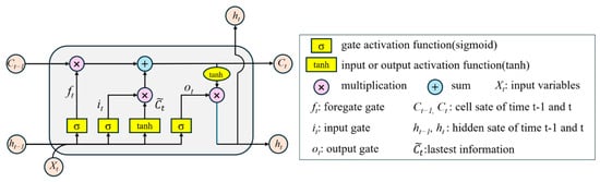
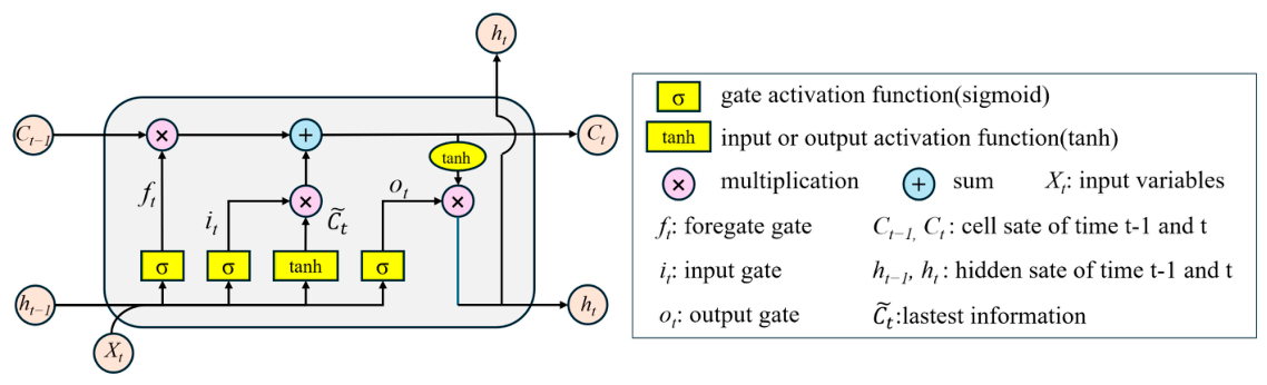
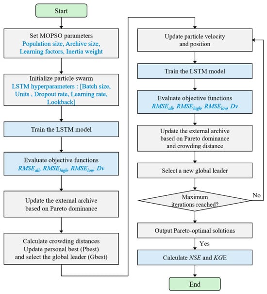
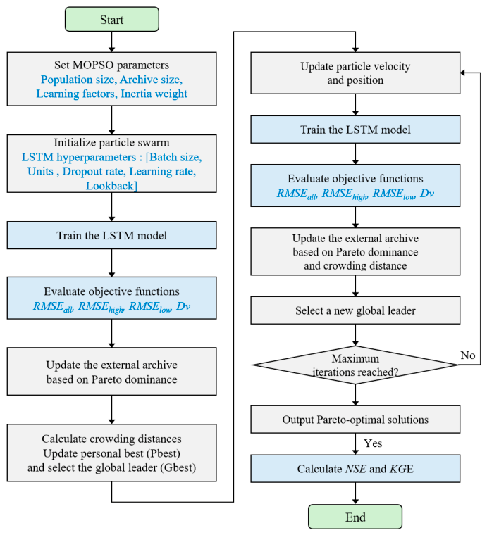
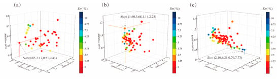
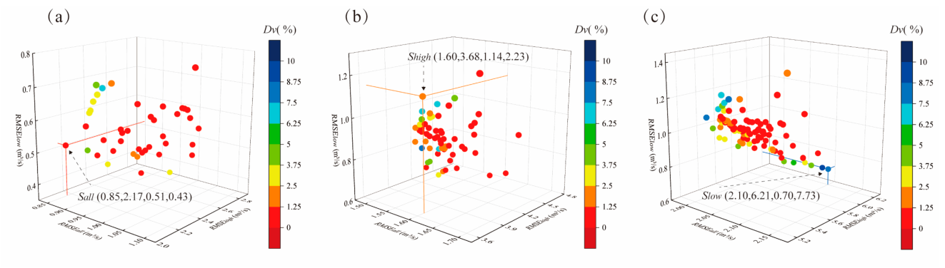
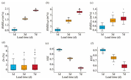
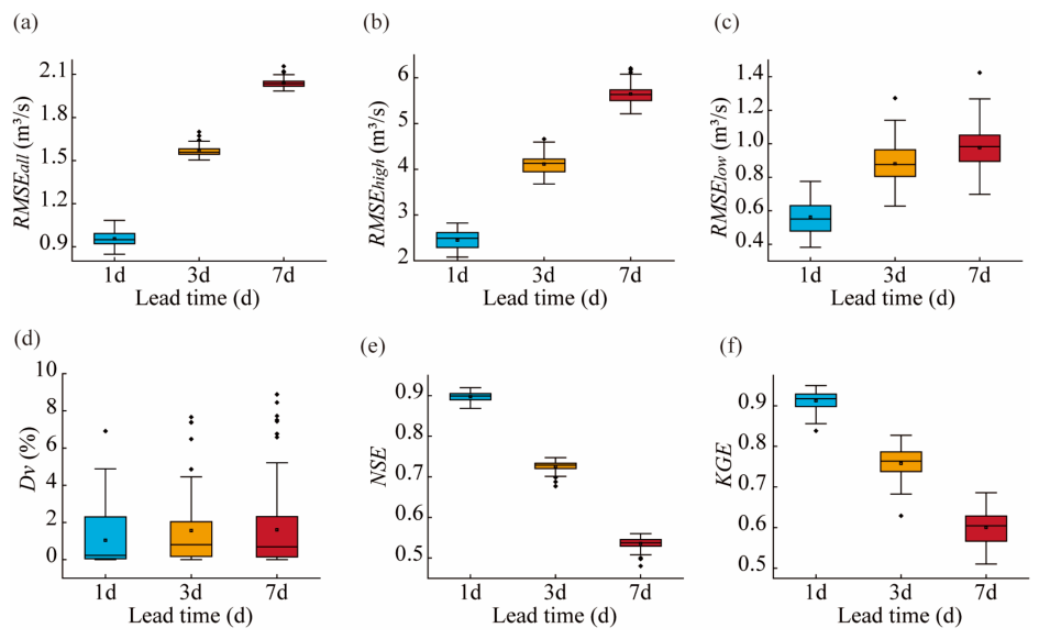
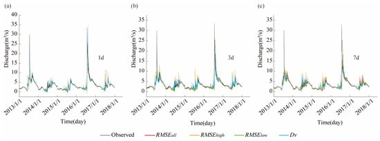
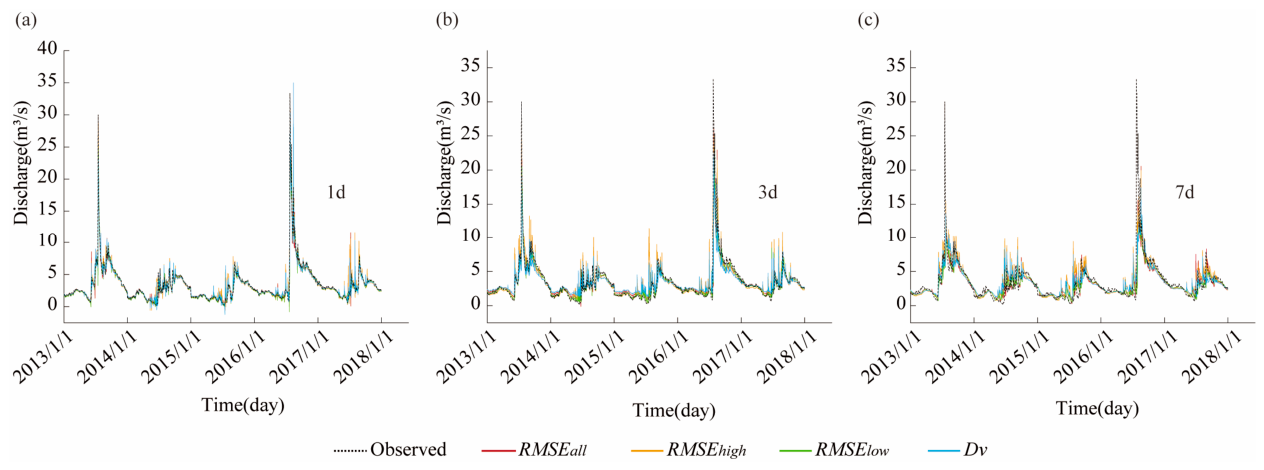
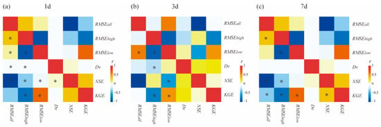
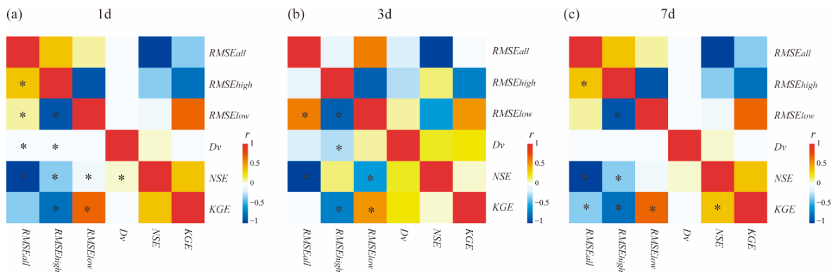
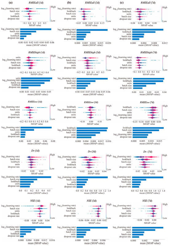
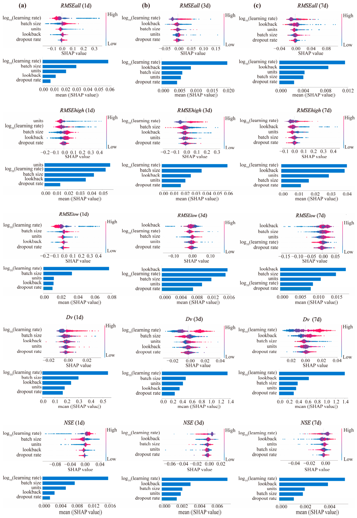
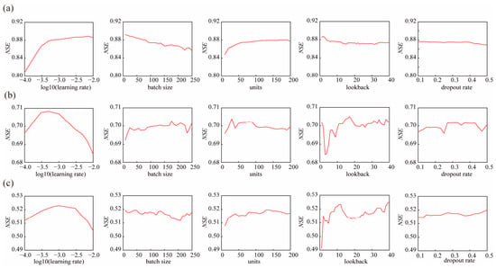
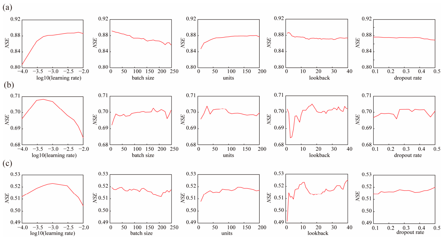
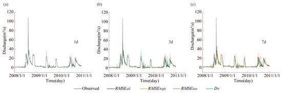
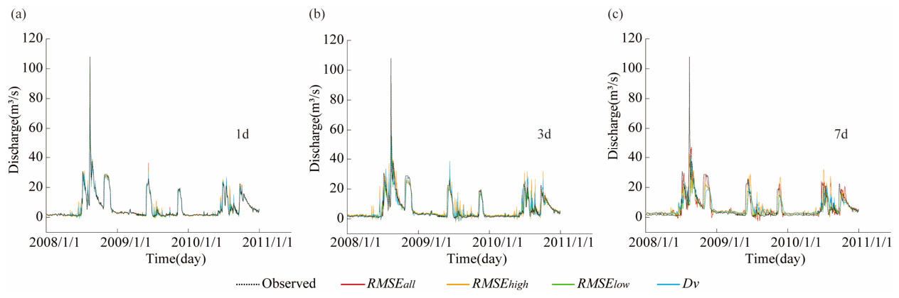

Disclaimer/Publisher’s Note: The statements, opinions and data contained in all publications are solely those of the individual author(s) and contributor(s) and not of MDPI and/or the editor(s). MDPI and/or the editor(s) disclaim responsibility for any injury to people or property resulting from any ideas, methods, instructions or products referred to in the content. |
© 2026 by the authors. Licensee MDPI, Basel, Switzerland. This article is an open access article distributed under the terms and conditions of the Creative Commons Attribution (CC BY) license.