


Abstract
Climate commitments are written for the energy system, but by restructuring the economy they also change how much water is withdrawn, and where. We soft-link, in one direction, the GTAP-E computable general equilibrium model, run for business-as-usual (BAU) and for the National Commitments (NC) of 127 countries as written (2050 caps on energy-related CO2, with no water targets), to a sector- and technology-resolved water model that allocates withdrawal to 7607 HydroBASINS level-6 basins and evaluates annual stress against Aqueduct 4.0. NC lowers 2050 withdrawal by 4.3%. Of this saving, 58% comes from cleaner production rather than a smaller economy (35–69% across sensitivity tests), and power-station cooling, 12% of demand, supplies 68%. Consumption falls by only 2.3%, mostly because the economy is smaller. The saving does not follow scarcity: stressed basins hold 59% of withdrawal but receive 45% of the saving, and 50 of 1681 stressed basins leave high stress. Under the two textbook cooling assumptions, the composition share would range from 22% to 83%; an electricity anchor checked against observed thermoelectric withdrawal narrows it. Reservoir evaporation, green hydrogen and bioenergy are not modelled. Climate policy is not a substitute for water policy.
1. Introduction
Decarbonisation is widely expected to relieve pressure on water. Thermal power plants are among the largest water users in industrialised countries, and the energy sector withdraws roughly a tenth of the world’s freshwater, mostly to cool power stations [1]. Replacing coal and gas with wind and solar, which need almost no water, therefore appears as a co-benefit of climate policy, a “win–win” for climate and water [2,3,4].
Most research on the climate–water nexus runs in the other directions: from climate change to water availability [5,6] and from water scarcity to energy supply, through the cooling constraints of thermal plants in droughts and heatwaves [7]. The arm that runs from mitigation policy to water demand has received less attention. It has mostly been studied with stylised 1.5–2 °C pathways or carbon prices [3,8,9,10] and only in a few regional cases with the actual pledges [11,12,13]. This matters because the pledges are what governments will implement, and they are silent on water. Climate plans treat water as a matter of adaptation rather than mitigation [14], and none of the national commitments assessed by [15] sets a quantified water-use target. The water outcome of the energy transition is therefore a side effect that nobody has planned, and it can work against water objectives as easily as for them [16].
Three strands of modelling each capture part of the problem.
- •
- Integrated assessment models (IAMs) with water modules. GCAM and MESSAGEix-GLOBIOM resolve some 200 basins and compute water demand endogenously from energy and land activity [17,18,19]. The rest of the economy, however, enters only as exogenous drivers or as a single macroeconomic aggregate, and the policies are usually stylised carbon prices or budgets.
- •
- CGE models with water. These capture economy-wide reallocation and trade. GTAP-W represents water as a production factor of irrigated agriculture at national or regional scale [20,21], and GTAP-BIO-W separates irrigated from rainfed cropland by agro-ecological zone [22]. Other water uses are rarely represented, and few models resolve cooling water by generation technology [23].
- •
- Plant-level cooling-water studies. These locate withdrawal precisely [24,25,26,27] but take generation scenarios as given, so the rest of the economy does not respond.
Each strand answers part of the question, but none can tell whether the water saved by climate policy comes from a cleaner economy or a smaller one, or whether it reaches the basins where water is scarce. Calls for holistic approaches that bring water, energy, emissions and economics into one frame are long-standing [23,28]. This paper puts such an approach into practice at the global scale, asking whether the climate commitments of 127 countries relieve basin water stress. It makes four contributions (C1–C4):
- •
- C1, a new model link. CGE–water studies represent water as an input to irrigated agriculture at the national or regional scale [20,21,22], and plant-level studies take the economy as given [24,25,26,27]. We couple a global CGE model (GTAP-E) with a sector- and technology-specific water model at HydroBASINS level 6, driven by the actual national commitments, so that the general-equilibrium response of every sector, including cooling water by generation technology, is evaluated across thousands of basins. Economics stays national and water stays sub-basin.
- •
- C2, a decomposition. We separate the water co-benefit of climate policy into a composition effect (cleaner production) and a scale effect (a smaller economy), for withdrawal and, in parallel, for consumption.
- •
- C3, a spatial test. We test whether the co-benefit coincides with water stress and explain why it largely does not.
- •
- C4, a methodological finding. We show that the answer to C2 swings from 22% to 83% composition with the assumed thermoelectric cooling and provide an evidence-anchored electricity water account whose modelled tier is validated against observations in 45 countries.
2. Methods
We compare two scenarios to 2050: business-as-usual (BAU; SSP2 with no commitments beyond observed policy) and National Commitments (NC; the nationally determined contributions, long-term strategies and national energy and climate plans of 127 countries, coded as 2050 caps on energy-related CO2). Both are simulated with the computable general equilibrium (CGE) model GTAP-E, calibrated to the GTAP Data Base v11 and aggregated to 128 regions and 28 sectors, including 11 power-generation technologies. The resulting sectoral output growth drives a national, sector-resolved water account calibrated to FAO AQUASTAT and to observed thermoelectric withdrawal. This demand is allocated to 7607 HydroBASINS level-6 basins with sector-specific spatial keys and compared with the available blue water of WRI Aqueduct 4.0. Basin water stress is then evaluated under three channels, each answering one question: economic (S1: what the commitments do to stress), composition (S1comp: how much of that is cleaner production rather than a smaller economy) and lower-emission world (S2: how Aqueduct’s own SSP1–2.6 projection, which combines lower demand with a milder climate, moves stress), with an availability-only variant (S2a) and a combined case (S3) as sensitivities (Figure 1). Consumption and water depletion are computed in parallel with withdrawal and stress.
Three design choices run through the framework. First, the models are soft-linked in one direction: GTAP-E determines activity, and water responds to it without feeding back into the economy. The results therefore show the water consequences of the commitments as written (a deliberately optimistic “what-if” situation to answer our research questions), not a water-constrained optimum. Second, the models exchange relative growth indices rather than absolute levels, so each component keeps its own validated base year: 2017 for GTAP-E and the national water account, and the 1979–2019 baseline for Aqueduct [29]. Third, economics stays national and water stays sub-basin. National sectoral output changes are downscaled to basins, and basin stress is never aggregated to the country, because a national stress ratio averages scarce and abundant basins and hides exactly the heterogeneity at issue [29,30]. The full chain, from GTAP output to basin channels, is scripted, runs a new GTAP scenario in about one minute, and includes regression and invariant tests that fail if results drift.
2.1. GTAP-E: The Economy Under BAU and NC
GTAP-E is the energy–environment extension of the standard multi-region, multi-sector GTAP model [31,32,33]. Markets are competitive, production has constant returns to scale, and domestic and imported goods are imperfect substitutes (Armington). GTAP-E adds a capital–energy composite with substitution between capital and energy and among fuels, and links fossil-fuel combustion to CO2 emissions, so that carbon policy is resolved inside the general equilibrium. The model is calibrated to the GTAP Data Base v11 with base year 2017 [34] and solved for a 2050 equilibrium. In economic terms, output, relative prices, trade and the allocation of labour, capital and land are determined simultaneously in every region, so that a carbon constraint on the power sector propagates through input–output linkages and trade to all other sectors. These are the general-equilibrium effects that sector-specific water studies hold fixed, and they allow the effect of one policy shock to be isolated against an otherwise identical economy [31].
Aggregation. The 128 regions and 28 sectors retain the detail that matters for water. Agriculture comprises six crop sectors (paddy rice; wheat; cereal grains; oil seeds; sugar cane and sugar beet; and other crops, which groups vegetables, fruits and nuts, plant-based fibres and crops not elsewhere classified), animal products (including fishing) and forestry. Fossil-fuel supply is represented by coal mining, crude oil, gas (including gas manufacture and distribution), and petroleum and coal products. Electricity is split into transmission and distribution and 11 generation technologies, following the GTAP-Power disaggregation [35]: nuclear, coal, gas, wind, hydro, oil and other base load, and gas, hydro, oil and solar peak load. The remaining sectors are an aggregate of 27 manufacturing industries, water services, transport and services. The technology split is what allows the water model to see the shift in cooling water: a coal plant, a nuclear plant and a wind farm produce the same electricity but withdraw very different volumes of water [2].
Figure 1.
Conceptual framework. The BAU and NC scenarios are simulated to 2050 with GTAP-E (steps 1–2). Sectoral output growth (step 3) drives a national sector water account (step 4), which is allocated to HydroBASINS level-6 basins (step 5) and compared with Aqueduct 4.0 available blue water (step 6). Basin water stress (step 7) is evaluated under three channels, each answering one question; S2a (dashed) isolates the part of S2 that is due to available water. Consumption and depletion are computed in parallel with withdrawal and stress (steps 4–7). The right-hand column shows the external data entering each step.
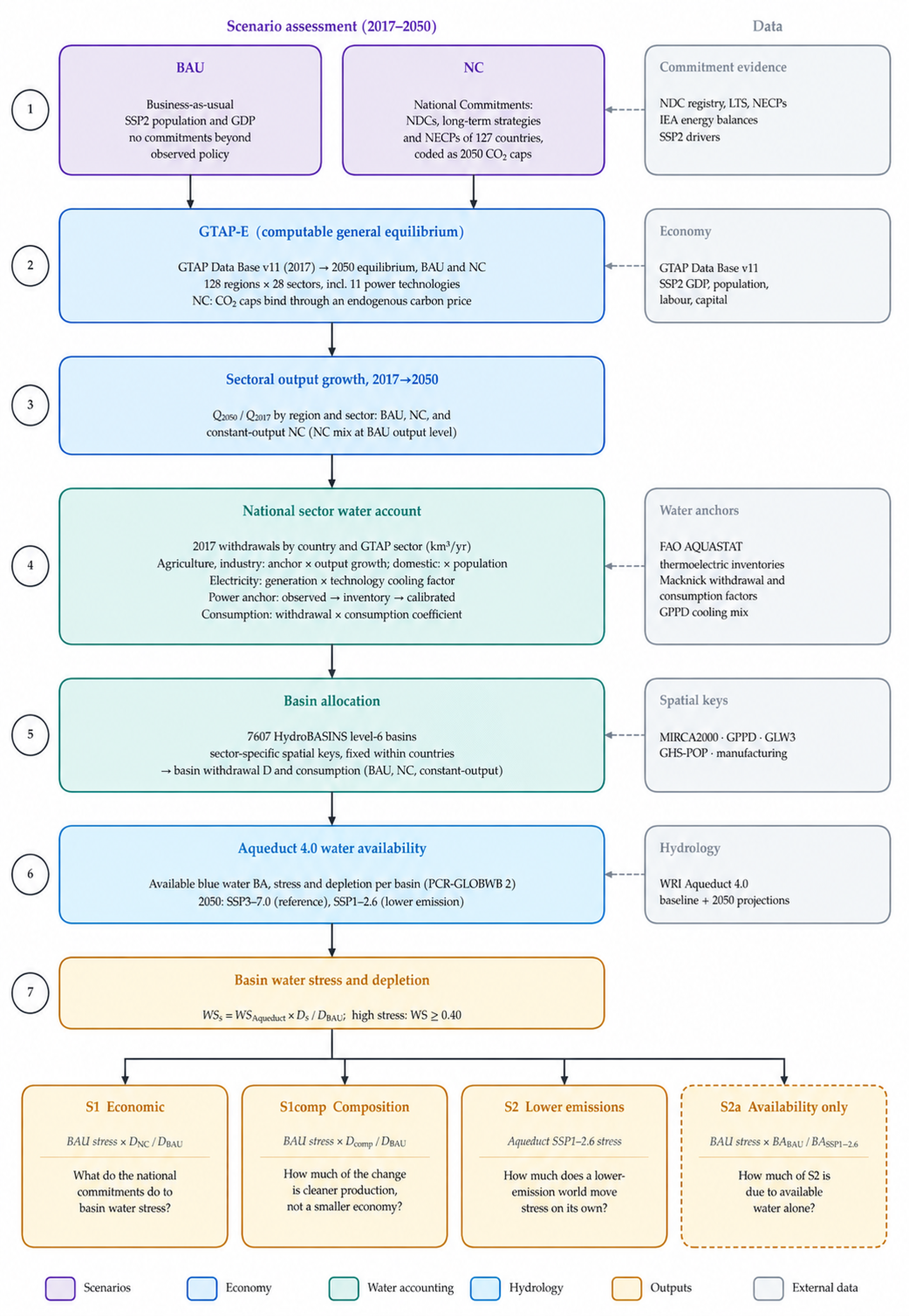
Closure and drivers. Population, GDP, labour and capital follow the SSP2 middle-of-the-road pathway in both scenarios [9,36], so the scenarios differ only in climate policy. The labour market has a full-employment closure, so sectoral labour changes are reallocations of a fixed workforce. Land endowments follow externally projected land-use trajectories for each scenario [15], which embody the land-related commitments of NC; they are treated here as exogenous inputs, like the SSP2 drivers.
The policy shock. In NC, each country’s 2050 energy-related CO2 is capped at its NC-consistent level (Section 2.3): 15,195 MtCO2 for the 127 constrained countries, 63.5% below BAU and 46% below 2017. The caps are imposed as quantity constraints, and the carbon price that makes each cap bind is determined endogenously [33]. Iran is included in both scenarios but carries no NC constraint, since its contribution was not coded with a target year and it has not ratified the Paris Agreement.
Water model inputs. The variable transferred is sectoral output (QO), the real quantity of production by region and sector, under BAU and NC in 2050 relative to 2017. GTAP-E is a system of linearised equations in percentage changes, solved in GEMPACK 12.2 with Gragg’s method and Richardson extrapolation from 2-, 4- and 6-step solutions [37]. Under large policy shocks and structural adjustment, the reported percentage change can fall below −100% in cells with very low benchmark output that contract sharply; reconstructing output levels linearly from such changes implies negative production, which has no economic meaning. This affects 176 of the 3584 region–sector cells (172 in NC and 27 in BAU), mostly coal mining, coal-fired power and gas, which together hold 0.56% of 2017 withdrawal. We keep the linear reconstruction wherever the change is above a threshold −λ, and below it use a C1-continuous exponential continuation that is strictly positive, monotone and identical to the linear rule at the threshold (Section S3.5). The central case uses λ = 50%, which leaves 93.5% of cells untouched (the rule changes 232 of 3584); λ = 30, 70 and 90%, and a bracket from full elimination of the affected activity to no contraction at all, are run as sensitivities (Table 5).
The 128 regions account for about 87% of global energy-related CO2 emissions in 2017 [15]. They exclude Russia, Ukraine, Australia and New Zealand, for which consistent input data are not currently available or are problematic; a version of the framework covering all countries is being built as these data are collected and pre-processed. The aggregation has no rest-of-world residual. Syria is excluded from the analysis as the unstable situation there leads to a solution implying negative 2050 output in 12 of 28 sectors. All totals refer to the modelled countries, not to the world; Table S1 traces the coverage from the 128 regions to the 126 countries and 7607 basins of the headline results.
2.2. WaterReqGCH: From Sectoral Output to Basin Withdrawals
Water withdrawals are computed with WaterReqGCH, a sectoral water-requirements model that estimates withdrawals as the product of an activity driver and a water-use intensity calibrated to national water accounts, and computes water stress against renewable supply following the Aqueduct methodology [15,38,39]. For this study, the model is configured for a new question and at a new resolution: its activity drivers are the 28 GTAP-E sectors, electricity is resolved by generation technology, and demand is placed in HydroBASINS level-6 basins. Withdrawal (gross abstraction) is the primary metric, because Aqueduct’s baseline water stress, SDG indicator 6.4.2 and abstraction permits are defined on it; consumption is computed in parallel (Section 2.2.5). All volumes are in km3 yr−1. The workflow has four steps (Section 2.2.1, Section 2.2.2, Section 2.2.3 and Section 2.2.4).
2.2.1. A Sector-Resolved National Water Account for 2017
National withdrawals by use category (irrigation, livestock, industry and municipal) are taken from FAO AQUASTAT [40]. Each category is allocated to the GTAP sectors that draw on it with within-category shares that sum to one, and calibrated so that the sum over sectors equals the national category total. A zero-shock scenario therefore reproduces the observed baseline exactly (validation). Irrigation is split among the six crop sectors in proportion to the irrigated harvested area of each crop in MIRCA2000 v1.1 ([41]; Section S3.1), and livestock withdrawals are distributed with the Gridded Livestock of the World [42]. GTAP-E carries no irrigated–rainfed split, so the irrigated share is absorbed into the calibrated coefficient of each crop in each country.
2.2.2. Electricity as Its Own Category, with a Tiered and Validated Anchor
AQUASTAT reports industrial withdrawal, which in most countries includes thermoelectric cooling, and only some countries report the cooling component separately. How the industrial total is split between power plants and manufacturing is therefore a modelling decision, and it decides the answer to our first research question (Section 3.4). We anchor 2017 electricity withdrawal in three tiers, using observation wherever it exists:
- •
- Tier 1, observed: AQUASTAT thermoelectric withdrawal where reported (45 countries, 284.8 km3 yr−1).
- •
- Tier 1b, national inventory: where AQUASTAT is silent but a peer-reviewed plant-level inventory exists. This applies to China, 65.2 km3 yr−1 [26], consistent with the once-through cooling floor of 49.0 km3 yr−1 reported by the Ministry of Water Resources [43].
- •
- Tier 2, modelled: for the remaining 81 countries, 2017 generation by technology is multiplied by withdrawal factors for once-through and recirculating cooling [2], blended by a country cooling mix (48.5 km3 yr−1 in total). The seawater share of the mix is measured from the coordinates of 11,626 thermal plants (4200 GW) in the Global Power Plant Database [44]: plants within 10 km of the ocean are treated as seawater-cooled and excluded from freshwater withdrawal, giving a global seawater share of 32.3%. The once-through share of freshwater cooling is 0.30 by default and was set by hand for 24 countries from information on their fleets (Table S3). Plant-level characterisation of cooling follows established practice [24,25,27].
Manufacturing then receives the AQUASTAT industrial total minus electricity, with a floor of 10% of the industrial total; where observed cooling exceeds the reported industrial total (10.1 km3 yr−1 across 23 countries), the overflow is reported rather than removed. The anchor reallocates water within industry rather than adding it: 335 km3 yr−1 moves from manufacturing to electricity, while the global account rises by only 0.26%. Electricity ends at 10.6% of the 2017 national account of 127 countries (398 km3 yr−1; 10.7% in the 126 countries of the headline results), in line with the global estimate for energy-sector withdrawal of about 400 km3 yr−1, roughly 10% of the total [1]. The 45 Tier-1 countries also provide a validation of the modelled tier. For each of them, the Tier-2 estimate was computed exactly as for a country without data and compared with the AQUASTAT value, so no observed value enters the estimate. Two pieces of outside information did enter the Tier-2 method: the once-through shares of 11 of the 45 countries were set by hand, and the mix was checked against US thermoelectric withdrawal [45]. A strict version of the test removes both (Section 3.4; Section S4).
2.2.3. From 2017 to 2050 (Routes A and B)
Agriculture, livestock, manufacturing and water services follow Route A: the 2017 withdrawal of each sector and country is scaled by that sector’s GTAP-E output growth and by a water-intensity trend τ, with τ = 1 in all runs (Equation (1)).
Ws,c,2050 = Ws,c,2017 × (Qs,c,2050/Qs,c,2017) × τ,
This holds water productivity at its 2017 level. Observed withdrawal intensities have declined over recent decades [46,47], so τ = 1 gives an upper bound on demand in both scenarios, and the same assumption applies to BAU and NC; declining intensities are tested in Table 5. Domestic withdrawal follows SSP2 population at constant per-capita use, with population growth taken from the GTAP-E BAU shock so that water and economy share one SSP2 pathway, and is therefore identical in both scenarios.
Electricity follows Route B: withdrawal is computed directly as generation multiplied by the country- and technology-specific withdrawal factor of Section 2.2.2, with generation following the GTAP-E output of each technology. Growth factors cannot be used for electricity because they are undefined for technologies that start from zero, which is exactly the case that decarbonisation creates.
2.2.4. Basin Allocation and Water Stress
National withdrawals by sector are distributed to HydroBASINS level-6 basins [48], which share their identifiers with Aqueduct 4.0, using sector-specific spatial keys:
- •
- Irrigation: MIRCA2000 irrigated areas [41];
- •
- Electricity: GPPD plant locations and capacities by technology [44], with the country’s all-plant distribution as fallback;
- •
- Livestock: GLW3 animal densities for 2010 [42];
- •
- Domestic: GHS-POP population for 2010 at 1 km [49];
- •
- Manufacturing: gridded industrial withdrawals [50].
The within-country pattern of each sector is held fixed, the standard first-order assumption in global water-use downscaling [47,50]. The allocation conserves volume, so basin totals sum exactly to national totals. Water stress is withdrawal divided by available blue water (BA), the renewable surface water and groundwater generated in or flowing into a basin minus upstream consumption, from Aqueduct 4.0 [29], which is based on PCR-GLOBWB 2 [51]. A basin is under high stress when stress ≥ 0.40 [29,52]. Because Aqueduct computes annual stress from monthly values, annual BA cannot be recovered by inverting the stress ratio, so scenario stress is obtained by scaling Aqueduct’s stress with our demand ratio (Section 2.3). The headline universe is 7607 basins in 122 countries (Table S1), after removing Aqueduct’s sentinel flags (±9999 and raw stress of exactly 1.0, which mark arid, low-use basins rather than stress levels) and excluding Syria. Analyses of withdrawal volumes further restrict this universe to basins with BAU 2050 withdrawal of at least 1 Mm3 yr−1 (7332 basins).
2.2.5. Consumption and Depletion
Consumption is computed in parallel with withdrawal, using the same national account, projection and spatial keys and a consumption-to-withdrawal coefficient for each country and sector (Section S5). Power-sector consumption uses the consumption factors of Macknick et al. [2] for the same cooling mix as withdrawal; seawater cooling consumes no freshwater. Irrigation uses each country’s ratio of irrigation water requirement to irrigation withdrawal from AQUASTAT [40], capped at one, and the median ratio of 0.35 where AQUASTAT reports no requirement. Domestic, manufacturing and livestock use fixed coefficients of 0.15, 0.10 and 0.75, within the ranges of global water-use models [46,47]. Basin consumption is evaluated against Aqueduct’s water-depletion indicator, the ratio of consumption to available water [29], scaled in the same way as stress (Equation (2)); depletion is high at 0.50 or more and extremely high at 0.75 or more. The datasets used throughout the modelling framework are summarised in Table 1.
Table 1.
Data sources.
2.3. Scenarios and Comparative Assessment
Business-as-usual. BAU is the counterfactual against which NC is measured: socio-economic development follows SSP2 and no commitments are implemented beyond those already reflected in observed data [9]. SSP2 was preferred to policy-based baselines such as the IEA Stated Policies Scenario, because these already contain part of the commitments that NC is meant to isolate [55]. In GTAP-E, BAU has no emission constraint. Energy-related CO2 of the 127 countries then grows from 28,367 MtCO2 in 2017 to 41,646 MtCO2 in 2050 (+47%) [15].
National Commitments. NC implements what countries have pledged or legislated in their NDCs (Nationally Determined Contributions), long-term strategies and, for 32 European countries, their national energy and climate plans [15]. Pledges cannot be simulated as written: they differ in reference (base year, self-declared BAU or intensity), gas and sector coverage, treatment of land use and horizon [53,56], and the interpretation of targets is the largest single source of uncertainty in pledge assessments [57]. Each commitment was therefore coded with a common template and translated with one documented procedure for all countries:
- •
- Each target is expressed as an ambition ratio: pledged economy-wide emissions divided by the emissions the country would have without the pledge. The ratio is applied to the energy-related CO2 baseline, so abatement pledged in land use or non-CO2 gases is not credited to the energy system.
- •
- Where it is unclear whether a target includes land use (LULUCF), the ratio is computed on both bases and their geometric mean is taken. Ratios are capped at one, so a target above the country’s own reference case never raises emissions above BAU [58].
- •
- Relative ambition is held constant from the target year to 2050, the simplified post-pledge extension used by the Climate Action Tracker [59].
- •
- Values come from a fixed hierarchy of evidence: official national readings first, then ratios stated in the NDC, then the reconstruction above, and finally the regional median for countries without a usable target.
- •
- Two ceilings can only lower a value. A no-backsliding ceiling, from the progression principle of Article 4.3 of the Paris Agreement [57], stops emissions rising again after a pledged peak. A neutrality ceiling applies carbon-neutrality targets, but only those anchored in law or binding national policy [60].
The resulting constraint is 15,195 MtCO2 in 2050, 63.5% below BAU. It agrees satisfactorily with pledge-based assessments by UNEP 2025 [61], the Climate Action Tracker [59] and the IEA Announced Pledges Scenario [62], given differences in scope [15,63]. In GTAP-E, NC keeps the SSP2 drivers of BAU, with land endowments set exogenously from the NC land-use trajectories reported in [15], and imposes the country caps with an endogenous carbon price (Table 2). The ambition ratio, cap and evidence level of each country are documented in the assessment of the commitments [15], and the coding was also used, in part, in peer-reviewed assessments of Greece’s climate-neutrality plan [16] and of 35 European national energy and climate plans [64]; Section S2 summarises the coding template.
Table 2.
Definition of the BAU and NC scenarios in each model.
The commitments were also coded for water. None sets a quantified, enforceable water-use target at national scale [15], in line with the treatment of water as a matter of adaptation rather than mitigation in climate plans [14]. No water target is therefore imposed in either scenario: water use differs between BAU and NC only through the activity drivers. This is the design of the study, not an omission, so we can measure the water outcome that climate policy produces without being asked to.
Scenario stress is evaluated through three channels, kept deliberately separate so that each answers one question (Table 3). In S1 and S1comp, the Aqueduct 2050 stress of each basin b is scaled by the ratio of scenario to BAU withdrawal:
where WSAq,2050 is Aqueduct’s 2050 stress under SSP3–7.0 and D our basin withdrawal. Aqueduct builds annual stress from monthly values, so it is not the ratio of annual withdrawal to annual available blue water: in Aqueduct’s own data, the annual ratio is a median 0.64 of the published stress. Any indicator built from monthly ratios scales with withdrawal when withdrawal changes by the same factor in every month, so Equation (2) is exact under two assumptions: the scenario changes a basin’s withdrawal in the same proportion in every month, and available water is Aqueduct’s SSP3–7.0 BA in both scenarios. S1 and S1comp therefore use the same supply in both scenarios, and every difference in stress between BAU and NC comes from demand. The first assumption is tested with monthly irrigation profiles (Section 3.5). The second ignores the rise in downstream BA when NC lowers upstream consumption, which the consumption account bounds (Section 3.7).
WSb,s = WSbAq,2050 × Db,s/Db,BAU, s ∈ {NC, comp},
Table 3.
The stress channels. D is basin withdrawal, BA available blue water and WSBAU Aqueduct’s 2050 stress under SSP3–7.0; subscripts denote the scenario (comp = constant-output NC). High stress is WS ≥ 0.40. The depletion channel (Section 3.7) applies the S1 construction to consumption and Aqueduct’s depletion indicator.
Aqueduct 4.0 publishes future stress for SSP1–2.6, SSP3–7.0 and SSP5–8.5 only, with no SSP2 variant, and we use SSP3–7.0, Aqueduct’s business-as-usual, as the BAU stress level. The Aqueduct scenario sets only the level of stress in each basin. The NC effect is our demand ratio, which comes entirely from the SSP2-based GTAP-E runs, so what depends on the Aqueduct scenario is how many basins lie near the threshold. For the same reason, the water-intensity trend τ does not enter the BAU stress map, and a uniform τ cancels in the demand ratio. Section 3.5 repeats the threshold test on Aqueduct’s 1979–2019 baseline, its SSP5–8.5 projection, the SSP3–7.0 stress rebased to our own SSP2 demand and the annual ratio of our demand to Aqueduct’s BA.
S2 is Aqueduct’s own 2050 stress under SSP1–2.6. It combines milder climate projections with Aqueduct’s SSP1 demand, so it describes a lower-emission world rather than hydrology alone, and we call it the lower-emission channel. To separate the two, the availability-only variant S2a keeps Aqueduct’s BAU stress and changes only available water, WSBAU × BABAU/BASSP1–2.6; because Aqueduct’s BA nets out upstream consumption, S2a still carries some SSP1 demand. S3, which combines the S1 demand change with the S2 change in availability, partly double-counts and is reported in Table 6 as a sensitivity only.
The NC–BAU change in total withdrawal is split into a scale and a composition component, following the scale–composition–technique decomposition of environmental change [65,66]. The composition counterfactual keeps the NC mix of sectors and power technologies in each region but restores BAU output: NC output of every sector is multiplied by sc = Σs Qs,c,2017 xs,c,BAU/Σs Qs,c,2017 xs,c,NC, where Qs,c,2017 is the 2017 benchmark output value of sector s in region c and x its 2050 activity index, so that sc is the ratio of two fixed-base (Laspeyres) volume aggregates at 2017 prices. Domestic withdrawal is population-driven and is not rescaled. The composition effect is the change from BAU to this constant-output counterfactual, and the scale effect is the remainder. Because τ = 1 and the withdrawal factors are the same in both scenarios, the technique effect is zero by construction, so composition here measures cleaner production: a shift in what is produced and with which technology.
The actual pledges, rather than stylised pathways, drive a general-equilibrium economy whose power sector is resolved by technology and placed at real plant locations. The water anchor that decides the result is validated against observed thermoelectric withdrawal. For robustness, the results are tested against the following, one assumption at a time and on the same GTAP-E solution:
- •
- The two cooling bounds, recirculating everywhere and once-through everywhere, and a third case in which all new capacity is cooled with towers on freshwater;
- •
- A China bracket of 49–109 km3 yr−1, from the MWR once-through floor to the uncorrected modelled value, and a fully modelled anchor, with both evidence tiers switched off;
- •
- The seawater rule (5 and 20 km instead of 10 km), the siting of new capacity and an alternative irrigation key from WaterGAP 2.2d [54];
- •
- Declining water intensities (τ < 1) at two rates within the ranges of past and projected water use [46,47], and the λ grid of 30, 50, 70 and 90% with the bracket for cells below −100%;
- •
- A water-side test of the GTAP-E substitution elasticities, the stress level against which the threshold is tested, and a decomposition at national rather than basin level.
New capacity is generation above the 2017 level of each country and technology. In the cooling test, it is cooled with towers on freshwater; in the siting tests, it is placed with the country’s whole thermal fleet, or only in basins not under high stress in BAU, instead of at the existing plants of its technology. GTAP-E could not be re-solved for this study, so the elasticities are tested on the water side: a higher substitution elasticity meets the same caps with a larger shift in the technology mix and a smaller loss of output, and a lower one does the reverse. We therefore scale the NC–BAU change in the power-technology mix by 1.5 and in sectoral output by 0.5, and the reverse. This is a stylised test, not a re-solve (Section S6).
3. Results
3.1. The Economy Under the National Commitments
The caps reshape fossil supply and the power sector and leave the rest of the economy almost unchanged (Figure 2). Total 2050 output of the 128 regions is 2.0% lower under NC than under BAU. Fossil-fuel supply contracts most: coal mining by 79%, gas by 47%, petroleum and coal products by 17% and crude oil by 13%. Within electricity, output shifts from fossil to low-carbon technologies: coal base load falls by 46.5% and gas by 23–24%, while wind rises by 48%, nuclear by 39% and hydro base load by 37%. Transmission and distribution, a proxy for total electricity volume, falls by 19%. Solar: peak-load solar output rises by only 1.7%. This modest additional effect partly reflects the GTAP-E-Power structure, in which solar is represented only within the peak-load nest and therefore does not directly substitute for coal base-load generation, where much of the fossil-fuel contraction occurs. Moreover, the NC scenario imposes CO2 quantity constraints rather than technology-specific renewable deployment targets, allowing the model to meet the emissions cap through the endogenous combination of lower fossil generation, and greater use of alternative low-carbon technologies such as wind, hydro and nuclear. Solar output already expands substantially from 2017 to 2050 (by 65.9% under BAU and 68.8% under NC), so the additional effect of the commitments is comparatively small (+1.7%). Outside energy, changes are small: crop sectors fall by 0.8–3.2%, manufacturing industries by 2.2% and transport by 4.0%, while services are unchanged (+0.1%). The endogenous carbon price required to meet the NC emissions constraints, GTAP-E’s real carbon tax rate (the nominal rate deflated by the model’s income-price deflator), varies substantially across countries. Median values, in constant 2017 USD per tonne of CO2, are highest in Africa (336.4), followed by the Americas (272.5), Europe (237.7) and Asia (175.5), reflecting differences in the stringency of national constraints and in the sectoral and technological options available for abatement. The distribution of costs follows the energy trade: welfare losses concentrate in fossil-fuel exporters, most importers gain, and labour is reallocated towards electricity, energy-intensive industries and transport [15].
Figure 2.
Change in 2050 output under NC relative to BAU (%), by GTAP region and sector group: 100 × (NC/BAU − 1), with output valued at 2017 prices; colours are clipped at ±100%. The median across regions is given above each panel. Hatched: countries not modelled; grey: no output in BAU. Robinson projection.
3.2. How Much Water, and in Which Sectors
In the headline basins, 2050 withdrawal under BAU is 5730 km3 yr−1, 59% above 2017, with water productivity held constant. NC lowers it by 247 km3 yr−1, or 4.30% (Table 4). The saving is dominated by one sector. Electricity accounts for 12.5% of BAU demand but 68% of the saving: power-sector withdrawal falls by 23.4% (−167 km3 yr−1). Irrigation, which is 71% of demand, falls by only 1.5% and provides 25% of the saving. Manufacturing falls by 4.5% (6% of the saving), and domestic withdrawal, which follows population (+12% from 2017), is unchanged by construction.
Table 4.
Withdrawal in 2050 by category, headline basins: 7607 basins in 122 countries (km3 yr−1). Constant output: NC sector and technology mix at BAU output level (S1comp). In the national account of 127 countries, 2017 electricity withdrawal is 398 km3 yr−1 (Table S1).
Inside the power sector, the transition exchanges one cooling water for another. Withdrawal for coal base-load plants halves, from 332 to 165 km3 yr−1, and gas falls by about 40%. Withdrawal for nuclear plants rises by 35%, from 182 to 245 km3 yr−1. The growth of nuclear therefore gives back more than a third of the water saved on coal. Wind and solar withdraw essentially nothing, and hydropower is assigned no withdrawal, although its reservoirs evaporate water that no withdrawal account records.
Nationally, the United States, China and India provide 63% of the saving (−10.4%, −7.2% and −3.1% of their withdrawal). Countries whose water use is dominated by irrigation barely move: Pakistan and Egypt fall by 0.3% and 0.8%, and Iraq and Uzbekistan by 1.4% and 1.8%. Withdrawal rises in 28 of the 126 countries. Among them, Iran, which carries no NC constraint, rises by 2.1%, consistent with production relocating towards unconstrained regions. Results for every country and category are in Supplementary Data S1.
3.3. Cleaner or Smaller? The Decomposition
Holding total output at its BAU level, NC still lowers withdrawal by 2.50%. Of the 4.30% saving, 58.1% is therefore a composition effect, cleaner production, and 41.9% a scale effect, a smaller economy (Figure 3a). The composition effect comes entirely from electricity (−22.1% at constant output) and manufacturing (−2.7%). At constant output, irrigation and livestock withdrawals rise slightly (+0.6% and +0.8%), because agriculture’s share of a rescaled economy grows. The result is robust (Table 5): the composition share ranges from 56.3% to 62.4% across the China bracket, is 58.0–58.1% across λ = 30–90%, is 57.1% when the decomposition is done at national rather than basin level, and is 58.1% with a fully modelled anchor. The evidence-based and the fully modelled anchors thus agree to within 0.1 percentage points. Across the seawater rule, the siting of new capacity, the irrigation key, declining water intensities and the treatment of GTAP cells below −100%, the composition share stays between 56.7% and 62.7%. Two assumptions move it more: the cooling of new capacity (Section 3.4) and, in the stylised water-side test, the GTAP-E substitution elasticities, which give 43.6% and 69.3%.
Figure 3.
Scale and composition of the NC water saving under the three cooling anchors and with all new capacity on cooling towers, for the same GTAP-E run. (a) Share of the 2050 NC–BAU withdrawal saving due to composition (cleaner production at constant output) and scale (smaller economy); the total change is given under each label, and the whisker on the central case is the China bracket (Table 5). (b) Electricity’s share of the 2017 withdrawal account of the 126 headline countries in each case (the new-capacity case shares the account of the tiered anchor), against the published range of 10–15% (shaded).
Table 5.
Cooling anchor comparison and robustness (same GTAP-E solution; λ = 50% and τ = 1 unless stated). Electricity 2017 and its share refer to the 126 headline countries. S1: basins newly stressed/relieved, of 1681 stressed in BAU. The stress-level tests are in Table S9.
3.4. Why the Cooling Anchor Decides the Answer
The decomposition depends on how much water is assigned to power plants in 2017. With the same GTAP run, the same basins and everything else unchanged, assuming recirculating cooling everywhere gives 22% composition and 78% scale, and assuming once-through cooling everywhere gives 83% and 17% (Figure 3a; Table 5). The mechanism is the size of the electricity account (Figure 3b). Recirculating cooling puts power at 1.4% of 2017 withdrawal (54 km3 yr−1) and files the rest of the cooling water under manufacturing, which is almost pure scale. Once-through cooling puts power at 35.2% (1734 km3 yr−1). Only the tiered anchor, at 10.7%, lies within the published range of 10–15%. The total saving changes with the anchor as well, from −2.36% to −10.21%.
How new capacity is cooled matters as much. The central case gives new capacity the cooling mix of each country’s 2017 fleet. If instead all generation above 2017 levels is cooled with towers on freshwater, the nuclear expansion adds almost no withdrawal (+4 instead of +64 km3 yr−1), but the coal and gas capacity that BAU would build and NC avoids would also have withdrawn less. The saving then falls to 2.71%, the composition share falls to 35.0%, and S1 relieves 38 basins instead of 50 (Table 5; Table S8). Power-sector consumption rises (37.8 instead of 33.1 km3 yr−1 in BAU), because cooling towers withdraw less but consume more. This is the largest sensitivity we found, and we report it as a third bound (Figure 3a).
The observations choose among the three (Figure 4). For each of the 45 countries that report thermoelectric withdrawal, the modelled tier was applied exactly as for a country without data, so no observed value enters the estimate. The calibrated cooling mix then has a median modelled-to-observed ratio of 1.05, and its total (268 km3 yr−1) is close to the observed 285 km3 yr−1. Recirculating everywhere underestimates by a factor of eight (median ratio 0.12; total 21 km3 yr−1). Once-through everywhere overestimates by a factor of four (median ratio 4.38; total 754 km3 yr−1), and would require 1215 km3 yr−1 more industrial water than national statistics report. Country-level scatter remains wide (17 of 45 countries are within a factor of two of observation; for example, France at 1.95 and the Netherlands at 0.07), which is why observed values take precedence over the model wherever they exist.
Figure 4.
Validation of the modelled tier of the electricity water anchor. Modelled (Tier-2 method; no observed value used) against observed (AQUASTAT) 2017 thermoelectric withdrawal in the 45 reporting countries, under (a) recirculating cooling everywhere, (b) the calibrated cooling mix and (c) once-through cooling everywhere. Log–log axes; the line is 1:1 and the shaded band is within a factor of two. In (b), one country with zero modelled withdrawal cannot be shown on log axes. A strict version of (b), without hand-set once-through shares, is in Table S4.
The calibrated mix is not entirely independent of observations: the once-through shares of 11 of the 45 countries were set by hand, and the mix was checked against US thermoelectric withdrawal [45]. In a strict version of the test, with the default once-through share for all 45 countries and no US check, the median ratio is 0.84 and the total 173 km3 yr−1, 39% below observation; 91 of the 112 km3 yr−1 shortfall is in the United States, and without it the median is 0.85 and the total 21% low (Table S4). The strict test is less accurate in total, but within a factor of 1.2 of observation at the median, against factors of four to eight for the textbook assumptions. China, for which AQUASTAT reports no thermoelectric value, enters the account through its plant-level inventory; the modelled tier would overestimate it by a factor of 1.67, which is why the China bracket is tested in Table 5.
3.5. Where the Saving Lands: Basins
Across basins, the NC change in withdrawal is small, and it is concentrated in a few regions (Figure 5). The median basin loses 1.6% of its 2050 withdrawal, and withdrawal rises in 1238 of 7332 basins. The largest cuts, above 5%, lie in the eastern United States, western and central Europe and northern China, where thermal power plants are concentrated. The outlined high-stress basins of the Indus, the Ganges, the Nile, the Tigris–Euphrates and northern Mexico change little, and Iran stands out with increases throughout.
The threshold test gives the same picture (Table 6). Of the 1681 basins under high stress in BAU, S1 relieves 50 and pushes seven further basins over the threshold. Forty-five of the 50 relieved basins were already between 0.40 and 0.50, so they cross the threshold without materially changing their scarcity. Of the 1055 basins under extremely high stress (≥0.80), 36 leave that class. In 293 of the stressed basins, withdrawal rises.
Table 6.
Basins crossing the high-stress threshold, by channel and cooling case (newly stressed/relieved), of 1681 basins stressed in BAU. S2 (100/170, of 1638 stressed basins on its valid universe) and S2a (47/79) use no demand data from this study and are the same in every case. S3 is a sensitivity only.
Measured continuously, the change is small almost everywhere. NC closes less than 1% of the gap between BAU stress and the threshold in 170 stressed basins, 1–5% in 492 and 5–25% in 516 (Section S8). The median change in stress grows with stress, from −0.003 in basins at 0.1–0.2 to −0.038 in basins above 0.8, but in relative terms it is about −2% in every class above 0.1. The count of relieved basins depends little on the stress level used for BAU. On Aqueduct’s 1979–2019 baseline, its SSP5–8.5 projection, its SSP3–7.0 stress rebased to our SSP2 demand and the annual ratio of our demand to available water, S1 relieves 48–73 basins, and 94.6–97.0% of the basins stressed in BAU remain stressed under NC (Table S9). Nor does it depend on the annual scaling: with irrigation distributed over the months by MIRCA2000 monthly irrigated areas, the median change in the month of peak withdrawal in stressed basins (−2.2%) equals the annual change, and scaling stress by it relieves the same 50 basins (Section S9).
Figure 5.
Change in 2050 withdrawal under NC relative to BAU, by HydroBASINS level-6 basin (%). Outlined: basins under high stress in BAU (WS ≥ 0.40). Grey: basins outside the modelled regions (Russia, Ukraine, Australia, New Zealand), flagged by Aqueduct as arid and low-use, or with BAU withdrawal below 1 Mm3 yr−1. Robinson projection.
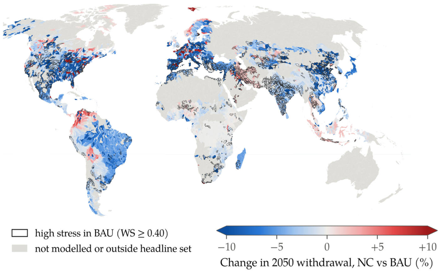
Stressed basins do not receive a smaller relative cut: their median withdrawal falls by 2.2%, against 1.5% in other basins. The mismatch is in volume (Figure 6). Stressed basins hold 59% of BAU withdrawal but only 39% of power-sector withdrawal, and so receive only 45% of the saving. Weighted by demand, electricity is 8.2% of withdrawal in stressed basins and 18.7% in the others, and its share falls steadily with stress, from 22.0% in basins below 0.1 to 5.9% in basins above 0.8 (Figure 6a). Basin by basin, the relation is flat: the unweighted mean share is 8.0% in stressed basins and 7.9% elsewhere. The rank correlation is weakly positive (Spearman ρ = 0.27), because 71% of the basins below 0.1 host no power plant at all (Figure 6a). The saving is made where power stations are a large part of demand; where water is scarcest, the pressure is irrigation, which the commitments leave almost unchanged.
Figure 6.
The spatial mismatch. (a) Electricity’s share of basin withdrawal in BAU 2050 against basin water stress (7332 basins with BAU withdrawal ≥ 1 Mm3 yr−1; log scale; dashed line: high-stress threshold; basins without power plants, with a share of zero, are jittered). Lines give the mean and the demand-weighted share in each Aqueduct stress class. (b) Share of BAU withdrawal, of power-sector withdrawal and of the NC saving located in high-stress basins.
Where new capacity is built shapes this mismatch but does not remove it. Of the gross reduction in power-sector withdrawal under NC, 77% is capacity that BAU would build and NC avoids, and only 23% lies within the 2017 fleet size, so the location of avoided and added capacity is an assumption. Placing new capacity with each country’s whole thermal fleet, instead of at the existing plants of its technology, lowers the stressed share of the saving from 45% to 42%. Keeping new capacity out of basins under high stress in BAU lowers it to 26%, with 36 basins relieved, because the expansion that NC avoids would then have been outside stressed basins as well (Table S8).
3.6. The Commitments Against a Lower-Emission World
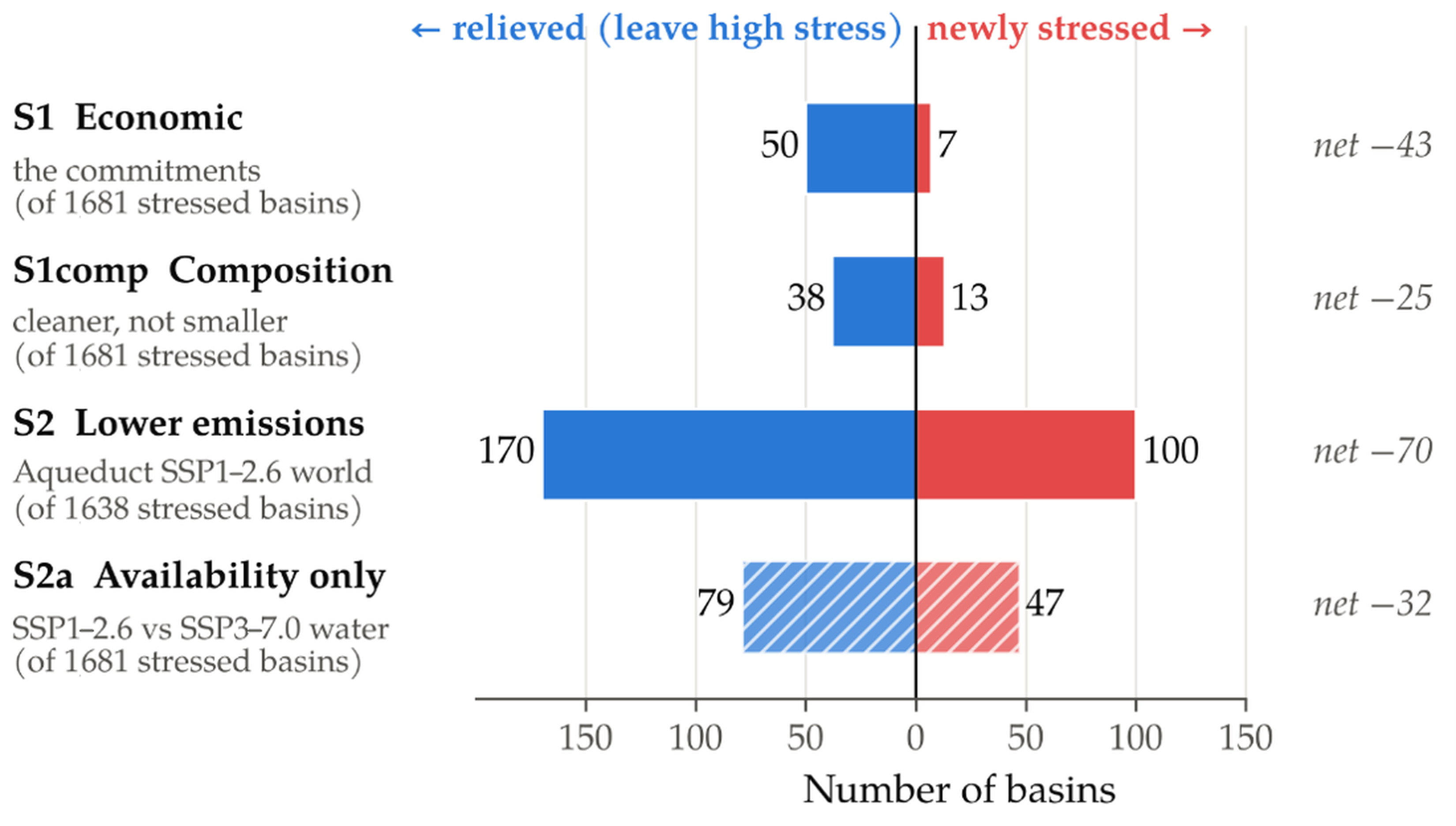
The lower-emission channel moves more basins than the economic one (Figure 7). Under Aqueduct’s SSP1–2.6 projection for 2050 (S2), 170 basins leave high stress and 100 enter it, on its own valid universe of 1638 stressed basins, a net change of −70 against −43 for S1. The composition channel alone relieves 38 basins and stresses 13 (net −25), confirming that cleaner production by itself moves few basins across the threshold. Holding Aqueduct’s demand at BAU and changing only available water (S2a) relieves 79 basins and stresses 47 (net −32), so at most about half of the S2 effect comes from available water and the rest from the SSP1 demand that S2 embeds. S2 and S2a are identical in every cooling case, as they must be, since they use no demand data from this study; the combined case S3 is given in Table 6 as a sensitivity only.
The channels overlap at the margin: 23 of the 50 basins relieved by S1 are also relieved by S2, which confirms that both act mainly on basins close to the threshold. Because S2 embeds Aqueduct’s SSP1 demand as well as milder climate, it measures a lower-emission world rather than hydrology alone.
Figure 7.
Basins crossing the high-stress threshold (WS ≥ 0.40) under the three channels and the availability-only variant S2a (hatched), central case. Left: basins stressed in BAU that fall below the threshold (relieved). Right: basins pushed over it (newly stressed). In parentheses: basins stressed in BAU on each channel’s valid universe.
3.7. Consumption and Depletion
Consumption tells a smaller and less technological story. In the headline basins, 2050 consumption under BAU is 1764 km3 yr−1, 31% of withdrawal, and NC lowers it by 2.3% (40 km3 yr−1). Irrigation is 88% of consumption in the headline countries. Power-plant cooling consumes only 4.5% of what it withdraws, because once-through cooling returns almost all of its water, so it supplies 24% of the consumption saving, against 68% of the withdrawal saving; irrigation supplies 69%. At constant output, consumption falls by only 0.27%, so 12% of the consumption saving is composition and 88% scale (Table S6). Measured as consumption, the water co-benefit of the commitments is therefore mostly the by-product of a smaller economy.
The spatial result holds for consumption. Stressed basins hold 63% of BAU consumption and receive 55% of the consumption saving; consumption falls by 2.0% in stressed basins and by 2.9% elsewhere. Against Aqueduct’s depletion indicator, 18 of the 902 basins under high depletion in BAU (≥0.50) leave that class and five enter it; of the 631 basins under extremely high depletion (≥0.75), 13 leave and three enter. Because NC lowers consumption by only about 2%, the rise in downstream available water that Equation (2) ignores is at most about 2% of upstream consumption, a second-order correction to stress (Section S5).
4. Discussion
The analysis simulates the commitments as written; it does not optimise them. It can say what the pledges do to water withdrawal and stress, and through which sectors, technologies and places. It cannot say what the least-water or least-cost route to the same emissions would be, because neither water nor cost enters the choice of the energy mix. The primary indicator is annual withdrawal pressure on renewable blue water, with consumption and depletion reported beside it (Section 3.7). It is not water quality, environmental flow or seasonal scarcity, each of which can tell a different story about the same withdrawals. Within these bounds, the results support four findings.
4.1. Climate Policy Is a Power-Sector Water Policy, by Accident
Sixty-eight per cent of the water saved under the commitments comes from power-station cooling, which is 12% of demand. The rest of the economy barely changes its water use, and irrigation, 71% of demand, falls by 1.5%. The saving is real, and more than half of it is technological: at constant output, the NC economy still withdraws 2.5% less water than BAU. This matters because, in an economy-wide model, lower water use could simply reflect lower activity. Here, most of the gain comes from what is produced and how, not from producing less. This holds for withdrawal, not for consumption: consumption falls by 2.3%, and only 12% of that is composition, because once-through cooling withdraws far more than it consumes, while irrigation, which dominates consumption, barely changes (Section 3.7). The composition share also depends on how new capacity is cooled (Section 3.4). However, none of it was designed. The commitments were written for carbon, and their water benefit follows the geography of thermal power, existing and avoided, not the geography of scarcity.
4.2. The Co-Benefit Is Real but Spatially Blind
The saving lands in the Ohio and Mississippi basins, the Rhine and Danube, and the North China Plain, where thermal fleets are concentrated. It hardly reaches the Indus, the Ganges, the Nile or the Tigris–Euphrates, where stress is driven by irrigation. Stressed basins hold 59% of withdrawal but 39% of power-sector withdrawal and receive 45% of the saving. Of 1681 stressed basins, 50 cross below the threshold and 45 of them were within 0.1 of it. Where a basin crosses, its scarcity has hardly changed: it moved from just above an indicator threshold to just below it. The mismatch holds for consumption, of which stressed basins hold 63% and receive 55% of the saving. Alternative siting of new capacity strengthens rather than removes it, because relief in stressed basins depends on retiring or forgoing plants that would otherwise be there (Section 3.5). The lower-emission channel moves more basins in both directions than the economic one, but it combines lower demand with a milder climate, and at most about half of it comes from available water (Section 3.6).
4.3. The Energy Transition Redistributes Water Rather than Simply Saving It
Inside the power sector, the commitments exchange one cooling water for another. Coal-plant withdrawal halves, but nuclear withdrawal rises by 35%, returning 38% of the water saved on coal. How much it returns depends on how new plants are cooled: with cooling towers, the nuclear expansion adds almost no withdrawal but more consumption (Section 3.4). Hydro base-load output expands by more than a third; its reservoirs evaporate water that no withdrawal account records [67], and evaporation from new reservoirs is one reason why water consumption can rise while withdrawal falls in decarbonisation scenarios [13]. Green hydrogen, which the commitments introduce in 44 countries [15], and irrigated bioenergy are not represented in the GTAP sectors used here. Both would add demand, often in sunny, dry regions [68,69]. The water dividend of decarbonisation is therefore not a uniform reduction but a redistribution: from coal to nuclear and hydro, from inland rivers to coasts, and potentially from withdrawal to consumption.
4.4. The Hidden Assumption
The size and the nature of the water co-benefit depend on a choice that most integrated models leave implicit: how much of national industrial water is cooling water. With the same economy and the same basins, the composition share of the saving ranges from 22% to 83% between the two textbook cooling assumptions, and the total saving from 2.4% to 10.2%. Only the tiered anchor matches the observed thermoelectric withdrawal of the 45 reporting countries and fits within national industrial accounts. The cooling of new capacity is a second hidden assumption: if all of it uses cooling towers, the composition share falls to 35%. Two lessons follow for modelling. Couplings of economic and water models should validate their electricity water anchor against reported data, state that they did, and state how new capacity is cooled. And AQUASTAT reports thermoelectric withdrawal separately for only 45 countries, so better reporting would do as much to improve these estimates as better models.
4.5. Comparison with Previous Work
The direction of the results agrees with multi-model studies of deep decarbonisation, which find net water co-benefits from phasing out coal but pressures from nuclear, carbon capture and bioenergy [3,9]. It also agrees with regional IAM studies, in which the water effects of decarbonisation differ strongly between provinces and basins depending on the sectoral mix [12,13]. Three things differ here. The scenario is the set of pledges rather than a target-consistent optimum. The economy is in general equilibrium, which makes it possible to separate composition from scale. Additionally, the spatial test is made at HydroBASINS level 6, about 16,000 units globally, rather than at a few hundred basins, which is where the mismatch between power plants and irrigated scarcity becomes visible. The results also confirm, at higher resolution, the qualitative finding of the global assessment of the commitments that withdrawals fall in most hotspots but too little to change the map of water stress [15], and they identify the mechanism behind it. Similar unintended consequences of climate plans for water have been shown at the national scale [16].
4.6. Limitations
Linking a global economy to thousands of basins requires simplifying assumptions. Each assumption below was needed to make the analysis possible at this scale, and each was either tested or chosen so that its bias runs in a known direction.
- •
- Withdrawal intensities are held at 2017 levels (τ = 1), which overstates 2050 demand in both scenarios and makes demand volumes an upper bound. τ does not enter the BAU stress map, which is Aqueduct’s, and a uniform τ cancels in the demand ratio. With intensities declining at rates within the range of past and projected water use, BAU growth to 2050 falls from 59% to 30–44%, while the NC saving (4.6–4.9%) and the composition share (60–63%) change little (Table 5).
- •
- The once-through share of freshwater cooling is set by hand for 24 countries, and China’s anchor rests on a single plant-level inventory (2014, freshwater scope inferred). Both are tested: the modelled tier is only 12% of power water, the strict validation without hand-set shares is within a factor of 1.2 of observation at the median, and the China bracket of 49–109 km3 moves the composition share between 56.3% and 62.4%. The cooling and siting of new capacity are assumptions as well; cooling towers on all new capacity lower the composition share to 35% (Section 3.4).
- •
- Irrigation follows GTAP-E crop output rather than land-use projections. Crop output changes little between the scenarios (−0.8% to −3.2%), so this choice cannot reverse the result; a land-use-driven sensitivity is left for further work. The irrigation key matters little: WaterGAP irrigation withdrawal instead of MIRCA2000 area gives a composition share of 58.3%.
- •
- Consumption is estimated with fixed consumption-to-withdrawal coefficients outside the power sector and irrigation (Section 2.2.5), and reservoir evaporation is not included, so the consumption account is less certain than the withdrawal account.
- •
- Stress is annual. Equation (2) assumes that NC changes withdrawal in the same proportion in every month; a check with monthly irrigation profiles finds the peak-month change equal to the annual change in stressed basins, because irrigation dominates them in every month (Section 3.5). Monthly hydrology and environmental flows are not modelled.
- •
- The 128 GTAP regions omit Russia, Ukraine, Australia and New Zealand, for which consistent input data are not currently available or are problematic; Syria is excluded, and Aqueduct’s sentinel basins are removed. Totals therefore refer to the modelled countries, and some arid basins cannot be assessed. Russia and Australia hold large thermal fleets, so global totals would be larger; a version of the framework covering all countries is being built.
- •
- S2 uses Aqueduct’s SSP1–2.6 stress, which embeds SSP1 demand as well as milder climate, so it is a lower-emission world rather than hydrology alone; the availability-only variant S2a still carries some SSP1 demand through Aqueduct’s BA. Neither is additive with S1 (hence S3 is a sensitivity only).
- •
- GTAP-E could not be re-solved for this study. The cells whose change falls below −100% hold 0.56% of 2017 withdrawal, and treating them as fully eliminated or as not contracting moves the composition share by less than one percentage point. The substitution elasticities were tested only on the water side, by scaling the NC–BAU change in the technology mix and in output; this stylised test gives a composition share of 44–69% and should be confirmed by a systematic sensitivity analysis in GTAP-E.
- •
- Green hydrogen and irrigated bioenergy are not separate sectors in the GTAP aggregation, and evaporation from new reservoirs is not a withdrawal. All three would add water use under NC, so the net water benefit reported here is likely an upper bound.
The robustness tests (Table 5) cover the most consequential of these choices: the cooling of the existing fleet and of new capacity, the electricity anchor, the seawater rule, the siting of new capacity, the irrigation key, water intensity, the treatment of GTAP cells below −100%, the elasticities and the spatial level of the decomposition. Apart from the textbook cooling bounds, the composition share stays between 35% and 69%: a substantial part of the saving is cleaner production in every test, and more than half in all but two. The spatial mismatch holds in every test: stressed basins receive less of the saving than their share of withdrawal, and at most 54 of the 1681 stressed basins are relieved. Several limitations are shared by most climate–water assessments: implicit cooling-water anchoring, unaccounted reservoir evaporation and new water users, annual indicators and incomplete country coverage. They point to the next steps. Siting-constrained scenarios inside GTAP-E would test whether placing new generation away from stressed basins can move the dividend to where it is needed. A basin-level optimisation with a shadow price of water under the carbon constraint would show where water limits make the commitments costlier to meet, and a two-way link, in which binding basins feed back into GTAP-E, would close the loop. Monthly hydrology, land-use-driven irrigation and explicit hydrogen and bioenergy demand would test the results against the dimensions of scarcity that annual indicators miss.
5. Conclusions and Policy Implications
The climate commitments of 127 countries, simulated as written and without water targets, lower 2050 water withdrawal by 4.3%, and 58% of the saving is cleaner production rather than the by-product of a smaller economy. The saving comes mainly from power-station cooling, and it lands where power stations are, not where water is scarce: stressed basins hold 59% of withdrawal but receive 45% of the saving, and 50 of 1681 stressed basins leave high stress, most of them from just above the threshold. Measured as consumption, the saving is smaller (2.3%) and mostly a scale effect. In irrigation-dominated basins, the commitments leave water stress essentially where BAU puts it.
These conclusions concern annual withdrawal and consumption under a one-way link, and they rest on assumptions that we could test only in part. The composition share depends on how power plants are cooled, from 22% to 83% between the textbook assumptions and 35% if all new capacity uses cooling towers, and on substitution elasticities that GTAP-E could not re-solve. The spatial mismatch, in contrast, holds in every test, for withdrawal and for consumption, and alternative siting of new capacity strengthens it.
The following implications are inferences from these results; they were not themselves modelled.
- •
- Water co-benefits of climate plans need a basin-level check. A national saving coexists here with unchanged stress in the basins that matter, so national totals say little about scarcity. NDCs, long-term strategies and national energy and climate plans could report the water their measures withdraw and consume, by basin, alongside land and investment [15,16].
- •
- Siting is the lever that could move the dividend. Most of the power-sector saving is expansion that the commitments avoid, so where new capacity is built and old capacity retires decides where water is saved. Screening new thermal and nuclear capacity against basin stress, prioritising retirements in stressed freshwater-cooled basins and favouring seawater, dry or hybrid cooling where basins are stressed follow from the cooling and siting tests (Section 3.4 and Section 3.5) [27].
- •
- Irrigation needs its own policy. Irrigation is 71% of 2050 withdrawal and 88% of consumption and barely moves under the commitments, so relief in the most stressed basins would have to come from water policy itself: allocation, efficiency programmes that cap rather than relabel the water they save, and dietary and yield levers [15].
- •
- The transition redistributes water. Planners could expect less abstraction by inland coal plants and more by nuclear plants, reservoirs and, outside our model, green hydrogen and irrigated bioenergy, often in different basins and seasons [13,67,68,69]. River basin plans, such as those for 2028–2033 under the EU Water Framework Directive, could include the water demand implied by national energy and climate plans as an explicit pressure scenario.
- •
- Better data would matter as much as better models. Only 45 countries report thermoelectric withdrawal to AQUASTAT, and the missing number decides what integrated models conclude about composition. Plant-level reporting of cooling withdrawal and consumption would serve climate and water planning alike.
Climate policy is not a substitute for water policy. Linking the two, basin by basin, would turn an accidental co-benefit into a deliberate one.
Supplementary Materials
The following supporting information can be downloaded at: https://www.mdpi.com/article/10.3390/hydrology13110309/s1, Supplementary Materials (Sections S1–S10, Table S1–S12) and Supplementary Data S1 (country-level inputs and results, Excel workbook). These suplementary materials provide additional details on country and basin coverage, the coding of National Commitments, water model methodology, electricity withdrawal calibration and validation, water consumption and depletion, robustness and sensitivity analyses, alternative water stress scenarios, seasonality, and code and data availability. All references cited in the Supplementary Materials are also included in the main manuscript reference list.
Author Contributions
Conceptualization, A.A. and P.K.; methodology, A.A., E.C. and I.A.; software, A.A., E.C. and I.A.; validation, A.A., E.C., I.A. and P.K.; formal analysis, A.A., E.C. and I.A.; data curation, A.A., E.C. and I.A.; visualization, A.A. and I.A.; writing—original draft preparation, A.A., E.C. and I.A.; writing—review and editing, A.A., E.C., I.A. and P.K.; supervision, A.A. and P.K. All authors have read and agreed to the published version of the manuscript.
Funding
This research received no external funding.
Institutional Review Board Statement
Not applicable.
Informed Consent Statement
Not applicable.
Data Availability Statement
The code of the water model and of every analysis in this paper, the derived spatial keys, the cooling and anchor tables, the GTAP-E output indices that drive the water model and all model outputs are archived on Zenodo [39] https://zenodo.org/records/24013827 (accessed on 16 November 2026). Country-level inputs and results are in Supplementary Data S1. The input datasets are available in the UNFCCC NDC Registry (https://unfccc.int/NDCREG) (accessed on 16 November 2026); SSP Scenario Database, IIASA (https://data.ece.iiasa.ac.at/ssp/, accessed on 16 November 2026); FAO AQUASTAT (https://www.fao.org/aquastat/en/, accessed on 16 November 2026); Aqueduct 4.0 Current and Future Global Maps Data, World Resources Institute (https://www.wri.org/data/aqueduct-global-maps-40-data, accessed on 16 November 2026); HydroBASINS v1c, level 6 (https://www.hydrosheds.org/products/hydrobasins, accessed on 16 November 2026); Global Power Plant Database v1.3.0, World Resources Institute (https://datasets.wri.org/dataset/globalpowerplantdatabase, accessed on 16 November 2026); MIRCA2000 v1.1 (https://www.uni-frankfurt.de/45218023/MIRCA, accessed on 16 November 2026); Gridded Livestock of the World v3 (GLW3, 2010), Harvard Dataverse (https://doi.org/10.7910/DVN/GIVQ75 and the companion records listed in https://doi.org/10.1038/sdata.2018.227, accessed on 16 November 2026); GHS-POP R2023A, European Commission Joint Research Centre (https://data.jrc.ec.europa.eu/dataset/2ff68a52-5b5b-4a22-8f40-c41da8332cfe, accessed on 16 November 2026); Global gridded monthly sectoral water use dataset v2 (https://doi.org/10.5281/zenodo.1209296, accessed on 16 November 2026); water withdrawal factors for power generation from [2]; China thermoelectric water withdrawal from [26]. The GTAP Data Base v11, including GTAP-Power, used to calibrate GTAP-E is available under licence from the Center for Global Trade Analysis, Purdue University (https://www.gtap.agecon.purdue.edu/databases/v11/, accessed on 16 November 2026) and cannot be redistributed.
Acknowledgments
During the preparation of this manuscript/study, the authors used AI for the purposes of language and syntax editing and clarity. The authors have reviewed and edited the output and take full responsibility for the content of this publication.
Conflicts of Interest
The authors declare no conflicts of interest.
Abbreviations
The following abbreviations are used in this manuscript: BA, available blue water; BAU, business-as-usual; CGE, computable general equilibrium; GPPD, Global Power Plant Database; GTAP, Global Trade Analysis Project; GTAP-E, energy–environment version of the GTAP model; IAM, integrated assessment model; LTS, long-term strategy; NC, National Commitments; NDC, nationally determined contribution; NECP, national energy and climate plan; SSP, Shared Socioeconomic Pathway; WS, water stress.
References
- International Energy Agency. World Energy Outlook 2016; IEA: Paris, France, 2016. [Google Scholar]
- Macknick, J.; Newmark, R.; Heath, G.; Hallett, K.C. Operational water consumption and withdrawal factors for electricity generating technologies: A review of existing literature. Environ. Res. Lett. 2012, 7, 045802. [Google Scholar] [CrossRef] [Scilit]
- Mouratiadou, I.; Biewald, A.; Pehl, M.; Bonsch, M.; Baumstark, L.; Klein, D.; Popp, A.; Luderer, G.; Kriegler, E. The impact of climate change mitigation on water demand for energy and food: An integrated analysis based on the Shared Socioeconomic Pathways. Environ. Sci. Policy 2016, 64, 48–58. [Google Scholar] [CrossRef] [Scilit]
- Jin, Y.; Behrens, P.; Tukker, A.; Scherer, L. Water use of electricity technologies: A global meta-analysis. Renew. Sustain. Energy Rev. 2019, 115, 109391. [Google Scholar] [CrossRef] [Scilit]
- Schewe, J.; Heinke, J.; Gerten, D.; Haddeland, I.; Arnell, N.W.; Clark, D.B.; Dankers, R.; Eisner, S.; Fekete, B.M.; Colón-González, F.J.; et al. Multimodel assessment of water scarcity under climate change. Proc. Natl. Acad. Sci. USA 2014, 111, 3245–3250. [Google Scholar] [CrossRef] [Scilit]
- Graham, N.T.; Hejazi, M.I.; Chen, M.; Davies, E.G.R.; Edmonds, J.A.; Kim, S.H.; Turner, S.W.D.; Li, X.; Vernon, C.R.; Calvin, K.; et al. Humans drive future water scarcity changes across all Shared Socioeconomic Pathways. Environ. Res. Lett. 2020, 15, 014007. [Google Scholar] [CrossRef] [Scilit]
- van Vliet, M.T.H.; Wiberg, D.; Leduc, S.; Riahi, K. Power-generation system vulnerability and adaptation to changes in climate and water resources. Nat. Clim. Change 2016, 6, 375–380. [Google Scholar] [CrossRef] [Scilit]
- Kyle, P.; Davies, E.G.R.; Dooley, J.J.; Smith, S.J.; Clarke, L.E.; Edmonds, J.A.; Hejazi, M. Influence of climate change mitigation technology on global demands of water for electricity generation. Int. J. Greenh. Gas. Control 2013, 13, 112–123. [Google Scholar] [CrossRef] [Scilit]
- Fricko, O.; Havlik, P.; Rogelj, J.; Klimont, Z.; Gusti, M.; Johnson, N.; Kolp, P.; Strubegger, M.; Valin, H.; Amann, M.; et al. The marker quantification of the Shared Socioeconomic Pathway 2: A middle-of-the-road scenario for the 21st century. Glob. Environ. Change 2017, 42, 251–267. [Google Scholar] [CrossRef] [Scilit]
- Mouratiadou, I.; Bevione, M.; Bijl, D.L.; Drouet, L.; Hejazi, M.; Mima, S.; Pehl, M.; Luderer, G. Water demand for electricity in deep decarbonisation scenarios: A multi-model assessment. Clim. Change 2018, 147, 91–106. [Google Scholar] [CrossRef] [Scilit]
- Santos da Silva, S.R.; Miralles-Wilhelm, F.; Muñoz-Castillo, R.; Clarke, L.E.; Braun, C.J.; Delgado, A.; Edmonds, J.A.; Hejazi, M.; Horing, J.; Horowitz, R.; et al. The Paris pledges and the energy-water-land nexus in Latin America: Exploring implications of greenhouse gas emission reductions. PLoS ONE 2019, 14, e0215013. [Google Scholar] [CrossRef] [Scilit]
- Licandeo, F.; Flores, F.; Feijoo, F. Assessing the impacts of economy-wide emissions policies in the water, energy, and land systems considering water scarcity scenarios. Appl. Energy 2023, 342, 121115. [Google Scholar] [CrossRef] [Scilit]
- Younis, O.; Davies, E.G.R.; Chiappori, D.V.; Binsted, M.; Siddiqui, M.-S.; Arbuckle, E.J.; Macaluso, N. Exploring water use pathways under deep decarbonization scenarios in Canada at subnational scales using GCAM-Canada. J. Environ. Manag. 2025, 391, 126416. [Google Scholar] [CrossRef] [Scilit]
- UNESCO; UN-Water. The United Nations World Water Development Report 2020: Water and Climate Change; UNESCO: Paris, France, 2020. [Google Scholar]
- Koundouri, P.; Alamanos, A.; Arampatzidis, I.; Palatnik, R.R.; Maili, E.; Lanzett, H.; Mavrogenis, S.; McLannahan, M. Integrated Systems Modelling and Assessment of the Global National Commitments; UN SDSN Global Climate Hub: Athens, Greece, 2026. [Google Scholar]
- Koundouri, P.; Alamanos, A.; Arampatzidis, I.; Devves, S.; Dellis, K.; Deranian, C. Assessing national climate-neutrality plans through a modelling nexus lens: The case of Greece. npj Clim. Action 2025, 4, 113. [Google Scholar] [CrossRef] [Scilit]
- Hejazi, M.; Edmonds, J.; Clarke, L.; Kyle, P.; Davies, E.; Chaturvedi, V.; Wise, M.; Patel, P.; Eom, J.; Calvin, K.; et al. Long-term global water projections using six socioeconomic scenarios in an integrated assessment modeling framework. Technol. Forecast. Soc. Change 2014, 81, 205–226. [Google Scholar] [CrossRef] [Scilit]
- Kim, S.H.; Hejazi, M.; Liu, L.; Calvin, K.; Clarke, L.; Edmonds, J.; Kyle, P.; Patel, P.; Wise, M.; Davies, E. Balancing global water availability and use at basin scale in an integrated assessment model. Clim. Change 2016, 136, 217–231. [Google Scholar] [CrossRef] [Scilit]
- Awais, M.; Vinca, A.; Byers, E.; Frank, S.; Fricko, O.; Boere, E.; Burek, P.; Poblete Cazenave, M.; Kishimoto, P.N.; Mastrucci, A.; et al. MESSAGEix-GLOBIOM nexus module: Integrating water sector and climate impacts. Geosci. Model Dev. 2024, 17, 2447–2469. [Google Scholar] [CrossRef] [Scilit]
- Berrittella, M.; Hoekstra, A.Y.; Rehdanz, K.; Roson, R.; Tol, R.S.J. The economic impact of restricted water supply: A computable general equilibrium analysis. Water Res. 2007, 41, 1799–1813. [Google Scholar] [CrossRef] [Scilit]
- Calzadilla, A.; Rehdanz, K.; Tol, R.S.J. Water scarcity and the impact of improved irrigation management: A computable general equilibrium analysis. Agric. Econ. 2011, 42, 305–323. [Google Scholar] [CrossRef] [Scilit]
- Taheripour, F.; Hertel, T.W.; Liu, J. The role of irrigation in determining the global land use impacts of biofuels. Energy Sustain. Soc. 2013, 3, 4. [Google Scholar] [CrossRef] [Scilit]
- Bardazzi, E.; Bosello, F. Critical reflections on water-energy-food nexus in computable general equilibrium models: A systematic literature review. Environ. Model. Softw. 2021, 145, 105201. [Google Scholar] [CrossRef] [Scilit]
- Vassolo, S.; Döll, P. Global-scale gridded estimates of thermoelectric power and manufacturing water use. Water Resour. Res. 2005, 41, W04010. [Google Scholar] [CrossRef] [Scilit]
- Raptis, C.E.; van Vliet, M.T.H.; Pfister, S. Global thermal pollution of rivers from thermoelectric power plants. Environ. Res. Lett. 2016, 11, 104011. [Google Scholar] [CrossRef] [Scilit]
- Liao, X.; Hall, J.W.; Eyre, N. Water use in China’s thermoelectric power sector. Glob. Environ. Change 2016, 41, 142–152. [Google Scholar] [CrossRef] [Scilit]
- Lohrmann, A.; Farfan, J.; Caldera, U.; Lohrmann, C.; Breyer, C. Global scenarios for significant water use reduction in thermal power plants based on cooling water demand estimation using satellite imagery. Nat. Energy 2019, 4, 1040–1048. [Google Scholar] [CrossRef] [Scilit]
- Koundouri, P.; Alamanos, A.; Plataniotis, A.; Stavridis, C.; Perifanos, K.; Devves, S. Assessing the sustainability of the European Green Deal and its interlinkages with the SDGs. npj Clim. Action 2024, 3, 23. [Google Scholar] [CrossRef] [Scilit]
- Kuzma, S.; Bierkens, M.F.P.; Lakshman, S.; Luo, T.; Saccoccia, L.; Sutanudjaja, E.H.; Van Beek, R. Aqueduct 4.0: Updated Decision-Relevant Global Water Risk Indicators; Technical Note; World Resources Institute: Washington, DC, USA, 2023. [Google Scholar] [CrossRef] [Scilit]
- Vörösmarty, C.J.; Green, P.; Salisbury, J.; Lammers, R.B. Global water resources: Vulnerability from climate change and population growth. Science 2000, 289, 284–288. [Google Scholar] [CrossRef] [Scilit]
- Hertel, T.W. (Ed.) Global Trade Analysis: Modeling and Applications; Cambridge University Press: Cambridge, UK, 1997. [Google Scholar]
- Burniaux, J.-M.; Truong, T.P. GTAP-E: An Energy-Environmental Version of the GTAP Model; GTAP Technical Paper No. 16; Center for Global Trade Analysis; Purdue University: West Lafayette, IN, USA, 2002. [Google Scholar]
- McDougall, R.; Golub, A. GTAP-E: A Revised Energy-Environmental Version of the GTAP Model; GTAP Research Memorandum No. 15; Center for Global Trade Analysis; Purdue University: West Lafayette, IN, USA, 2007. [Google Scholar]
- Aguiar, A.; Chepeliev, M.; Corong, E.; van der Mensbrugghe, D. The Global Trade Analysis Project (GTAP) Data Base: Version 11. J. Glob. Econ. Anal. 2022, 7, 1–37. [Google Scholar] [CrossRef] [Scilit]
- Peters, J.C. The GTAP-Power Data Base: Disaggregating the electricity sector in the GTAP Data Base. J. Glob. Econ. Anal. 2016, 1, 209–250. [Google Scholar] [CrossRef] [Scilit]
- Riahi, K.; van Vuuren, D.P.; Kriegler, E.; Edmonds, J.; O’Neill, B.C.; Fujimori, S.; Bauer, N.; Calvin, K.; Dellink, R.; Fricko, O.; et al. The Shared Socioeconomic Pathways and their energy, land use, and greenhouse gas emissions implications: An overview. Glob. Environ. Change 2017, 42, 153–168. [Google Scholar] [CrossRef] [Scilit]
- Harrison, W.J.; Pearson, K.R. Computing solutions for large general equilibrium models using GEMPACK. Comput. Econ. 1996, 9, 83–127. [Google Scholar] [CrossRef] [Scilit]
- Alamanos, A.; Koundouri, P. Estimating the Water Requirements per Sector in Europe. In Proceedings of the 5th IAHR Young Professionals Congress, Online, 27–29 November 2024; Available online: https://www.iahr.org/index/detail/1576 (accessed on 10 October 2026).
- Alamanos, A.; Challah, E.; Arampatzidis, I.; Koundouri, P. WaterReqGCH Coupled to GTAP-E: Code, Derived Inputs and Results for “Does Decarbonisation Relieve Water Scarcity?”; Zenodo: Geneva, Switzerland, 2026; Available online: https://zenodo.org/records/24013827.
- FAO. AQUASTAT—FAO’s Global Information System on Water and Agriculture. Available online: https://www.fao.org/aquastat/en/ (accessed on 10 October 2026).
- Portmann, F.T.; Siebert, S.; Döll, P. MIRCA2000—Global monthly irrigated and rainfed crop areas around the year 2000: A new high-resolution data set for agricultural and hydrological modeling. Glob. Biogeochem. Cycles 2010, 24, GB1011. [Google Scholar] [CrossRef] [Scilit]
- Gilbert, M.; Nicolas, G.; Cinardi, G.; Van Boeckel, T.P.; Vanwambeke, S.O.; Wint, G.R.W.; Robinson, T.P. Global distribution data for cattle, buffaloes, horses, sheep, goats, pigs, chickens and ducks in 2010. Sci. Data 2018, 5, 180227. [Google Scholar] [CrossRef] [Scilit]
- Ministry of Water Resources of the People’s Republic of China. China Water Resources Bulletin. Available online: http://www.mwr.gov.cn/english/ (accessed on 10 October 2026).
- Byers, L.; Friedrich, J.; Hennig, R.; Kressig, A.; Li, X.; Malaguzzi Valeri, L.; McCormick, C. A Global Database of Power Plants; World Resources Institute: Washington, DC, USA; Available online: https://datasets.wri.org/dataset/globalpowerplantdatabase (accessed on 10 October 2026).
- Dieter, C.A.; Maupin, M.A.; Caldwell, R.R.; Harris, M.A.; Ivahnenko, T.I.; Lovelace, J.K.; Barber, N.L.; Linsey, K.S. Estimated Use of Water in the United States in 2015; U.S. Geological Survey Circular 1441; USGS: Reston, VA, USA, 2018. [Google Scholar] [CrossRef] [Scilit]
- Flörke, M.; Kynast, E.; Bärlund, I.; Eisner, S.; Wimmer, F.; Alcamo, J. Domestic and industrial water uses of the past 60 years as a mirror of socio-economic development: A global simulation study. Glob. Environ. Change 2013, 23, 144–156. [Google Scholar] [CrossRef] [Scilit]
- Wada, Y.; Flörke, M.; Hanasaki, N.; Eisner, S.; Fischer, G.; Tramberend, S.; Satoh, Y.; van Vliet, M.T.H.; Yillia, P.; Ringler, C.; et al. Modeling global water use for the 21st century: The Water Futures and Solutions (WFaS) initiative and its approaches. Geosci. Model Dev. 2016, 9, 175–222. [Google Scholar] [CrossRef] [Scilit]
- Lehner, B.; Grill, G. Global river hydrography and network routing: Baseline data and new approaches to study the world’s large river systems. Hydrol. Process. 2013, 27, 2171–2186. [Google Scholar] [CrossRef] [Scilit]
- Schiavina, M.; Freire, S.; Carioli, A.; MacManus, K. GHS-POP R2023A—GHS Population Grid Multitemporal (1975–2030); European Commission, Joint Research Centre: Ispra, Italy, 2023. [Google Scholar] [CrossRef]
- Huang, Z.; Hejazi, M.; Li, X.; Tang, Q.; Vernon, C.; Leng, G.; Liu, Y.; Döll, P.; Eisner, S.; Gerten, D.; et al. Reconstruction of global gridded monthly sectoral water withdrawals for 1971–2010 and analysis of their spatiotemporal patterns. Hydrol. Earth Syst. Sci. 2018, 22, 2117–2133. [Google Scholar] [CrossRef] [Scilit]
- Sutanudjaja, E.H.; van Beek, R.; Wanders, N.; Wada, Y.; Bosmans, J.H.C.; Drost, N.; van der Ent, R.J.; de Graaf, I.E.M.; Hoch, J.M.; de Jong, K.; et al. PCR-GLOBWB 2: A 5 arcmin global hydrological and water resources model. Geosci. Model Dev. 2018, 11, 2429–2453. [Google Scholar] [CrossRef] [Scilit]
- Alcamo, J.; Döll, P.; Henrichs, T.; Kaspar, F.; Lehner, B.; Rösch, T.; Siebert, S. Global estimates of water withdrawals and availability under current and future “business-as-usual” conditions. Hydrol. Sci. J. 2003, 48, 339–348. [Google Scholar] [CrossRef] [Scilit]
- United Nations Framework Convention on Climate Change. Nationally Determined Contributions Under the Paris Agreement: Synthesis Report by the Secretariat; FCCC/PA/CMA/2025/8; UNFCCC: Bonn, Germany, 2025. [Google Scholar]
- Müller Schmied, H.; Cáceres, D.; Eisner, S.; Flörke, M.; Herbert, C.; Niemann, C.; Peiris, T.A.; Popat, E.; Portmann, F.T.; Reinecke, R.; et al. The global water resources and use model WaterGAP v2.2d: Model description and evaluation. Geosci. Model Dev. 2021, 14, 1037–1079. [Google Scholar] [CrossRef] [Scilit]
- International Energy Agency. World Energy Outlook 2025; IEA: Paris, France, 2025. [Google Scholar]
- Pauw, W.P.; Klein, R.J.T.; Mbeva, K.; Dzebo, A.; Cassanmagnago, D.; Rudloff, A. Beyond headline mitigation numbers: We need more transparent and comparable NDCs to achieve the Paris Agreement on climate change. Clim. Change 2018, 147, 23–29. [Google Scholar] [CrossRef] [Scilit]
- Rogelj, J.; Fricko, O.; Meinshausen, M.; Krey, V.; Zilliacus, J.J.J.; Riahi, K. Understanding the origin of Paris Agreement emission uncertainties. Nat. Commun. 2017, 8, 15748. [Google Scholar] [CrossRef] [Scilit]
- Meinshausen, M.; Lewis, J.; McGlade, C.; Gütschow, J.; Nicholls, Z.; Burdon, R.; Cozzi, L.; Hackmann, B. Realization of Paris Agreement pledges may limit warming just below 2 °C. Nature 2022, 604, 304–309. [Google Scholar] [CrossRef] [Scilit]
- Climate Action Tracker. Available online: https://climateactiontracker.org/ (accessed on 10 October 2026).
- Hale, T.; Smith, S.M.; Black, R.; Cullen, K.; Fay, B.; Lang, J.; Mahmood, S. Assessing the rapidly-emerging landscape of net zero targets. Clim. Policy 2022, 22, 18–29. [Google Scholar] [CrossRef] [Scilit]
- United Nations Environment Programme. Emissions Gap Report 2025: Off Target. Continued Collective Inaction Puts Global Temperature Goal at Risk; UNEP: Nairobi, Kenya, 2025. [Google Scholar]
- International Energy Agency. World Energy Outlook 2024; IEA: Paris, France, 2024. [Google Scholar]
- den Elzen, M.G.J.; Dafnomilis, I.; Forsell, N.; Fragkos, P.; Fragkiadakis, K.; Höhne, N.; Kuramochi, T.; Nascimento, L.; Roelfsema, M.; van Soest, H.; et al. Updated nationally determined contributions collectively raise ambition levels but need strengthening further to keep Paris goals within reach. Mitig. Adapt. Strateg. Glob. Change 2022, 27, 33. [Google Scholar] [CrossRef] [Scilit]
- Koundouri, P.; Alamanos, A.; Arampatzidis, I.; Devves, S.; Pliakou, T.; Deranian, C. A simulation-driven assessment of 35 European National Energy and Climate Plans. Resources 2026, 15, 141. [Google Scholar] [CrossRef] [Scilit]
- Grossman, G.M.; Krueger, A.B. Environmental Impacts of a North American Free Trade Agreement; NBER Working Paper No. 3914; National Bureau of Economic Research: Cambridge, MA, USA, 1991. [Google Scholar] [CrossRef] [Scilit]
- Grossman, G.M.; Krueger, A.B. Economic growth and the environment. Q. J. Econ. 1995, 110, 353–377. [Google Scholar] [CrossRef] [Scilit]
- Mekonnen, M.M.; Hoekstra, A.Y. The blue water footprint of electricity from hydropower. Hydrol. Earth Syst. Sci. 2012, 16, 179–187. [Google Scholar] [CrossRef] [Scilit]
- Beswick, R.R.; Oliveira, A.M.; Yan, Y. Does the green hydrogen economy have a water problem? ACS Energy Lett. 2021, 6, 3167–3169. [Google Scholar] [CrossRef] [Scilit]
- Stenzel, F.; Greve, P.; Lucht, W.; Tramberend, S.; Wada, Y.; Gerten, D. Irrigation of biomass plantations may globally increase water stress more than climate change. Nat. Commun. 2021, 12, 1512. [Google Scholar] [CrossRef] [Scilit]
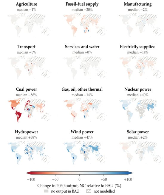
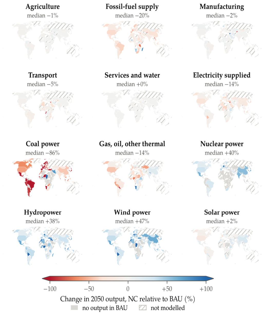
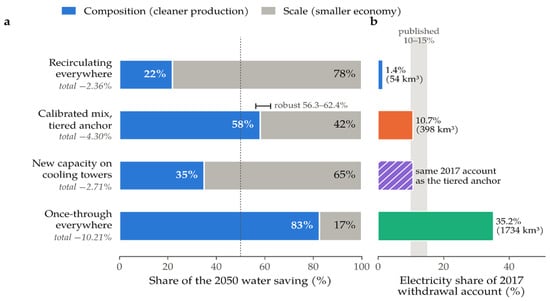
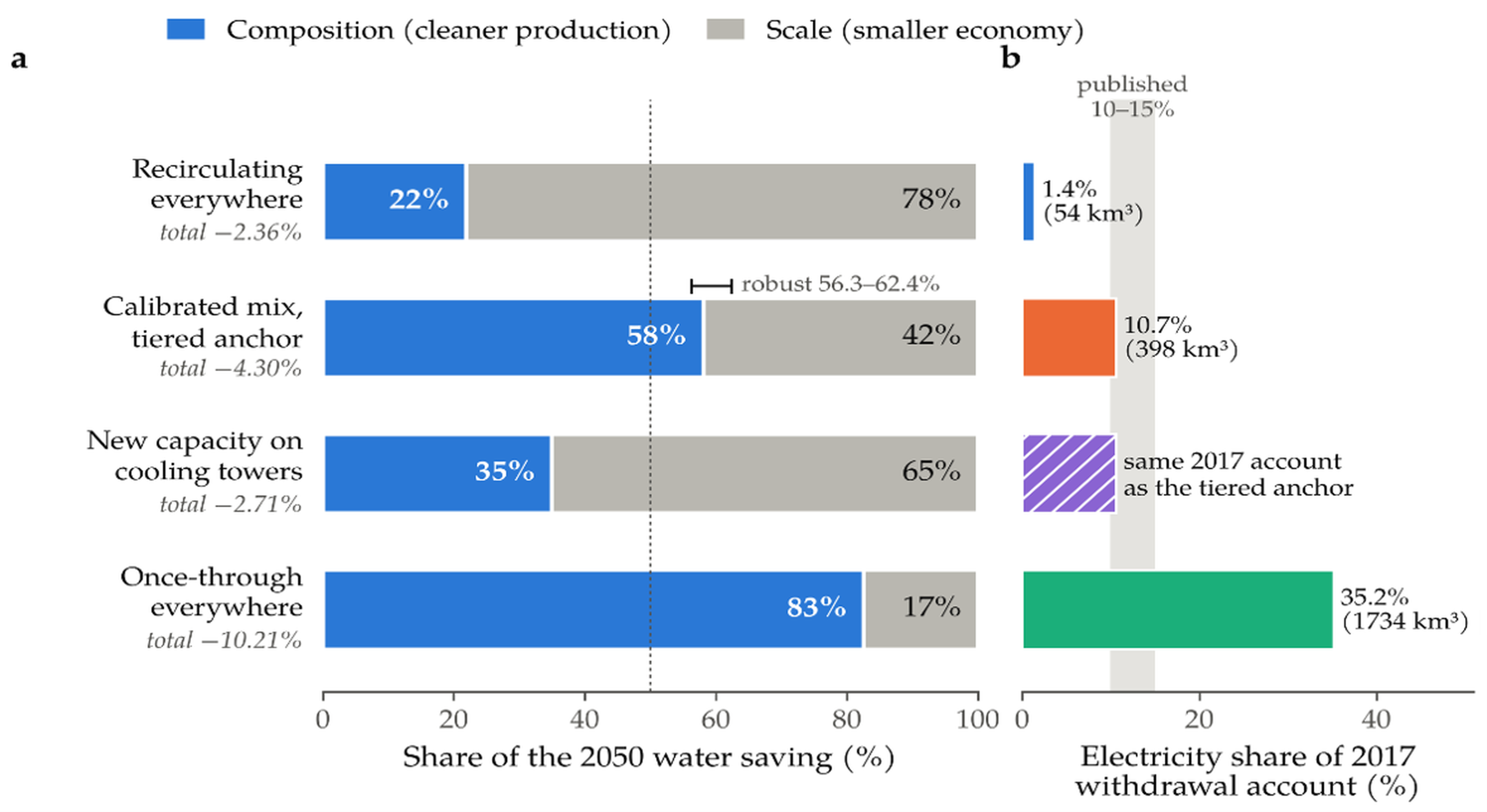
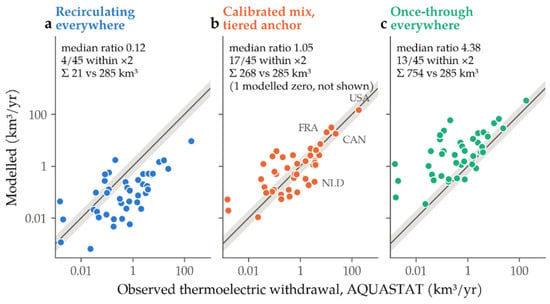
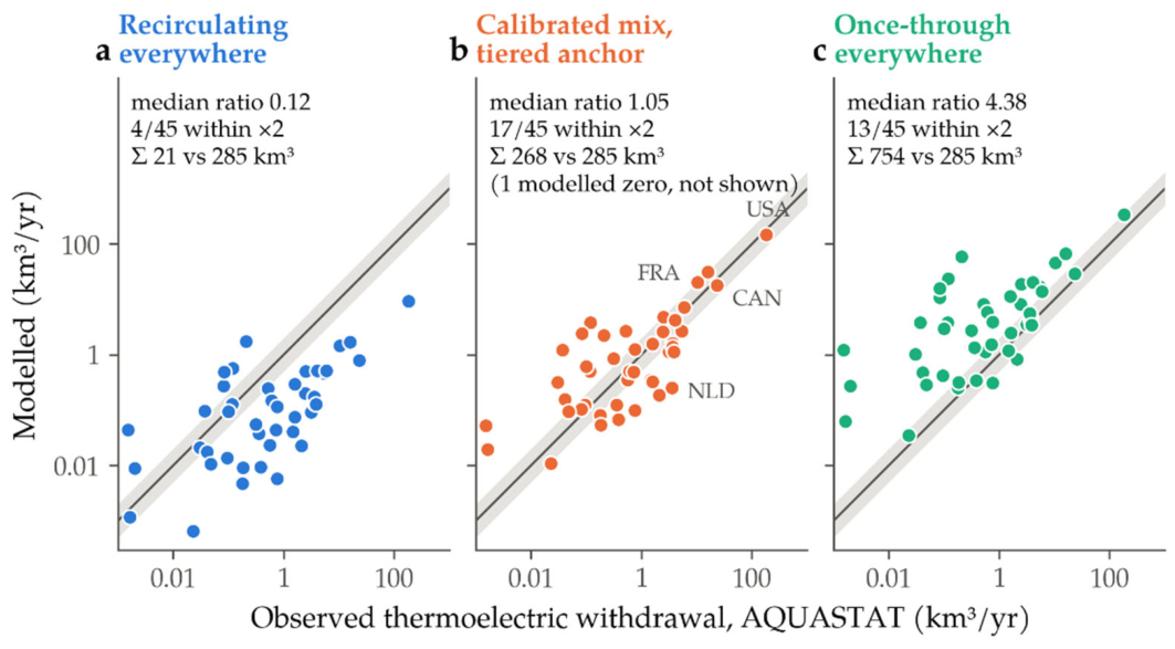
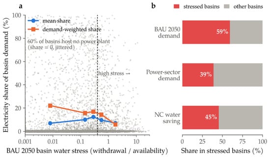
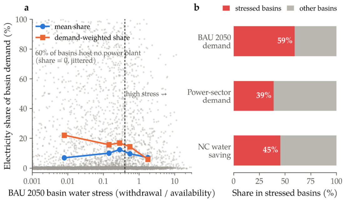

Disclaimer/Publisher’s Note: The statements, opinions and data contained in all publications are solely those of the individual author(s) and contributor(s) and not of MDPI and/or the editor(s). MDPI and/or the editor(s) disclaim responsibility for any injury to people or property resulting from any ideas, methods, instructions or products referred to in the content. |
© 2026 by the authors. Licensee MDPI, Basel, Switzerland. This article is an open access article distributed under the terms and conditions of the Creative Commons Attribution (CC BY) license.