


Abstract
Data-driven models can help represent hydrological processes at the basin scale and predict future conditions, particularly in basins where information on physical characteristics is limited. Although these models have long been used in hydrological modeling, their reliability for long-term projections under changing climatic conditions remains insufficiently understood. This study evaluates the long-term robustness and projection consistency of data-driven algorithms under climate-change conditions using two hybrid deep learning architectures: (1) a Wavelet Transform–Deep Neural Network (WT–DNN) and (2) a Convolutional Neural Network–Long Short-Term Memory–Attention Block (CNN–LSTM–AB). It also investigates whether synthetic data augmentation using a Generative Adversarial Network (GAN) during model training improves predictive performance. The study used hydrological and climatic data, including streamflow, precipitation, minimum temperature, and maximum temperature, from the Yamula Reservoir Basin, a semi-arid agricultural basin in Türkiye. The models were trained and validated for monthly streamflow using climate data from the HadGEM2–ES global circulation model for the 2000–2020 period. Long-term streamflow projections for 2021–2098 were then generated under the RCP4.5 and RCP8.5 scenarios. Model performance and robustness were assessed through sensitivity analysis, comparison of models trained with and without GAN-based data augmentation, comparison with long short-term memory (LSTM) and other recently proposed hybrid deep learning architectures, and evaluation of long-term projections against those generated by the Soil and Water Assessment Tool (SWAT) under the same future climate conditions. The results showed that WT–DNN and CNN–LSTM–AB achieved higher test-period performance than the other evaluated approaches. GAN-based data augmentation further improved model performance, reducing test root mean square error (RMSE) by 34–73% and increasing Nash–Sutcliffe efficiency (NSE) by up to 0.39. However, when applied to long-term climate projections, the relative performance of the models changed, and the superior performance of the proposed models during the historical period was not consistently maintained. The relationship between historical test performance and long-term agreement with SWAT also varied across performance metrics and climate scenarios, with no metric showing a significant relationship under both RCP4.5 and RCP8.5. These findings indicate that high test-period accuracy alone may not provide sufficient evidence of model robustness for long-term climate-change applications.
1. Introduction
Hydrologic modeling supports water resources management across a wide range of applications, including drought risk assessment, irrigation management, and water quality protection, and provides an important means of exploring the responses of hydrologic systems to climatic variability and anthropogenic impacts [1,2]. In recent decades, hydrological systems have faced increasing pressures from climate change, land-use change, and other human activities, creating a growing need for modeling approaches that can reliably represent and predict hydrological responses under changing conditions.
Process-based models have been used since the early development of hydrologic modeling. These models conceptualize hydrologic systems based on physical principles and represent the mechanisms controlling different hydrological processes [2]. Input–output relationships are described through mathematical equations based on established physical laws or theories, such as Darcy’s law and the Richards equation [3]. Reliable process-based models, such as the Soil and Water Assessment Tool (SWAT) [4,5], have been widely applied for long-term hydrological simulations and projections. However, their implementation can be challenging because they generally require extensive input data, model parameterization and calibration, and considerable expertise [3,6,7]. Model development, calibration, and validation can also be time- and resource-intensive, particularly for large or data-limited basins, which may constrain their use for applications requiring rapid assessment [4,8].
Data-driven models have emerged as an alternative approach that can address some of the limitations associated with process-based modeling. These models, including artificial intelligence approaches, learn input–output relationships directly from observations without explicitly representing the physical processes controlling the hydrologic system. Their flexibility enables them to capture complex, nonlinear, and non-stationary relationships in hydrological datasets [9], and they can achieve high predictive performance, particularly in real-time prediction and short-term forecasting applications [10,11]. However, data-driven approaches also have important limitations. Their internal structure is not directly linked to physical processes, which can limit model interpretability, process understanding, scenario analysis, and transferability to other regions or conditions [12]. Overfitting is another major concern [13], requiring strategies such as regularization, early stopping, and appropriate validation procedures to improve model generalization. More importantly, the performance of data-driven models depends strongly on the availability, length, quality, and representativeness of the data used for training. Missing observations, measurement errors, limited record lengths, and insufficient representation of rare or extreme conditions may therefore affect their predictive capability. These limitations become particularly important when models are applied beyond the range of conditions represented in the training dataset, as may occur in long-term climate-change projections. Although data-driven models have been widely applied in hydrological modeling, their reliability for such long-term projections and the potential of data augmentation to improve model performance when historical data are limited remain insufficiently understood.
In this study, the objectives are to: (1) evaluate the long-term robustness and projection consistency of data-driven algorithms under climate change; (2) propose two model architectures and compare their performance with several state-of-the-art data-driven approaches used for the same problem; (3) evaluate the effect of synthetic data augmentation to improve model training; and (4) compare the predictive performance of the proposed data-driven models with the process-based SWAT model under long-term projection conditions. Through these analyses, the study seeks to provide insight into whether strong predictive performance during historical periods translates into robust and consistent long-term projections under changing climatic conditions.
Related Work
A limited number of studies have investigated long-term streamflow forecasting using climate projections as model inputs. Lee et al. [14] applied a long short-term memory (LSTM) deep learning model, as well as the process-based SWAT model, to predict future streamflow under climate scenarios in the Mekong River Basin. They created predictions based on two representative concentration pathways (RCPs): RCP 4.5 and RCP 8.5. The results indicated that the performance of LSTM was higher than that of SWAT during the validation period, and annual future streamflow with both models did not show a statistically significant trend. The study revealed that LSTM can be used effectively for long-term hydrological forecasting when input data are limited. Wi and Steinschneider [15] evaluated whether deep learning models provide reliable streamflow predictions under climate change conditions. They also compared the results of the deep learning models with the results of three process-based models. LSTM was successful in capturing seasonal variability in streamflow; however, it produced an unrealistic streamflow pattern compared to process-based models. Khan et al. [16] used artificial neural networks (ANNs), recurrent neural networks (RNNs), and an adaptive neuro-fuzzy inference system (ANFIS) to simulate and predict streamflow in the Hunza River Basin under CMIP6 climate scenarios. The study revealed that these models can be used for analyzing the impacts of climate change when data are not sufficiently available. Recently, Nematollahi et al. [17] evaluated a hybrid deep learning model for long-term streamflow prediction under RCP4.5 and RCP8.5 climate scenarios. The results demonstrated the potential of these approaches for long-term streamflow prediction but also indicated the need for new hybrid architectures and more comprehensive comparisons of different data-driven architectures under future climate conditions.
The field of artificial intelligence is evolving, and many new architectures have recently been proposed for environmental applications. As shown in Table 1, a wide variety of deep learning and hybrid models have been applied for hydrological forecasting, including Convolutional Neural Networks (CNNs), LSTMs, Gated Recurrent Units (GRUs), Temporal Convolutional Networks (TCNs), Temporal Fusion Transformers (TFTs), encoder–decoder networks, Multilayer Perceptrons (MLPs), Support Vector Regressions (SVRs), Mamba-based models, and hybrid approaches combined with signal decomposition techniques such as Wavelet Transform (WT), Variational Mode Decomposition (VMD), and Improved Complete Ensemble Empirical Mode Decomposition with Adaptive Noise (ICEEMDAN). Most of these studies used meteorological and hydrological variables, such as precipitation, temperature, streamflow, runoff, evapotranspiration, and climate indices, as model inputs. The majority of the studies were developed for streamflow or runoff forecasting using historical datasets ranging from approximately 10 to over 40 years. These studies demonstrate the increasing use of hybrid artificial intelligence models to improve forecasting performance by combining the strengths of multiple algorithms and feature extraction techniques.
Table 1.
Summary of model architectures and methodological characteristics of related studies.
Although these approaches have shown promising results, most studies still focus on developing a single hybrid architecture without explicitly evaluating the long-term robustness of model. On the other hand, some studies suggest that high predictive performance during model development may indicate good performance under future conditions. Only a limited number of studies compared the long-term predictions with process-based models. These limitations motivated the development and evaluation of the proposed hybrid models in this study.
2. Methods
The dataset used in this study consisted of time series of streamflow and meteorological data from the Yamula Reservoir Basin in Türkiye (Figure 1). The proposed deep learning models were first trained using bias-corrected climate data for the reference period (2000–2020), with one-month-ahead streamflow as the target variable and precipitation, minimum temperature, maximum temperature, and antecedent streamflow as input variables. Following model training and evaluation, long-term streamflow projections for 2021–2098 were generated using projected meteorological variables under the selected climate-change scenarios. The following sections first describe the study area and datasets, followed by the data augmentation procedure, proposed model architectures, and methods used for model evaluation and long-term projection assessment.
Figure 1.
Location of the Yamula Reservoir Basin, showing the watershed boundary, streamflow gauging and meteorological stations, and river network. The bottom panel shows the Sentinel-2 cloudless true-color quarterly mosaic (1 October 2025).
2.1. Study Area
The Yamula Reservoir Basin is located in the upper reaches of the Kızılırmak River Basin in central Türkiye. The Kızılırmak River, the longest river located entirely within Türkiye, originates in Sivas Province and flows approximately 1355 km before discharging into the Black Sea. Along its course, the river passes through several provinces in central and northern Türkiye and drains a large area with substantial importance for regional water resources. The Kızılırmak River has been extensively developed for hydropower generation, irrigation, and water supply, with numerous dams and hydroelectric power plants constructed along its course. These multiple and competing water uses increase the importance of reliable streamflow prediction for sustainable water resources management and reservoir operation, particularly under changing climatic conditions. [35]. The present study focuses on the upstream catchment of the Yamula Reservoir, which represents the first major reservoir system along the Kızılırmak River. The study area covers approximately 15,950 km2, and the main river channel extends for about 420 km within the basin. Streamflow generated in this upstream catchment directly determines inflow to the Yamula Reservoir, making reliable long-term streamflow projections important for reservoir operation, hydropower generation, water allocation, and drought preparedness, particularly under changing climatic conditions.
The basin is characterized by a semi-arid continental climate, with cold, snowy winters and hot, dry summers. Precipitation occurs mainly during winter and spring, while streamflow is strongly influenced by seasonal snow accumulation and snowmelt. Consequently, river discharge shows considerable seasonal and interannual variability. Based on records for the 2000–2020 period, average annual precipitation was approximately 350 mm and average annual temperature was about 10.5 °C. During the same period, average streamflow was 28.5 m3/s, although substantial interannual variability was observed.
Land use within the basin is dominated by agricultural areas, rangelands, and natural vegetation, particularly at higher elevations. Agricultural activities represent an important component of water use in the basin and contribute to seasonal variations in water demand. The combined effects of climatic variability, snowmelt-driven hydrological processes, and water demand make the basin particularly relevant for evaluating the reliability of long-term streamflow projections under changing climatic conditions.
2.2. Dataset and Model Setup
Hydrological observations used in this study were obtained from the State Hydraulic Works for a streamflow gauging station located within the Yamula Reservoir Basin (D15A35-Söğütlühan) (Figure 1). This station represents different hydrological conditions across the catchment and provides long-term discharge records for model development and evaluation. The data were available on the daily timescale from 2000 to 2020. Streamflow data were converted to monthly averages before further analysis.
Data on climate were obtained from two sources. To represent the reference condition, observed precipitation, maximum temperature, and minimum temperature records were obtained from three stations (17162, 17090, 17196) (Figure 1), provided by the State Meteorology Service (MGM). The observed data were on a daily timescale and available for the 2000–2020 period. To represent projected climate, climate projection data obtained from the global circulation model HadGEM2-ES for the RCP4.5 and RCP8.5 scenarios were used. MGM produced downscaled precipitation and air temperature data until 2098 [36]. RCP4.5 represents an intermediate stabilization scenario, with greenhouse gas concentrations reaching a maximum around the middle of the century and declining gradually afterward. RCP8.5, on the other hand, represents a high-emission scenario characterized by a continued increase in greenhouse gas concentrations throughout the 21st century. For both scenarios, the output of the selected global circulation model (GCM) was dynamically downscaled over Türkiye to a spatial resolution of 20 km using the RegCM4.4 regional climate model [36]. To improve the reliability of the climate inputs, bias correction was applied using observed data from the 1980–2000 period using the quantile mapping method [37]. A multiplicative correction was applied to precipitation, whereas an additive correction was applied to minimum and maximum temperatures. The correction relationships derived for the calibration period were then applied to the RCP4.5 and RCP8.5 climate projections.
The dataset consisted of 12 variables: year, month, precipitation, maximum temperature, and minimum temperature from three meteorological stations (11 variables in total), together with monthly streamflow. The dataset was organized as a numerical time series covering two periods. The first period (2000–2020) contained observations for all 12 variables and was used for model development and evaluation. The meteorological inputs used for model development consisted of bias-corrected climate projections of precipitation, maximum temperature, and minimum temperature under the RCP4.5 and RCP8.5 scenarios. The second period (2021–2098) contained the 11 temporal and climate predictors derived from the climate projections, while observed streamflow was unavailable.
A 24-month rolling lookback window was used to construct the input sequences. Thus, for each prediction month during model development, the models used the preceding 24 months of the available variables, including antecedent streamflow, to predict streamflow for the subsequent month. For the observed period, measured streamflow values were available as antecedent inputs. For the future projection period, however, observed streamflow was unavailable. Therefore, projections were generated recursively: after initialization with the available historical observations, the streamflow predicted for each month was incorporated into the input sequence used to predict the following month. Accordingly, predicted rather than observed antecedent streamflow was progressively used throughout the 2021–2098 projection period.
For model development and evaluation, the observed dataset (2000–2020) was divided chronologically into training (70%; 2000–2014), validation (15%; 2015–2017), and testing (15%; 2018–2020) subsets. At the boundaries between these subsets, the first validation and test samples used the immediately preceding 24 months as historical inputs, including observations belonging to the preceding subset where necessary. These values represented information that would have been available before the corresponding prediction month and were used only as input history; no future observations were used to construct an earlier prediction. Thus, the chronological separation of the training, validation, and test periods was maintained.
2.3. Pre-Training and Data Augmentation
To improve the performance of the models proposed in this study, the original training dataset was augmented using a Generative Adversarial Network (GAN) [38]. The same chronological data partitioning was applied to the GAN, with 2000–2014 used for training, 2015–2017 for validation, and 2018–2020 for testing. The GAN was fitted using the 2000–2014 training partition, while the validation and test periods were used only for evaluating its performance and were not incorporated into GAN training or synthetic-data generation. The trained GAN generated an additional 20 years of synthetic monthly data, which were combined only with the original 2000–2014 training data of the proposed models. The synthetic data were not included in the validation or testing stages. Thus, the validation and test datasets consisted entirely of observed data and remained separate from the GAN-based data augmentation procedure.
The GAN architecture proposed is a conditional time-series GAN consisting of a generator and a discriminator [39] (Figure 2). The generator takes a historical input window along with a random noise vector. First, two one-dimensional (1D) convolutional layers process the input sequence to extract local patterns and short-term dependencies. The resulting feature maps are then passed through a GRU layer to capture the temporal dynamics of the sequence [40]. The GRU output combines with the noise vector to introduce randomness into the generated prediction. This combined representation is then passed through two fully connected layers to create the next-step multivariate output. In this way, the generator learns the link between a historical sequence and subsequent next step, while preserving both the temporal structure and natural variability of data.
Figure 2.
Architecture of the proposed GAN, including the generator and discriminator networks.
The discriminator part of GAN is designed to distinguish between the real and generated sequence pairs. It receives a combination of the historical input window and either the actual next observation or the generated next-step value, creating an input sequence with a length of window +1. This sequence is processed through two 1D convolutional layers (Conv1D) with Leaky Rectified Linear Unit (LeakyReLU) activations to learn distinct local features, followed by a GRU layer to capture temporal dependencies across the entire sequence. Finally, two fully connected layers produce the probability that the input sequence is real or generated. During training, the generator is optimized with an adversarial loss, which encourages it to generate realistic samples. That can fool the discriminator and a reconstruction loss, which ensures that the generated values remain close to the observed next-step values. At the same time, the discriminator is trained to correctly classify real and generated sequences.
2.4. Proposed Models
In this study, two deep learning-based models were proposed: CNN–LSTM–AB and WT–DNN.
The first proposed model, CNN–LSTM–AB, consisted of a 1D convolutional layer, a LSTM network, and multi-head attention blocks. The CNN layer first extracts local features and short-term relationships from the input sequence. The extracted features are then passed to LSTM, where LSTM captures long-term dependencies in the data. Finally, multi-head attention blocks were incorporated after the LSTM to enable the model to focus on the most relevant information from different parts of the sequence to improve the representation of temporal dependencies and the overall prediction performance [41,42] (Figure 3).
Figure 3.
The Architecture of the Proposed Hybrid CNN–LSTM–AB Model.
At first, the raw data inputs were scaled using 70% of the data for training; these data were converted into supervised examples using a fixed-length rolling window with a time step of 24 months. In the next step, 1D convolutional residual blocks were applied to learn the short-term low-level information. They capture local patterns at different temporal resolutions (Kernels 3,5,7). The output of the 1D layers was passed to stacked LSTM layers to model sequential dependencies across the window, learning long-range temporal dependencies in both directions (Forward and Backward) within each input window. A multi-head self-attention layer followed the recurrent stages to allow the network to reweight temporal contributions adaptively across the 24-step window, and the attended representation was projected through a series of fully connected layers to produce a one-step-ahead regression output. Regularization, such as dropout, batch normalization and L1/L2 kernel regularization, was applied to prevent overfitting [43].
The Adam optimizer (an adaptive learning rate algorithm that combines momentum and Root Mean Square Propagation (RMSProp) to speed up convergence) and the Huber loss (a combination of Mean Squared Error (MSE) and Mean Absolute Error (MAE) that is less sensitive to outliers than MSE and smoother than MAE) were used to improve training [44,45]. Early stopping with weight restoration and learning rate reduction at a plateau were employed to stabilize training. An early stopping mechanism was implemented in the model with a patience of 15 to prevent the models from overfitting and memorizing the training data noise. Early stopping is a regularization technique used during model training that halts the process once performance on a validation set stops improving.
The second proposed model, WT–DNN, is also based on a hybrid architecture that consists of the Wavelet Transform (WT) and Deep Neural Networks (DNNs) (Figure 4) [17]. WT is a statistical method that can examine signals at different temporal scales. WT decomposes a signal into localized components, allowing changes in both time and frequency to be evaluated simultaneously [18]. For model development, the training dataset was organized into input samples using a rolling window of 24 months.
Figure 4.
The Architecture of the Proposed WT–DNN Model adopted from [17].
In the first step, WT was applied to extract multiscale features within each time window. The approximation and detail coefficients obtained for each channel were combined and flattened into a single feature vector. The resulting features were then standardized and used as inputs to the DNN. In the second step, the DNN consisted of a 128-unit dense layer with Swish activation, L1/L2 regularization, batch normalization, and 35% dropout, followed by a 64-unit Swish dense layer with 30% dropout. A single neuron was used in the output layer for regression. This structure enables the model to capture nonlinear relationships among the multiscale features. Dropout, batch normalization, and L1/L2 regularization were used to reduce overfitting during model training [43].
As in the CNN–LSTM–AB model, the Adam optimizer and Huber loss function were used. Early stopping with weight restoration and learning-rate reduction on plateau were also applied to improve training stability and avoid overfitting.
2.5. Performance Evaluation
Model performance was evaluated using several complementary approaches (Table 2).
Table 2.
Performance evaluation methods.
First, a sensitivity analysis was conducted to investigate the effects of key training settings, including the number of epochs, batch size, and train–validation–test split ratio. The sensitivity analysis was conducted using an NVIDIA A100 GPU (40 GB HBM2e, Ampere architecture) with mixed-precision computing support [46].
Second, the contribution of GAN-based data augmentation was assessed by comparing models trained with and without synthetic data. The same model architectures, input variables, and training settings were used in both cases to ensure a consistent comparison. Changes in model performance were evaluated using the selected performance metrics for the training, validation, and test periods. This comparison was used to determine whether the inclusion of synthetic data improved model performance and reliability of predictions.
Third, the performance of the proposed models was compared with that of LSTM and other recently proposed hybrid deep learning architectures listed in Table 1. The objective was to determine whether the proposed model architectures improved accuracy and generalization compared with existing approaches. The comparison was done by using several performance metrics.
Finally, to assess the consistency of the long-term streamflow projections of the data-driven models under the RCP4.5 and RCP8.5 scenarios, their outputs were compared with those generated by a calibrated process-based SWAT model using the same climate scenarios [47]. In the study by Monga and Dadaser-Celik [47], the SWAT model was calibrated for the 2000–2013 period and validated for 2014–2020 using streamflow records from two stations. The model showed satisfactory performance during both calibration and validation, with NSE values above 0.5 and R2 values above 0.65 at both stations [48]. Further details on the SWAT model development, calibration, parameterization, and implementation are provided in Monga and Dadaser-Celik [47]. Future streamflow projections could not be evaluated against observations because observed discharge data are not available for the future period. Therefore, the comparison with SWAT does not constitute validation against observations but provides an assessment of consistency between the data-driven and process-based model projections, with SWAT serving as a process-based benchmark. Long-term streamflow projections were generated for the 2021–2098 period, and agreement with SWAT was quantified using time-series performance metrics and by examining the ability of the models to reproduce changes in streamflow patterns. To evaluate differences between the long-term monthly streamflow projections of the data-driven models and SWAT, temporal dependence in the paired-difference series was first assessed using the Ljung–Box test. As significant autocorrelation was identified, statistical significance was evaluated using a moving-block bootstrap with a 12-month block length to preserve the temporal dependence and annual structure of the monthly streamflow series. The mean paired difference and its 95% bootstrap confidence interval were calculated for each model–scenario comparison. Differences were considered statistically significant when the 95% confidence interval did not include zero. Positive differences indicate higher mean streamflow projections by the data-driven model relative to SWAT, whereas negative differences indicate lower projections.
The performance metrics, root mean squared error (RMSE) (Equation (1)), coefficient of determination (known as R-squared (R2)) (Equation (2)), Nash–Sutcliffe efficiency (NSE) (Equation (3)), percent bias (PBIAS) (Equation (4)), and Kling–Gupta Efficiency (KGE) (Equations (5)–(7)) were used during sensitivity analysis and for evaluating and comparing model performance. The RMSE is the square root of the MSE (MSE calculates the average of the squared differences between predicted and actual values) [49]. R2 is a statistical measure that shows how well the model’s predictions fit the actual data compared to a simple baseline, and NSE measures the model’s predictive performance relative to the mean of the observations. KGE evaluates model performance by jointly considering correlation, variability, and bias, while PBIAS measures the average tendency of the model to overestimate or underestimate the observed values. In the equations, yi and ȳ represent the observed and predicted values at time step i, respectively; ȳ and are the mean observed and predicted values, respectively; n is the total number of observations; R is the Pearson correlation coefficient between observed and predicted values; σŷ and σy are the standard deviations of the observed and predicted values, respectively; α is the variability ratio; and β is the bias ratio.
3. Results and Discussion
3.1. Sensitivity Analysis
In the sensitivity analysis, the effects of key training settings, including the number of epochs, batch size, and train–validation–test split ratio, were evaluated for both CNN–LSTM–AB and WT–DNN using GAN-augmented datasets. The input sequence length was fixed at 24 months, as preliminary testing of 12-, 18-, and 24-month rolling windows showed closely comparable performance, with a slight improvement for the 24-month window. The selection of the best option in the sensitivity analysis was based on the overall model performance during the training and validation periods, with particular emphasis on validation performance. RMSE, R2, NSE, PBIAS, and KGE were considered together rather than selecting an option based on a single performance metric (Table 3, Table 4 and Table 5) (Figure 5). The test dataset was not considered during the selection of model settings and was used only for the final evaluation of the selected model configuration.
Table 3.
Comparison of performance of CNN–LSTM–AB and WT–DNN models for different numbers of training epochs. The best-performing values for each model and scenario are highlighted.
Table 4.
Comparison of performance of CNN–LSTM–AB and WT–DNN models for different numbers of batches. The best-performing values for each model and scenario are highlighted.
Table 5.
Comparison of performance of CNN–LSTM–AB and WT–DNN models for different train–validation–test ratios. The best-performing values for each model and scenario are highlighted.
Figure 5.
Comparison of the validation performance of CNN–LSTM–AB and WT–DNN models under different training epochs, batch sizes, and train–validation–test splitting ratios for RCP4.5 and RCP8.5 scenarios. Model performance based on RMSE, NSE, and KGE is shown. Darker shading indicates better model performance (lower RMSE and higher NSE and KGE), while orange outlines indicate the selected hyperparameter configurations.
First, the effect of the number of epochs was evaluated by running the proposed models with 40, 80, 120, and 160 epochs (Table 3). An epoch represents one complete pass through the entire training dataset. Usually, too few epochs result in undertraining, meaning the model did not have enough passes to learn the signal in the dataset. In contrast, too many epochs may force the model to memorize the patterns and values, so the model may not train properly, which leads to overfitting [50]. During this analysis, early stopping was applied to prevent overfitting [51]. The training, validation, and testing datasets were set to 70%, 15%, and 15% of the original dataset, respectively, and the batch size was set to 16. The tested epoch values (40, 80, 120, and 160) represent maximum epoch limits; training reached the specified limit for the first two configurations, whereas the 120-epoch and 160-epoch configurations were terminated earlier (at epochs 115–120 and 150–160, respectively) by the early-stopping criterion (patience = 15). Overall, the models achieved their best performance under both RCP4.5 and RCP8.5 with a maximum epoch limit of 120, with a few exceptions (Table 3, Figure 5). The validation and testing results generally improved as the maximum epoch limit increased from 40 to 120, while further increasing the limit to 160 did not provide additional improvement and, in some cases, resulted in poorer performance.
Second, the effect of the batch sizes was evaluated by running the proposed models with 16, 32, 64, and 128 batch sizes (Table 4). The batch size refers to the number of training samples processed before the model weights are updated. Smaller batch sizes generally improve generalization but require longer training times, whereas very large batch sizes may converge to sharper minima and reduce generalization performance [52]. During the analysis, the training, validation, and testing datasets were again fixed at 70%, 15%, and 15% of the original dataset, respectively, and the epoch was fixed at 120. The results showed that batch size 16 provided the best results in the majority of cases (Table 4, Figure 5). A value of 16 can be considered a moderate batch size, which can provide a better balance between stable learning and prediction performance [53].
Third, the effects of three different train, test and validation ratios were tested (Table 5). These were 60–20–20, 70–15–15, and 80–10–10 for train–validation–test. During this analysis, the epoch was set to 120 and the batch size was fixed to 16. For both models, 70–15–15 achieved the best results. Increasing the proportion of training data generally improves the model’s performance, but it can reduce the reliability of test and validation [54]. In this study, 70–15–15 provided a good balance, where the amount of training data was maximized, while sufficient validation and testing datasets were maintained for a reliable evaluation of model performance (Table 5, Figure 5).
Overall, the best results were achieved with 120 epochs, a batch size of 16, and a 70–15–15 train–validation–test ratio. The selection was based on the performance during the training and validation periods, with particular emphasis on validation performance, considering RMSE, R2, NSE, PBIAS, and KGE together. These settings provided the best overall balance among the performance metrics under both RCP4.5 and RCP8.5. Under these conditions, during the test period, CNN–LSTM–AB provided an RMSE of 8.19 m3 s−1, an R2 of 0.79, an NSE of 0.77, a PBIAS of −8.01%, and a KGE of 0.84 under the RCP4.5 scenario. Under the RCP8.5 scenario, during test period, CNN–LSTM–AB provided an RMSE of 13.2 m3 s−1, an R2 of 0.82, an NSE of 0.83, a PBIAS of 3.5%, and a KGE of 0.89. Under the RCP4.5 scenario, during the test period, WT–DNN provided an RMSE of 12.41 m3 s−1, an R2 of 0.84, an NSE of 0.84, a PBIAS of 3.14%, and a KGE of 0.81. Under the RCP 8.5 scenario, WT–DNN’s testing performance was RMSE = 11.9 m3 s−1, R2 = 0.85, NSE = 0.85, PBIAS = 5.72%, and KGE = 0.86. It should be noted that these results represent the reference conditions, in which the RCP4.5 and RCP8.5 datasets were bias-corrected and were therefore very similar. Therefore, relatively small differences in model performance between the two scenarios were observed. Under the RCP4.5 scenario, WT–DNN showed better performance in terms R2, NSE, and PBIAS, with slightly higher R2 and NSE and lower PBIAS values than CNN–LSTM–AB. However, the performance of CNN–LSTM–AB was better in terms of RMSE and KGE. Under the RCP8.5 scenario, WT–DNN performed better in terms of RMSE, R2, and NSE, whereas CNN–LSTM–AB showed better performance based on PBIAS and KGE.
Due to the stochastic nature of deep learning model training, each model was independently trained 10 times using the same data partitions and hyperparameter configuration to evaluate the stability of model performance across different training realizations [55]. Training and test performance metrics were calculated for each run and summarized using the mean and standard deviation. For CNN–LSTM–AB, the mean training RMSE was 16.59 ± 3.36 m3/s under RCP4.5 and 14.33 ± 2.25 m3/s under RCP8.5, while the corresponding mean R2 values were 0.73 ± 0.10 and 0.82 ± 0.05, respectively. WT–DNN showed mean training RMSE values of 8.11 ± 2.87 and 8.73 ± 1.67 m3/s and mean R2 values of 0.92 ± 0.05 and 0.90 ± 0.04 under RCP4.5 and RCP8.5, respectively. For the test set, CNN–LSTM–AB showed mean RMSE values of 10.21 ± 1.10 and 14.93 ± 1.19 m3/s under RCP4.5 and RCP8.5, respectively. The corresponding mean R2 values were 0.72 ± 0.04 and 0.77 ± 0.05, while the mean NSE values were 0.73 ± 0.04 and 0.77 ± 0.04. For WT–DNN, the mean test RMSE values were 12.93 ± 0.65 and 13.61 ± 1.06 m3/s, the mean R2 values were 0.78 ± 0.03 and 0.79 ± 0.04, and the mean NSE values were 0.80 ± 0.03 and 0.80 ± 0.03 under RCP4.5 and RCP8.5, respectively. These results indicate that the general performance patterns were maintained across repeated runs, while the relatively small standard deviations of the test metrics indicate limited variability in test performance between training realizations. Previous streamflow modelling studies have similarly emphasized the consideration of performance variability when evaluating the reliability of data-driven modelling approaches [56].
Moriasi et al. [48] state that the model performance can be classified as satisfactory when R2 ≥ 0.6, NSE ≥ 0.5, and ±10 ≤ PBIAS < ±15; “good” when R2 ≥ 0.75, NSE ≥ 0.7, and ±5 ≤ PBIAS < ±10; and “very good” when R2 > 0.85, NSE > 0.80, and PBIAS < ±5. Based on personal communication with Kling, Thieming et al. [57] report that the model performance is very good when KGE ≥ 0.75 and good when KGE 0.5 ≤ KGE < 0.75. Both models demonstrated “good” performance during the testing period based on R2, NSE and PBIAS and “very good” performance under both the RCP4.5 and RCP8.5 scenarios. Since there is no universal standard for acceptable RMSE values, RMSE was also interpreted relative to the magnitude of streamflow by normalizing it by the observed streamflow range (Qmax − Qmin = 234.5 m3 s−1), resulting in the normalized RMSE (NRMSE). Lower NRMSE values, approaching zero, indicate better model performance [58]. During the testing period, NRMSE values ranged from 0.03 to 0.06, indicating that the RMSE corresponded to approximately 3–6% of the observed streamflow range.
3.2. Effect of GAN-Based Data Augmentation
The effect of GAN-based data augmentation was evaluated by training both the CNN–LSTM–AB and WT–DNN models with and without GAN-based data augmentation. Under both conditions, the number of epochs was fixed at 120, the batch size at 16, and the train–validation–test split at 70–15–15. The same optimization algorithm and training settings were used throughout all experiments to ensure a fair comparison.
The statistical characteristics of the GAN-generated data were compared with those of the observed training dataset using the mean, standard deviation, range, and coefficient of variation (Table 6). Overall, the generated temperature variables showed close agreement with the observed data under both RCP4.5 and RCP8.5. For maximum temperature, differences between the generated and observed means were less than 0.3 °C at all three stations, while the standard deviation values were also similar. Comparable agreement was observed for minimum temperature, indicating that the GAN effectively reproduced the general statistical characteristics and variability of temperature.
Table 6.
Statistical comparison of observed and GAN-generated data under RCP4.5 and RCP8.5 scenarios.
Greater differences were observed for precipitation. The generated precipitation generally had lower means and smaller ranges than the observed data, although the RCP8.5 dataset showed closer agreement in mean precipitation than RCP4.5. The generated data under both scenarios also showed lower maximum precipitation values, indicating a reduced representation of precipitation extremes.
For streamflow, the observed mean was 28.05 m3 s−1, compared with 31.45 m3 s−1 and 29.95 m3 s−1 for the GAN-generated RCP4.5 and RCP8.5 datasets, respectively. Thus, the mean streamflow was reproduced reasonably well under both scenarios, particularly RCP8.5. However, the generated streamflow showed lower variability, with SD values of 26.93 and 30.87 m3 s−1 compared with 38.15 m3 s−1 for the observed data. Similarly, maximum generated streamflows were 91.34 and 100.19 m3 s−1 under RCP4.5 and RCP8.5, respectively, compared with an observed maximum of 234.87 m3/s. Overall, the results indicate that the GAN reproduced the central tendency and general variability of the training data reasonably well, particularly for temperature and mean streamflow, but showed a lower ability to reproduce extreme precipitation and streamflow values.
GAN-based data augmentation generally improved the performance of both models, with the improvement being particularly evident for the validation and test datasets (Figure 6). For CNN–LSTM–AB under the RCP4.5 scenario, the test RMSE decreased from 29.77 m3 s−1 to 8.19 m3 s−1, while R2 increased from 0.42 to 0.79 and NSE from 0.38 to 0.77. Also test PBIAS changed from −4.27 to −8.01, while KGE decreased from 0.88 to 0.84. Under the RCP8.5 scenario, the test RMSE decreased from 15.08 m3 s−1 to 13.20 m3 s−1, accompanied by increases in R2 from 0.40 to 0.82, NSE from 0.43 to 0.83, and KGE from 0.72 to 0.89. Also test PBIAS changed from −10.3 to 3.5. A similar pattern was observed for WT–DNN. Under the RCP4.5 scenario, the test RMSE decreased from 20.42 m3 s−1 to 12.41 m3 s−1, while R2 increased from 0.44 to 0.84, NSE from 0.48 to 0.84, and KGE 0.73 to 0.81, while PBIAS changed from −10.79 to 3.14. Under the RCP8.5 scenario, all metrics provided consistent results: RMSE decreased from 18.20 m3 s−1 to 11.90 m3 s−1, with R2 increasing from 0.60 to 0.85, NSE from 0.59 to 0.85, and KGE from 0.77 to 0.86, and PBIAS changed from −11.8 to 5.72.
Figure 6.
Comparison of CNN–LSTM–AB and WT–DNN model performance with and without GAN-based data augmentation during training, validation, and testing under RCP4.5 and RCP8.5 scenarios.
Overall, these results indicate that GAN-based data augmentation generally improved model performance. RMSE, R2, and NSE improved consistently across both models and climate scenarios, whereas the effects on PBIAS and KGE were less consistent. PBIAS improved in three of the four model–scenario combinations, while KGE also improved in three cases but slightly decreased for CNN–LSTM–AB under RCP4.5. Although GAN-based augmentation improved the overall test performance, the generated data showed lower maximum streamflow values and variability than the observed data. This suggests that the improvement was mainly associated with the increased representation of more frequently occurring flow conditions and hydroclimatic relationships, which may have helped the models learn the temporal characteristics of the dataset more effectively [59]. Therefore, the improvement in overall performance metrics should not be interpreted as an improved ability to reproduce extreme high flows.
3.3. Comparison of the Performance of the Proposed Models with LSTM and with the Other Recently Proposed Hybrid Deep Learning Architectures
The performance of the CNN–LSTM–AB and WT–DNN models was compared with that of the LSTM and other recently proposed hybrid deep learning architectures listed in Table 1 (Figure 7). LSTM was selected as the baseline model because it is one of the most widely used deep learning architectures for time-series forecasting across various fields, including hydrology [60]. For others, to ensure a consistent comparison, the selected models were independently implemented using the architectural descriptions and methodological details reported in the original publications and then applied to the Yamula Reservoir Basin dataset. When multiple architectures were presented in a study, the best-performing or the most representative model was selected for implementation.
Figure 7.
Comparison of the testing performance of the proposed CNN–LSTM–AB and WT–DNN models with alternative machine learning and hybrid deep learning architectures under RCP4.5 and RCP8.5 scenarios. Model performance is presented using RMSE, R2, NSE, PBIAS, and KGE.
The results show that both proposed hybrid models generally performed well compared with the baseline LSTM model, although their relative performance varied depending on the metric and climate scenario. Under RCP4.5, the CNN–LSTM–AB model achieved the lowest RMSE (8.19 m3 s−1) and the highest KGE (0.84), while WT–DNN provided the highest R2 and NSE values (0.84 for both) and the lowest absolute PBIAS (3.14%). In comparison, LSTM produced an RMSE of 16.55 m3 s−1, R2 of 0.71, NSE of 0.70, PBIAS of −12.39%, and KGE of 0.80. Under RCP8.5, WT–DNN achieved the highest R2 and NSE values (0.85 for both), while CNN–LSTM–AB produced the lowest absolute PBIAS (3.50%) and the highest KGE (0.89). In comparison, LSTM produced R2, NSE, PBIAS, and KGE values of 0.60, 0.63, 16.12%, and 0.70, respectively. However, LSTM achieved the lowest RMSE (9.32 m3 s−1) under RCP8.5, compared with 11.90 and 13.20 m3 s−1 for WT–DNN and CNN–LSTM–AB, respectively. Overall, the proposed hybrid models showed clear improvements in R2 and NSE and generally better PBIAS and KGE values than LSTM, while their advantage in terms of RMSE was scenario-dependent. The higher performance of hybrid architectures is also consistent with findings reported in previous studies. [11,61,62,63].
The proposed models also generally performed well compared with the other architectures. Under the RCP4.5 scenario, CNN–LSTM–AB provided the lowest RMSE (8.19 m3 s−1) and, together with Stacked LSTM–Dense Multi-step, the highest KGE (0.84), while WT–DNN provided the highest R2 and NSE values (0.84 for both). Among the other methods, Encoder–MLP–Linear Regression showed good performance, with an RMSE of 12.56 m3 s−1, R2 of 0.80, and NSE of 0.83, while TFT–Prediction Head provided the lowest absolute PBIAS (2.57%). Under the RCP8.5 scenario, WT–DNN provided the highest R2 and NSE values (0.85 for both), while CNN–LSTM–AB achieved the highest KGE (0.89). CNN–LSTM–AB also produced a relatively low absolute PBIAS (3.50%). Although LSTM produced the lowest RMSE (9.32 m3 s−1), its R2 (0.60) and NSE (0.63) were considerably lower than those of the proposed models. Among the other architectures, Encoder–Decoder LSTM–Dense Regression Head performed well, with an RMSE of 12.65 m3 s−1 and R2 and NSE values of 0.80, while TFT–Prediction Head provided the lowest absolute PBIAS (1.85%) and a relatively high KGE (0.80). Overall, the proposed models showed strong and relatively balanced performance across multiple evaluation metrics under both climate scenarios, although no single model performed best according to all metrics. In general, the results support the potential of hybrid architectures to capture the complex temporal characteristics of streamflow, although their advantages depended on the performance metric and climate scenario [64]. For WT–DNN, wavelet decomposition may contribute to this performance by separating the input signal into different frequency components, allowing the DNN to learn the underlying nonlinear relationships at different temporal scales more effectively [65].
3.4. Assessment of Long-Term Projection Agreement with SWAT
To evaluate the robustness of long-term predictions, the projections of CNN–LSTM–AB, WT–DNN, and the other hybrid architectures were compared with those obtained from the SWAT model based on RMSE, NSE, R2, PBIAS and KGE and mean, maximum, minimum monthly (mean) streamflows (Figure 8). In addition, paired t-tests were performed to determine whether the projected monthly streamflows differed significantly between each data-driven model and SWAT (Table 7). It should be noted that SWAT, like any modeling approach, has its own assumptions and limitations. Therefore, this comparison did not aim to assess the accuracy of the data-driven models, but rather to evaluate their long-term projection consistency using SWAT as a process-based hydrological benchmark. It should also be noted that the literature-based hybrid architectures included in this comparison were originally developed and evaluated for predictive performance over their respective study periods, rather than for long-term climate change projections. Therefore, this comparison does not evaluate the long-term robustness claimed by the original studies. Instead, these models were included as reference data-driven approaches to examine how different model architectures perform when applied to long-term projection conditions. Several sources of uncertainty should be considered when interpreting the long-term projections.
Figure 8.
Comparison of long-term streamflow projections from the proposed CNN–LSTM–AB and WT–DNN models and alternative data-driven models with SWAT simulations under RCP4.5 and RCP8.5 scenarios based on RMSE, NSE, R2, PBIAS, and KGE.
Table 7.
Moving-block bootstrap comparison of long-term monthly streamflow projections of the data-driven models with SWAT.
Under the RCP4.5 scenario, the SWAT model projected a mean streamflow of 25.03 m3 s−1. The results showed considerable differences among the data-driven models in their agreement with the SWAT projections. The NSE values calculated between the data-driven models and SWAT ranged from −3.05 to 0.44 and R2 values from 0.07 to 0.65. The CNN–LSTM–AB model, proposed in this study, provided an NSE of 0.08 and R2 of 0.25, with a mean predicted streamflow of 33.00 m3 s−1. Its RMSE, PBIAS, and KGE relative to SWAT were 62.03 m3 s−1, 32.06%, and 0.32, respectively. WT–DNN showed comparatively better agreement with SWAT, with an NSE of 0.24 and R2 of 0.40, although its mean prediction (33.71 m3 s−1) was also higher than the SWAT mean. Its RMSE, PBIAS, and KGE were 56.31 m3 s−1, 34.76%, and 0.37, respectively. Among the benchmark models, AB–LSTM provided the highest NSE (0.44), while LSTM–Improved Complete Ensemble Empirical Mode Decomposition with Adaptive Noise–Sample Entropy–Gini showed the highest R2 (0.65). The latter also produced a mean streamflow of 26.25 m3 s−1, which was close to the SWAT mean. AB–LSTM also showed the lowest absolute PBIAS (0.82%), while TCN provided the highest KGE (0.51).
Under the RCP8.5 scenario, the SWAT model projected a mean streamflow of 25.71 m3 s−1. The agreement of CNN–LSTM–AB with SWAT was considerably higher compared with RCP4.5. The NSE value was 0.36 and R2 was 0.38. Its mean predicted streamflow was 26.26 m3 s−1, closely corresponding to the SWAT mean. The model also provided an RMSE of 52.95 m3 s−1, a PBIAS of 2.23%, and a KGE of 0.49. In contrast, WT–DNN produced an NSE of 0.24 and R2 of 0.34, with a higher mean streamflow of 32.50 m3 s−1. Its RMSE, PBIAS, and KGE were 57.81 m3 s−1, 26.46%, and 0.49, respectively. Among the benchmark models, Encoder–MLP–Linear Regression [20] provided the highest NSE and R2, with values of 0.45 for both, and produced a mean streamflow of 26.25 m3 s−1, which was also very close to the SWAT projection. It also produced a low PBIAS of 2.16% and a KGE of 0.45. LSTM–Improved Complete Ensemble Empirical Mode Decomposition with Adaptive Noise–Sample Entropy–Gini also showed relatively strong agreement, with an NSE of 0.41 and R2 of 0.42. Overall, CNN–LSTM–AB showed relatively balanced agreement with SWAT under RCP8.5, with a mean streamflow close to the SWAT mean, low PBIAS, and the highest KGE (0.49, together with WT–DNN) among the evaluated models.
The minimum and maximum projected flows further provide insight into these differences. SWAT simulated a wider streamflow range, from 0 to 291.90 m3 s−1 under the RCP4.5 scenario and from 0 to 299.50 m3 s−1 under the RCP8.5 scenario. In contrast, the data-driven models generally produced streamflow values in a narrower range. In particular, peak streamflow values were lower. None of the evaluated data-driven architectures reproduced maximum flows approaching those simulated by SWAT under either scenario, while several models also produced minimum flows above zero. The highest maximum flow among the data-driven models was 163.26 m3 s−1 under RCP4.5 (Wavelet Transform–ANN) and 156.29 m3 s−1 under RCP8.5 (TFT–Prediction Head), both substantially below the corresponding SWAT maxima. Thus, even models that showed relatively good agreement with SWAT in terms of NSE, R2, PBIAS, KGE, or mean streamflow did not necessarily reproduce the full range of hydrological variability represented by the process-based model. In particular, the substantially lower maxima suggest that the data-driven models tend to attenuate high-flow conditions when extended to long-term projections.
To evaluate differences between the long-term monthly streamflow projections of the data-driven models and SWAT, a moving-block bootstrap method was used. A block length of 12 months was used to preserve the temporal dependence and annual structure of the monthly streamflow series. The mean paired difference and its 95% bootstrap confidence interval were calculated for each model–scenario comparison. A difference was considered statistically significant when the 95% confidence interval did not include zero. Positive differences indicate higher mean streamflow projections by the data-driven model relative to SWAT, whereas negative differences indicate lower projections. (Table 7). The moving-block bootstrap analysis showed significant differences in mean monthly streamflow between SWAT and most of the data-driven model projections. Under RCP4.5, significant differences were identified for 14 of the 19 models, while under RCP8.5, significant differences were observed for 15 models. For the proposed models, CNN–LSTM–AB produced a significantly higher mean streamflow than SWAT under RCP4.5 (mean difference = 8.02 m3/s; 95% CI: 5.33–10.34 m3/s), whereas no significant average difference was detected under RCP8.5 (0.57 m3/s; 95% CI: −1.76–2.50 m3/s). WT–DNN produced significantly higher mean streamflows than SWAT under both RCP4.5 (8.69 m3/s; 95% CI: 6.44–10.64 m3/s) and RCP8.5 (6.80 m3/s; 95% CI: 4.43–8.78 m3/s).
The differences in extreme high-flow projections, together with the significant differences in mean monthly streamflow identified for most model–scenario comparisons using the moving-block bootstrap, indicate that the long-term projections of the data-driven models can diverge from those of SWAT. Several factors may explain these differences. Deep learning models learn statistical relationships from the range and frequency of conditions represented in the training data. Extreme high-flow events are relatively infrequent and therefore contribute less to model optimization than the more frequently occurring low and moderate flows [66]. Consequently, predictions tend to remain closer to the range most strongly represented during training, limiting the ability of the models to reproduce unusually high flows under future climatic conditions [67]. The use of the Huber loss function may also contribute to this behavior. Huber loss behaves quadratically for small residuals but applies a linear penalty to large residuals, thereby reducing the influence of extreme errors during model optimization [68].
These limitations may become particularly important for long-term climate projections because future combinations of precipitation and temperature may extend beyond, or differ from, those represented during model training. Under such conditions, the models are required to extrapolate learned relationships rather than interpolate within familiar conditions, increasing uncertainty in the prediction of extremes. The higher maximum flows simulated by SWAT should not necessarily be considered the true future values; however, the large differences between the process-based and data-driven projections indicate that the latter should be used cautiously for applications in which high-flow extremes are of primary importance.
An additional source of uncertainty arises from the way antecedent streamflow is incorporated into the long-term projections. For the historical period, observed antecedent streamflow was available as part of the input sequence, whereas future projections necessarily relied on previously predicted streamflow because observations were unavailable. Accordingly, the long-term projections were generated recursively, with each predicted streamflow value contributing to the input sequence for the subsequent prediction. This approach enables the trained models to be applied continuously over the future projection period. However, the use of predicted rather than observed antecedent streamflow introduces additional uncertainty compared with the historical model evaluation, as prediction errors may propagate through successive time steps. Therefore, the performance metrics obtained for the testing period primarily characterize the models under observed historical input conditions, while the long-term projections should be interpreted considering the additional uncertainty associated with recursive forecasting.
The variability observed across repeated training runs indicates that stochastic model training contributes to uncertainty in model performance. In addition, uncertainty may arise from the GAN-generated training samples, bias correction of the climate inputs, and the use of a single GCM–RCM chain.
To examine whether historical model performance was associated with long-term projection performance, Pearson correlation coefficients were calculated between the corresponding historical and long-term performance metrics (RMSE, NSE, R2, PBIAS, and KGE) across the evaluated models. The analysis was performed separately for RCP4.5 and RCP8.5. Under RCP4.5, significant positive correlations were observed for NSE (r = 0.713, p < 0.001) and R2 (r = 0.460, p = 0.047), while the correlations for RMSE (r = 0.438, p = 0.061), PBIAS (r = 0.034, p = 0.891), and KGE (r = 0.248, p = 0.306) were not statistically significant. Under RCP8.5, significant correlations were observed for PBIAS (r = −0.468, p = 0.043) and KGE (r = 0.529, p = 0.020), whereas the correlations for RMSE (r = 0.143, p = 0.559), NSE (r = 0.323, p = 0.178), and R2 (r = 0.361, p = 0.129) were not statistically significant. Overall, none of the performance metrics showed a statistically significant relationship between historical and long-term performance under both climate scenarios. These results indicate that the relationship between historical test performance and long-term agreement with SWAT was metric- and scenario-dependent, supporting the conclusion that historical performance alone may not provide a consistent indication of long-term projection performance.
Overall, these results suggest that good overall validation performance alone may not be sufficient to establish the robustness of data-driven models for long-term hydrological projections, particularly for conditions that are poorly represented in the historical training record. A model demonstrating relatively higher performance does not necessarily provide the closest mean streamflow or reproduce the range of flows represented by SWAT. Similarly, a model producing a mean streamflow close to SWAT may still differ considerably in its temporal dynamics and high-flow behavior. Therefore, evaluating long-term robustness solely on the basis of conventional performance statistics may provide an incomplete picture of model behavior under future climatic conditions. The combined consideration of temporal agreement, bias, overall agreement, long-term mean conditions, and the range of projected flows provides a more comprehensive assessment of the behavior of data-driven models when extrapolated beyond the conditions represented in their historical training data.
4. Conclusions
This study evaluated and compared the long-term robustness and projection consistency of data-driven algorithms under climate-change conditions by employing two hybrid architectures, CNN–LSTM–AB and WT–DNN, to simulate monthly streamflow. Data augmentation was also applied using a GAN framework to improve model training and generalization. These models were evaluated for parameter sensitivity, predictive accuracy, and consistency with a process-based model. In addition, their long-term performance was compared with that of other data-driven approaches available in the literature.
Key findings can be listed as follows:
- •
- Both the CNN–LSTM–AB and WT–DNN architectures provided high model accuracy during training, validation, and testing and generally performed well compared with the selected hybrid architectures reported in the literature. These results demonstrate the potential of CNN–LSTM–AB and WT–DNN for streamflow prediction under historical conditions.
- •
- Synthetic data augmentation using the GAN framework generally improved model performance and showed potential when training data are limited. However, the effectiveness of GAN-based augmentation depends on the quality and representativeness of the available observations. When observed data are sparse, noisy, or of poor quality, GAN-generated samples may reproduce or amplify existing errors and introduce unrealistic temporal patterns. Future studies should therefore further evaluate the quality and temporal characteristics of GAN-generated data and investigate the conditions under which GAN-based augmentation provides reliable improvements in hydrological applications.
- •
- Historical predictive accuracy was not a consistent indicator of long-term projection performance. Comparison with SWAT showed that the relationship between historical test performance and long-term agreement with SWAT varied depending on the performance metric and climate scenario, with none of the evaluated metrics showing a significant relationship under both RCP4.5 and RCP8.5. Therefore, high predictive accuracy during historical testing does not necessarily indicate consistent model behavior over long-term future projections. Agreement with SWAT should not itself be interpreted as evidence of greater future reliability, but rather as a process-based benchmark for evaluating the consistency of long-term projection behavior among the models.
Future studies should focus on improving the long-term robustness of data-driven models, including the incorporation of physical constraints to better represent hydrological processes under conditions outside the historical range. In addition, quantitative assessment of covariate shift between historical training data and future climate inputs could provide further insight into model behavior under out-of-distribution conditions. Long-term model behavior should also be evaluated using multiple indicators, including temporal agreement, mean streamflow, variability, and extreme flows. Finally, as this study was based on a single GCM–RCM chain (HadGEM2-ES/RegCM4.4), future studies should consider multiple climate models or multi-model ensembles to assess model behavior under a wider range of future climate conditions.
Author Contributions
Conceptualization, A.R.N., M.C., and F.D.-C.; methodology, A.R.N., M.C., and F.D.-C.; formal analysis, A.R.N.; writing—original draft preparation, A.R.N. writing—review and editing, M.C., and F.D.-C.; funding acquisition, F.D.-C. All authors have read and agreed to the published version of the manuscript.
Funding
This study was supported by Erciyes University Research Fund (FBA-2026-15752).
Data Availability Statement
The data that support the findings of this study are available on request from the corresponding author.
Conflicts of Interest
The authors do not declare any competing interests.
References
- O’Connell, P.E.; Todini, E. Modelling of rainfall, flow and mass transport in hydrological systems: An overview. J. Hydrol. 1996, 175, 3–16. [Google Scholar] [CrossRef] [Scilit]
- Singh, V.P.; Woolhiser, D.A. Mathematical Modeling of Watershed Hydrology. J. Hydrol. Eng. 2002, 7, 270–292. [Google Scholar] [CrossRef] [Scilit]
- Clark, M.P.; Bierkens, M.F.P.; Samaniego, L.; Woods, R.A.; Uijlenhoet, R.; Bennett, K.E.; Pauwels, V.R.N.; Cai, X.; Wood, A.W.; Peters-Lidard, C.D. The evolution of process-based hydrologic models: Historical challenges and the collective quest for physical realism. Hydrol. Earth Syst. Sci. 2017, 21, 3427–3440. [Google Scholar] [CrossRef] [Scilit] [PubMed]
- Özdoğan-Sarıkoç, G.; Dadaser-Celik, F. Physically based vs. data-driven models for streamflow and reservoir volume prediction at a data-scarce semi-arid basin. Environ. Sci. Pollut. Res. 2024, 31, 39098–39119. [Google Scholar] [CrossRef] [Scilit] [PubMed]
- Aibaidula, D.; Ates, N.; Dadaser-Celik, F. Modelling climate change impacts at a drinking water reservoir in Turkey and implications for reservoir management in semi-arid regions. Environ. Sci. Pollut. Res. 2023, 30, 13582–13604. [Google Scholar] [CrossRef] [Scilit] [PubMed]
- Herrera, P.A.; Marazuela, M.A.; Hofmann, T. Parameter estimation and uncertainty analysis in hydrological modeling. WIREs Water 2022, 9, e1569. [Google Scholar] [CrossRef] [Scilit]
- Refsgaard, J.C. Parameterisation, calibration and validation of distributed hydrological models. J. Hydrol. 1997, 198, 69–97. [Google Scholar] [CrossRef] [Scilit]
- Aibaidula, D.; Ates, N.; Dadaser-Celik, F. Uncertainty analysis for streamflow modeling using multiple optimization algorithms at a data-scarce semi-arid region: Altınapa Reservoir Watershed, Turkey. Stoch. Environ. Res. Risk Assess. 2023, 37, 1997–2011. [Google Scholar] [CrossRef] [Scilit]
- Yaseen, Z.M.; El-shafie, A.; Jaafar, O.; Afan, H.A.; Sayl, K.N. Artificial intelligence based models for stream-flow forecasting: 2000–2015. J. Hydrol. 2015, 530, 829–844. [Google Scholar] [CrossRef] [Scilit]
- Fahimi, F.; Yaseen, Z.M.; El-shafie, A. Application of soft computing based hybrid models in hydrological variables modeling: A comprehensive review. Theor. Appl. Climatol. 2017, 128, 875–903. [Google Scholar] [CrossRef] [Scilit]
- Sarıkoç, M.; Celik, M. PCA-ICA-LSTM: A Hybrid Deep Learning Model Based on Dimension Reduction Methods to Predict S&P 500 Index Price. Comput. Econ. 2025, 65, 2249–2315. [Google Scholar] [CrossRef] [Scilit]
- Elshorbagy, A.; Corzo, G.; Srinivasulu, S.; Solomatine, D.P. Experimental investigation of the predictive capabilities of data driven modeling techniques in hydrology—Part 2: Application. Hydrol. Earth Syst. Sci. 2010, 14, 1943–1961. [Google Scholar] [CrossRef] [Scilit]
- Abrahart, R.J.; Anctil, F.; Coulibaly, P.; Dawson, C.W.; Mount, N.J.; See, L.M.; Shamseldin, A.Y.; Solomatine, D.P.; Toth, E.; Wilby, R.L. Two decades of anarchy? Emerging themes and outstanding challenges for neural network river forecasting. Prog. Phys. Geogr. Earth Environ. 2012, 36, 480–513. [Google Scholar] [CrossRef] [Scilit]
- Lee, D.; Lee, G.; Kim, S.; Jung, S. Future Runoff Analysis in the Mekong River Basin under a Climate Change Scenario Using Deep Learning. Water 2020, 12, 1556. [Google Scholar] [CrossRef] [Scilit]
- Wi, S.; Steinschneider, S. Assessing the Physical Realism of Deep Learning Hydrologic Model Projections Under Climate Change. Water Resour. Res. 2022, 58, e2022WR032123. [Google Scholar] [CrossRef] [Scilit]
- Khan, M.; Khan, A.U.; Khan, S.; Khan, F.A. Assessing the impacts of climate change on streamflow dynamics: A machine learning perspective. Water Sci. Technol. 2023, 88, 2309–2331. [Google Scholar] [CrossRef] [Scilit] [PubMed]
- Nematollahi, A.R.; Celik, M.; Dadaser-Celik, F. Deep Learning Approach for Monthly Streamflow Prediction in Yamula Reservoir Watershed in Türkiye. Environ. Earth Sci. Proc. 2026, 44, 19. [Google Scholar] [CrossRef] [Scilit]
- Graf, R.; Zhu, S.; Sivakumar, B. Forecasting river water temperature time series using a wavelet–neural network hybrid modelling approach. J. Hydrol. 2019, 578, 124115. [Google Scholar] [CrossRef] [Scilit]
- Shahariar, S.; Zobeyer, H.; Jahan, N. Deep learning-based prediction of flood hazard and future streamflow changes in the Brahmaputra River Basin under CMIP6 climate change scenarios. J. Hydrol. Reg. Stud. 2026, 65, 103357. [Google Scholar] [CrossRef] [Scilit]
- Fang, Z.; Qu, S.; Yang, X.; Li, Z.; Shi, P.; Xu, X.; Yu, Y. Using tide for rainfall runoff simulation with feature projection and reversible instance normalization. Sci. Rep. 2025, 15, 7200. [Google Scholar] [CrossRef] [Scilit] [PubMed]
- Han, D.; Liu, P.; Xie, K.; Li, H.; Xia, Q.; Cheng, Q.; Wang, Y.; Yang, Z.; Zhang, Y.; Xia, J. An attention-based LSTM model for long-term runoff forecasting and factor recognition. Environ. Res. Lett. 2023, 18, 024004. [Google Scholar] [CrossRef] [Scilit]
- Ali, A.J.; Ahmed, A.A.; Abbod, M.F. Groundwater level predictions in the Thames Basin, London over extended horizons using Transformers and advanced machine learning models. J. Clean. Prod. 2024, 484, 144300. [Google Scholar] [CrossRef] [Scilit]
- Zhang, Y.; Ragettli, S.; Molnar, P.; Fink, O.; Peleg, N. Generalization of an Encoder-Decoder LSTM model for flood prediction in ungauged catchments. J. Hydrol. 2022, 614, 128577. [Google Scholar] [CrossRef] [Scilit]
- Jesus, G.; Mardani, Z.; Alves, E.; Oliveira, A. Deep Learning-Based River Flow Forecasting with MLPs: Comparative Exploratory Analysis Applied to the Tejo and the Mondego Rivers. Sensors 2025, 25, 2154. [Google Scholar] [CrossRef] [Scilit] [PubMed]
- Xu, Y.; Hu, C.; Wu, Q.; Li, Z.; Jian, S.; Chen, Y. Application of temporal convolutional network for flood forecasting. Hydrol. Res. 2021, 52, 1455–1468. [Google Scholar] [CrossRef] [Scilit]
- Li, J.; Ai, P.; Xiong, C.; Song, Y. Leveraging multi-source data and teleconnection indices for enhanced runoff prediction using coupled deep learning models. Sci. Rep. 2025, 15, 14732. [Google Scholar] [CrossRef] [Scilit] [PubMed]
- Mirzaei, M.; Yu, H.; Dehghani, A.; Galavi, H.; Shokri, V.; Mohsenzadeh Karimi, S.; Sookhak, M. A Novel Stacked Long Short-Term Memory Approach of Deep Learning for Streamflow Simulation. Sustainability 2021, 13, 13384. [Google Scholar] [CrossRef] [Scilit]
- Jia, D.; Li, W.; Huang, D.; Chen, S. Daily runoff prediction based on lightweight Mamba with partial normalization. Hydrol. Res. 2024, 55, 1182–1196. [Google Scholar] [CrossRef] [Scilit]
- Xu, D.-M.; Li, Z.; Wang, W.-C. An ensemble model for monthly runoff prediction using least squares support vector machine based on variational modal decomposition with dung beetle optimization algorithm and error correction strategy. J. Hydrol. 2024, 629, 130558. [Google Scholar] [CrossRef] [Scilit]
- Rasiya Koya, S.; Roy, T. Temporal Fusion Transformers for streamflow Prediction: Value of combining attention with recurrence. J. Hydrol. 2024, 637, 131301. [Google Scholar] [CrossRef] [Scilit]
- Huang, C.; Zhou, T.; Li, W.; Yu, H.; Li, R.; Fang, J. A coupled model integrating dual attention mechanism into BiGRU-RED for multi-step-ahead streamflow forecasting. J. Hydrol. 2024, 645, 132137. [Google Scholar] [CrossRef] [Scilit]
- Xu, D.-M.; Hong, Y.-H.; Wang, W.-C.; Li, Z.; Wang, J. A novel daily runoff forecasting model based on global features and enhanced local feature interpretation. J. Hydrol. 2024, 645, 132227. [Google Scholar] [CrossRef] [Scilit]
- Akbarian, M.; Saghafian, B.; Golian, S. Monthly streamflow forecasting by machine learning methods using dynamic weather prediction model outputs over Iran. J. Hydrol. 2023, 620, 129480. [Google Scholar] [CrossRef] [Scilit]
- Apaydin, H.; Sibtain, M. A multivariate streamflow forecasting model by integrating improved complete ensemble empirical mode decomposition with additive noise, sample entropy, Gini index and sequence-to-sequence approaches. J. Hydrol. 2021, 603, 126831. [Google Scholar] [CrossRef] [Scilit]
- Varol, M.; Kaçar, E.; Sünbül, M.R.; Md Towfiqul Islam, A.R. Levels of metals and elements in tissues of fish species in the Kızılırmak River (Turkey) and assessment of health risks and nutritional benefits. Environ. Res. 2022, 214, 113791. [Google Scholar] [CrossRef] [Scilit] [PubMed]
- Akcakaya, A.; Sümer, U.M.; Demircan, M.; Demir, O.; Atay, H.; Eskioglu, O.; Gurkan, H.; Yazıcı, B.; Kocaturk, A.; Sensoy, S.; et al. Yeni Senaryolar ile Türkiye Iklim Projeksiyonlari ve Iklim Değişikliği; State Meteorology Service: Ankara, Türkiye, 2015. [Google Scholar]
- Gudmundsson, L.; Bremnes, J.B.; Haugen, J.E.; Engen-Skaugen, T. Technical Note: Downscaling RCM precipitation to the station scale using statistical transformations—A comparison of methods. Hydrol. Earth Syst. Sci. 2012, 16, 3383–3390. [Google Scholar] [CrossRef] [Scilit]
- Moeini, F.; Ershadnia, R.; Rubinstein, R.L.; Versteeg, R.; Li, P.; McGarr, J.T.; Meyal, A.; Wallace, C.D.; Dai, Z.; Carroll, K.C.; et al. Employing generative adversarial neural networks as surrogate model for reactive transport modeling in the hyporheic zone. J. Hydrol. 2024, 639, 131485. [Google Scholar] [CrossRef] [Scilit]
- Iglesias, G.; Talavera, E.; Díaz-Álvarez, A. A survey on GANs for computer vision: Recent research, analysis and taxonomy. Comput. Sci. Rev. 2023, 48, 100553. [Google Scholar] [CrossRef] [Scilit]
- Al-Smadi, M.; Hammad, M.M.; Al-Zboon, S.a.A.; Al-Tawalbeh, S.; Cambria, E. Gated recurrent unit with multilingual universal sentence encoder for Arabic aspect-based sentiment analysis. Knowl. -Based Syst. 2023, 261, 107540. [Google Scholar] [CrossRef] [Scilit]
- Ni, L.; Wang, D.; Singh, V.P.; Wu, J.; Wang, Y.; Tao, Y.; Zhang, J. Streamflow and rainfall forecasting by two long short-term memory-based models. J. Hydrol. 2020, 583, 124296. [Google Scholar] [CrossRef] [Scilit]
- Niu, Z.; Zhong, G.; Yu, H. A review on the attention mechanism of deep learning. Neurocomputing 2021, 452, 48–62. [Google Scholar] [CrossRef] [Scilit]
- Yang, M.; Lim, M.K.; Qu, Y.; Li, X.; Ni, D. Deep neural networks with L1 and L2 regularization for high dimensional corporate credit risk prediction. Expert Syst. Appl. 2023, 213, 118873. [Google Scholar] [CrossRef] [Scilit]
- Feng, D.; Liu, J.; Lawson, K.; Shen, C. Differentiable, Learnable, Regionalized Process-Based Models With Multiphysical Outputs can Approach State-Of-The-Art Hydrologic Prediction Accuracy. Water Resour. Res. 2022, 58, e2022WR032404. [Google Scholar] [CrossRef] [Scilit]
- Kim, D.; Lee, J.; Kim, J.; Lee, M.; Wang, W.; Kim, H.S. Comparative analysis of long short-term memory and storage function model for flood water level forecasting of Bokha stream in NamHan River, Korea. J. Hydrol. 2022, 606, 127415. [Google Scholar] [CrossRef] [Scilit]
- Choquette, J.; Gandhi, W.; Giroux, O.; Stam, N.; Krashinsky, R. NVIDIA A100 Tensor Core GPU: Performance and Innovation. IEEE Micro 2021, 41, 29–35. [Google Scholar] [CrossRef] [Scilit]
- Monga, E.; Dadaser-Celik, F. Modeling of Hydrological Processes and Sediment Transport in the Yamula Reservoir Basin; Erciyes University: Kayseri, Türkiye, 2026. [Google Scholar]
- Moriasi, D.N.; Gitau, M.W.; Pai, N.; Daggupati, P. Hydrologic and Water Quality Models: Performance Measures and Evaluation Criteria. Trans. ASABE 2015, 58, 1763–1785. [Google Scholar] [CrossRef] [Scilit]
- Tran, V.N.; Kim, J. A robust surrogate data assimilation approach to real-time forecasting using polynomial chaos expansion. J. Hydrol. 2021, 598, 126367. [Google Scholar] [CrossRef] [Scilit]
- Goodfellow, I.; Bengio, Y.; Courville, A.; Bengio, Y. Deep Learning; MIT Press: Cambridge, UK, 2016; Volume 1. [Google Scholar]
- Prince, S.J. Understanding Deep Learning; MIT Press: Cambridge, UK, 2023. [Google Scholar]
- Bishop, C.M.; Bishop, H. Deep Learning: Foundations and Concepts; Springer: Cham, Switzerland, 2024; Volume 1. [Google Scholar]
- He, F.; Tao, D. Foundations of Deep Learning; Springer: Berlin/Heidelberg, Germany, 2025. [Google Scholar]
- Collins, G.S.; Dhiman, P.; Ma, J.; Schlussel, M.M.; Archer, L.; Van Calster, B.; Harrell, F.E., Jr.; Martin, G.P.; Moons, K.G.M.; van Smeden, M.; et al. Evaluation of clinical prediction models (part 1): From development to external validation. BMJ 2024, 384, e074819. [Google Scholar] [CrossRef] [Scilit] [PubMed]
- Yilmaz, M.U.; Alakus, T.B. Neural circuit policy and hybrid deep learning models for enhanced meteorological drought forecasting performance. Appl. Soft Comput. 2026, 193, 114844. [Google Scholar] [CrossRef] [Scilit]
- Yilmaz, M.U.; Aksu, H.; Onoz, B.; Selek, B. An Effective Framework for Improving Performance of Daily Streamflow Estimation Using Statistical Methods Coupled with Artificial Neural Network. Pure Appl. Geophys. 2023, 180, 3639–3654. [Google Scholar] [CrossRef] [Scilit]
- Thiemig, V.; Rojas, R.; Zambrano-Bigiarini, M.; De Roo, A. Hydrological evaluation of satellite-based rainfall estimates over the Volta and Baro-Akobo Basin. J. Hydrol. 2013, 499, 324–338. [Google Scholar] [CrossRef] [Scilit]
- Dang, Q.T.; Laux, P.; Kunstmann, H. Future high- and low-flow estimations for Central Vietnam: A hydro-meteorological modelling chain approach. Hydrol. Sci. J. 2017, 62, 1867–1889. [Google Scholar] [CrossRef] [Scilit]
- Bandara, K.; Hewamalage, H.; Liu, Y.-H.; Kang, Y.; Bergmeir, C. Improving the accuracy of global forecasting models using time series data augmentation. Pattern Recognit. 2021, 120, 108148. [Google Scholar] [CrossRef] [Scilit]
- Tripathy, K.P.; Mishra, A.K. Deep learning in hydrology and water resources disciplines: Concepts, methods, applications, and research directions. J. Hydrol. 2024, 628, 130458. [Google Scholar] [CrossRef] [Scilit]
- Ozkok, F.O.; Celik, M. A hybrid CNN-LSTM model for high resolution melting curve classification. Biomed. Signal Process. Control 2022, 71, 103168. [Google Scholar] [CrossRef] [Scilit]
- Altarawneh, E.S.; Sharil, S.; Razali, S.F.M.; Ahmed, A.N.; El-Shafie, A. Hybrid hydrological modeling: Integration of machine learning and conventional hydrology. Phys. Chem. Earth Parts A/B/C 2025, 141, 104150. [Google Scholar] [CrossRef] [Scilit]
- Chen, H.; Huang, J.J.; Dash, S.S.; Wei, Y.; Li, H. A hybrid deep learning framework with physical process description for simulation of evapotranspiration. J. Hydrol. 2022, 606, 127422. [Google Scholar] [CrossRef] [Scilit]
- Asadnia, M.; Razmjou, A.; Beheshti, A. Artificial Intelligence and Data Science in Environmental Sensing; Academic Press: Cambridge, MA, USA, 2022. [Google Scholar]
- Mehra, M.; Mehra, V.; Ahmad, M. Wavelets Theory and Its Applications; Springer: Berlin/Heidelberg, Germany, 2018. [Google Scholar]
- Baste, S.; Klotz, D.; Acuña Espinoza, E.; Bardossy, A.; Loritz, R. Unveiling the limits of deep learning models in hydrological extrapolation tasks. Hydrol. Earth Syst. Sci. 2025, 29, 5871–5891. [Google Scholar] [CrossRef] [Scilit]
- Xie, K.; Liu, P.; Zhang, J.; Han, D.; Wang, G.; Shen, C. Physics-guided deep learning for rainfall-runoff modeling by considering extreme events and monotonic relationships. J. Hydrol. 2021, 603, 127043. [Google Scholar] [CrossRef] [Scilit]
- Dahal, K.; Gupta, A.; Bokati, L.; Kumar, S. Ensemble streamflow forecasting with diverse loss functions. Appl. Soft Comput. 2026, 198, 115276. [Google Scholar] [CrossRef] [Scilit]
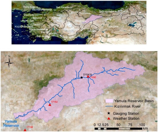
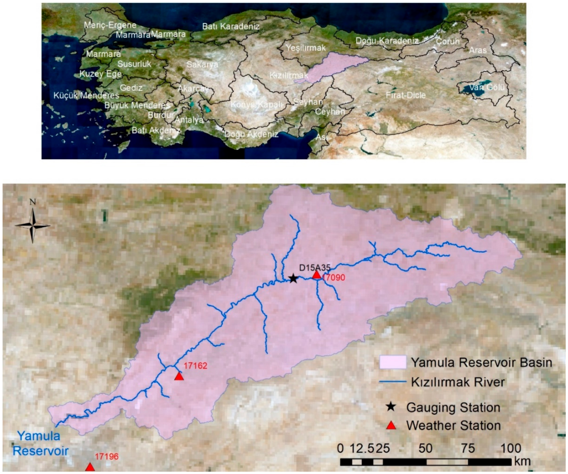
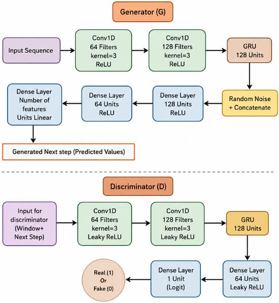
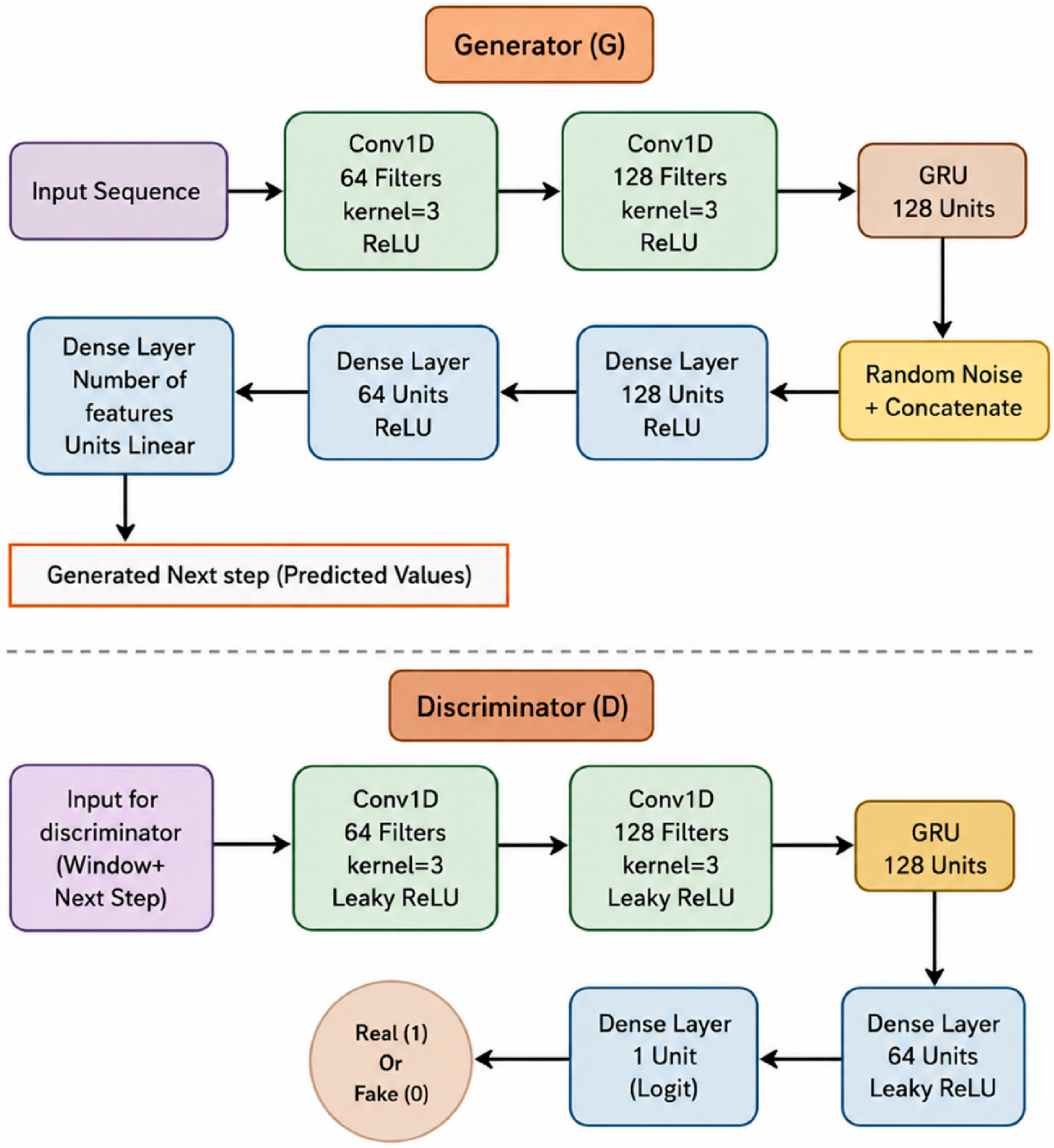
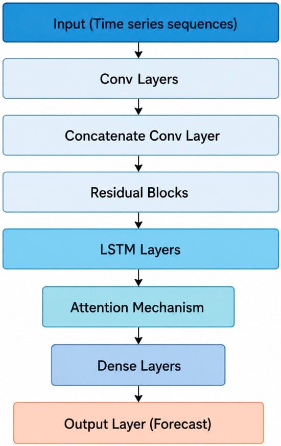
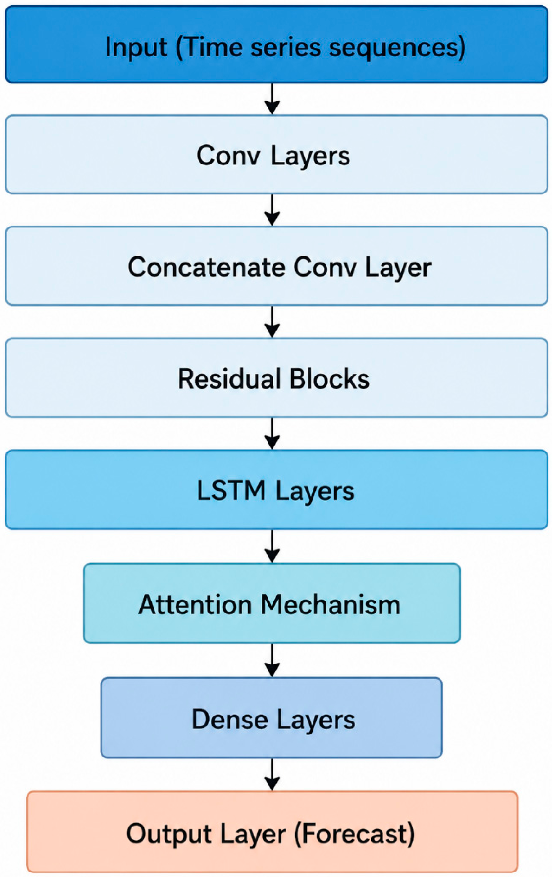
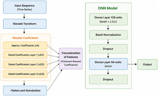
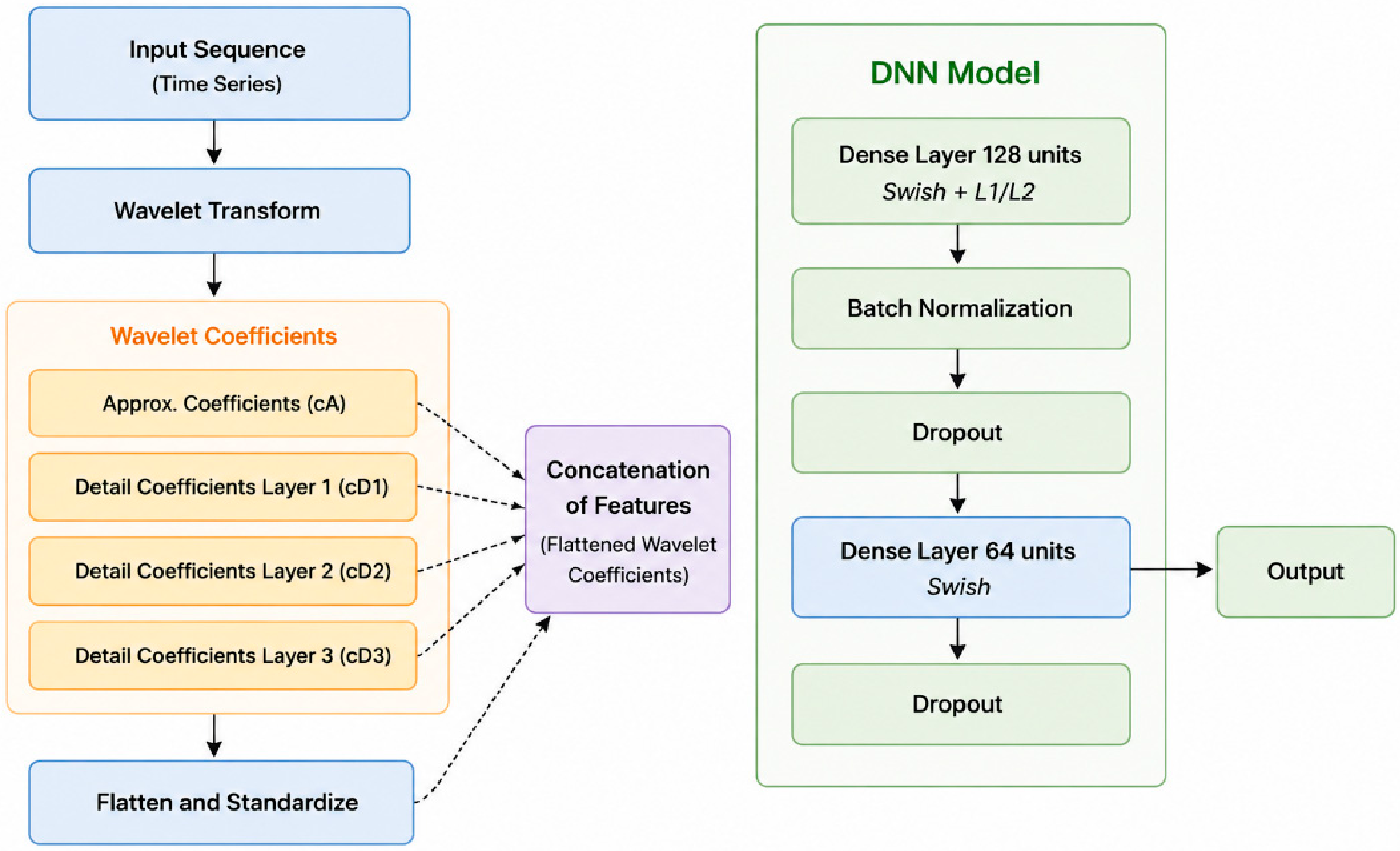
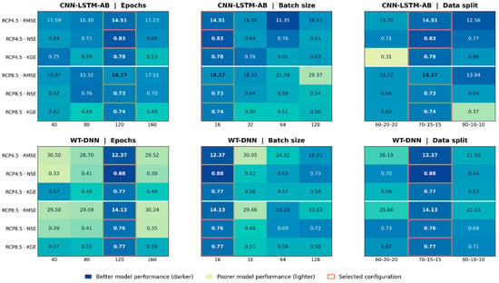
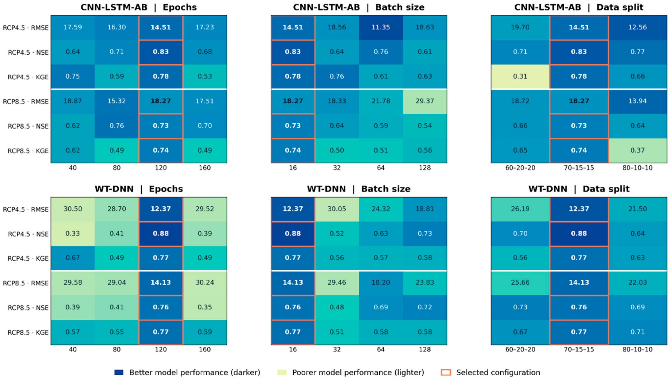
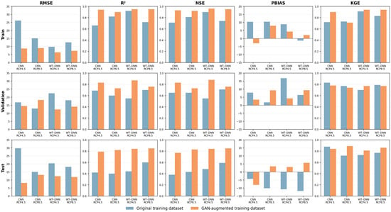
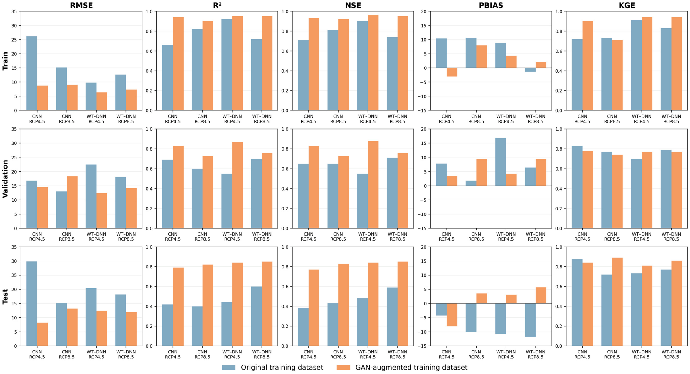
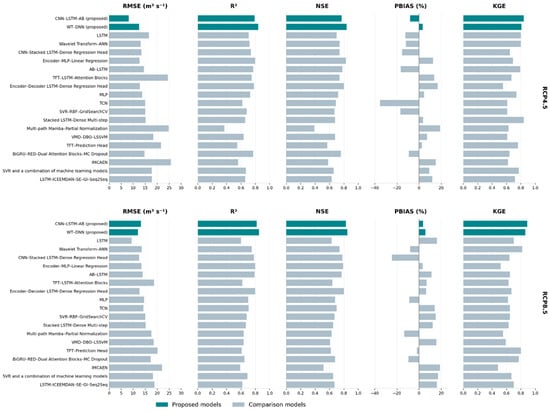
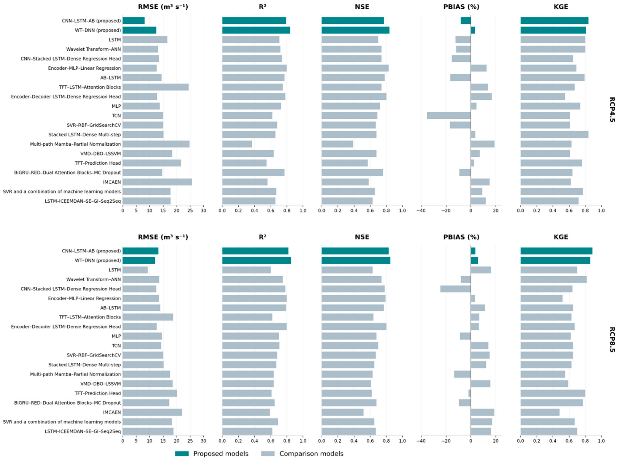
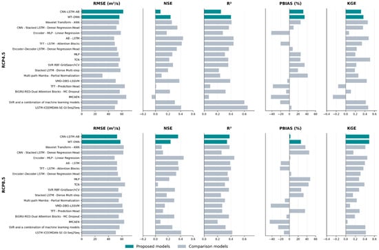
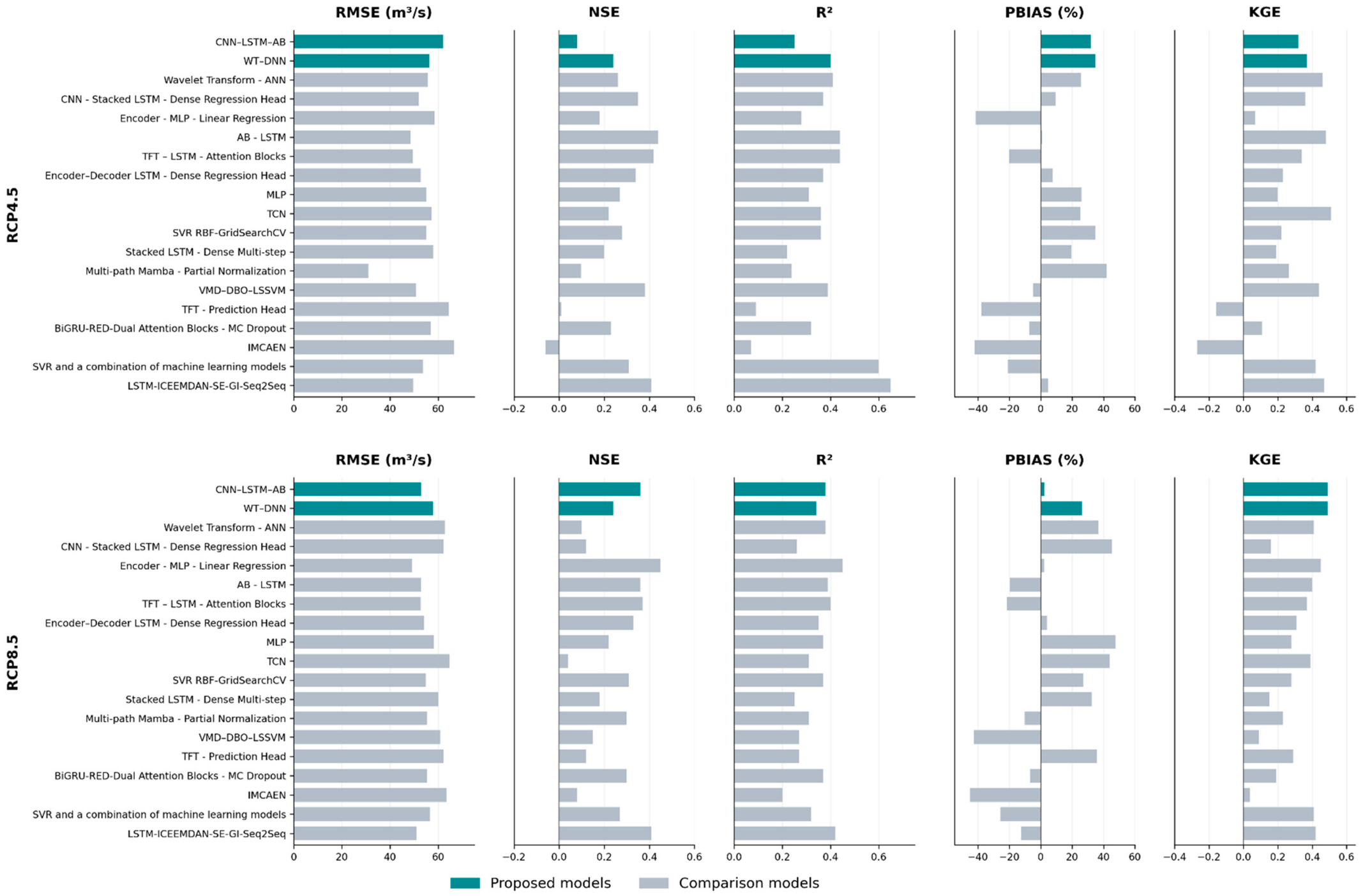

Disclaimer/Publisher’s Note: The statements, opinions and data contained in all publications are solely those of the individual author(s) and contributor(s) and not of MDPI and/or the editor(s). MDPI and/or the editor(s) disclaim responsibility for any injury to people or property resulting from any ideas, methods, instructions or products referred to in the content. |
© 2026 by the authors. Licensee MDPI, Basel, Switzerland. This article is an open access article distributed under the terms and conditions of the Creative Commons Attribution (CC BY) license.