


Abstract
Agricultural drainage discharges into coastal waters whose nutrient concentrations also respond to ocean circulation and internal biogeochemical cycling. We analysed 48 monthly Copernicus Marine surface records per sector from January 2022 to December 2025 along the Lambayeque coast, Peru. All nitrate, carbon and oxygen relationships derive from one numerical modelling framework without independent contemporaneous local validation. Two distinct model series represented northern and southern receiving-water sectors adjacent to four drain outlets. Nitrate averaged 10.672 ± 2.623 and 12.210 ± 2.906 mmol m−3, respectively, and remained higher in the south in all 48 paired months. Both sectors showed enrichment during May–October. After removing calendar-month means, nitrate remained positively correlated with dissolved inorganic carbon (r = 0.812 north and 0.908 south) and inversely correlated with oxygen (r = −0.678 and −0.784), with nominal month-adjusted p < 0.001 for all four associations. Block-bootstrap intervals and resampling with re-estimated seasonal means retained these directions. Reproduced four-point agricultural relationships supplied ancillary context. The results identify persistent receiving-water contrasts and covariance beyond the mean seasonal cycle within the product. They support coordinated drainage and coastal monitoring rather than source attribution.
1. Introduction
Nitrogen management in irrigated landscapes requires attention to the waters receiving agricultural drainage as well as the fields where fertilisers are applied. Nitrate is readily transported through drainage and groundwater pathways, but downstream concentrations integrate water movement, dilution, biological uptake and transformation. The amount reaching a receiving water therefore depends on both nitrogen availability and hydrological connectivity. Research on drainage catchments and seasonal nitrate export shows that concentration, discharge and transport timing provide distinct information about nutrient delivery [1,2]. At coastal outlets, this catchment signal enters a water body with its own circulation and biogeochemical cycle. A nitrate concentration measured or modelled near an outlet cannot, by itself, identify an agricultural source or quantify its contribution.
The distinction is particularly relevant along eastern boundary upwelling margins. Along the Peruvian coast, wind-driven upwelling introduces subsurface waters into the upper ocean, while mixing, biological assimilation, remineralisation and nitrogen removal modify the resulting nutrient distributions [3,4,5]. Oxygen conditions further influence nitrogen transformations [6]. Terrestrial inputs can modify coastal chemistry, as documented in other coastal settings, but their influence must be assessed against the marine background [7]. For catchment-to-coast water-quality assessment, the first task is consequently to characterise receiving-water variability at a spatial scale supported by the available evidence, before interpreting a concentration difference as a drainage impact.
A multivariable approach helps describe this background. Dissolved inorganic carbon (DIC), total alkalinity and the surface partial pressure of carbon dioxide (pCO2) characterise different aspects of the carbonate system. Chlorophyll a, phytoplankton carbon and net primary production (NPP) describe biomass-related properties or production, whereas dissolved oxygen reflects the balance among physical supply, solubility, photosynthesis and respiratory consumption. Their joint variation with nitrate helps identify recurring environmental states, although it does not isolate the processes producing them. Hydrodynamic transport and residence time influence nitrogen distributions and removal [8], while nutrient enrichment, carbon chemistry and oxygen loss interact in coastal upwelling systems [9,10]. Joint nutrient and plankton assessment also improves interpretation of eutrophication responses relative to a nutrient-only approach [11].
Operational marine products offer temporally regular information where coastal monitoring is sparse. The Copernicus Marine Global Ocean Biogeochemistry Analysis and Forecast product supplies co-located fields from a common modelling framework [12]. This consistency facilitates temporal matching and comparison between sectors. It also creates an interpretative constraint: variables share model structure, physical forcing and parameterised biological processes [13]. Correlations among such fields describe internal model covariance and cannot serve as independent validation of environmental coupling. Other marine information systems, including regional reanalyses, operational ocean-colour products and integrated buoy–satellite programmes, illustrate complementary approaches to assessing coastal variability [14,15,16]. These approaches differ in observational support, resolution and purpose and do not validate the specific Lambayeque extractions used here.
The Lambayeque coast receives drainage from an irrigated agricultural plain where rice production and nitrogen fertiliser supply provide relevant land-management context. Studies of rice systems show that fertiliser placement, water management and application practices affect nitrogen losses [17,18,19]. Environmental assessments likewise depend on management practices and the boundaries of the production system [20]. Lambayeque rice production and national urea imports indicate agricultural output and fertiliser availability at different spatial scales. They do not measure nitrogen applied within a drain catchment. Their comparison with coastal concentrations is therefore ancillary to the monthly receiving-water analysis.
The objective of this study is to assess seasonal nitrate variability and nitrate–carbon–oxygen covariability in two Copernicus Marine surface series off Lambayeque during 2022–2025. The contribution is a reproducible assessment of modelled receiving-water conditions that supplies spatial and seasonal hypotheses for independent field testing. We quantify the paired contrast between the two series, distinguish mean seasonality from interannual anomalies and test the sensitivity of associations to analytical choices. Four annual agricultural pairs provide contextual comparisons. The hydrological application is to specify where and when concurrent drainage-discharge and coastal observations should be collected. The study describes receiving-water concentrations, not measured catchment export or land–sea transport.
2. Materials and Methods
2.1. Study Area, Spatial Support and Analytical Design
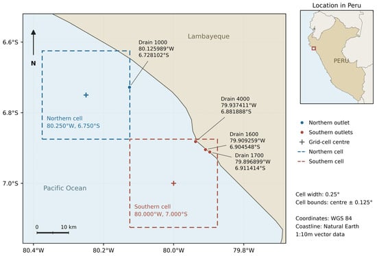
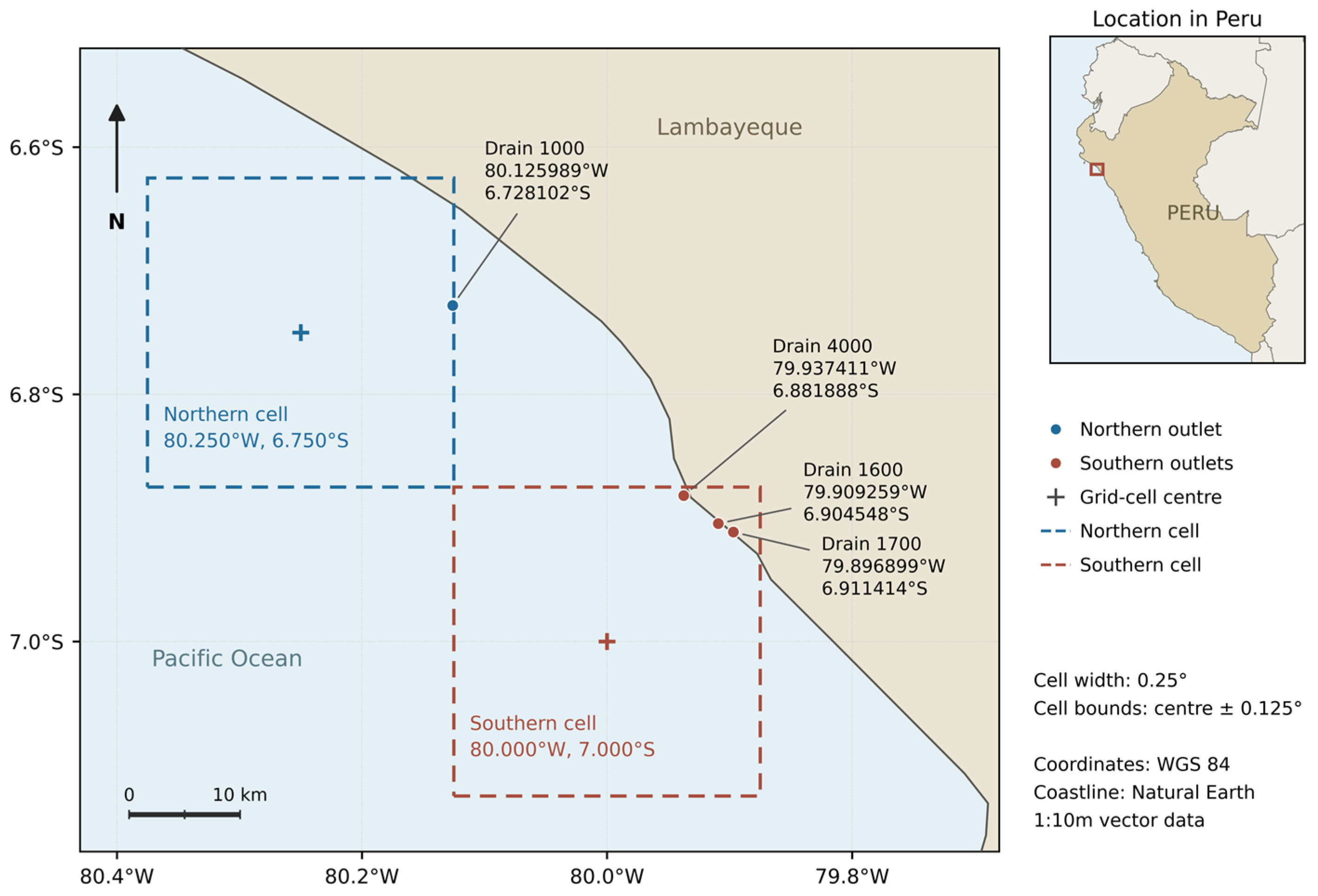
The study used a retrospective analysis of monthly surface biogeochemical fields for January 2022 to December 2025. The northern sector was associated with the Drain 1000 outlet, located at 80.125989° W and 6.728102° S. The southern sector was associated with drains 1600, 1700 and 4000, with outlet coordinates of 79.909259° W and 6.904548° S, 79.896899° W and 6.911414° S, and 79.937411° W and 6.881888° S, respectively. These coordinates identify drainage outlets rather than in situ marine sampling stations. The study compares modelled receiving-water conditions adjacent to these locations (Figure 1).
Figure 1.
Reported drain outlets and surface Copernicus Marine grid support along the Lambayeque coast, Peru. Dashed outlines show nominal 0.25° cells centred at 80.250° W, 6.750° S (north) and 80.000° W, 7.000° S (south), using the accompanying grid metadata. Crosses mark cell centres and circles mark the reported outlets. Cell bounds are centre ± 0.125°. The coastline and country boundaries are generalised from Natural Earth 1:10 m vector data [21]. The scale bar refers to the main map. Coordinates use WGS 84. Leader lines link labels to points and do not represent drainage channels or transport pathways.
The archived CSV files record extraction request points that differ slightly from the outlet coordinates. The northern request point was 80.125634° W and 6.722697° S. The primary southern series used the Drain 1700 request point at 79.891101° W and 6.915135° S. The three southern extractions yielded the same time series within decimal export precision and were retained once. They do not provide three independent marine replicates. The accompanying grid metadata report two wet-cell centres: 80.250° W, 6.750° S in the north and 80.000° W, 7.000° S in the south, with index pairs (i, j) of (399, 293) and (400, 292). Reported bottom depths are 23.335 and 31.835 m, respectively, and both marine-mask values are 1. Table 1 separates outlet, request and cell-centre coordinates. The archived CSV files do not independently encode the returned grid indices, and the original gridded file and index-origin convention were not retained. The mapped centres therefore follow the accompanying metadata rather than a new retrieval from the historical gridded product.
Table 1.
Outlet, CSV request and reported marine cell-centre coordinates, WGS 84.
The two unique series are the spatial units of the analysis. Repeated monthly values describe temporal variation within each unit and do not increase spatial replication. At this latitude, the nominal grid spacing is approximately 28 km, much larger than an individual drainage outlet. The sector labels therefore denote coastal model support rather than catchment boundaries, plume limits or homogeneous water-quality zones. The analytical design supports assessment of sectoral contrasts within the product, but not extrapolation to every location along the Lambayeque shoreline.
2.2. Marine Product, Variables and Units
The marine data originate from the Copernicus Marine Global Ocean Biogeochemistry Analysis and Forecast product, GLOBAL_ANALYSISFORECAST_BGC_001_028, DOI 10.48670/moi-00015 [12]. The extraction documentation identifies the monthly P1M-m datasets and Product User Manual Issue 1.4, November 2025 [22]. This manual describes monthly means from the previous month’s best-analysis fields. We used the archived monthly values directly, without averaging daily forecasts. All selected filenames encode export timestamps on 15 January 2026, between 02:30:03 and 04:25:13 UTC. Older northern exports encode 26 March 2025. These timestamps identify the archived exports, not the production release of each field. No separate dataset release tag was retained, and the manual issue is not treated as that tag. The PISCES framework links nutrient, carbon and biological dynamics [13]. These records are model outputs, not direct drain-outlet measurements.
Nitrate was the focal state variable. Seven companion variables were specified before the correlation analysis: total alkalinity, DIC, surface pCO2, chlorophyll a, phytoplankton carbon, NPP and dissolved oxygen. Table 2 gives the dataset components, native variable names and units. All three-dimensional variables refer to the shallowest archived layer, centred at approximately 0.4940254 m below the surface. Surface pCO2 is a two-dimensional field without a depth dimension. Units were retained as exported. NPP is a volumetric production rate and was not treated as standing phytoplankton biomass. Archived phosphate and pH values are retained in the analytical archive for completeness, but they were not added to the seven-variable primary correlation family.
Table 2.
Marine variables, native product units and monthly dataset components.
Product-level validation against ocean-colour observations, biogeochemical floats and climatologies is documented by Copernicus [23,24]. These assessments do not establish accuracy at the two Lambayeque cells. Independent historical context comes from IMARPE’s June 2017 coastal survey [25], which predates the study period and differs in depth, spatial support and sampling frequency. No contemporaneous, co-located field series was available for validation.
2.3. Archive Harmonisation and Quality Control
Source files were inventoried by drain, variable, native field, depth, units, temporal coverage and filename timestamp. We selected the latest internally consistent CSV export set, confirmed complete 2022–2025 coverage, and checked southern duplication before joining variables. The author-confirmed supplementary workbook reproduces all 960 selected biogeochemical values to numerical precision. Historical spreadsheet compilations were assessed separately, with record-level differences and summary metrics reported in the Supplementary Materials. They were not mixed with the selected exports. For nitrate, 14 of 48 monthly values differ by more than 10−6 mmol m−3 in each primary sector. The mean absolute CSV–historical-workbook differences are 0.205 mmol m−3 in the north and 0.161 mmol m−3 in the south, with maxima of 2.437 and 1.574 mmol m−3. The affected nitrate months are November 2023–December 2024. The source inventory and SHA-256 checksums preserve the provenance of each representation. Selection reflects consistent provenance and coverage, not an assumption that a later export is more accurate.
Dates, decimal separators, units, depth and duplicate values were checked before joining variables by calendar year and month. Three records from October–December 2021 were excluded to maintain the specified study period. The selected CSV files contained January–December values in all four study years for both sectors. Each sector therefore contributed 48 monthly observations, with 12 values in every annual analysis. No monthly value was imputed. Agreement among the southern series was checked across the three outlet extractions before selecting one series, preventing repeated representations of the same model output from inflating the sample size.
Annual nitrate means were calculated from all 12 monthly values, and the four-year calendar-month means from four values per month. Standard deviations describe temporal variation in the model series. Sectoral differences were paired by month. Harmonisation preceded the statistical analysis. The supplementary tables in Supplementary File S1 provide the complete annual inputs and monthly series used in the revised analyses.
2.4. Ancillary Agricultural Indicators
Annual paddy-rice production in Lambayeque was obtained from MIDAGRI’s Observatorio de Commodities Arroz N.° 01-2026, Table 8, p. 26 [26]. Annual imports of urea for agricultural use across Peru were obtained from El Agro en Cifras, December 2025, Table C.90, pp. 134–135, which credits SUNAT [27]. For 2022, 2023, 2024 and 2025, rice production was 440,156, 406,891, 509,895 and 471,203 t, and national urea imports were 330,287, 255,559, 441,871 and 356,378 t. These published annual totals reproduce the author-confirmed workbook. The exact editions are specified because earlier publications contain different annual figures. Each annual nitrate mean uses January–December values from the selected CSV series. All three annual relationships were recalculated from these four year-matched pairs.
Rice production describes harvested crop mass in Lambayeque, whereas urea imports describe national fertiliser supply. Imports do not establish allocation to Lambayeque, individual crops or drain catchments. The annual comparisons were retained to document these broad indicators alongside receiving-water conditions, with n = 4, two-sided nominal Pearson p-values and R2 from ordinary least-squares regression with an intercept. They are exploratory contextual summaries and do not estimate fertiliser application or nitrogen export.
2.5. Statistical Analysis and Temporal Dependence
Descriptive analysis first summarised nitrate by sector, year and calendar month (Figure 2 and Table 3). The contrast between sectors was expressed as the mean of the 48 paired monthly southern-minus-northern differences. May–October and November–April averages were reported as descriptive summaries of the seasonal pattern. These intervals were not selected as independently validated hydrological seasons or used to estimate a seasonal agricultural effect. The number of paired months with higher southern nitrate and the correlation between the two nitrate series were also recorded.
Figure 2.
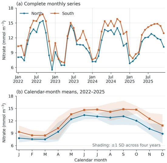
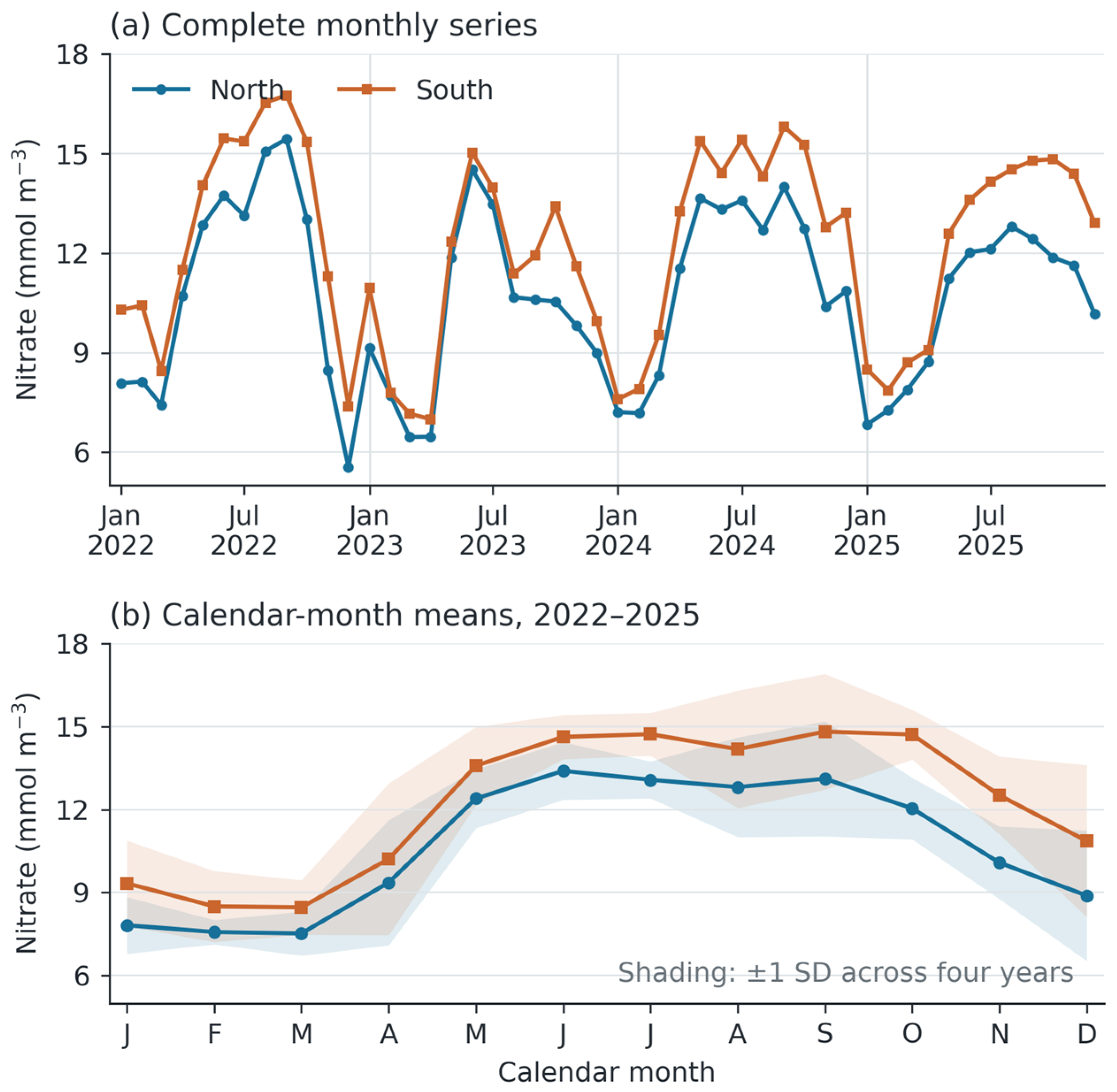
Monthly surface nitrate concentration in the northern and southern marine sectors, January 2022–December 2025. (a) Complete monthly series, with 48 values per sector. (b) Calendar-month means across four years, with shading indicating ±1 standard deviation among the four annual values for each month. The southern record represents the common series returned for the three southern outlet requests and enters the analysis once. Concentrations are expressed in mmol m−3.
Table 3.
Annual surface nitrate summaries (a) and pooled surface oxygen summaries (b).
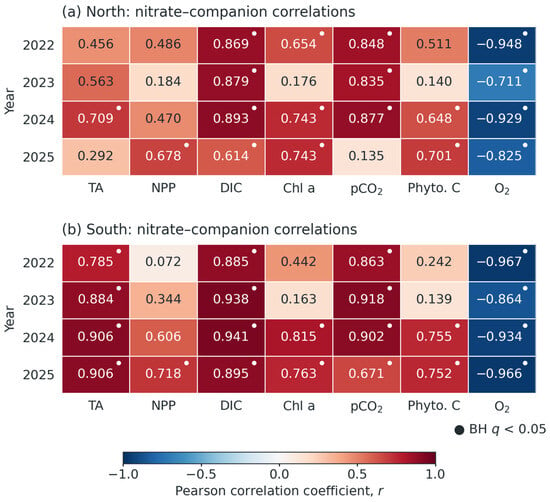
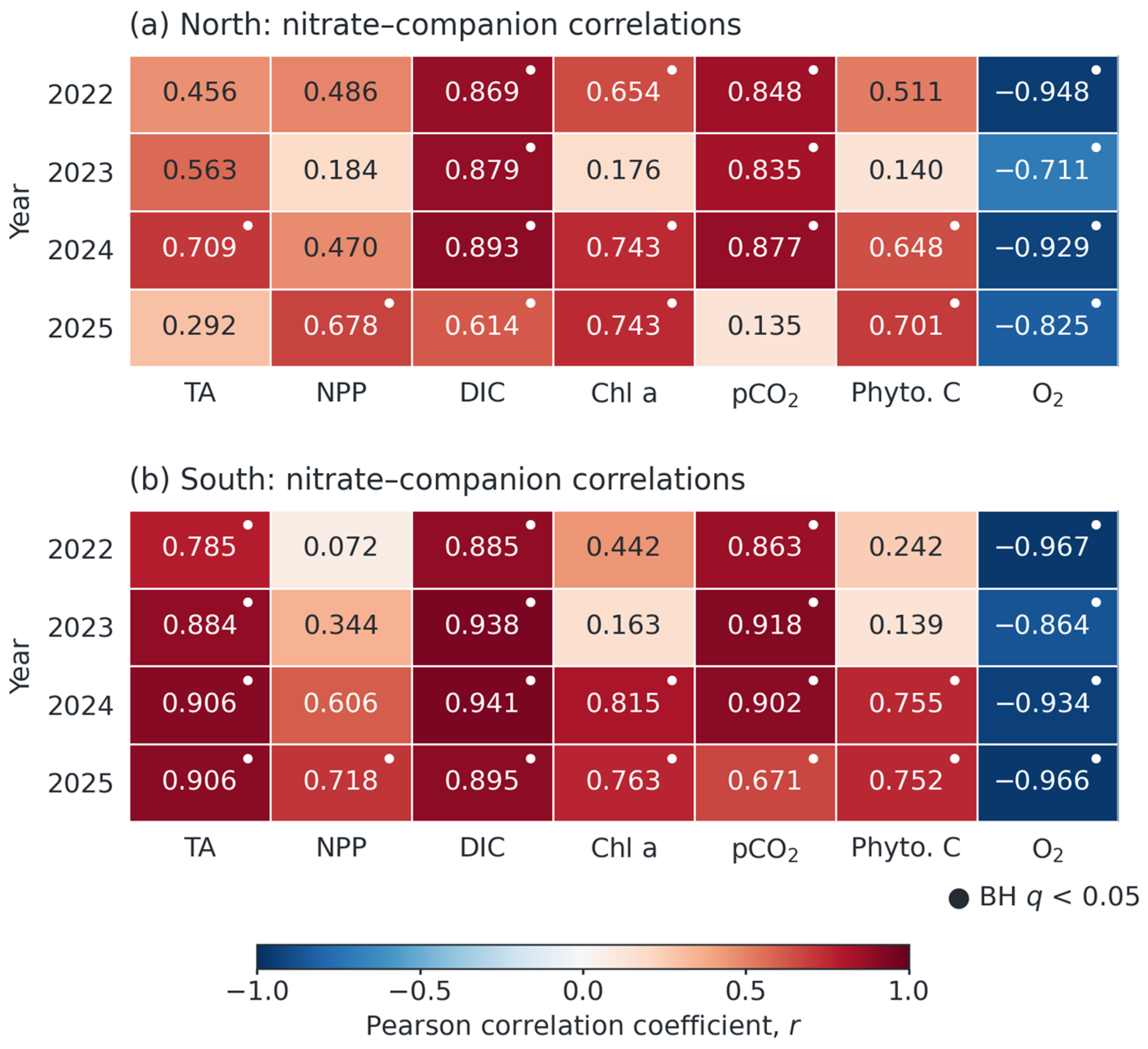
Within each sector and year, Pearson coefficients described nitrate associations with seven companion variables using 12 monthly pairs. The family comprised 56 comparisons. Two-sided nominal p-values were adjusted using the Benjamini–Hochberg procedure [28], with seven-comparison sector–year adjustments also supplied. We additionally assessed serial dependence using the lag-one approximation ne = n(1 − ρxρᵧ)/(1 + ρxρᵧ), capped at n, where ρx and ρᵧ are the lag-one autocorrelations [29]. Approximate probabilities use ne − 2 degrees of freedom only when ne > 2. Tests with ne ≤ 2 remain unestimable. For the diagnostic BH calculation, their positions are retained in the 56-test family using 1 for ranking only, while their reported p- and q-values remain unavailable. Given the short seasonal series, this AR(1)-based calculation is a diagnostic, not a calibrated replacement test. The complete coefficients, nominal probabilities, effective sample sizes and multiplicity adjustments appear in Within_year.csv. Figure 3 retains nominal markers as descriptive information.
Figure 3.
Within-year Pearson correlations between surface nitrate and seven companion variables in (a) the northern and (b) the southern marine sector. Each cell reports r from 12 monthly pairs. Small dots indicate nominal Benjamini–Hochberg q < 0.05 across 56 comparisons, without adjustment for temporal dependence. Complete p-values, q-values and the lag-one sensitivity are supplied in Within_year.csv. The figure describes covariance among fields generated by a shared model and does not establish independent environmental coupling. TA, total alkalinity. NPP, net primary production. DIC, dissolved inorganic carbon. Chl a, chlorophyll a. pCO2, surface partial pressure of carbon dioxide. Phyto. C, phytoplankton carbon. O2, dissolved oxygen.
To distinguish mean seasonality from departures around it, calendar-month anomalies were calculated separately for every variable and sector: X′(y,m) = X(y,m) − X−(m), where X−(m) is the mean across 2022–2025 for month m. This four-observation monthly reference is an internal seasonal cycle, not a long-term climatology. Correlations across the 48 paired anomalies were compared with raw monthly correlations. Nominal anomaly p-values account for the 11 calendar-month contrasts, using 35 residual degrees of freedom. They still assume independent residuals. Block resampling supplies a separate dependence sensitivity. Seasonal removal does not establish independence from common physical forcing.
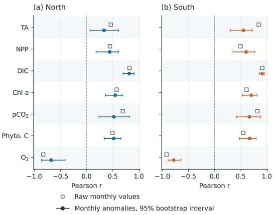
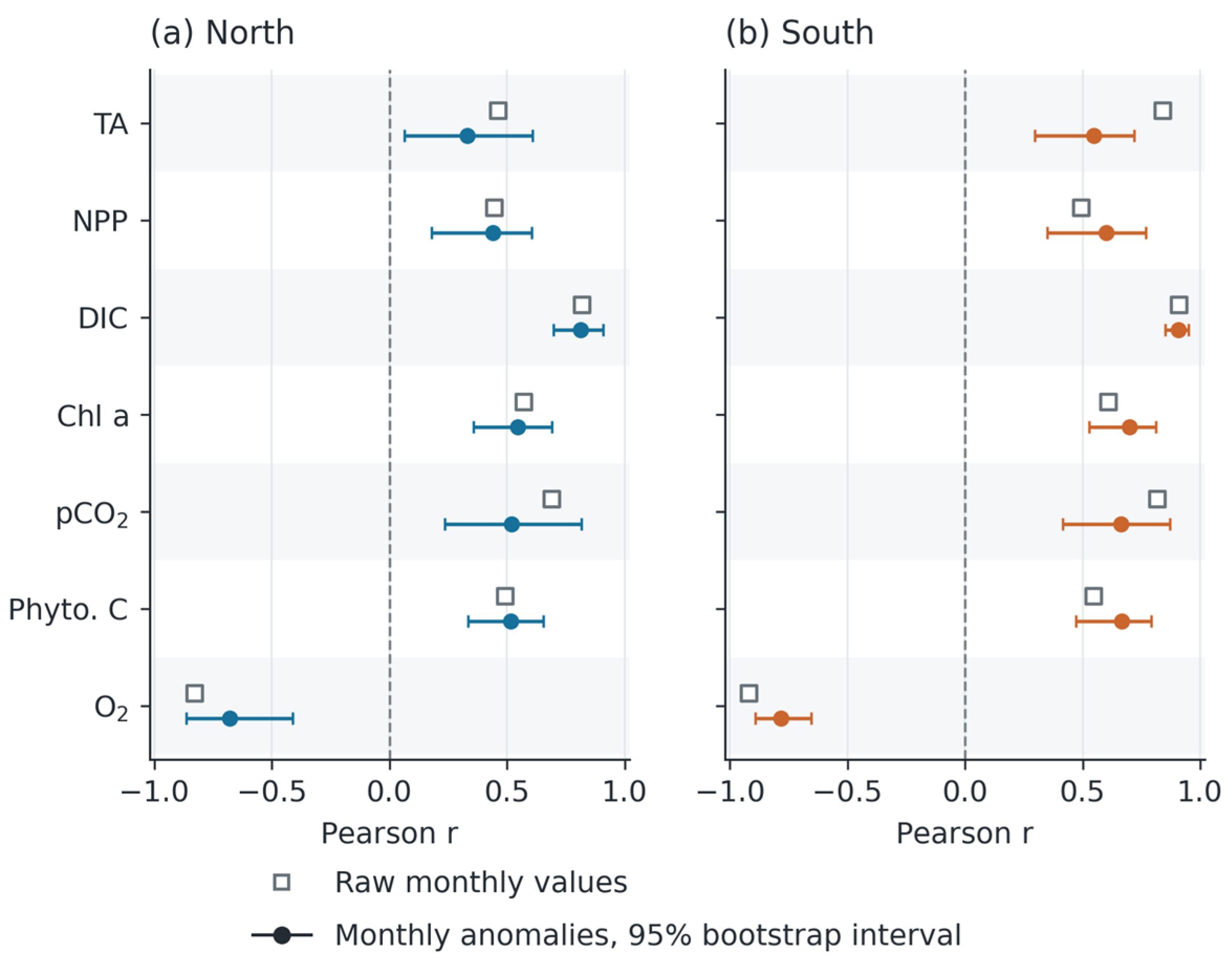
Paired circular moving-block bootstrap resampling preserved consecutive paired observations within each block [30]. The principal analysis used six-month blocks, 10,000 replicates and seed 20261006. Six months was chosen as an intermediate sensitivity scale between quarterly and annual blocks, not as an estimated optimum. Three- and twelve-month blocks tested dependence-span sensitivity. Percentile intervals use the 2.5th and 97.5th percentiles. Figure 4 and Table 4 retain the principal intervals, and the Supplementary Material supplies independently regenerated intervals for all block lengths, with explicit seeds and sampling order. Small Monte Carlo differences between runs do not alter the signs. These intervals describe variation within the supplied series and do not quantify model structural error or extrapolation beyond the study period.
Figure 4.
Pooled nitrate–companion correlations before and after removal of the calendar-month means in (a) the northern and (b) the southern marine sector, with 48 paired months per sector. Open squares show correlations of raw monthly values. Filled circles show correlations of monthly anomalies, with 95% percentile intervals from 10,000 paired circular block-bootstrap samples using six-month blocks. Intervals condition on the four-year monthly climatology and quantify sampling variability within the supplied model series, excluding model and observational uncertainty. Variable abbreviations follow Figure 3.
Table 4.
Nitrate associations before and after removal of calendar-month means.
The principal anomaly bootstrap held the estimated calendar-month means fixed. To assess sensitivity to this seasonal reference, we also enumerated all 256 ordered selections of four complete years with replacement and re-estimated the 12 monthly means in each selection. Four selections containing a single repeated year produced zero anomalies and were excluded, leaving 252 valid selections. Their percentile ranges are short-record sensitivity summaries, not precise coverage guarantees. Additional checks comprised Spearman correlations, joint removal of month effects and a linear time term, and leave-one-year-out correlations with seasonal means recalculated from the three retained years. Complete results for all 14 associations are supplied in Block_bootstrap_sensitivity.csv, Reestimated_seasonal_bootstrap.csv, Detrend_rank_sensitivity.csv and Leave_one_year_out.csv.
The supplementary workbook also supplies monthly potential temperature, practical salinity and 10 m wind speed and components for both sectors. Their original product and extraction metadata were not retained, so we used them as diagnostic covariates, not independent observational validation. We compared seasonal means and residual correlations after removing temperature and salinity, then wind components, with and without calendar-month effects. Nominal partial-correlation probabilities use the residual design rank. A separate carbonate sensitivity multiplied volumetric DIC and alkalinity by 35/S, where S is practical salinity. This zero-freshwater-endmember scaling is not density normalisation. Full specifications and results appear in Hydrographic_sensitivity.csv, Physical_context.csv and Salinity_normalisation.csv.
The reproducible workflow used Python 3.12.14, NumPy 2.3.5, pandas 2.2.3 and SciPy 1.17.0. The Supplementary Materials contain the original source files, analysis-ready tables, software versions, source checksums and executable Python code. No monthly observation was generated or imputed.
3. Results
3.1. Completeness and Paired Sectoral Nitrate Contrast
The harmonised dataset contained 48 monthly records for each of two unique sectors, with complete nitrate and companion-variable coverage. The three southern outlet extractions agreed within export precision. Across January 2022–December 2025, mean nitrate was 10.672 ± 2.623 mmol m−3 in the north and 12.210 ± 2.906 mmol m−3 in the south. The observed monthly ranges were 5.542–15.435 and 6.994–16.751 mmol m−3, respectively. These standard deviations and ranges describe variation among monthly model values.
Southern nitrate exceeded northern nitrate in all 48 paired months. The mean paired difference was 1.538 mmol m−3, with a six-month block-bootstrap 95% interval of 1.204–1.870 mmol m−3. Independently regenerated three-, six- and twelve-month intervals remained above zero. The two nitrate series tracked one another closely (r = 0.965, nominal p < 0.001), showing a shared temporal pattern superimposed on a persistent sectoral offset. This result concerns the two model support locations.
Annual nitrate means varied from 10.019 to 11.288 mmol m−3 in the northern sector and from 11.039 to 12.907 mmol m−3 in the southern sector (Table 3a). Both sectors had their lowest annual mean in 2023 and their highest in 2024. The annual means did not increase monotonically and provide period-specific receiving-water context rather than evidence of a trend in nutrient loading.
3.2. Seasonal Structure and Timing
Figure 2 shows a broad seasonal increase during May–October in both sectors. Over the four-year record, northern mean nitrate was 12.805 mmol m−3 during May–October and 8.538 mmol m−3 during November–April. Corresponding southern means were 14.440 and 9.980 mmol m−3. The four-year calendar-month minimum occurred in March in both sectors, at 7.519 mmol m−3 in the north and 8.463 mmol m−3 in the south. The northern calendar-month maximum occurred in June, at 13.397 mmol m−3, whereas the southern maximum occurred in September, at 14.815 mmol m−3.
Individual years differed from the average cycle. Both sectors peaked in September 2022, June 2023 and September 2024. In 2025, the northern peak occurred in August and the southern peak in October. Thus, the recurring signal was a broad period of mid- to late-year enrichment rather than a fixed peak month. The southern series also retained higher calendar-month means towards the end of the year. These features identify a monitoring window but do not distinguish drainage seasonality from upwelling, mixing or biological demand.
3.3. Within-Year Nitrate Associations
The northern sector showed positive nitrate–DIC correlations in each year (r = 0.614–0.893, nominal p = 0.000093–0.0337, Figure 3). Nitrate–pCO2 correlations were positive during 2022–2024 (r = 0.835–0.877, p = 0.000183–0.000715), but weakened in 2025 (r = 0.135, p = 0.676). Nitrate–oxygen correlations remained negative (r = −0.948 to −0.711, p = 0.0000028–0.00955). Alkalinity associations varied more strongly (r = 0.292–0.709, p = 0.00981–0.357). These probabilities are nominal and require the dependence assessment below.
The southern sector displayed positive nitrate associations with alkalinity (r = 0.785–0.906, nominal p = 0.0000482–0.00249), DIC (r = 0.885–0.941, p = 0.00000523–0.000130) and pCO2 (r = 0.671–0.918, p = 0.0000256–0.0169). Oxygen correlations remained negative (r = −0.967 to −0.864, p = 0.000000297–0.000287). These ranges describe the individual sector records and are not a formal comparison of coupling strength between sectors.
Biological associations varied among years. Northern nitrate–chlorophyll a correlations were 0.654 (p = 0.0212) in 2022, 0.176 (p = 0.585) in 2023, 0.743 (p = 0.00561) in 2024 and 0.743 (p = 0.00564) in 2025. Northern phytoplankton-carbon coefficients were 0.140 (p = 0.664), 0.648 (p = 0.0227) and 0.701 (p = 0.0112) in 2023–2025. Corresponding southern chlorophyll a coefficients were 0.163 (p = 0.612), 0.815 (p = 0.00125) and 0.763 (p = 0.00386), and phytoplankton-carbon coefficients were 0.139 (p = 0.668), 0.755 (p = 0.00452) and 0.752 (p = 0.00479). NPP associations were also larger in 2025 than in 2023. These nominal comparisons describe interannual variability rather than a constant biological response to nitrate.
Across the 56 within-year comparisons, 39 nominal Benjamini–Hochberg q-values were below 0.05. The lag-one diagnostic reduced effective sample sizes to 1.04–9.62. Fifteen comparisons had ne ≤ 2 and no estimable adjusted probability, and none of the estimable comparisons retained q < 0.05 under the diagnostic adjustment. Thus, the dots in Figure 3 should not be interpreted as evidence robust to serial dependence. The multiyear anomaly and block-resampling results provide the more informative persistence assessment. All probabilities and effective sample sizes are reported in Within_year.csv.
3.4. Associations Beyond the Mean Seasonal Cycle
Removing calendar-month means reduced some associations but preserved their direction (Figure 4 and Table 4). Nitrate–DIC coefficients changed from 0.819 to 0.812 in the north and from 0.912 to 0.908 in the south (all nominal p < 0.001). Principal six-month bootstrap intervals for anomaly correlations were 0.698–0.908 and 0.851–0.951. Nitrate–oxygen coefficients weakened from −0.828 to −0.678 in the north and from −0.917 to −0.784 in the south (all nominal p < 0.001), with anomaly intervals of −0.864 to −0.411 and −0.892 to −0.655. The mean seasonal cycle therefore accounted for part, but not all, of the nitrate–oxygen association within the product.
Anomaly correlations with pCO2 were 0.518 in the north (nominal month-adjusted p = 0.00101) and 0.663 in the south (p < 0.001), compared with raw coefficients of 0.691 and 0.818 (both p < 0.001). Alkalinity coefficients decreased from 0.463 (p < 0.001) to 0.332 (p = 0.0446) in the north and from 0.839 (p < 0.001) to 0.548 (p < 0.001) in the south. Biological anomaly correlations remained positive: NPP, chlorophyll a and phytoplankton carbon were 0.438 (p = 0.00664), 0.546 (p < 0.001) and 0.516 (p = 0.00108) in the north, and 0.601, 0.698 and 0.666 in the south (all p < 0.001). Fixed-reference intervals for all 14 associations retained their sign across three-, six- and twelve-month block lengths.
The principal DIC and oxygen associations were not dependent on a single year. Leave-one-year-out anomaly coefficients ranged from 0.758 to 0.864 for DIC in the north and from 0.853 to 0.939 in the south (all nominal month-adjusted p < 0.001). Oxygen ranges were −0.819 to −0.466 and −0.815 to −0.748, respectively (nominal month-adjusted p < 0.02 in the north and p < 0.001 in the south). Complete probabilities appear in Leave_one_year_out.csv. Spearman and detrended results retained the same directions. Re-estimating seasonal means in the year-resampling analysis yielded DIC percentile ranges of 0.692–0.903 and 0.835–0.969, and oxygen ranges of −0.854 to −0.326 and −0.840 to −0.734. Northern alkalinity (−0.172 to 0.623) and NPP (−0.018 to 0.707) included zero in this analysis. Persistence therefore differs among variables and cannot be generalised to every carbonate or biological association.
The historical spreadsheet representation retained the principal anomaly directions. Nitrate–DIC coefficients were 0.782 in the north and 0.894 in the south, compared with 0.812 and 0.908 for the selected CSV series. Oxygen coefficients were −0.702 and −0.791, compared with −0.678 and −0.784. All eight coefficients have nominal month-adjusted p < 0.001. These comparisons assess input-representation sensitivity, not model accuracy. Record-level differences and complete variable summaries are provided in CSV_workbook_pointwise_differences.csv and CSV_workbook_differences.csv.
3.5. Ancillary Annual Agricultural Summaries
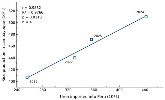
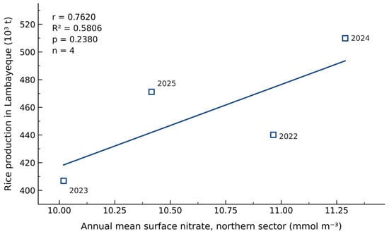
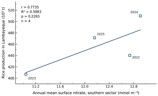
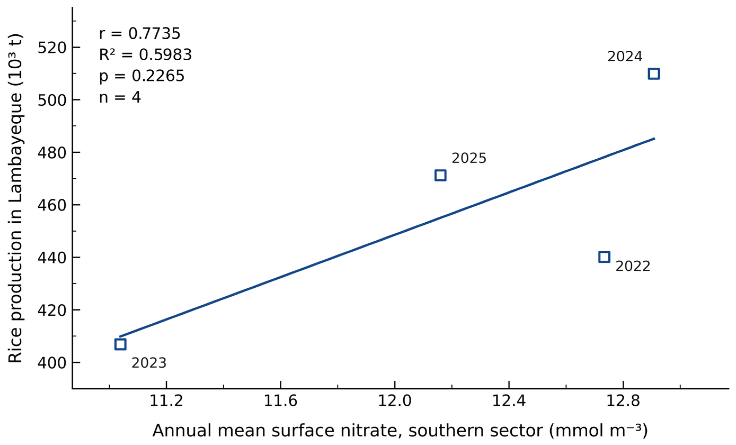
Using the verified annual inputs, rice production and national urea imports were positively associated (r = 0.988, R2 = 97.66%, n = 4, nominal p = 0.0118, Figure 5). Rice–nitrate coefficients were 0.762 in the north (R2 = 58.06%, p = 0.238) and 0.774 in the south (R2 = 59.83%, p = 0.226), each with four annual pairs (Figure 6 and Figure 7, Table 5). The latter two associations were not distinguishable from zero under the conventional two-sided test. All three figures use the same year-labelled source table, and the nitrate values match the complete-year means in Table 3.
Figure 5.
Association between Lambayeque paddy-rice production and national imports of urea for agricultural use in Peru, 2022–2025. Points identify the four calendar years. The line is an ordinary least-squares fit with an intercept. r = 0.988, R2 = 97.66%, n = 4 and nominal two-sided p = 0.0118. Source values: MIDAGRI [26,27], with SUNAT credited for imports. Different spatial supports and four observations limit inference about local fertiliser use.
Figure 6.
Association between Lambayeque paddy-rice production and complete-year mean surface nitrate in the northern marine sector, 2022–2025. Points identify the four calendar years. The line is an ordinary least-squares fit with an intercept. r = 0.762, R2 = 58.06%, n = 4 and nominal two-sided p = 0.238. Rice values follow MIDAGRI [26], and nitrate means use all 12 selected monthly values per year.
Figure 7.
Association between Lambayeque paddy-rice production and complete-year mean surface nitrate in the southern marine sector, 2022–2025. Points identify the four calendar years. The line is an ordinary least-squares fit with an intercept. r = 0.774, R2 = 59.83%, n = 4 and nominal two-sided p = 0.226. Rice values follow MIDAGRI [26], and nitrate means use all 12 selected monthly values per year.
Table 5.
Recalculated annual agricultural relationships for 2022–2025.
The national urea–regional rice association describes co-variation between indicators with different spatial coverage. Its nominal p-value does not establish local fertiliser use or drainage delivery. With four successive annual pairs, all three fitted relationships remain sensitive to individual years and provide limited inferential support. Their purpose is to make the agricultural context reproducible and to define the scale of future catchment-specific comparisons. The small difference between the two rice–nitrate R2 values is not evidence of a sectoral difference in agricultural influence. These four-point fits establish neither stable agricultural relationships during 2022–2025 nor long-term coastal patterns, and non-significant rice–nitrate tests do not demonstrate the absence of agricultural influence.
4. Discussion
4.1. Receiving-Water Conditions at the Catchment-to-Coast Interface
The most direct result for water-quality assessment is the persistent nitrate difference between the two coastal model sectors. Southern values exceeded northern values in every matched month, yet both series shared a strong temporal pattern. A common regional influence combined with a sector-dependent offset is consistent with this structure. Drainage inputs, water-mass properties, bathymetry, circulation, mixing and biological processing are candidate contributors, rather than identified causes.
The receiving-water baseline supplies a temporal framework for concurrent drain measurements. Catchment studies evaluate export through the joint behaviour of concentration and discharge, with seasonal timing and transport pathways shaping loads [1,2]. Hydrodynamic controls on redistribution, residence time and removal then modify the relation between coastal concentration and source strength [8]. Paired sampling of both sides of this interface would connect the present coastal assessment to catchment hydrology.
Oxygen was lower in the south in all 48 paired months (Table 3b). Northern and southern means were 208.339 ± 12.910 and 193.554 ± 17.282 mmol m−3, respectively. The paired southern-minus-northern difference was −14.784 ± 9.011 mmol m−3, equivalent to −0.473 ± 0.288 mg L−1, with monthly differences ranging from −32.876 to −0.195 mmol m−3. This quantitative co-occurrence supports paired nutrient–oxygen monitoring, while its physical and ecological interpretation requires depth-resolved observations.
4.2. Seasonal Timing and Regional Marine Forcing
The broad May–October nitrate enhancement coincided with cooler, windier conditions in the supplementary physical series. Northern temperature averaged 18.63 °C in May–October and 20.94 °C in November–April, with wind speeds of 5.05 and 3.51 m s−1. Southern means were 18.35 and 20.67 °C, and 5.37 and 3.73 m s−1. Raw nitrate–temperature correlations were −0.650 and −0.776, and nitrate–wind-speed correlations were 0.685 and 0.630 (all nominal p < 0.001). These quantitative patterns are consistent with regional seasonal forcing discussed for the northern Humboldt system [3,5]. Wind speed is not an upwelling transport index, and the source-metadata limitations of the supplementary covariates prevent an independent process validation.
The different peak months among years also matter for monitoring design. A campaign confined to one nominal peak month would have missed the annual maximum in several sector–year combinations. Repeated observations spanning the broad enrichment period provide a more defensible representation of receiving-water conditions than a single annual visit. The March minimum in both four-year mean cycles offers a contrasting lower-nitrate period. Field comparisons should retain coverage outside May–October because transient drainage pulses, stratification changes and biological events can occur outside the modelled seasonal maximum.
Agricultural activity could overlap with the same seasonal marine cycle without being its cause. Irrigation schedules, fertiliser applications and drainage release would need to be resolved at the contributing catchment scale and matched to travel times. Rice-system studies demonstrate that nitrogen losses change with management practices [17,18,19], so a regional annual production value cannot substitute for this temporal detail. The present results therefore help select contrasting receiving-water conditions for sampling, while leaving the agricultural and marine components of seasonal nitrate unresolved.
4.3. Nitrate, Carbon Chemistry and Biological Response
Nitrate–DIC covariance persisted beyond the mean seasonal cycle and after individual years were excluded. Joint residualisation against calendar month, temperature, salinity and the eastward and northward wind components gave partial coefficients of 0.804 in the north and 0.838 in the south (nominal p < 0.001). Oxygen partial coefficients were −0.866 and −0.828 (nominal p < 0.001). These diagnostic results show persistence under the specified linear adjustments, not independence from physical forcing or shared model structure.
Upwelling, vertical mixing and remineralisation can jointly modify nutrient, carbon and oxygen fields [4,6,10]. The hydrographic sensitivity also shows why carbonate descriptors require separate interpretation. After a simple salinity scaling to 35, nitrate–DIC anomaly coefficients decreased to 0.428 in the north (nominal month-adjusted p = 0.00815) and 0.597 in the south (p < 0.001). Alkalinity coefficients changed to −0.266 (p = 0.112) and −0.222 (p = 0.186). This scaling assumes a zero freshwater endmember and does not convert volumetric concentrations to density-normalised concentrations. It therefore serves as a mixing sensitivity, not a complete carbonate-system correction. The persistence of DIC associations should not be extended to alkalinity.
The pCO2 relationship was less stable than the DIC relationship, particularly in the north in 2025. Surface pCO2 responds to temperature and the combined carbonate-system state. Residual correlations after adjustment for month, temperature, salinity and wind remained positive (north r = 0.788 and south r = 0.803, nominal p < 0.001), but this linear diagnostic is not a thermodynamic decomposition. The product quality overview reports positive pCO2 bias in eastern-boundary upwelling regions [24]. Co-located temperature, salinity, DIC and alkalinity measurements are needed to separate thermal, mixing and biological effects.
Biological fields provided a complementary but less uniform response. Higher nitrate did not correspond to equally strong NPP, chlorophyll a or phytoplankton-carbon associations in every year. Nutrient availability is one control on production and biomass, alongside light, mixing, residence time, grazing and other nutrient requirements. NPP and standing biomass also represent different parts of the biological response and need not covary identically. Work on remotely observed chlorophyll and operational ocean-colour variables illustrates the value of independent biological indicators [15,31]. Such observations could test whether the modelled Lambayeque biological anomalies coincide with coastal biomass changes.
4.4. Oxygen Covariation and Ecological Interpretation
The inverse nitrate–oxygen relationship recurred in all years and persisted after seasonal adjustment in both sectors. The reduction in its magnitude after removing calendar-month means indicates a seasonal contribution, while the remaining anomaly relationship indicates additional shared variation. Nutrient-rich, oxygen-poor waters supplied from below are one explanation. Respiratory processing of organic matter is another, potentially influenced by both marine production and land-derived material. Coastal deoxygenation studies show that oxygen and nitrogen dynamics interact through several pathways [6], and riverine organic matter can affect coastal oxygen through indirect processes [32].
The present analysis cannot distinguish these mechanisms because the primary biogeochemical variables originate from one model framework and are aggregated to monthly surface values. Coastal eutrophication studies demonstrate that external nutrient inputs can alter oxygen and carbon conditions [9], while work in coastal lagoons links nitrate enrichment to changes in nitrogen transformations and greenhouse-gas production [33]. These findings justify measuring relevant processes in Lambayeque, but their mechanisms and effect sizes cannot be transferred directly to this open-coast setting. No greenhouse-gas flux, respiratory rate or bottom-water oxygen record was analysed here.
Monthly surface oxygen ranged from 5.432 to 7.592 mg L−1 in the north and from 4.692 to 7.224 mg L−1 in the south. No monthly value fell below the conventional hypoxia comparator of 2 mg L−1, equivalent to 62.5 mmol m−3 [34]. This comparator is not a universal biological safety threshold. Monthly surface means cannot exclude short-lived events or bottom-water depletion. The June 2017 IMARPE survey recorded 2.20 mg L−1 at the intertidal Dren 4000 mouth, alongside salinity of 24.832 [25]. Those historical point observations illustrate nearshore heterogeneity but do not validate the 2022–2025 monthly cell series.
4.5. Agricultural Context, Scale Mismatch and Inferential Boundaries
The agricultural source series are now reproducible from the exact MIDAGRI editions [26,27], but the analytical scope remains restricted. Each relationship contains four annual pairs, leaving two degrees of freedom for the conventional Pearson test. Rice production covers Lambayeque, while urea imports cover Peru. Neither series quantifies nitrogen applied within the catchments connected to the mapped drains. The corrected rice–nitrate associations therefore support contextual description, not attribution of marine nitrate to agriculture.
Fertiliser-associated nitrate pollution and the benefits of improved nutrient management are well documented [35,36]. A catchment-specific assessment would require nitrogen application, harvested nitrogen, soil storage, gaseous losses and waterborne export within a defined area and period. Concurrent drainage discharge and nitrate concentrations would supply the waterborne component.
The nominal 0.25° cells are much larger than individual outlets or nearshore plumes. Coastal land masks, unresolved cross-shore gradients, bathymetry and circulation can affect the magnitude of the sectoral contrast. The reported bottom depths differ between cells, although depth alone does not explain the offset. The three southern requests return one effective series and provide no independent replication within the southern sector. The accompanying cell metadata improve spatial description, but the historical gridded file was not retained for an independent index-to-coordinate check. Field validation must match the spatial support and monthly averaging period rather than compare a single outlet sample directly with a grid value.
Shared PISCES equations, physical forcing and boundary fields can sustain correlations even after seasonal adjustment [13]. Product-level evaluations use observations and climatologies across broad ocean regions [23,24], but do not provide a local error estimate for these two coastal cells. The quality overview reports overestimation of oxygen-minimum-zone intensity and depth [24]. The quality documentation also describes DIC relaxation towards GLODAP climatology, so agreement with that reference is not wholly independent. Statistical sensitivity checks address dependence and reference-period choices within the series, not these structural constraints. Re-estimating seasonal means widened some intervals across zero, reinforcing the need for a longer record and independent local observations.
4.6. A Coordinated Drainage and Coastal Monitoring Design
A proposed minimum monitoring design is monthly, synchronised sampling at all four outlets and both coastal sectors for at least one complete year (Table 6). Twice-monthly coverage during May–October and additional sampling during documented drainage releases would improve resolution of elevated-nitrate conditions. Drain discharge and nitrate should be measured concurrently at each outlet, with continuous stage records where feasible. The field programme should distinguish the three southern drains and record irrigation operations, fertiliser timing and drainage releases.
Table 6.
Observations needed to test the receiving-water patterns and resolve catchment-to-coast transport.
Each outlet transect should include an outlet station, a nearshore marine station and an offshore reference. The reported cell centres offer initial offshore targets, subject to bathymetric and access checks. An offshore station should be extended seaward if salinity, turbidity or the spatial nutrient gradient indicates continuing plume influence. Coastal sampling should include surface, mid-depth and near-bottom temperature, salinity and oxygen profiles, with concurrent nutrients and carbon chemistry. Wind and current records, chlorophyll a and appropriate satellite remote sensing observations would help evaluate physical and biological conditions [15,16]. The site distances and frequencies are proposed design choices to be tested in a pilot campaign.
The immediate management use is to prioritise paired locations, contrasting seasons and concurrent nitrate, DIC and oxygen measurements. A subsequent phase should combine discharge-weighted nitrogen export at each drain with nearshore-to-offshore gradients and current observations. This sequence would test the modelled contrasts and distinguish drainage transport from regional marine variability before evaluating catchment-specific management measures.
5. Conclusions
The complete 2022–2025 monthly record identified a persistent contrast between two modelled coastal receiving-water sectors adjacent to agricultural drains in Lambayeque. Southern nitrate exceeded northern nitrate in all 48 matched months, with a mean difference of 1.538 mmol m−3. Oxygen was lower in the south by an average of 14.784 mmol m−3. The two sectors showed broad May–October nitrate enrichment, with variable annual peak timing. These are patterns within the Copernicus product rather than independently validated local changes.
Positive nitrate–DIC and inverse nitrate–oxygen associations persisted after seasonal removal, alternative block lengths, recalculation of seasonal means and exclusion of individual years. Their directions also persisted in the supplementary physical-covariate adjustments. Alkalinity and some biological associations were more sensitive to the analytical specification. No formal comparison established stronger environmental coupling in either sector.
Verified four-year agricultural series provide reproducible context, with national urea imports distinguished from Lambayeque crop production. The next research phase should pair monthly drain discharge and nutrient measurements with coastal hydrographic, carbon and oxygen profiles across a complete seasonal cycle, adding targeted drainage-event sampling. Such observations would test the modelled sectoral contrast and quantify land–sea transport at the catchment scale.
Supplementary Materials
The following supporting information can be downloaded at: https://www.mdpi.com/article/10.3390/hydrology13110284/s1. Supplementary File S1: Supplementary data and reproducible analysis (Supplementary_Data_Hydrology.zip), including archived CSV and spreadsheet inputs, the author-confirmed supplementary workbook, monthly and annual data tables, source-file inventories and SHA-256 checksums, complete statistical and sensitivity tables, software-version information, executable Python code and reproduction instructions.
Author Contributions
Conceptualisation, W.M.H.-A. and J.L.L.-P. Methodology, W.M.H.-A., J.L.L.-P., E.R.-J. and J.-L.A.-M. Validation, W.M.H.-A., J.L.L.-P., E.R.-J. and J.-L.A.-M. Data curation, J.L.L.-P. Formal analysis, W.M.H.-A. and E.R.-J. Writing, original draft preparation, W.M.H.-A. Writing, review and editing, W.M.H.-A., J.L.L.-P., E.R.-J. and J.-L.A.-M. All authors have read and agreed to the published version of the manuscript.
Funding
This research received no external funding.
Institutional Review Board Statement
Not applicable.
Informed Consent Statement
Not applicable.
Data Availability Statement
The original study archive is available through Mendeley Data, version 1, https://doi.org/10.17632/ysjjvnkc22.1 [37]. The Supplementary Materials supplied with this revision contain the source-file inventory and checksums, archived CSV and spreadsheet inputs, author-confirmed monthly and annual data, source references, complete statistical sensitivity tables and reproducible Python code. The original physical-covariate extraction metadata and historical gridded-product release identifiers were not retained. Further information is available from the corresponding author.
Conflicts of Interest
The authors declare no conflicts of interest.
Abbreviations
| BGC | Biogeochemistry |
| BH | Benjamini–Hochberg |
| CSV | Comma-separated values |
| DIC | Dissolved inorganic carbon |
| NPP | Net primary production |
| pCO2 | Partial pressure of carbon dioxide |
| PISCES | Pelagic Interactions Scheme for Carbon and Ecosystem Studies |
| SD | Standard deviation |
| TA | Total alkalinity |
References
- Bauwe, A.; Lennartz, B. Insights gained from two decades of intensive monitoring: Hydrology and nitrate export in a tile-drained agricultural catchment. Front. Water 2024, 6, 1369552. [Google Scholar] [CrossRef] [Scilit]
- Nguyen, T.V.; Kumar, R.; Musolff, A.; Lutz, S.R.; Sarrazin, F.; Attinger, S.; Fleckenstein, J.H. Disparate Seasonal Nitrate Export From Nested Heterogeneous Subcatchments Revealed With StorAge Selection Functions. Water Resour. Res. 2022, 58, e2021WR030797. [Google Scholar] [CrossRef] [Scilit]
- Yari, S.; Mohrholz, V.; Bordbar, M.H. Wind variability across the North Humboldt Upwelling System. Front. Mar. Sci. 2023, 10, 1087980. [Google Scholar] [CrossRef] [Scilit]
- Kittu, L.R.; Paul, A.J.; Fernández-Méndez, M.; Hopwood, M.J.; Riebesell, U. Coastal N2 Fixation Rates Coincide Spatially With Nitrogen Loss in the Humboldt Upwelling System off Peru. Glob. Biogeochem. Cycles 2023, 37, e2022GB007578. [Google Scholar] [CrossRef] [Scilit]
- Asto, C.; Bosse, A.; Pietri, A.; Sauzède, R.; Graco, M.; Gutiérrez, D.; Colas, F. Nutrient estimation in the Peruvian upwelling system based on a neural network approach. Front. Mar. Sci. 2025, 12, 1558747. [Google Scholar] [CrossRef] [Scilit]
- Farias, L.; de la Maza, L. Understanding the impacts of coastal deoxygenation in nitrogen dynamics: An observational analysis. Sci. Rep. 2024, 14, 11826. [Google Scholar] [CrossRef] [Scilit]
- Paparazzo, F.E.; Fernandez-Severini, M.D.; Pierattini-Martinez, R.; Silva, R.; Ardusso, M.; Bermejo, P.; Reta, R. Marine coastal chemistry related to inland inputs in San Jorge gulf and the adjacent north coast. Sci. Total Environ. 2024, 947, 174488. [Google Scholar] [CrossRef] [Scilit]
- Wang, L.; Shang, S.; Liu, W.; She, D.; Hu, W.; Liu, Y. Hydrodynamic controls on nitrogen distribution and removal in aquatic ecosystems. Water Res. 2023, 242, 120257. [Google Scholar] [CrossRef] [Scilit]
- Kessouri, F.; McWilliams, J.C.; Bianchi, D.; Sutula, M.; Renault, L.; Deutsch, C.; Feely, R.A.; McLaughlin, K.; Ho, M.; Howard, E.M.; et al. Coastal eutrophication drives acidification, oxygen loss, and ecosystem change in a major oceanic upwelling system. Proc. Natl. Acad. Sci. USA 2021, 118, e2018856118. [Google Scholar] [CrossRef] [Scilit]
- Lachkar, Z.; Cornejo-D’Ottone, M.; Singh, A.; Arístegui, J.; Dewitte, B.; Fawcett, S.; Garçon, V.; Lovecchio, E.; Molina, V.; Vinayachandran, P.N.M. Biogeochemistry of greenhouse gases in coastal upwelling systems: Processes and sensitivity to global change. Elem. Sci. Anthr. 2024, 12, 00088. [Google Scholar] [CrossRef] [Scilit]
- Santos-Bruña, J.J.; Hernández-Hernández, N.; Montero, M.F.; Gómez-Letona, M.; Baumann, M.; Taucher, J.; Spisla, C.; Thielecke, A.; Ludwig, A.; Riebesell, U.; et al. Assessment of potential eutrophication in coastal waters of Gran Canaria: Impact on plankton community under CO2 depletion. Mar. Environ. Res. 2025, 204, 106919. [Google Scholar] [CrossRef] [Scilit]
- European Union-Copernicus Marine Service. Global Ocean Biogeochemistry Analysis and Forecast (GLOBAL_ANALYSISFORECAST_BGC_001_028); Mercator Ocean International: Toulouse, France, 2019. [Google Scholar] [CrossRef]
- Aumont, O.; Ethé, C.; Tagliabue, A.; Bopp, L.; Gehlen, M. PISCES-v2: An ocean biogeochemical model for carbon and ecosystem studies. Geosci. Model Dev. 2015, 8, 2465–2513. [Google Scholar] [CrossRef] [Scilit]
- Cossarini, G.; Feudale, L.; Teruzzi, A.; Bolzon, G.; Coidessa, G.; Solidoro, C.; Di Biagio, V.; Amadio, C.; Lazzari, P.; Brosich, A.; et al. High-Resolution Reanalysis of the Mediterranean Sea Biogeochemistry (1999–2019). Front. Mar. Sci. 2021, 8, 741486. [Google Scholar] [CrossRef] [Scilit]
- Brando, V.; Santoleri, R.; Colella, S.; Volpe, G.; Di Cicco, A.; Sammartino, M.; González Vilas, L.; Lapucci, C.; Böhm, E.; Zoffoli, M.; et al. Overview of Operational Global and Regional Ocean Colour Essential Ocean Variables Within the Copernicus Marine Service. Remote Sens. 2024, 16, 4588. [Google Scholar] [CrossRef] [Scilit]
- Balakrishnan Nair, T.M.; Sarma, V.V.S.S.; Lotliker, A.A.; Muraleedharan, K.R.; Samanta, A.; Baliarsingh, S.K.; Shivaprasad, S.; Gireeshkumar, T.R.; Raulo, S.; Vighneshwar, S.P.; et al. An integrated buoy-satellite based coastal water quality nowcasting system: India’s pioneering efforts towards addressing UN ocean decade challenges. J. Environ. Manag. 2024, 354, 120477. [Google Scholar] [CrossRef] [Scilit]
- Min, J.; Sun, H.; Wang, Y.; Pan, Y.; Kronzucker, H.J.; Zhao, D.; Shi, W. Mechanical side-deep fertilization mitigates ammonia volatilization and nitrogen runoff and increases profitability in rice production independent of fertilizer type and split ratio. J. Clean. Prod. 2021, 316, 128370. [Google Scholar] [CrossRef] [Scilit]
- Zhong, X.; Zhou, X.; Luo, G.; Huang, Y.; Wu, Y.; Cao, R.; Tian, C.; Peng, J. Soil mineral nitrogen, soil urease activity, nitrogen losses and nitrogen footprint under machine-planted rice with side-deep fertilization. Plant Soil 2024, 494, 185–202. [Google Scholar] [CrossRef] [Scilit]
- Gbedourorou, S.K.; Tovihoudji, P.G.; Zakari, S.; Vanclooster, M.; Akponikpè, P.B.I. Effect of water-saving technologies on nitrogen losses in rice fields: A meta-analysis. Agric. Water Manag. 2025, 312, 109400. [Google Scholar] [CrossRef] [Scilit]
- Wang, X.; Zhu, H.; Hou, S.; Cui, H.; Yan, B. Environmental impacts of fertilization during rice production in saline-alkali paddy fields based on life cycle assessment. J. Clean. Prod. 2024, 467, 142947. [Google Scholar] [CrossRef] [Scilit]
- Earth, N. Coastline and Admin 0 Countries, 1:10m Physical and Cultural Vector Data. Available online: https://www.naturalearthdata.com/ (accessed on 18 October 2026).
- Lamouroux, J.; Tonani, M. Product User Manual for Global Biogeochemical Analysis and Forecasting Product; GLOBAL_ANALYSISFORECAST_BGC_001_028; CMEMS-GLO-PUM-001-028, Issue 1.4, November 2025; Mercator Ocean International: Toulouse, France, 2025; Available online: https://documentation.marine.copernicus.eu/PUM/CMEMS-GLO-PUM-001-028.pdf (accessed on 6 October 2026).
- Copernicus Marine Service. Quality Information Document for Global Ocean Biogeochemistry Analysis and Forecast; GLOBAL_ANALYSISFORECAST_BGC_001_028; CMEMS-GLO-QUID-001-028, Issue 1.4; Mercator Ocean International: Toulouse, France, 2025; Available online: https://documentation.marine.copernicus.eu/QUID/CMEMS-GLO-QUID-001-028.pdf (accessed on 18 October 2026).
- Copernicus Marine Service. Synthesis Quality Overview for GLOBAL_ANALYSISFORECAST_BGC_001_028; CMEMS-GLO-SQO-001-028, Issue 1.4; Mercator Ocean International: Toulouse, France, 2025; Available online: https://documentation.marine.copernicus.eu/SQO/CMEMS-GLO-SQO-001-028.pdf (accessed on 18 October 2026).
- Bances, S. Evaluación ambiental en la zona marino costera de Lambayeque (junio 2017). Bol. Inst. Mar. Perú 2020, 35, 335–351. Available online: https://revistas.imarpe.gob.pe/index.php/boletin/article/download/308/294/574 (accessed on 18 October 2026).
- Ministerio de Desarrollo Agrario y Riego. Observatorio de Commodities Arroz N.° 01-2026; MIDAGRI: Lima, Peru, 2026; Table 8; p. 26. Available online: https://cdn.www.gob.pe/uploads/document/file/10026140/7857710-commodities-arroz-n-01.pdf (accessed on 22 October 2026).
- Ministerio de Desarrollo Agrario y Riego. El Agro en Cifras: Boletín Estadístico Mensual, Diciembre 2025; MIDAGRI: Lima, Peru, 2026; Table C.90; pp. 134–135. Available online: https://cdn.www.gob.pe/uploads/document/file/9484157/6573082-boletin-mensual-el-agro-en-cifras-diciembre-2025.pdf?v=1771630958 (accessed on 22 October 2026).
- Benjamini, Y.; Hochberg, Y. Controlling the False Discovery Rate: A Practical and Powerful Approach to Multiple Testing. J. R. Stat. Soc. Ser. B Methodol. 1995, 57, 289–300. [Google Scholar] [CrossRef] [Scilit]
- Pyper, B.J.; Peterman, R.M. Comparison of methods to account for autocorrelation in correlation analyses of fish data. Can. J. Fish. Aquat. Sci. 1998, 55, 2127–2140. [Google Scholar] [CrossRef]
- Politis, D.N.; Romano, J.P. A Circular Block-Resampling Procedure for Stationary Data; Department of Statistics, Stanford University: Stanford, CA, USA, 1991; Available online: https://purl.stanford.edu/xh812zd4638 (accessed on 6 October 2026).
- Li, X.; Zheng, H.; Mao, Z.; Du, P.; Zhang, W. Change in water column total chlorophyll-a in the Mediterranean revealed by satellite observation. Sci. Total Environ. 2024, 945, 174076. [Google Scholar] [CrossRef] [Scilit]
- Zhang, W. Unexpected high indirect impacts of riverine organic matter to coastal deoxygenation. Water Res. 2022, 225, 119180. [Google Scholar] [CrossRef] [Scilit]
- Cheung, H.L.S.; Zilius, M.; Politi, T.; Lorre, E.; Vybernaite-Lubiene, I.; Santos, I.R.; Bonaglia, S. Nitrate-Driven Eutrophication Supports High Nitrous Oxide Production and Emission in Coastal Lagoons. J. Geophys. Res. Biogeosci. 2025, 130, e2024JG008510. [Google Scholar] [CrossRef] [Scilit]
- National Oceanic and Atmospheric Administration; National Centers for Coastal Ocean Science. Hypoxia. Available online: https://coastalscience.noaa.gov/crp/hypoxia/ (accessed on 18 October 2026).
- Bijay-Singh; Craswell, E. Fertilizers and nitrate pollution of surface and ground water: An increasingly pervasive global problem. SN Appl. Sci. 2021, 3, 518. [Google Scholar] [CrossRef] [Scilit]
- Penuelas, J.; Coello, F.; Sardans, J. A better use of fertilizers is needed for global food security and environmental sustainability. Agric. Food Secur. 2023, 12, 5. [Google Scholar] [CrossRef] [Scilit]
- Hoyos-Alayo, W.M.; Leiva-Piedra, J.L.; Ramirez-Juidias, E.; Amaro-Mellado, J.L. Spatiotemporal Coupling between Rice Production, Urea Use and Coastal Nitrate Dynamics in the Marine Ecosystem of Lambayeque, Perú. Mendeley Data, Version 1. 2026. Available online: https://data.mendeley.com/datasets/ysjjvnkc22/1 (accessed on 22 October 2026).

Disclaimer/Publisher’s Note: The statements, opinions and data contained in all publications are solely those of the individual author(s) and contributor(s) and not of MDPI and/or the editor(s). MDPI and/or the editor(s) disclaim responsibility for any injury to people or property resulting from any ideas, methods, instructions or products referred to in the content. |
© 2026 by the authors. Licensee MDPI, Basel, Switzerland. This article is an open access article distributed under the terms and conditions of the Creative Commons Attribution (CC BY) license.