Quasi-3D Numerical Modeling of Groundwater Flow, Particle Transport, and Clogging-Induced Interlayer Leakage in Heterogeneous Multilayer Aquifers

Abstract

Physical clogging during managed aquifer recharge can reduce aquifer conductivity and alter leakage across intervening aquitards. This study presents a quasi-three-dimensional model coupling horizontal groundwater flow, suspended-particle transport, retention, porosity and conductivity change, and clogging-sensitive interlayer exchange in three heterogeneous aquifer units separated by two unresolved aquitards. Simulations start from the clean steady solution to isolate clogging effects from hydraulic redistribution. Flow is solved using an alternating-direction implicit scheme, while particle transport and retention use conservative advection–dispersion and positivity-preserving reaction steps. Verification is separated by level: the flow solver is second-order accurate in space against an exact solution (observed order 2.009), whereas the formally first-order coupled system, which has no analytical solution, is assessed through conservation, positivity, datum invariance, and grid/time refinement. After 200 days, mean conductivity in the recharge unit decreases by 1.038%. Relative to a matched clean-interface control, interface clogging changes mean interlayer leakage by −0.0528% and −0.0451%, a numerically resolved but physically very small effect. Sensitivity tests show that heterogeneity and constitutive assumptions affect response magnitude. These results are conditional on the synthetic parameter set and require calibration and independent physical validation before predictive use.

1. Introduction

Managed aquifer recharge (MAR) increases subsurface storage by intentionally introducing water through infiltration facilities or wells. In multilayer systems, its hydraulic response is controlled not only by the transmissivity of the receiving aquifers but also by leakage through lower-permeability aquitards. Classical leaky-aquifer theory established how head differences and aquitard conductance regulate this exchange [1,2]. Contemporary numerical groundwater models represent complex multilayer geometries effectively [3], but their reliability still depends on a transparent conceptual model, defensible parameterization, and independent calibration or validation [4].

Recent state-dependent formulations by the present research group considered nonlinear groundwater flow and pressure–gravity filtration in synthetic multilayer media [5,6]. Those studies provide the hydraulic starting point for the present work, but they do not couple a mobile particulate phase to matrix retention, porosity loss, conductivity impairment, and clogging-sensitive aquitard exchange.

Suspended mineral or organic particles can be retained during recharge by attachment, interception, straining, bridging, and jamming. Continuum filtration equations describe mobile and retained-particle phases through effective transfer rates [7,8]. Recent pore-network, imaging, and resolved particle-flow studies show that pore geometry, particle-to-pore size ratio, concentration, surface interactions, and velocity jointly determine whether particles pass, deposit, bridge, or remobilize [9,10,11,12,13]. These pore-scale mechanisms can reduce connected-pore space and hydraulic conductivity much more strongly than the associated change in total bulk porosity would suggest.

For MAR applications, physical clogging is frequently concentrated close to an infiltration surface or well screen. Field-oriented and review studies emphasize that the affected depth and conductivity loss depend on recharge-water quality, intrusive-fines distribution, operating conditions, and the constitutive relationship used to translate retained mass into hydraulic impairment [14,15,16,17]. Column and imaging studies likewise report staged or spatially localized permeability reduction [18,19]. Consequently, a decrease in an observed or simulated flow rate cannot be attributed to clogging unless it is separated from ordinary hydraulic redistribution under the same boundary conditions.

Three gaps motivate this study. First, many clogging models resolve a column, a single continuum, or a pore-scale subdomain rather than lateral flow in several aquifers coupled through aquitards. Second, bulk porosity loss, connected-pore impairment, and interface sealing are often combined without testing alternative constitutive assumptions. Third, numerical demonstrations may begin from a non-equilibrium head field; in that case, transient leakage can change substantially even when particles are absent. The causal contribution of clogging then requires a matched no-particle or clean-interface control.

The present study therefore has three objectives. The first is to formulate a quasi-three-dimensional model that couples horizontal flow, mobile-particle transport, retention, porosity change, matrix-conductivity loss, and clogging-sensitive aquitard leakage. The second is to verify the principal numerical components through analytical benchmarks, conservation identities, hydraulic-datum invariance, and grid/time refinement. The third is to isolate particle-related feedback using matched full-clogging, clean-interface, no-particle hydraulic, and homogeneous-medium experiments. We test the hypotheses that spatial heterogeneity changes the magnitude and pattern of leakage, that inlet-localized deposition produces a measurable matrix-conductivity reduction, and that the clogging-induced leakage change is much smaller than the total response obtained from an arbitrarily prescribed non-equilibrium initial head.

2. Materials and Methods

2.1. Quasi-Three-Dimensional Geometry and State Variables

The modeled system comprises three laterally conductive aquifer units, indexed by k = 1, 2, 3, and two lower-permeability aquitards separating Units 1–2 and 2–3. Horizontal coordinates are (x, y) ∈ [0, L_x] × [0, L_y]. The aquitards are not represented as lateral transport layers; instead, stationary vertical flow through each aquitard is condensed into an interface leakance. Thus, every gradient and divergence operator in this paper acts in the horizontal plane and is denoted by ∇_H.

Each aquifer unit has thickness b_k (m), storage coefficient S_k (–), hydraulic head h_k (m), suspended-particle concentration C_k (kg m⁻³ of pore water), retained-particle content σ_k (kg m⁻³ of bulk porous medium), and porosity φ_k (dimensionless). The representative particle diameter is 10 µm, and the assigned mineral density is 2650 kg m⁻³. Particle diameter is not an explicit state variable in the present continuum equations. Its effects are lumped into effective deposition and re-entrainment coefficients; accordingly, the model is not size-resolved.

The storage coefficient S_k is the volume of water released from, or taken into, storage per unit horizontal area of unit k per unit change in hydraulic head [20]. In a confined aquifer it equals specific storage multiplied by thickness and is typically of order 10⁻⁵–10⁻³, whereas in a phreatic aquifer it is dominated by specific yield, typically 0.01–0.30 [20]. The values adopted here (0.12, 0.08, and 0.15; Table 1) are synthetic effective coefficients of specific-yield magnitude rather than elastic confined storativities. With these values, the diffusive response times L_x²S_k/T_k of Units 1–3 are approximately 210, 500, and 140 days, i.e., of the same order as the 200-day simulation horizon. Because the transient calculation starts from the clean steady state under constant boundaries, S_k does not affect the initial head field or any fully equilibrated head field; it controls only the rate at which heads adjust to the slowly evolving conductivity and leakance fields. Smaller, confined-type values would make this adjustment faster; a sensitivity run with S_k = 0.01 is reported in Section 3.5.

Table 1. Domain, boundaries, aquitards, and numerical settings. All values are synthetic.

Quantity	Reference Value
Domain, Lx × Ly	500 × 200 m
Aquifer-unit thicknesses, b1, b2, b3	12, 8, 18 m
Reference grid and time step	31 × 17 cells; 0.5 day
Simulation horizon	200 days
Recharge flux and active interval	0.060 m day−1; 0.25Ly ≤ y ≤ 0.75Ly
Inlet particle concentration	0.050 kg m−3
Particle diameter and density	10 µm; 2650 kg m−3
Right-boundary heads, Layers 1–3	45, 44, 43 m
Aquitard thicknesses, b′12, b′23	2, 3 m
Aquitard vertical conductivities, K′v,12, K′v,23	0.0050, 0.0024 m day−1
Clean homogeneous leakances, c12,0, c23,0	0.0025, 0.0008 day−1
Leakance multipliers, ζ12, ζ23	0.40, 0.55 over lens unions; 1 elsewhere
Interface sensitivities, η12, η23	6, 6 m3 kg−1
Residual porosity and transport CFL	0.08; 0.75

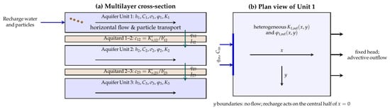
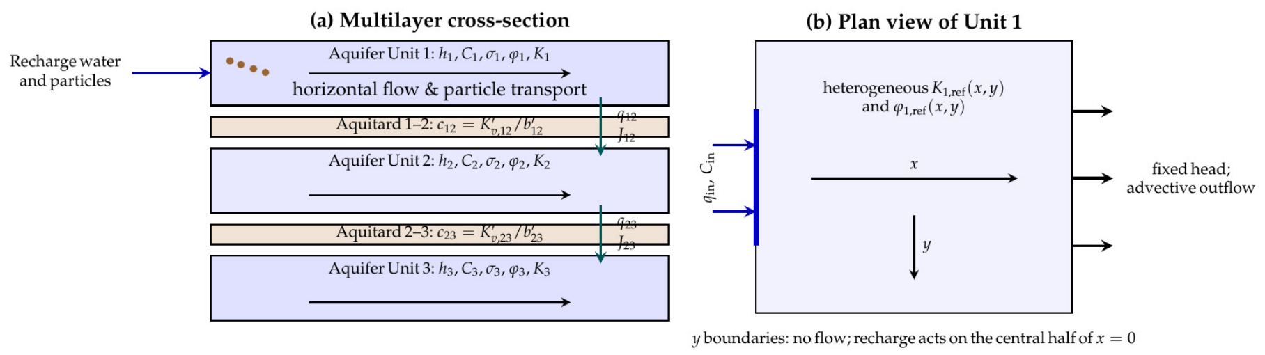
Figure 1 summarizes the quasi-three-dimensional representation, the horizontal boundary conditions, and the water and particle exchanges included in the model.

Figure 1. Conceptual model: (a) three laterally conductive aquifer units are coupled by stationary vertical water leakage and conservative advective particle exchange through two unresolved aquitards. Retained particles reduce porosity, matrix conductivity, and interface leakance. (b) In Unit 1, water and particles enter through the central half of the left boundary; prescribed heads and advective particle outflow are applied at the right boundary, and the lateral y boundaries are impermeable.

2.2. Horizontal Groundwater Flow

The layer-averaged flow equation is

$$S_k{\displaystyle \frac{\partial h_k}{\partial t}}={\nabla }_H·\left(T_k{\nabla }_H{h}_k\right)+R_k,T_k=b_k{K}_k$$

(1)

where S_k is the storage coefficient defined in Section 2.1, T_k is transmissivity (m² day⁻¹), K_k is horizontal hydraulic conductivity (m day⁻¹), and R_k is net vertical exchange (m day⁻¹). The horizontal Darcy flux is q_k = −K_k∇_Hh_k.

The reference conductivity relation distinguishes bulk porosity change from additional impairment associated with retained mass:

$$K_k=K_{k,\mathrm{r}\mathrm{e}\mathrm{f}}(x,y){\left(\frac{{\phi }_k}{{\phi }_{k,\mathrm{r}\mathrm{e}\mathrm{f}}}\right)}^{m_k}\mathrm{e}\mathrm{x}\mathrm{p}\left(-{\alpha }_k{\sigma }_k\right)$$

(2)

where m_k is dimensionless, and α_k has units m³ kg⁻¹. The clean reference fields are K_k,ref(x, y) = K_k,0F_k(x, y) and φ_k,ref(x, y) from Equation (11), where K_k,0 and φ_k,0 are the spatially uniform background values listed in Table 1 and F_k(x, y) is the dimensionless facies multiplier defined in Section 2.5 (F_k = 1 outside the lenses and the channel in Layers 1 and 2). Thus, the subscript “0” denotes a background constant, whereas “ref” denotes the spatially variable clean state before particle injection. The power term represents loss of bulk conducting volume, whereas the exponential term is an empirical proxy for stronger pore-throat or connected-porosity impairment. Its physical basis is the assumption that each increment of retained mass removes a constant fraction of the remaining hydraulic conductance, d(ln K_k)/dσ_k = −α_k. Such first-order damage behavior is expected when deposits accumulate preferentially in pore throats, which control hydraulic conductance far more strongly than pore bodies, so that conductivity declines faster than bulk porosity. For small α_kσ_k, the exponential factor coincides to first order with the hyperbolic formation-damage relation K/K₀ = (1 + β_dσ)⁻¹ used to describe injectivity decline caused by particle retention [21]. The exponential form nevertheless remains empirical: α_k is a lumped coefficient that is not derived from a resolved pore geometry and must be calibrated from column permeability and retained-mass data. Because that separation is not unique, two alternatives are tested: a porosity-only power law and the normalized Kozeny–Carman form

$${\displaystyle \frac{K_k}{K_{k,\mathrm{r}\mathrm{e}\mathrm{f}}}}={\left(\frac{{\phi }_k}{{\phi }_{k,\mathrm{r}\mathrm{e}\mathrm{f}}}\right)}^3{\left(\frac{1-{\phi }_{k,\mathrm{r}\mathrm{e}\mathrm{f}}}{1-{\phi }_k}\right)}^2$$

(3)

Equation (3) is the Kozeny–Carman relation normalized by the clean state, so that specific surface and tortuosity cancel under the assumption that deposition does not change them [22]. The relation was developed for granular media, and its predictive accuracy is lower for clay-bearing, poorly sorted, or structurally altered media [23]; for this reason, it is used here only as a sensitivity alternative rather than as a universally valid closure.

2.3. Particle Transport, Retention, and Porosity

The layer-integrated mobile-particle balance is

$$b_k{\displaystyle \frac{\partial \left({\phi }_k{C}_k\right)}{\partial t}}+{\nabla }_H·\left(b_k{\mathit{q}}_k{C}_k-b_k{\phi }_k{\mathit{D}}_k{\nabla }_H{C}_k\right)=b_k\left(-{\lambda }_k{C}_k+{\gamma }_k{\sigma }_k\left|{\mathit{q}}_k\right|\right)+J_k$$

(4)

where D_k is the horizontal dispersion tensor (m² day⁻¹), λ_k is the effective deposition rate (day⁻¹), γ_k is the effective re-entrainment coefficient (m⁻¹), and J_k is the net interlayer particle source (kg m⁻² day⁻¹). Retained mass and porosity evolve as

$${\displaystyle \frac{\partial {\sigma }_k}{\partial t}}={\lambda }_k{C}_k-{\gamma }_k{\sigma }_k\left|{\mathit{q}}_k\right|,{\phi }_k=\mathrm{m}\mathrm{a}\mathrm{x}\left({\varphi }_{\mathrm{r}\mathrm{e}\mathrm{s}},{\phi }_{k,\mathrm{r}\mathrm{e}\mathrm{f}}-{\beta }_k{\sigma }_k\right)$$

(5)

where β_k has units of m³ kg⁻¹. A general porosity dependence is available in the implementation,

$${\lambda }_k\left({\varphi }_k\right)={\lambda }_{k,0}{\left({\displaystyle \frac{{\varphi }_{k,\mathrm{r}\mathrm{e}\mathrm{f}}}{{\varphi }_k}}\right)}^{p_{\lambda ,k}},{\gamma }_k\left({\varphi }_k\right)={\gamma }_{k,0}{\left({\displaystyle \frac{{\varphi }_k}{{\varphi }_{k,\mathrm{r}\mathrm{e}\mathrm{f}}}}\right)}^{p_{\gamma ,k}}$$

(6)

The baseline uses p_λ,k = p_γ,k = 0 because no experiment is available to calibrate these exponents. Hence λ_k and γ_k must be interpreted as scenario-level effective coefficients, not universal material constants.

Equation (4) is a mass-conservation equation for suspended discrete particles represented at the continuum scale; it is not a dissolved-solute transport equation. The advective term transports particle mass with the Darcy flux, while D_k represents effective hydrodynamic and mechanical spreading of the suspended phase rather than molecular Fickian diffusion. Deposition and re-entrainment are represented separately through the exchange terms in Equations (5) and (6), consistent with continuum filtration descriptions and contemporary pore-scale evidence [8,9,11,12].

Equations (4)–(6) do not account explicitly for particle size. Size-dependent mechanisms, such as size exclusion, straining at pore throats smaller than a critical particle-to-grain diameter ratio, gravitational settling, and bridging, are not represented by separate terms. Their aggregate effect is absorbed into the effective coefficients λ_k, γ_k, D_k, β_k, and α_k, which therefore apply only to the representative 10 µm particle class and the specified inlet concentration. A different particle-size distribution would require recalibration of these coefficients or a size-resolved, multi-class formulation.

2.4. Aquitard Leakage and Interlayer Particle Exchange

Clean aquitard leakance is calculated from its vertical conductivity K′_v,p and thickness b′_p:

$$c_{p,\mathrm{r}\mathrm{e}\mathrm{f}}(x,y)={\zeta }_p(x,y){\displaystyle \frac{K_{v,p}^{\text{'}}}{b_p^{\text{'}}}},p\in \left\{12|,|23\right\}$$

(7)

where c has units of day^−1, and ζ_p is a prescribed dimensionless heterogeneity multiplier. Physically, ζ_p(x, y) represents lateral variation in the effective vertical conductivity or thickness of the clean aquitard, for example, finer-grained or thicker aquitard material beneath fine-grained facies of the adjacent aquifers. It is a property of the clean aquitard and is independent of particle retention: ζ_p modifies c_p,ref before clogging, whereas the clogging effect enters only through η_p in Equation (8). In the reference case, ζ_p = 1 except over the lens unions described in Section 2.5, where ζ₁₂ = 0.40 and ζ₂₃ = 0.55. The resulting reductions (factors of 2.5 and 1.8) are synthetic and are smaller than the aquifer-lens conductivity contrasts, so the leakance field is heterogeneous without dominating the lateral flow pattern. In the homogeneous experiment, ζ_p = 1 everywhere, giving c_12,0 = 0.0025 day⁻¹ and c_23,0 = 0.0008 day⁻¹ (Table 1). Clogging-sensitive leakage is

$$q_{12}=c_{12}\left(h_1-h_2\right),c_{12}=c_{12,\mathrm{r}\mathrm{e}\mathrm{f}}\mathrm{e}\mathrm{x}\mathrm{p}\left[-{\displaystyle \frac{{\eta }_{12}}{2}}\left({\sigma }_1+{\sigma }_2\right)\right],$$

$$q_{23}=c_{23}\left(h_2-h_3\right),c_{23}=c_{23,\mathrm{r}\mathrm{e}\mathrm{f}}\mathrm{e}\mathrm{x}\mathrm{p}\left[-{\displaystyle \frac{{\eta }_{23}}{2}}\left({\sigma }_2+{\sigma }_3\right)\right]$$

(8)

with η_p in m³ kg⁻¹. Because the aquitards are unresolved interfaces, particles retained within them are not tracked, and interface impairment must be expressed through the retained contents of the adjacent units. The reference closure places the arithmetic mean of σ in the exponent, which is equivalent to the geometric mean of the two one-sided impairment factors exp(−η_pσ) of the upper and lower units. It represents an interface whose effective conductance is reduced with equal weight by fine deposits in both contact zones, i.e., the base of the upper unit and the top of the lower unit, and it is symmetric with respect to the flow direction. This assumption is a closure choice rather than a relation derived from a published interface-clogging law. Three alternative closures were therefore examined. Writing c₁₂ = c_12,refΦ₁₂ (and analogously for interface 2–3), the alternatives are

$${\Phi }_{12}^D=\mathrm{e}\mathrm{x}\mathrm{p}\left(-{\eta }_{12}{\sigma }_{12}^{\mathrm{u}\mathrm{p}}\right),{\Phi }_{12}^S={\displaystyle \frac{2}{e^{{\eta }_{12}{\sigma }_1}+e^{{\eta }_{12}{\sigma }_2}}},{\Phi }_{12}^M=\mathrm{e}\mathrm{x}\mathrm{p}\left[-{\eta }_{12}\mathrm{m}\mathrm{a}\mathrm{x}\left({\sigma }_1,{\sigma }_2\right)\right]$$

(9)

where σ^up₁₂ is the retained content of the donor unit selected by the sign of q₁₂, as for the particle flux in Equation (10). The donor closure Φ^D assumes that sealing occurs mainly on the inflow face of the aquitard, analogous to an external filter cake. The series closure Φ^S treats the aquitard as two halves of equal clean resistance, each impaired by the adjacent unit, and adds their hydraulic resistances. The maximum closure Φ^M is a conservative upper-bound choice. To first order in η_pσ, the reference and series closures are identical, ln Φ ≈ −η_p(σ₁ + σ₂)/2, whereas, for downward flow, the donor closure gives ln Φ ≈ −η_pσ₁ at interface 1–2 and −η_pσ₂ at interface 2–3, which is approximately twice the reference value when retention in the upper unit dominates. The closure therefore matters mainly where retention is strongly asymmetric across an interface, as it is near the recharge boundary.

The source terms in Equation (1) are R₁ = −q₁₂, R₂ = q₁₂ − q₂₃, and R₃ = q₂₃, so their sum is zero pointwise.

Interlayer particle transfer is advective in the baseline:

$$J_{12}=q_{12}{C}_{12}^{\mathrm{u}\mathrm{p}},J_{23}=q_{23}{C}_{23}^{\mathrm{u}\mathrm{p}}$$

(10)

where the donor concentration is selected according to the sign of the water flux. The corresponding layer sources are J₁ = −J₁₂, J₂ = J₁₂ − J₂₃, and J₃ = J₂₃; therefore, interlayer particle transfer is conservative.

2.5. Two-Dimensional Heterogeneity, Initial State, and Boundaries

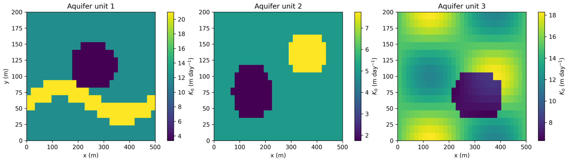
The reference fields are deterministic so that every result can be reproduced. Layer 1 contains an elliptical low-conductivity lens with multiplier 0.28 and a sinuous high-conductivity channel with multiplier 1.75. Layer 2 contains low- and high-conductivity lenses with multipliers 0.35 and 1.55. Layer 3 combines a smooth multiplier with a low-conductivity lens multiplier of 0.45. The smooth multiplier is

$$1+0.22\mathrm{s}\mathrm{i}\mathrm{n}\left({\displaystyle \frac{2\pi x}{L_x}}\right)\mathrm{c}\mathrm{o}\mathrm{s}\left({\displaystyle \frac{2\pi y}{L_y}}\right)$$

The lenses are elliptical inclusions with abrupt boundaries, within which the background conductivity is multiplied by the stated factor (Section 3.2). In Layer 1, the low-conductivity lens is centered at (0.52L_x, 0.58L_y) = (260, 116) m with semi-axes 0.18L_x = 90 m and 0.19L_y = 38 m. The high-conductivity channel is a band of half-width 0.07L_y = 14 m around the sinuous centerline y = 0.30L_y + 0.10L_y sin(2πx/L_x), extending across the full domain length; its multiplier is assigned after that of the lens and therefore takes precedence where the two overlap. In Layer 2, the low-conductivity lens is centered at (150, 76) m with semi-axes of 80 m and 44 m, and the high-conductivity lens at (360, 136) m with semi-axes of 75 m and 34 m. In Layer 3, the low-conductivity lens is centered at (310, 70) m with semi-axes of 100 m and 40 m, and its multiplier 0.45 is applied to the smooth background multiplier given above. The lenses therefore occupy different positions in the three units.

In the smooth multiplier, which applies to Layer 3, the amplitude 0.22 gives a ±22% background modulation of conductivity. This variability is deliberately weaker than the discrete lens contrasts (multipliers 0.28–1.75), so the facies structure remains identifiable. A single wavelength in each direction places the modulation at the domain scale, where it is resolved by many cells on all grids used. Reference porosity varies as

$${\varphi }_{k,\mathrm{r}\mathrm{e}\mathrm{f}}(x,y)=\mathrm{c}\mathrm{l}\mathrm{i}\mathrm{p}\left({\varphi }_{k,0}\left[1+0.045\mathrm{s}\mathrm{i}\mathrm{n}(2\pi x/L_x)\mathrm{c}\mathrm{o}\mathrm{s}(2\pi y/L_y)\right],{\varphi }_{k,0}-0.035,{\varphi }_{k,0}+0.035\right)$$

(11)

The relative amplitude 0.045 produces absolute porosity variations of at most 0.045φ_k,0, i.e., 0.014–0.017 for the three units, so heterogeneity enters mainly through K_k,ref rather than through φ_k,ref. The clipping bounds φ_k,0 ± 0.035 are a safeguard that keeps reference porosity within a physically plausible band if the amplitude is increased in sensitivity runs; for the reference amplitude, they are never active. All of these coefficients are synthetic design values, not site estimates. The c₁₂ field is multiplied by 0.40 over the union of the Layer 1 and Layer 2 low-conductivity lenses; c₂₃ is multiplied by 0.55 over the union of the Layer 2 high-conductivity lens and Layer 3 low-conductivity lens, i.e., ζ₁₂ = 0.40 and ζ₂₃ = 0.55 there and ζ_p = 1 elsewhere. Exact lens equations and ordering are supplied in Supplementary Code S2.

At x = 0, a Darcy recharge flux of 0.060 m day⁻¹ enters Layer 1 only over 0.25L_y ≤ y ≤ 0.75L_y; the remaining part of that boundary is impermeable. The injected concentration is 0.050 kg m⁻³ (50 mg L⁻¹). Fixed heads of 45, 44, and 43 m are imposed at x = L_x in Layers 1–3, respectively. The y boundaries are no-flow boundaries, and particles leave advectively at the right boundary. Initially, C_k = σ_k = 0 and φ_k = φ_k,ref. Rather than prescribing an arbitrary head profile, h_k(x, y, 0) is obtained by solving the clean, steady, coupled flow problem under the same hydraulic boundaries. This construction removes initial hydraulic relaxation from the subsequent clogging comparison.

2.6. Spatial and Temporal Discretization

The domain is divided into N_x × N_y cell-centered finite volumes with Δx = L_x/N_x and Δy = L_y/N_y. At an internal face, transmissivity is the harmonic mean

$$T_{i+1/2,j,k}={\displaystyle \frac{2T_{i,j,k}{T}_{i+1,j,k}}{T_{i,j,k}+T_{i+1,j,k}}}$$

(12)

which gives the correct series resistance across an abrupt conductivity jump. For example, the conservative second-order x operator is

$${\mathcal{L}}_x{h}_{i,j,k}={\displaystyle \frac{1}{\Delta x^2}}\left[T_{i+1/2,j,k}\left(h_{i+1,j,k}-h_{i,j,k}\right)-T_{i-1/2,j,k}\left(h_{i,j,k}-h_{i-1,j,k}\right)\right]$$

(13)

with an analogous expression in y.

The flow step uses a Peaceman–Rachford alternating-direction implicit (ADI) scheme [24,25]. Each directional sweep gives independent tridiagonal systems. Conductivity and aquitard source terms are updated by Picard iteration. Convergence is declared when

$${\mathrm{m}\mathrm{a}\mathrm{x}}_k\Vert h_k^{r+1}-h_k^r{\Vert }_{\mathrm{\infty }}\le {\epsilon }_{\mathrm{a}\mathrm{b}\mathrm{s}}+{\epsilon }_{\mathrm{r}\mathrm{e}\mathrm{l}}\mathrm{m}\mathrm{a}\mathrm{x}\left(h_s,{\mathrm{m}\mathrm{a}\mathrm{x}}_k[{\mathrm{m}\mathrm{a}\mathrm{x}}_{\Omega }{h}_k^{r+1}-{\mathrm{m}\mathrm{i}\mathrm{n}}_{\Omega }{h}_k^{r+1}]\right)$$

(14)

where ε_abs = 10⁻⁹ m, ε_rel = 10⁻⁸, and the dimensional reference scale is h_s = 1 m. The criterion uses only head differences and iterative updates and is therefore invariant to the selected vertical datum. The maximum (L∞) norm is used rather than a discrete L2 norm because the nonlinearity is concentrated in a small region near the recharge strip and the clogging front, where conductivity and leakance change most rapidly. A global L2 norm averages the update over all cells; unless it is normalized, its value depends on the number of cells, and a large but localized non-converged update can be diluted by the many cells that have already converged. The L∞ criterion instead requires every cell in every layer to satisfy the tolerance, so local errors near the clogging front cannot be hidden, and the criterion has the same meaning on all grids of the refinement study. Under-relaxation is applied only within the Picard loop. Iterative nonlinear groundwater methods are discussed by Mehl [26].

Mobile-particle advection is discretized by first-order upwinding, and dispersion uses centered face gradients. The explicit transport step is automatically divided into substeps so that a combined advection–dispersion–interlayer Courant number does not exceed 0.75. For the local reaction, let m_k = φ_kC_k, M_k = m^∗_k + σⁿ_k, κ^dep_k = λ_k/φ_k, and κ^re_k = γ_k|q_k|. The semi-implicit update is

$$m_k^{n+1}={\displaystyle \frac{m_k^{\ast }+\Delta t{\kappa }_k^{\mathrm{r}\mathrm{e}}{M}_k}{1+\Delta t\left({\kappa }_k^{\mathrm{d}\mathrm{e}\mathrm{p}}+{\kappa }_k^{\mathrm{r}\mathrm{e}}\right)}},{\sigma }_k^{n+1}=M_k-m_k^{n+1}$$

(15)

This step is positivity preserving for nonnegative states and conserves local mobile-plus-retained-particle content algebraically. The complete sequentially coupled algorithm is first-order in time; its upwind advective component is first-order in space, whereas the horizontal diffusion operator is second-order. Consequently, the second-order spatial accuracy demonstrated for the ADI flow solver in Section 3.1 is a property of that component only and is not expected for the coupled model.

2.7. Reference Parameters and Experimental Design

The domain and numerical settings are listed in Table 1, and the aquifer-specific hydraulic and effective particle-retention parameters are summarized in Table 2. The aquitard vertical conductivities, 0.0050 and 0.0024 m day⁻¹, are three to four orders of magnitude lower than the aquifer-unit conductivities. They also lie within the broad range reported for clay- and silt-rich aquitards, but remain synthetic rather than site-calibrated [27]. The 10 µm particle lies within the 3–30 µm interval used in a recent suspended-fines experiment; the present 50 mg L⁻¹ inlet concentration is lower than that study’s 100–400 mg L⁻¹ range [28].

Table 2. Aquifer-unit and effective particle-retention parameters.

Parameter	Unit 1	Unit 2	Unit 3	Units
Background conductivity Kk,0	12	5	15	m day−1
Background porosity φk,0	0.35	0.32	0.38	–
Storage coefficient Sk	0.12	0.08	0.15	–
Porosity exponent m	3	3	3	–
Retained-mass sensitivity α	9	12	6	m3 kg−1
Porosity-loss coefficient β	1.20	0.90	0.70	m3 kg−1
Deposition rate λ0	0.060	0.035	0.020	day−1
Re-entrainment coefficient γ0	0.006	0.005	0.004	m−1
Dispersion coefficient D	0.60	0.35	0.70	m2 day−1

Background values K_k,0 and φ_k,0 are combined with the facies multipliers F_k(x, y) and Equation (11) to give the clean reference fields K_k,ref(x, y) and φ_k,ref(x, y) used in Equations (2) and (3).

Table 2. Aquifer-unit and effective particle-retention parameters.

Parameter	Unit 1	Unit 2	Unit 3	Units
Background conductivity Kk,0	12	5	15	m day−1
Background porosity φk,0	0.35	0.32	0.38	–
Storage coefficient Sk	0.12	0.08	0.15	–
Porosity exponent m	3	3	3	–
Retained-mass sensitivity α	9	12	6	m3 kg−1
Porosity-loss coefficient β	1.20	0.90	0.70	m3 kg−1
Deposition rate λ0	0.060	0.035	0.020	day−1
Re-entrainment coefficient γ0	0.006	0.005	0.004	m−1
Dispersion coefficient D	0.60	0.35	0.70	m2 day−1

Background values K_k,0 and φ_k,0 are combined with the facies multipliers F_k(x, y) and Equation (11) to give the clean reference fields K_k,ref(x, y) and φ_k,ref(x, y) used in Equations (2) and (3).

Four matched experiments are evaluated. In the full-clogging case, matrix and interface feedbacks are active. In the clean-interface case, particle and matrix clogging remain active, but η₁₂ = η₂₃ = 0. In the hydraulic control, no particles are injected, and all clogging feedbacks are disabled. In the homogeneous full-clogging case, the spatial facies and leakance multipliers are removed while the mean-scale parameters and clogging processes remain active. This factorial structure separates initial hydraulic response, matrix impairment, interface sealing, and spatial heterogeneity.

2.8. Verification and Sensitivity Tests

The ADI head solver is tested against

$$h_{\mathrm{e}\mathrm{x}}=\mathrm{s}\mathrm{i}\mathrm{n}\left({\displaystyle \frac{\pi x}{L}}\right)\mathrm{s}\mathrm{i}\mathrm{n}\left({\displaystyle \frac{\pi y}{L}}\right)\mathrm{e}\mathrm{x}\mathrm{p}\left(-{\displaystyle \frac{2{\pi }^{2}at}{L^2}}\right)$$

(16)

the exact solution of h_t = a(h_xx + h_yy) with homogeneous Dirichlet boundaries. Separate analytical tests examine the local deposition–re-entrainment update and periodic one-dimensional advection–dispersion. Additional tests verify pointwise interlayer conservation, global particle mass balance, positivity, and invariance to a 100 m shift in the hydraulic datum. Coupled grid/time calculations use 21 × 11 cells with Δt = 1 day, 31 × 17 with 0.5 day, 41 × 23 with 0.25 day, and 61 × 35 with 0.125 day. Finally, the reference conductivity law is compared with the porosity-only and Kozeny–Carman alternatives; the reference interface closure is compared with the donor, series, and maximum closures of Equation (9) relative to a common clean-interface control, and the reference storage coefficients are compared with S_k = 0.01 in all units, and low/reference/high clogging-parameter sets are examined.

Verification is therefore performed at two distinct levels. At the component level, Equation (16) and the separate reaction and transport benchmarks verify individual operators against analytical solutions. At the system level, no analytical solution exists for the fully coupled flow–transport–retention–leakage problem; the coupled model is verified only through conservation identities, positivity, datum invariance, and grid/time refinement. These system-level tests demonstrate consistency and convergence of the coupled results, but they do not establish a formal order of accuracy for the coupled model.

3. Results

3.1. Numerical Verification

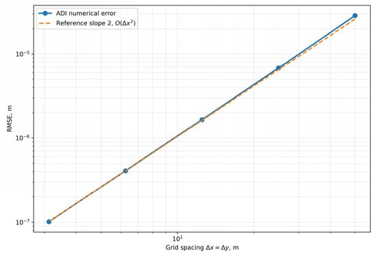
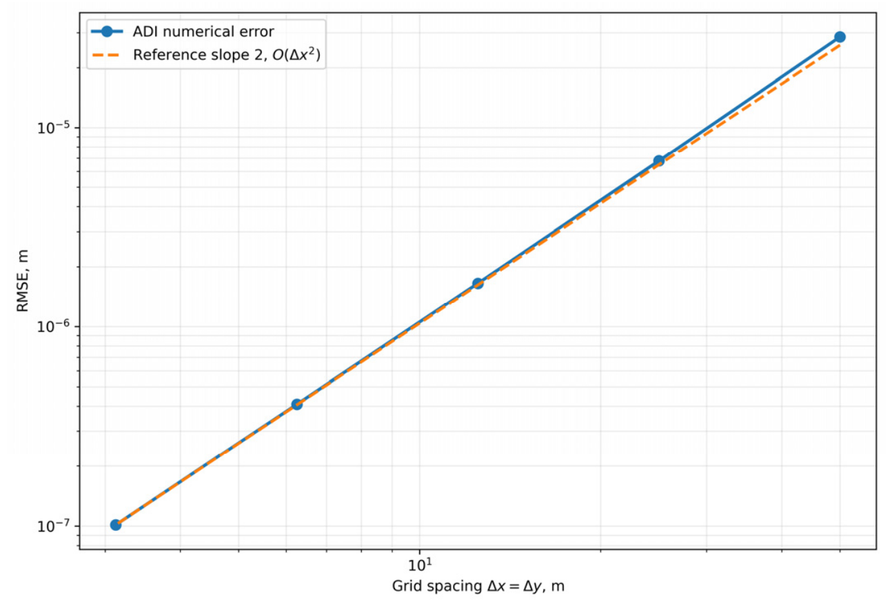
The manufactured-solution test approaches second-order spatial convergence, with an observed order of 2.009 on the finest grid (Table 3 and Figure 2); this order characterizes the ADI flow solver alone. The semi-implicit reaction benchmark approaches first-order temporal convergence, with order 0.992 at the smallest tested step. The periodic transport benchmark approaches first-order convergence, with order 0.997 on the finest grid, as expected from upwind advection. A 100 m datum shift changes every computed head by 100 m but leaves head differences, leakage, and the stopping tolerance unchanged. The maximum relative global particle mass-balance residual among the reported coupled runs is 1.53 × 10⁻¹⁴.

Table 3. Spatial convergence of the ADI head solver.

Points Per Direction	Δx = Δy, m	RMSE, m	Observed Order
11	50.000	2.859 × 10−5	–
21	25.000	6.787 × 10−6	2.074
41	12.500	1.654 × 10−6	2.037
81	6.250	4.084 × 10−7	2.018
161	3.125	1.015 × 10−7	2.009

Figure 2. Grid-refinement error for the two-dimensional manufactured solution.

These results must be interpreted at two levels. The flow solver has been verified against an exact analytical solution and is second-order accurate in space; the reaction and transport substeps have each been verified against their own analytical solutions and are first-order accurate. The fully coupled model has no analytical benchmark, and its sequential coupling and upwind advection make it formally first-order. Its verification therefore rests on the conservation, positivity, and invariance tests above and on the grid/time refinement in Section 3.5. The second-order convergence of the flow solver is not claimed for the coupled model.

3.2. Realization of Two-Dimensional Heterogeneity

Figure 3 shows that each aquifer unit contains a distinct conductivity architecture rather than a layerwise constant value. The nonuniform recharge strip intersects only part of the Layer 1 boundary, generating both x- and y-directed head and concentration gradients. The heterogeneous full-clogging run gives final mean leakage values 4.24% lower at interface 1–2 and 8.77% lower at interface 2–3 than the homogeneous full-clogging run. Thus, the absolute interlayer exchange is sensitive to the spatial facies and aquitard-leakance arrangement even though the particle-induced percentage changes remain small.

Figure 3. Reference horizontal conductivity fields in the three aquifer units. The recharge strip occupies the central half of the left boundary in Unit 1.

Figure 3. Reference horizontal conductivity fields in the three aquifer units. The recharge strip occupies the central half of the left boundary in Unit 1.

3.3. Clogging Pattern and Matrix-Conductivity Change

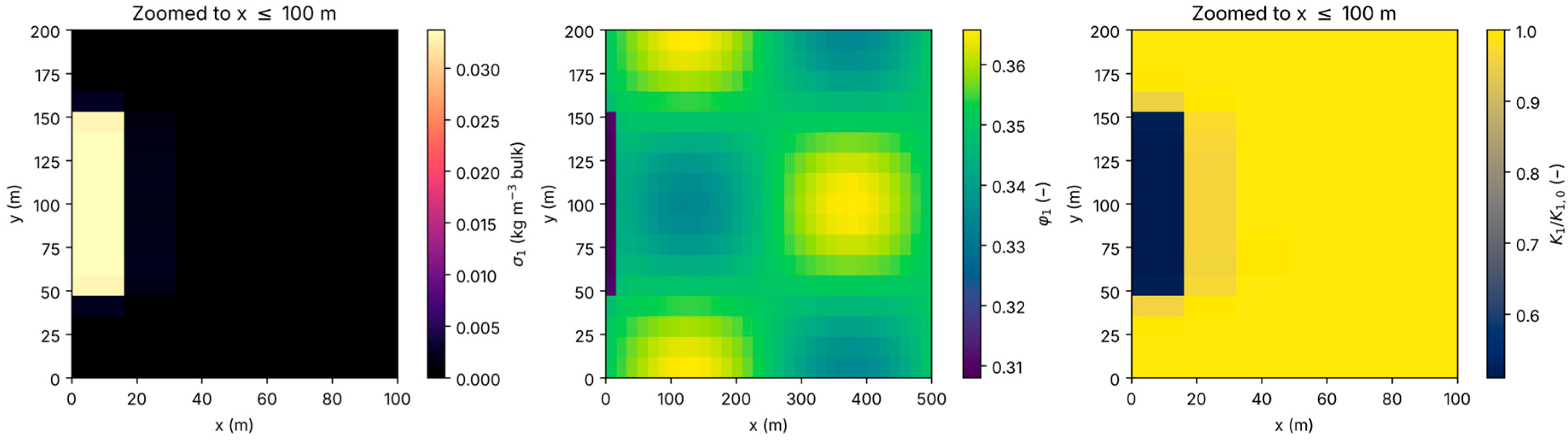
Retained particles remain concentrated near the active recharge segment (Figure 4). This spatial localization follows from the imposed particle source, first-order deposition, and progressive reduction in local conductivity. After 200 days, the spatially averaged conductivity of Unit 1 decreases by 1.038%. Changes in Units 2 and 3 are much smaller because most mobile mass is retained before reaching the deeper units. The porosity field changes modestly, whereas K₁/K_1,ref shows a stronger localized response, illustrating why total porosity loss and connected-flow impairment should not be treated as identical observables.

Figure 4. Full-clogging result in aquifer Unit 1 after 200 days: retained-particle content, porosity, and normalized hydraulic conductivity. The retained-particle and conductivity panels are cropped to x ≤ 100 m because both effects are confined to the recharge-affected zone (x ≲ 56 m); the porosity panel retains the full 500 m domain because its background heterogeneity extends across it.

3.4. Causal Separation of Leakage Responses

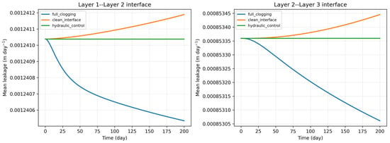
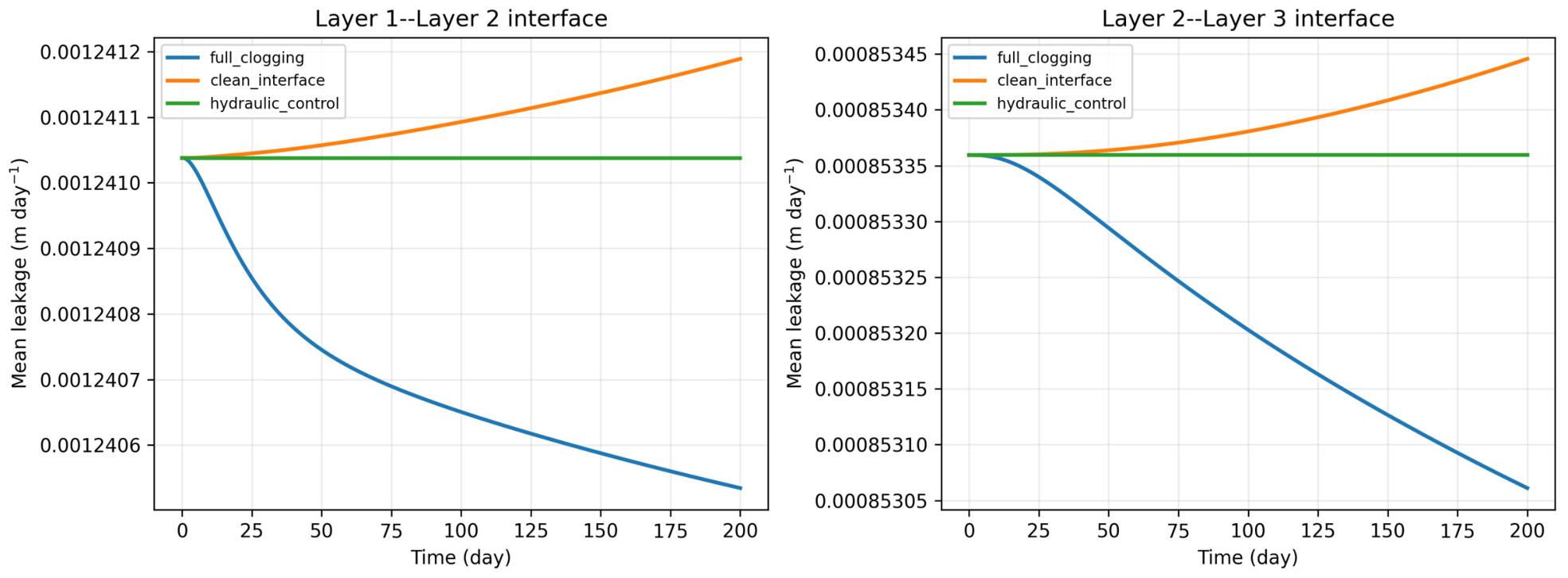
The leakage trajectories are compared in Figure 5, and their endpoint metrics are reported in Table 4. The no-particle hydraulic control remains stationary to numerical precision because the clean steady hydraulic solution is used as the initial state. In the full-clogging case, q₁₂ changes from 0.00124104 to 0.00124053 m day⁻¹, a decrease of 0.0406%; q₂₃ decreases by 0.0350%. The clean-interface case exhibits small increases of 0.0122% and 0.0101% because matrix impairment slightly redistributes the horizontal head field while interface conductance is held fixed. Comparing the full-clogging and clean-interface endpoints directly isolates the interface feedback: it changes q₁₂ by −0.0528% and q₂₃ by −0.0451%. This interface effect exceeds the differences among the three finest grid/time levels of the full-clogging response (at most 0.0033 and 0.0028 percentage points for q₁₂ and q₂₃; Table 5) by more than an order of magnitude, so it is numerically resolved. Its physical significance is discussed in Section 4.2.

Figure 5. Mean leakage at the two aquitards for the full-clogging, clean-interface, and no-particle hydraulic-control experiments.

Table 4. Endpoint metrics for the causal controls and homogeneous comparison.

Case	q12(0), m day−1	q12(200), m day−1	Δq12, %	Δq23, %	$\mathbf{\Delta }{\overline{\mathit{K}}}_{\mathbf{1}}$, %
Full clogging	0.00124104	0.00124053	−0.0406	−0.0350	−1.038
Clean interface	0.00124104	0.00124119	+0.0122	+0.0101	−1.038
Hydraulic control	0.00124104	0.00124104	<10−9	<10−9	0
Homogeneous full	0.00129588	0.00129542	−0.0350	−0.0291	−0.915

Table 5. Coupled grid/time sensitivity after 200 days.

Case	Grid	Δt, Day	Δq12, %	Δq23, %
Coarse	21 × 11	1.000	−0.0306	−0.0261
Reference	31 × 17	0.500	−0.0406	−0.0350
Fine	41 × 23	0.250	−0.0373	−0.0322
Very fine	61 × 35	0.125	−0.0393	−0.0341

3.5. Grid/Time and Constitutive Sensitivity

The normalized leakage changes approach stable values as both grid and time step are refined (Table 5). The reference and very-fine values differ by 0.0013 percentage points for q₁₂ and 0.0009 percentage points for q₂₃. The mean Unit 1 conductivity loss is less regular because the affected region is narrow and its cell-average representation changes as the boundary cells and facies masks are refined. This limitation is reported explicitly rather than hidden by quoting more significant digits.

The conductivity closure changes the mean Unit 1 reduction from 0.570% for the porosity-only law to 0.733% for Kozeny–Carman and 0.954% for the combined power and exponential law on the common coarse sensitivity grid. Low, reference, and high clogging-parameter sets give Unit 1 conductivity reductions of 0.310%, 0.954%, and 2.422%, respectively. Over the same range, q₁₂ changes from −0.0075% to −0.2290%, and q₂₃ from −0.0063% to −0.1531%. Table 6 summarizes these constitutive and parameter-range results. The response direction is robust, but its magnitude depends on effective retention and conductivity parameters.

Table 6. Constitutive-law and clogging-range sensitivity on the common 21 × 11, 1-day grid.

Case	$\mathbf{\Delta }{\overline{\mathit{K}}}_{\mathbf{1}}$, %	Δq12, %	Δq23, %
Power plus exponential	−0.954	−0.0306	−0.0261
Porosity-only power	−0.570	−0.0361	−0.0308
Kozeny–Carman	−0.733	−0.0340	−0.0290
Low clogging range	−0.310	−0.0075	−0.0063
Reference clogging range	−0.954	−0.0306	−0.0261
High clogging range	−2.422	−0.2290	−0.1531

Table 7 compares the interface closures of Equation (9). For each closure, the interface effect is the difference between the full-clogging change and the change in the common clean-interface control on the 21 × 11, 1-day grid. The series closure changes the interface effect by less than 0.002 percentage points relative to the reference closure (−0.0450 versus −0.0432 for q₁₂ and −0.0379 versus −0.0367 for q₂₃), consistent with their first-order equivalence. The donor and maximum closures give identical results because retention decreases downward, so the donor unit is also the more strongly clogged unit at both interfaces; they approximately double the interface effect, to −0.0833 and −0.0715 percentage points. The closure therefore changes the magnitude of the interface contribution by up to a factor of about two but not its sign, and in all cases the effect remains below 0.1%. The mean Unit 1 conductivity loss is identical for all closures (−0.954%).

Table 7. Sensitivity of leakage to the interface-clogging closure and storage coefficient on the common 21 × 11, 1-day grid. The interface effect is the full-clogging change minus the clean-interface change, in percentage points (pp).

Case	Δq12, %	Δq23, %	Interface Effect on q12, pp	Interface Effect on q23, pp
Clean interface (ηp = 0)	+0.0127	+0.0107	0	0
Arithmetic mean, Equation (8) (reference)	−0.0306	−0.0261	−0.0432	−0.0367
Donor unit only, ΦD	−0.0707	−0.0608	−0.0833	−0.0715
Series resistance, ΦS	−0.0324	−0.0272	−0.0450	−0.0379
Maximum, ΦM	−0.0707	−0.0608	−0.0833	−0.0715
Reference closure, Sk = 0.01	−0.0138	−0.0185	−0.0275	−0.0371

The last row of Table 7 repeats the reference closure with S_k = 0.01 in all units, which shortens the diffusive response times to about 17, 63, and nine days, with its own clean-interface control. The interface effect at interface 2–3 is practically unchanged (−0.0371 versus −0.0367 percentage points), whereas that at interface 1–2 decreases by about one-third (−0.0275 versus −0.0432 percentage points). Part of the 200-day response at the upper interface therefore reflects storage lag, but the sign and order of magnitude of the interface effect are unchanged.

3.6. Global Particle Mass Balance

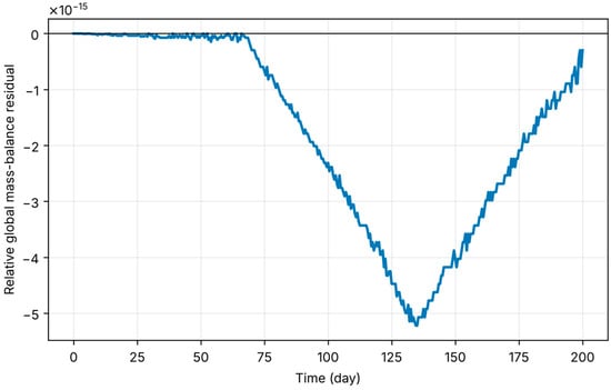
The global particle inventory equals cumulative particle inflow minus outflow to round-off (Figure 6). The reference run’s maximum relative residual is 5.22 × 10⁻¹⁵, and the very-fine run’s value is 1.53 × 10⁻¹⁴. This check includes lateral transport, interlayer advection, and mobile-to-retained transfer; it therefore tests the coupled particle subsystem rather than the head solver alone.

Figure 6. Relative global particle mass-balance residual for the reference full-clogging experiment.

4. Discussion

4.1. Mechanistic Interpretation and Relation to Published Work

The simulated clogging front develops near the particle-bearing boundary, which is consistent with MAR studies that report near-surface or near-inlet accumulation of intrusive fines [16,17,18]. Resolved CFD–DEM and pore-network studies show that local bridging and jamming depend on constriction geometry and particle interactions [10,11,12,13]. The present continuum model does not resolve those mechanisms. Instead, their net effect is represented by λ, γ, β, and α. This scale distinction explains why a representative diameter is reported but does not appear directly in Equations (4)–(6).

The framework used to reduce conductivity is conceptually consistent with Glass et al. [14], who used scaling factors in HYDRUS to represent conductivity losses caused by clogging in recharge wells and infiltration basins. In contrast, the present formulation couples particle retention to both matrix-conductivity degradation and interlayer leakage within a laterally heterogeneous multilayer aquifer system.

The mean Unit 1 conductivity loss is modest compared with the severe decreases observed in some high-concentration laboratory systems [19]. That difference is physically plausible: the present inlet concentration is 50 mg L⁻¹, parameters are deliberately moderate, and the affected area occupies a small part of the full horizontal domain. The result should therefore be read as a synthetic process demonstration, not as a universal MAR clogging rate.

The main causal finding concerns leakage. Aquitard flow depends on both conductance and the evolving head difference. Matrix clogging can increase or decrease that head difference, while interface deposition reduces conductance. A raw time-series decline mixes these effects with initial hydraulic equilibration. By starting from the clean steady solution and comparing matched controls, the present experiment shows that interface clogging changes leakage by only approximately 0.05% under the reference parameters. Had the transient started from an arbitrarily prescribed non-equilibrium head field, the resulting leakage decline would have been dominated by hydraulic relaxation and could not have been attributed to clogging. This result reinforces the need for a no-clogging baseline in process attribution.

4.2. Physical Significance of the Small Interface Effect

The interface effect of about 0.05% must be interpreted as numerically significant but not physically significant. It is numerically significant because it exceeds the differences among the finest grid/time levels by more than an order of magnitude and the relative particle mass-balance residual by about ten orders of magnitude, and because the matched controls remove hydraulic relaxation from the comparison. It is not physically significant in the sense of being measurable or decision-relevant. Field estimates of aquitard leakage are derived from head differences and vertical conductivities whose uncertainty is expressed in factors rather than fractions of a percent, so a 0.05% change could not be detected. Moreover, the effective coefficients η_p, λ_k, and α_k are uncalibrated: the parameter-range tests alone change the full-clogging leakage response by a factor of about 30 (−0.0075% to −0.2290% for q₁₂; Table 6), and the interface closure changes the interface effect by up to a factor of about two (Table 7). The small reference value should therefore not be read as evidence that interface clogging is generally negligible in MAR systems.

The spatial mean also conceals a localized effect. Retained mass is confined to the recharge-affected zone (x ≲ 56 m), where σ₁ approaches 0.03 kg m⁻³ (Figure 4). With σ₂ ≈ 0 and η₁₂ = 6 m³ kg⁻¹, Equation (8) gives a local leakance reduction of about 1 − exp(−0.09) ≈ 9% in the most strongly clogged cells, but these cells occupy less than about 3% of the interface area, so the domain-averaged change is strongly diluted. Interface clogging could become physically relevant at higher influent concentrations, over longer operating periods, for larger η_p, for recharge distributed over a larger part of the domain, or when the quantity of interest is local exchange beneath an infiltration facility rather than domain-averaged leakage. The present result is therefore an attribution-focused demonstration: it shows how the interface contribution can be isolated, not how large it is at a real site. Establishing its physical magnitude requires column experiments with measured retained-mass profiles and vertical conductance across a fine-grained interface.

4.3. Constitutive Uncertainty

Equation (5) links deposited mass to total porosity, whereas hydraulic conductivity responds mainly to the continuity and size of connected-pore throats. A small change in bulk porosity can therefore accompany a larger conductivity reduction. The exponential factor in Equation (2) represents this additional impairment empirically; it is not derived from a resolved pore geometry. The sensitivity analysis shows that changing the closure alters the predicted Unit 1 conductivity loss by a factor of approximately 1.7. This spread shows that the conductivity–porosity law cannot be treated as innocuous. The interface closure in Equation (8) is a second structural assumption of the same kind; Table 7 quantifies its influence, and direct measurements of conductance across a clogged aquifer–aquitard contact would be needed to select among the closures.

The effective deposition and re-entrainment rates are likewise uncertain. Attachment, straining, bridging, and hydrodynamic release may respond differently to velocity, concentration, particle size, surface chemistry, and porosity [9,11,12]. Equation (6) permits porosity-dependent coefficients, but the baseline exponents are zero because no calibration dataset is available. Fitting these coefficients to column breakthrough curves and retained-mass profiles would be required before predictive use.

4.4. Applicability and Limitations

The model uses a quasi-three-dimensional geometry consistent with the leakage equations, realizes internal two-dimensional heterogeneity, applies harmonic face averaging, uses a datum-invariant nonlinear tolerance, begins from hydraulic equilibrium, and includes component-level and coupled conservation tests. These features make the numerical experiment reproducible and the attribution of small leakage effects defensible.

Numerical verification and physical validation have different roles in this study. The analytical benchmarks, conservation identities, datum-shift test, grid/time refinement, matched controls, and constitutive sensitivity tests establish numerical consistency and robustness for the stated equations, but they do not establish site-specific predictive accuracy. Because no suitable field or column dataset is available, the model is not presented as calibrated or physically validated. Its qualitative behavior—inlet-localized retention followed by conductivity reduction—is nevertheless consistent with published laboratory, imaging, and field-oriented MAR observations [16,17,18,19]. Here, reproducibility means that readers can repeat and audit the defined synthetic experiment; it does not imply that the resulting parameter set can be transferred directly to a field site.

Several limitations remain. No field or column dataset is used for calibration or physical validation. The facies fields are deterministic synthetic structures rather than geostatistical realizations. The model is saturated and isothermal; it omits unsaturated infiltration, geochemistry, biomass growth, particle-size distributions, and explicit pore-scale forces. Aquitard particle storage is represented only through adjacent-unit retained mass, because the aquitards are unresolved interfaces, and the weighting of the two sides is a closure assumption whose influence is examined in Table 7. The storage coefficients are effective specific-yield-type values; because the resulting diffusive response times are comparable with the simulation horizon, part of the 200-day leakage response reflects storage lag; with S_k = 0.01, the interface effect at interface 1–2 is about one-third smaller, although its sign and order of magnitude are unchanged (Table 7). Parameter uncertainty is explored by ranges, but formal probabilistic uncertainty analysis is not performed. All reported magnitudes, including the 1.038% conductivity loss and the approximately 0.05% interface effect, are conditional on the synthetic parameter set and cannot be transferred to other MAR settings without calibration. The model is therefore suitable for hypothesis testing, code verification, and experimental design, not for selecting MAR operating rates at a real site.

Field application would require measured heads, recharge rates, aquitard thicknesses and vertical conductivities, influent particle-size and concentration distributions, breakthrough curves, spatial retained-mass observations, and time-dependent infiltration or leakage data. Calibration should be followed by out-of-sample validation and uncertainty analysis, consistent with general recommendations for hydrological forward and inverse modeling [4].

5. Conclusions

A quasi-three-dimensional model has been developed for coupled horizontal groundwater flow, suspended-particle transport, retention, porosity loss, matrix-conductivity degradation, and clogging-sensitive leakage in three heterogeneous aquifer units separated by two unresolved aquitards. The formulation treats the 10 µm particle as continuum-model metadata whose size effects are lumped into effective coefficients, uses harmonic face conductivities, and initializes the transient calculation from the clean steady hydraulic state.

Numerical verification was performed at two levels. At the component level, the ADI flow solver is second-order accurate in space against an exact solution, and the reaction and upwind transport steps recover their expected first-order behavior against analytical solutions. At the system level, where no analytical solution exists, the formally first-order coupled model is verified by conservative interlayer exchange, a datum-invariant stopping rule, positivity, grid/time refinement, and a relative global particle mass residual below 1.6 × 10⁻¹⁴. The second-order accuracy of the flow solver is therefore not a property of the coupled model.

For the reference 200-day experiment, mean conductivity in the recharge unit decreases by 1.038%. Matched controls show that interface clogging changes mean leakage by −0.0528% and −0.0451% at the two aquitards. This change is numerically resolved but far below the detection limit of field leakage estimates; beneath the recharge zone, the local leakance reduction is larger (of order 9%) but affects only a small fraction of the interface. These percentages depend strictly on the synthetic input parameters, including particle concentration, effective retention and sensitivity coefficients, interface closure, recharge geometry, and simulation period, and must not be generalized to other MAR schemes or sites. Heterogeneity affects the absolute leakage pattern, while constitutive and clogging-parameter choices control the magnitude of degradation. These results establish a reproducible proof of concept; calibration and independent physical validation remain necessary before field prediction.

References

- Theis, C.V. The Relation between the Lowering of the Piezometric Surface and the Rate and Duration of Discharge of a Well Using Ground-Water Storage. Trans. Am. Geophys. Union 1935, 16, 519–524. [Google Scholar] [CrossRef] [Scilit]
- Hantush, M.S.; Jacob, C.E. Non-Steady Radial Flow in an Infinite Leaky Aquifer. Trans. Am. Geophys. Union 1955, 36, 95–100. [Google Scholar] [CrossRef] [Scilit]
- Harbaugh, A.W. MODFLOW-2005, the U.S. Geological Survey Modular Ground-Water Model—The Ground-Water Flow Process; U.S. Geological Survey Techniques and Methods 6-A16; USGS: Reston, VA, USA, 2005. [CrossRef] [Scilit]
- Giudici, M. Some Remarks about Forward and Inverse Modelling in Hydrology, within a General Conceptual Framework. Hydrology 2024, 11, 189. [Google Scholar] [CrossRef] [Scilit]
- Ravshanov, N.; Shadmanova, K.; Shadmanov, I. Numerical Modeling of Nonlinear Groundwater Flow in a Heterogeneous Four-Layer Porous Medium. Hydrology 2026, 13, 181. [Google Scholar] [CrossRef] [Scilit]
- Ravshanov, N.; Shadmanova, K.U.; Sadullayev, S.A.; Shadmanov, I.U. Modeling and Study of Groundwater Flow in Layered Media in Pressure–Gravity Filtration Mode. In Advances and Challenges in Earth Science and Geology; Mukhametshin, V., Devi, G., Uzakov, G., Morkovkin, D., Eds.; Springer Nature: Cham, Switzerland, 2026; pp. 95–109. [Google Scholar] [CrossRef] [Scilit]
- Iwasaki, T. Some Notes on Sand Filtration. J. Am. Water Work. Assoc. 1937, 29, 1591–1597. [Google Scholar] [CrossRef] [Scilit]
- Bradford, S.A.; Šimůnek, J.; Bettahar, M.; van Genuchten, M.T.; Yates, S.R. Modeling Colloid Attachment, Straining, and Exclusion in Saturated Porous Media. Environ. Sci. Technol. 2003, 37, 2242–2250. [Google Scholar] [CrossRef] [Scilit] [PubMed]
- Lin, D.; Hu, L.-M.; Bradford, S.A.; Zhang, X.; Lo, I.M.C. Pore-Network Modeling of Colloid Transport and Retention Considering Surface Deposition, Hydrodynamic Bridging, and Straining. J. Hydrol. 2021, 603, 127020. [Google Scholar] [CrossRef] [Scilit]
- Li, Z.; Yang, H.; Sun, Z.; Espinoza, D.N.; Balhoff, M.T. A Probability-Based Pore Network Model of Particle Jamming in Porous Media. Transp. Porous Media 2021, 139, 419–445. [Google Scholar] [CrossRef] [Scilit]
- Liu, S.; Shikhov, I.; Arns, C. Mechanisms of Pore-Clogging Using a High-Resolution CFD-DEM Colloid Transport Model. Transp. Porous Media 2024, 151, 831–851. [Google Scholar] [CrossRef] [Scilit]
- Yin, Y.; Cui, Y.; Jing, L. Clogging and Unclogging of Fine Particles in Porous Media: Micromechanical Insights from an Analog Pore System. Water Resour. Res. 2024, 60, e2023WR034628. [Google Scholar] [CrossRef] [Scilit]
- Maya Fogouang, L.; André, L.; Leroy, P.; Soulaine, C. Particulate Transport in Porous Media at Pore-Scale. Part 2: CFD-DEM and Colloidal Forces. J. Comput. Phys. 2024, 519, 113439. [Google Scholar] [CrossRef] [Scilit]
- Glass, J.; Šimůnek, J.; Stefan, C. Scaling Factors in HYDRUS to Simulate a Reduction in Hydraulic Conductivity during Infiltration from Recharge Wells and Infiltration Basins. Vadose Zone J. 2020, 19, e20027. [Google Scholar] [CrossRef] [Scilit]
- Lippera, M.C.; Werban, U.; Vienken, T. Application of Physical Clogging Models to Managed Aquifer Recharge: A Review of Modelling Approaches from Engineering Fields. Acque Sotter. Ital. J. Groundw. 2023, 12, 9–20. [Google Scholar] [CrossRef] [Scilit]
- Lippera, M.C.; Werban, U.; Vienken, T. Improving Clogging Predictions at Managed Aquifer Recharge Sites: A Quantitative Assessment on the Vertical Distribution of Intrusive Fines. Hydrogeol. J. 2023, 31, 71–86. [Google Scholar] [CrossRef] [Scilit]
- Lippera, M.C.; Werban, U.; Rossetto, R.; Vienken, T. Understanding and Predicting Physical Clogging at Managed Aquifer Recharge Systems: A Field-Based Modeling Approach. Adv. Water Resour. 2023, 177, 104462. [Google Scholar] [CrossRef] [Scilit]
- Xu, Y.; Ye, X.; Du, X. Microscopic Mechanism of Particle Clogging in Porous Media during Managed Aquifer Recharge: From X-Ray Computed Tomography Imaging to Numerical Modelling. Hydrol. Process. 2024, 38, e70002. [Google Scholar] [CrossRef] [Scilit]
- Wang, H.; Wu, J.; Yang, D.; Chen, Y.; Xia, Y. The Fate and Clogging Mechanisms of Suspended Particles in Natural Biofilm-Coated Porous Media. Water 2025, 17, 1480. [Google Scholar] [CrossRef] [Scilit]
- Freeze, R.A.; Cherry, J.A. Groundwater; Prentice-Hall: Englewood Cliffs, NJ, USA, 1979. [Google Scholar]
- Pang, S.; Sharma, M.M. A Model for Predicting Injectivity Decline in Water-Injection Wells. SPE Form. Eval. 1997, 12, 194–201. [Google Scholar] [CrossRef] [Scilit]
- Carrier, W.D., III. Goodbye, Hazen; Hello, Kozeny–Carman. J. Geotech. Geoenviron. Eng. 2003, 129, 1054–1056. [Google Scholar] [CrossRef] [Scilit]
- Chapuis, R.P.; Aubertin, M. On the Use of the Kozeny–Carman Equation to Predict the Hydraulic Conductivity of Soils. Can. Geotech. J. 2003, 40, 616–628. [Google Scholar] [CrossRef] [Scilit]
- Peaceman, D.W.; Rachford, H.H. The Numerical Solution of Parabolic and Elliptic Differential Equations. J. Soc. Ind. Appl. Math. 1955, 3, 28–41. [Google Scholar] [CrossRef] [Scilit]
- Douglas, J. On the Numerical Integration of uxx + uyy = ut by Implicit Methods. J. Soc. Ind. Appl. Math. 1955, 3, 42–65. [Google Scholar] [CrossRef] [Scilit]
- Mehl, S. Use of Picard and Newton Iteration for Solving Nonlinear Ground Water Flow Equations. Ground Water 2006, 44, 583–594. [Google Scholar] [CrossRef] [Scilit] [PubMed]
- Bense, V.F.; Kruijssen, T.; van der Ploeg, M.P.; Kurylyk, B.L. Inferring Aquitard Hydraulic Conductivity Using Transient Temperature-Depth Profiles Impacted by Ground Surface Warming. Water Resour. Res. 2022, 58, e2021WR030586. [Google Scholar] [CrossRef] [Scilit]
- Zhou, C.; Wang, H.; Wu, T.; Hu, E.; Lei, Z.; Wang, Q. Simulation Study on Clogging of Suspended Particles in In-Situ Leaching of Uranium at Different Concentrations and Flow Velocity. Physicochem. Probl. Miner. Process. 2023, 59, 162150. [Google Scholar] [CrossRef] [Scilit]
Disclaimer/Publisher’s Note: The statements, opinions and data contained in all publications are solely those of the individual author(s) and contributor(s) and not of MDPI and/or the editor(s). MDPI and/or the editor(s) disclaim responsibility for any injury to people or property resulting from any ideas, methods, instructions or products referred to in the content. |
© 2026 by the authors. Licensee MDPI, Basel, Switzerland. This article is an open access article distributed under the terms and conditions of the Creative Commons Attribution (CC BY) license.