


Abstract
Accurate multi-step streamflow forecasting requires models to preserve antecedent streamflow memory and account for delayed dependence between gauges. This study proposes a prior-informed directed-lag graph neural residual model, termed PI-DLGNR. The framework decomposes prediction into a dominant linear memory component and a nonlinear residual correction regularized by soft routing priors. A multivariate VAR-Ridge backbone captures autoregressive persistence and cross-station streamflow memory. A directed-lag graph residual branch learns additional corrections using an inferred directed graph with trainable weights, learnable lag kernels, and station-wise temporal encoders. Three penalties regularize downstream ordering, hydrograph curvature, and delay structure without enforcing water balance. In the original benchmark on the GloFAS reanalysis series in the Yangtze River Basin, PI-DLGNR achieves NSE values of 0.998, 0.975, and 0.900 at Steps 1, 3, and 7, respectively. Relative to the isolated VAR-Ridge backbone, MAE decreases by 1.47%, 0.84%, and 0.72%, while RMSE decreases by 0.34%, 0.03%, and 0.01%. VAR-Ridge retains higher KGE at all three steps. In a separate three-seed comparison selected using chronological validation, the MAE-difference confidence intervals span zero at all three steps. The residual advantage is therefore not robust to the revised selection protocol. Tests with independent retraining in the Pearl and Yellow River mainstreams assess the robustness of the modeling strategy, not parameter transferability. Despite an overall Step 7 NSE of 0.900, PI-DLGNR has a Flood-NSE of −0.514, with negative Flood-NSE for every evaluated model. The evidence is stronger for general streamflow variation and selected low-flow conditions than for extremes one week ahead, although low-flow gains are not consistent across refits.
1. Introduction
Reliable streamflow forecasts underpin basin-scale water management by providing lead-time information for flood control, reservoir operation, and water-resource allocation. This need has become more pressing as climate variability and intensified human regulation reshape hydrological regimes, increasing non-stationarity and weakening the empirical link between historical hydrographs and future flow conditions [1,2]. Recent studies of extreme precipitation and flood risk demonstrate strong spatial heterogeneity in hydroclimatic hazards [3] and the need to represent uncertainty explicitly when model outputs support infrastructure decisions [4,5]. Multi-step streamflow prediction therefore requires more than statistical extrapolation of observed time series; it must also retain hydrological information on streamflow memory, downstream propagation, and storage-related attenuation under changing boundary conditions.
In large, regulated rivers, observed hydrographs reflect the combined influence of runoff generation, channel routing, tributary inflows, reservoir operation, and local storage. These processes act over different time scales, producing lagged responses between upstream and downstream gauges. High-resolution UAV surveys can resolve channel form and stream-habitat conditions at local scales [6], illustrating how spatially explicit physical observations can strengthen the interpretation of river behavior. Forecasting models that do not account for such mechanisms may capture smooth temporal persistence, yet remain prone to errors during flow transitions, recession periods, and spatially propagating flood waves. The central difficulty lies in extracting predictive inter-station dependence from daily streamflow records, particularly the combined effects of local streamflow memory and directed lagged dependence between station records.
Existing work has laid important groundwork for physically interpretable hydrological prediction. Process-based models, including TOPMODEL, VIC, and SWAT, represent hydrological behavior through water balance formulations, land-surface parameterization, and routing schemes [7,8,9]. Although these models remain valuable for their explicit process representation, recent studies have shown that predictive performance can be further improved by combining hydrological structure with machine learning, ensemble simulation, and nonlinear regionalization [10,11,12]. In parallel, data-driven streamflow forecasting has progressed from single-basin sequence modeling toward large-sample, probabilistic, and multi-timescale prediction frameworks [13,14,15]. A recent Yellow River study further combined probabilistic forecasting with interpretable deep learning to quantify predictive uncertainty [16]. Related studies have also addressed data-splitting strategies, covariate shift, uncertainty quantification, transfer learning, and catchment-attribute interpretation, all of which are critical for assessing model robustness beyond a single calibration period [17,18,19]. Nevertheless, the strong persistence of daily streamflow can allow complex neural models to achieve apparently high predictive skill without demonstrating that they have learned lagged inter-station dependence beyond statistical persistence.
Graph neural networks provide a natural framework for encoding station connectivity and exchanging information through message passing [20,21]. ST-GCN provides a generic spatiotemporal benchmark [22], but its graph aggregation does not by itself encode river direction or travel time. Hydrological models have introduced more explicit structure: time-lag-informed LSTM derives peak offsets from upstream–downstream observations [23], DGDNN organizes gauges as a directed river graph [24], and HCGCN uses a time-delayed directed graph with adaptive feature aggregation [25]. Differentiable Muskingum–Cunge routing [26] and process-guided graph transformers [27] incorporate routing equations or process-model information. Physics-guided learning provides the broader basis for embedding scientific knowledge in data-driven systems [28,29], while recent streamflow and flood studies apply dynamic constraints, variance control, physically based coupling, or staged hybridization [30,31,32]. These advances establish direction, delay, residual correction, and process guidance as important precedents rather than isolated novelties of the present study.
A complementary line of work combines a stable hydrological or statistical predictor with a nonlinear correction. The SARIMAX-ANN model of Nourani et al. separates an autoregressive rainfall-runoff estimate from an ANN correction [33], autoregressive LSTMs ingest recent streamflow to update forecast states [34], and recent delta-learning hybrids predict residual errors from a process-model forecast [35]. These models demonstrate the value of preserving a strong baseline, but they do not simultaneously represent directed inter-gauge routing with learnable edge-specific delay distributions. Table 1 therefore compares the relevant design choices directly. It shows that PI-DLGNR does not claim novelty for graph convolution, directionality, time lag, or residual learning in isolation. Its contribution is the joint formulation of a multivariate linear autoregressive backbone, an upstream-masked delayed graph residual, and routing-level regularization within one direct multi-step model.
Table 1.
Architectural comparison of representative graph, lag-aware, and hybrid streamflow forecasting models.
Building on this distinction, this study develops a prior-informed directed-lag graph neural residual model, termed PI-DLGNR, for multi-step streamflow forecasting in large-river systems. Here, prior-informed refers to the use of soft routing priors above a strong statistical memory forecast. The main contributions are as follows. First, we formulate prediction as an additive decomposition in which a multivariate VAR-Ridge backbone represents dominant cross-station memory and a zero-initialized graph network learns the remaining forecast residual using lagged upstream information. This makes the gain over the backbone directly testable and differs from both single-branch graph forecasters and residual hybrids without river-network message passing. Second, the graph residual branch combines upstream-only message masking, edge-specific learnable delay distributions, and weak routing-level regularization. The delay kernels are initialized by a distance-based lag prior but remain trainable, while the downstream-order, hydrograph-curvature, and delay terms act as soft regularizers without enforcing process equations. Third, we evaluate 1-, 3-, and 7-step-ahead forecasts through benchmark comparison, backbone ablation, exploratory routing controls, basin-specific replication tests with independent retraining, and model-specific diagnostics of learned delay kernels and residual corrections, with grouped SHAP results reported in the Supplementary Materials.
The remainder of this paper is organized as follows. Section 2 introduces the study area and datasets. Section 3 describes the PI-DLGNR method. Section 4 presents the experimental setup and analyzes multi-step prediction accuracy, model ablation, basin-specific replication, and feature analysis. Section 5 discusses the hydrological implications and limitations of the proposed strategy. Section 6 summarizes the main conclusions.
2. Study Area and Data
2.1. Study Area
The Yangtze River Basin is well suited to evaluating multi-step streamflow forecasting models because its mainstem spans mountainous headwaters, large reservoirs, floodplain reaches, and a tidally influenced estuary. Along this longitudinal gradient, streamflow is shaped by pronounced differences in streamflow magnitude, routing lag, reservoir regulation, and local storage. The dataset used in this study consists of reanalysis series extracted at a sequence of nominal hydrometric-station locations shown in Figure 1, extending from the upper basin to the downstream mainstem. This station sequence provides a station-network setting for assessing whether a graph-based model can capture directed, lagged dependence between station records from the extracted reanalysis histories.
Figure 1.
Nominal Yangtze River station locations used to extract GloFAS reanalysis series and infer the directed dependency graph. The stars mark extraction locations, not independently validated gauge observations. The color ramp shows elevation; red stars, thin blue lines and thick blue lines follow the map legend for locations, secondary rivers and the main stream, respectively.
2.2. Research Data
The primary dataset comprises daily streamflow estimates extracted at 25 hydrometric-station locations in the Yangtze River system from the GloFAS historical reanalysis [36]. Streamflow is expressed as a volumetric flow rate in m3 s−1, not as an areal runoff depth. The source product, River discharge and related historical data from the Global Flood Awareness System, is distributed through the Copernicus Emergency Management Service Early Warning Data Store. It contains gridded hydrological-model outputs driven by ERA5 reanalysis, not in situ gauge measurements. Station metadata and daily records were reorganized into a station-by-time matrix spanning 1 January 1981 to 31 December 2024, yielding T = 16,071 daily values for N = 25 stations.
No missing entries were identified in the streamflow matrix. Across all stations and dates, reference streamflow ranges from 0.09375 to 183,401.22 m3 s−1, with a basin-wide mean of 13,748.60 m3 s−1. This wide range reflects the pronounced contrast between low flows in upstream reaches and high flood-season streamflow along the downstream mainstem.
Here, station denotes an extraction location, and reference streamflow denotes the GloFAS target series. The legacy label “observed” in the benchmark graphics refers to these reference values, not to independent gauge measurements. Forecast scores therefore measure agreement with the reanalysis. GloFAS includes hydrological modeling in its data-generation process, whereas PI-DLGNR receives no explicit meteorological inputs. Table S13 in Supplementary Section S14 lists all 25 extraction locations, including coordinates, approximate upstream drainage areas, record coverage, and regulation context. It also identifies the incoming graph nodes and their training-period mean-flow ratios. The drainage areas are reach-based estimates, and the regulation descriptions are regional context rather than measured station attributes.
Figure 2 shows the temporal and spatial structure of the Yangtze streamflow archive. The basin-mean series displays a distinct annual wet–dry cycle, characterized by recurrent flood-season peaks and subsequent recession periods throughout the record. The heat map shows that this seasonal pattern is broadly coherent across stations, while its magnitude increases markedly downstream. Headwater and upper-mainstream stations remain within a relatively low-flow regime, whereas middle- and lower-mainstream stations exhibit larger flood pulses and higher mean streamflow. The right marginal profile further confirms the downstream increase in flow magnitude. These characteristics provide a suitable basis for evaluating whether a forecasting model can jointly represent local streamflow memory, delayed upstream influence, and downstream amplification.
Figure 2.
Daily streamflow dynamics and original nominal chronological train–test split across the Yangtze station network. Colors represent the series and components identified in the figure legend.
Streamflow is transformed as
where μi and σi are the mean and standard deviation of station i calculated from the training period log-transformed streamflow.
3. Methods
3.1. Problem Definition and Notation
The workflow of PI-DLGNR is shown in Figure 3. The model treats the station streamflow archive and station coordinates as the forecast inputs. Let Qi,t denote the daily streamflow at station i ∈ {1, …, N} on date t, where N is the station count, defined by the data matrix in Section 2. Using the standardized log-streamflow zi,t in Equation (1), the supervised sample at issue time t is written as
where L is the input length. The forecasting target is the future streamflow tensor
Figure 3.
Architecture of PI-DLGNR. The schematic shows (a) graph inference from station metadata and flow statistics, (b) the VAR-Ridge memory backbone, (c) the directed-lag residual branch and (d) soft routing priors. Blue arrows indicate the main data and prediction flow; arrows within the residual branch show the order of its operations. Green elements represent inferred graph and lag information, blue elements the linear backbone, yellow elements the residual branch, and orange elements the empirical prior penalties and forecast output. The prior labels are soft statistical constraints rather than validated hydraulic relations.
The forecasting problem is therefore to learn
where is an inferred directed dependency graph. The proposed model forecasts continuation of observed hydrographs using statistical memory and inferred inter-station dependence. Assumed flow direction, delayed upstream influence, and short-term hydrograph smoothness enter as empirical priors; runoff generation and reservoir operations are not modeled explicitly.
3.2. Training-Only Directed-Lag Dependency Graph
The station network is represented as a directed graph
where contains the station extraction locations, is the directed edge set, A is the adjacency matrix, and τ0 is a weak distance-based lag prior. Because the dataset does not include an official river shapefile, the graph is inferred from station metadata and training-period streamflow statistics. A candidate edge i → j passes the screening rule when the receiving station is no more than the specified tolerance west of the sending station, and its training-period mean streamflow meets a relative lower bound:
where xi is longitude, is the training-period mean streamflow, ϵx = 0.1°, and γQ = 0.98. These two constants are screening tolerances rather than physical parameters. The longitude tolerance permits a receiving station up to 0.1° west of the sending station, while γQ = 0.98 permits its mean streamflow to be up to 2% smaller. This allowance is not an estimate of regulation or abstraction losses. The rule imposes no maximum eastward separation and cannot verify river connectivity. Reservoir operation or withdrawals may exclude a genuine connection, while similar coordinates and flow scales may admit an unrelated pair. Equation (6) defines the screening predicate. The final graph additionally requires j > i in the supplied station list and keeps only the first eligible target for each source. This guarantees acyclicity by index order, not verified river connectivity.
For each retained edge, a weak delay prior is obtained from coordinate distance:
where dij is the great-circle distance, not the distance along the river channel. The reference speed v0 = 80 km day−1, approximately 0.93 m s−1, is an order-of-magnitude reference used to map coordinate distance into one of the seven lag-index bins. Distance–velocity approximations motivate this construction [37,38], but they do not establish the appropriate speed for these regulated reaches. Equation (7) rounds upward before clipping to 1–7. None of the 24 reference-edge priors are upper-clipped. The resulting value centers the logit initialization and supplies the target of the delay penalty in Equation (21). It is not a measured flood-wave travel time. Learning the final distribution does not by itself establish independence from this prior. The present experiments retain great-circle distances; comparison with verified river-channel path lengths remains outstanding (Section 5.3). For graph normalization, incoming messages at station j use
where (j) = {i:(i,j) ∈ } denotes incoming neighbors in the inferred graph, not independently verified upstream gauges.
The 25-station network contains 600 possible ordered non-self pairs. Of the 300 pairs satisfying j > i, 299 pass both threshold tests. The first-target rule removes another 275 pairs, leaving 24 message-passing edges. Supplementary Figures S1 and S2 report the exclusions and directed adjacency matrix. Mean in-degree and out-degree are both 0.96, with maximum values of 2 and 1. Jiujiang to Balijiang passes the threshold predicate but is excluded by index order, illustrating a limitation not resolved by the flow and longitude tests. Training-period means return the same 24 reference edges as full-record means. Supplementary Section S3 evaluates joint threshold sensitivity without selecting settings on test performance.
3.3. Autoregressive Backbone as a Conservative Prior
Daily streamflow has strong persistence, especially at short forecast steps. The autoregressive and hybrid studies summarized in Table 1 show that recent observations sharpen forecast-state estimates and that linear persistence can be separated from nonlinear correction. A graph structure is difficult to justify if the neural component cannot improve on a regularized autoregressive reference. PI-DLGNR therefore begins with a multivariate ridge autoregressive backbone [39]:
where is reshaped into Smax × N. The ridge parameters solve
with α = 10. This backbone is part of the proposed architecture rather than only a comparison model. The graph neural branch is trained to predict residual corrections on top of this backbone, so that the model starts from a stable streamflow-memory estimate before learning additional routing effects.
3.4. Directed-Lag Graph Neural Routing Operator
For every directed edge i → j, PI-DLGNR assigns a learnable discrete effective lag kernel
where K = 7. The logits ℓij,k are initialized around the weak prior , but their final values are estimated during training. Thus, each edge can distribute its inferred influence over several statistical lags; these lags need not equal physical travel times. The delayed upstream signal received by node j is
The message Mj,t uses observations available by issue time t. For the direct incoming-neighbor set (j) of j, Equation (12) gives the following derivatives with the graph and fitted kernel weights held fixed:
Here, u is an integer time index. Only direct incoming observations within the kernel support affect this graph message. This restriction does not apply to the full prediction: the VAR-Ridge backbone in Equation (9) uses all station histories, including downstream gauges. The inferred graph does not establish hydrological causality. With K = 7, Equation (12) uses seven observation positions from t through t − 6, corresponding to observation ages of 0–6 days. This historical support is distinct from the seven future forecast targets. A kernel’s mean lag index describes its weighting of these positions; mean observation age in days equals the mean lag index minus one.
Each station history is encoded by a shared temporal encoder
implemented as a two-layer multilayer perceptron in the tested configuration. The local temporal representation, current streamflow state, short-term increment, delayed upstream message, and station coordinates are then concatenated into the graph residual feature vector:
where cj is the standardized longitude–latitude coordinate pair. The residual head produces all forecast steps for node j:
hj,t = ϕθ(zj,t−L+1:t),
gj,t = [hj,t, zj,t, zj,t − zj,t−1, Mj,t, cj],
The final prediction is
The last layer of ψθ is initialized to zero, so PI-DLGNR produces the same forecast as its VAR-Ridge backbone at the beginning of training. The coefficient η = 0.12 scales the learned correction in standardized log space, not its percentage contribution to streamflow or forecast error. Its realized magnitude must be measured after training. A residual head with zero output at zero input would satisfy
where Cψ is the effective Lipschitz constant of the residual head and Φ denotes the graph feature map. This zero-output condition is not enforced after training, so Equation (18) does not certify correction size. Supplementary Section S9 quantifies station- and regime-specific corrections relative to AR error.
3.5. Soft Routing Regularization
PI-DLGNR uses three weak routing regularizers in log-streamflow space. These terms encode assumptions about downstream ordering, short-term smoothness, and lag structure. They penalize departures from preferred behavior while leaving prediction primarily determined by statistical streamflow memory. They do not enforce water-balance or hydraulic equations.
The downstream-order penalty discourages predicted downstream streamflow from falling below upstream streamflow along a directed edge:
where . This penalty is not used as a universal hydrological law, because reservoirs, withdrawals, confluences, and lake interactions may create local exceptions. It is an empirical ordering preference on inferred main flow paths and does not establish graph-scale water balance.
A curvature penalty discourages abrupt oscillation over short forecast steps:
This term serves as a smoothness prior motivated by hydrograph continuity. It discourages high-frequency oscillations in the predicted hydrograph while still allowing continuous rising and falling limbs. It does not model storage or recession dynamics explicitly.
The mean lag index of each effective lag kernel is also regularized toward the weak distance-based lag prior:
The full training objective is
where λdir = 0.02, λcurv = 0.001, and λτ = 0.0002. The data term adopts step-dependent weights:
with ω = [1, 1, 1.2, 1.5, 2, 2.5, 3]. The three λ values are not treated as physical parameters with hydrological units. They only control how strongly each auxiliary penalty is allowed to influence a prediction that is still mainly fitted by the data term. After standardization, λdir = 0.02 is the largest nominal coefficient, but its effect also depends on the scale of the unweighted ordering penalty. The curvature coefficient is reduced to λcurv = 0.001 because this term is intended only to suppress artificial day-to-day zigzags; if it is too large, the model may smooth out flood peaks and recession limbs. The delay coefficient is set to the smallest value, λτ = 0.0002, because the distance-based lag prior is only a rough guide. The observed streamflow sequences should still be able to adjust the learned delay kernels when the empirical lag differs from the prior estimate. The step-weight vector in Equation (23) increases gradually from Step 1 to Step 7 so that the direct multi-step model does not focus almost entirely on the easiest one-day prediction. These coefficients and the residual scale are nominal reference settings, not calibrated physical values or demonstrated optima. Their predictive sensitivity is assessed within the original training period in Supplementary Sections S6–S8. Separate one-penalty-off refits under the validation-selected configuration are reported in Supplementary Section S13.
3.6. Baselines
The benchmark set includes VAR-Ridge as the primary statistical comparator, alongside persistence and the neural and machine-learning baselines. Persistence repeats the last observed streamflow for all forecast steps. CNN uses one-dimensional temporal convolutions on the standardized multistation streamflow history and directly outputs the 7-step forecast sequence. Random Forest uses selected lags from all stations [40]. The sequence baselines are LSTM [41], GRU [42], TCN [43], and Transformer [44] models trained on standardized log-streamflow sequences. The graph baselines are ST-GCN [22] and HCGCN [25]. ST-GCN provides a generic spatiotemporal graph-convolutional reference. HCGCN is the closest hydrological graph comparator because its preconstructed time-delayed directed graph encodes both flow direction and travel-time offsets. PI-DLGNR differs by placing graph message passing in a residual branch above the VAR-Ridge forecast, learning an edge-wise lag distribution, and regularizing the correction with routing-level penalties. The HCGCN comparison therefore tests whether a directed delayed graph alone is sufficient, whereas comparison with VAR-Ridge measures the combined increment from the residual branch and its routing penalties. The benchmark comparisons use the nominal chronological split and 30-day input configuration. The additional common-subset boundary audit covers all eleven models, combining archived predictions for ten models with the reproduced VAR-Ridge forecasts (Supplementary Section S11). A separate re-evaluation trains all eleven comparator implementations under the same chronological validation procedure (Section S12).
VAR-Ridge is the isolated autoregressive backbone, also denoted V2 in Section 4.4. It uses every station’s 30-day standardized log-streamflow history and directly predicts all seven steps with ridge penalty α = 10. It has no neural residual branch or routing penalty. For this revision, it was refitted on the original 11,224 training origins using the original numerical implementation, without changing hyperparameters or selecting settings on the test data. Its predictions on the same 4811 test origins are reported with the benchmark results in Section 4.3 and reproduced as V2 in the ablation results in Section 4.4. VAR-Ridge benchmark and V2 ablation rows refer to the same comparator, not independent models.
3.7. Evaluation Metrics
Forecasting accuracy is evaluated by Nash–Sutcliffe efficiency (NSE), Kling–Gupta efficiency (KGE), root mean square error (RMSE), and mean absolute error (MAE) [45,46]. Unless explicitly labeled pooled, reported NSE is the equal-weight mean of the 25 station-specific values at each step. The scatter-panel NSE instead concatenates stations and uses one grand reference mean. For a station-specific observed series Qt and prediction ,
KGE is calculated from correlation, variability ratio, and bias ratio. To examine performance under different hydrological regimes, high-flow NSE is computed for samples above the training-period 90th percentile, and low-flow NSE is computed for samples below the training-period 10th percentile. Flood-NSE averages station-level NSE within the high-flow subsets, using each subset’s own mean as the reference. It is not an event-detection or peak-timing metric. Peak magnitude error is calculated using the top 5% of test observations. LowFlow-NSE is supplemented by whole-series log-NSE and low-flow normalized MAE in Section S15. The logarithm uses a positive offset equal to 1% of each station’s training mean. Low-flow MAE is divided by the training-period low-flow mean, avoiding the small subset-variance denominator of LowFlow-NSE. RMSE, MAE, and Peak-MAE are reported in m3 s−1. NSE-based scores, KGE, DVR, MBR, and low-flow normalized MAE are dimensionless.
Agreement with the assumed edge ordering is evaluated by the directed violation rate
and a normalized monotonic deficit ratio
These ordering diagnostics are interpreted together with NSE and KGE. A model with low DVR but poor forecasting accuracy is not useful for operation, and a model with high average skill but frequent violations of the assumed edge ordering requires closer inspection. Low DVR and MBR indicate agreement with an empirical ordering assumption, not verified hydraulic connectivity or water-balance closure.
The boundary guard in Algorithm 1 specifies a reproducible training protocol. It does not retroactively describe the original benchmark archive. Section S11 applies the seven-origin mask to frozen archived forecasts without refitting. The earlier diagnostic refits in Sections S1–S10 use the minimum target-disjoint six-origin exclusion described in Section 4.1.
| Algorithm 1 Boundary-aware training procedure for PI-DLGNR with ridge memory, delayed graph routing, and soft routing penalties |
| 1: Read streamflow matrix Q ∈ ℝN×T and station metadata. 2: Assign chronological fitting/evaluation origin blocks. Omit seven candidate evaluation origins after each fitting boundary (Smax = 7 days). 3: Assert that no fitting and retained evaluation target dates coincide, and that all input dates are no later than their forecast origin. Freeze these indices before preprocessing and fitting. 4: Transform and standardize only with training statistics: 5: zi,t = {log(1 + Qi,t) − μi}/σi. 6: Construct input/target windows for the assigned origin blocks and retain only origins passing the boundary guard: 7: . 8: Infer = (, , A, τ0) with 9: . 10: Fit the ridge backbone: 11: . 12: Initialize residual head ψθ with a zero final layer so that at epoch 0. 13: for each epoch do 14: for each fitting-block mini-batch do 15: Compute delay kernel πij,k = softmaxk(ℓij,k). 16: Aggregate directed delayed messages: 17: . 18: Form node feature ξj,t = [hj,t, zj,t, Δzj,t, Mj,t, cj]. 19: Predict residual forecast: 20: . 21: Minimize 22: = data + λdirdir + λcurvcurv + λττ. 23: end for 24: Retain the final θ⋆ under the prespecified epoch schedule, without using test-period information. 25: end for 26: Evaluate on the retained target-disjoint evaluation period. |
4. Results
4.1. Experimental Setup
Chronological ordering alone does not prevent target overlap between sliding windows. Given an input window of L = 30 days and a direct output block of Smax = 7 days, the procedure yields 16,035 supervised samples. The original benchmark archive orders samples by forecast origin and assigns 11,224 to training and 4811 to testing, using a nominal 7:3 split without validation. This original assignment contains shared target dates at the boundary, as detailed below. Forecast performance is reported for Step = 1, Step = 3, and Step = 7, all extracted from the same direct 7-step output block. The original testing targets span 25 October 2011 to 31 December 2024. Normalization in the archive uses observations through the last training target, 30 October 2011; the retained evaluation targets in the boundary-purge audit begin strictly after that date.
Four evaluation settings are distinguished. The first uses the prespecified benchmark configuration described above. The archived graph used full-record means, although training-only recomputation leaves the reference edge set unchanged. Second, the supplementary diagnostic refits use training-only preprocessing and omit six boundary test origins, retaining 4805 origins. Their first test target, 31 October 2011, follows the last training target, 30 October. The corresponding inner sensitivity analysis fits 9540 origins and retains 1678 validation origins after omitting six; fitting targets end on 21 March 2007, and validation targets begin on 22 March. Six omitted daily origins create a seven-day separation between the retained origin endpoints and therefore eliminate shared seven-day target blocks. Third, the additional audit in Section S11 conservatively omits seven test origins and rescores frozen benchmark predictions on 4804 origins. It changes neither fitted parameters nor model selection and is reported separately from the benchmark results in Section 4.3. Fourth, Section S12 reports a new train–validation–test comparison of all eleven models, with 9540 fitting, 1678 validation, and 4805 test origins. Omitting six origins at each boundary prevents shared target dates across the full seven-step blocks. Unlike Section S11, these models are newly fitted and selected using validation data.
The neural baselines are kept compact because the dataset contains 25 station series and an oversized network can memorize smooth seasonal variations without learning robust routing relationships. The experiment is designed to test whether directed-lag graph information can improve a strong autoregressive reference, rather than to obtain a neural advantage through model scale. PI-DLGNR therefore uses a small residual graph branch on top of the ridge backbone. Table 2 summarizes the main configuration values.
Table 2.
Original hyperparameters for the Yangtze benchmark and basin-specific replication.
For the basin-specific replication experiment, the original nominal forecasting configuration with soft routing regularization is applied independently to the Pearl River and Yellow River mainstream datasets. The comparison includes PI-DLGNR and six representative baselines: Persistence, CNN, Random Forest, LSTM, GRU, and HCGCN. Trainable models are fitted independently within each basin, and all models are evaluated at Step = 1, Step = 3, and Step = 7. The experiment therefore assesses the robustness of the modeling strategy under independent retraining, not the transferability of parameters learned in another basin. Taylor diagrams are used as the main visual diagnostic for these basin-specific replications because they jointly summarize correlation, prediction standard deviation, and centered RMSE relative to the observed streamflow reference.
The nominal parameter values in Table 2 describe the original configuration rather than an established optimum. The 30-day input window is used to include recent recession and storage memory at a monthly scale while keeping the sample size large enough for chronological training. The direct 7-step output block specifies future targets, whereas the delay-kernel support K = 7 specifies the historical observations used in the graph message. Their common numerical value is a reference design choice; the sensitivity of kernel support remains to be assessed independently of the forecast horizon (Section 5.3). The graph-construction thresholds ϵx = 0.1° and γQ = 0.98 are prespecified screening tolerances, not calibrated bounds on coordinate error or downstream flow losses. Their implications for connectivity are evaluated by the joint sensitivity analysis in Supplementary Section S3. The distance-based speed v0 = 80 km day−1 sets both the kernel initialization and the target of the delay penalty. The kernel can redistribute mass during training, but the fitted kernels alone cannot distinguish these two influences. Supplementary Figure S4 compares altered speeds and separate initialization and penalty controls. The ridge penalty α = 10 follows the role of ridge regularization in stabilizing high-dimensional autoregressive regression. The residual scale η = 0.12 scales the graph correction relative to the memory backbone, without guaranteeing that errors from an incorrectly inferred edge are negligible. AdamW, the mini-batch size, and gradient clipping are applied uniformly to the neural models as stable training settings and are not used for model ranking or test-period selection. This parameterization keeps the autoregressive memory component dominant and treats the graph branch and routing penalties as conservative corrections. Supplementary Tables S2 and S3 report 120 matched-seed fits spanning η = 0–0.48 and individual routing weights up to ten times their nominal values. Those sensitivity fits retain a fixed 12-epoch budget; the new validation-selected comparison uses the separate procedure below. The original training script uses seed 42, with 12 epochs for PI-DLGNR and LSTM and 8 for the other neural baselines. Section S16 reports the implemented architectures and separates these fixed budgets from the validation-selected checkpoints in Table S9.
A validation set does not cause leakage when its role is confined to model selection and the test period is excluded from that process. In Supplementary Section S12, fitting targets end on 21 March 2007, validation targets span 22 March 2007–30 October 2011, and test targets span 31 October 2011–31 December 2024. Scaling and graph-screening statistics use only fitting observations. Each trainable model receives four candidate configurations, ranked by validation NSE averaged equally across stations and all seven output steps. Neural models share a maximum of 40 epochs and early stopping after six epochs without improvement. Settings are selected with seed 42 and evaluated with seeds 17, 42, and 73. VAR-Ridge is deterministic. Its selected fit is frozen and shared with PI-DLGNR. Tables S9 and S10 report the selected settings, and test means with sample standard deviations. This is a bounded post-review re-evaluation, not an exhaustive search or an additional external test. The revision computing environment and model dimensions are specified in Section S16.
The evaluation protocol contains three types of evidence. The first is overall predictive accuracy, measured by NSE, KGE, RMSE, and MAE. The second is regime-specific performance, measured by high-flow and low-flow NSE using training-period streamflow quantiles, with complementary low-flow metrics in Supplementary Section S15. The third is routing plausibility, measured by DVR, MBR, effective lag kernels, and station-wise skill distributions. These three types of evidence are reported together because a model may achieve a high basin-mean NSE while still performing poorly during low-flow recession or producing unrealistic upstream–downstream ordering.
To assess the small V1–V2 differences, Section S12 applies paired circular-block bootstrap resampling to both the frozen archived forecasts and the new validation-selected forecasts. Each of 5000 replicates resamples the same contiguous issue-date blocks for both models, all stations and all reported steps. The primary block length is 30 days, with 14-, 60-, and 365-day sensitivity checks. We report 95% percentile intervals and, for the three primary MAE comparisons, Bonferroni-adjusted 98.33% intervals. The new-model effect averages losses across seeds, not predictions. Seed standard deviations and temporal confidence intervals describe different sources of uncertainty; neither alone establishes operational benefit.
4.2. Feature Analysis
The feature analysis examines the streamflow histories used by PI-DLGNR. Each input contains 30 daily values from each of the 25 station locations. These histories describe recent flow conditions and cross-station dependence. The residual branch also uses the current flow, daily change, and delayed incoming messages defined in Section 3.4. SHAP [47] evaluates the contribution of each station’s complete history in the three fitted PI-DLGNR models from Supplementary Section S9. Station coordinates and model parameters remain fixed. Training-period background windows are matched by calendar month, with an all-month background used to check sensitivity to the seasonal reference.
For the 48 sampled test origins, the predicted station’s own history accounts for 36.72%, 14.73% and 6.89% of total absolute SHAP values at Steps 1, 3 and 7, respectively. The remaining values are assigned to other stations’ histories. The AR backbone dominates the full-model attributions, while importance rankings vary with the seasonal background. Supplementary Section S10 reports the full analysis in Figures S10–S12 and Table S5. These results describe the fitted model’s dependence on its inputs, not independent causal effects of individual stations.
4.3. Analysis of Multi-Step Prediction Results
Table 3 reports the Yangtze benchmark values, with overall NSE and gains over VAR-Ridge summarized in Figure 4. Persistence is competitive at Step 1 (NSE = 0.992), reflecting strong antecedent streamflow memory. The evaluated CNN performs worse than persistence at all three steps, with NSE values of 0.732, 0.696, and 0.630. PI-DLGNR has the highest NSE and lowest MAE and RMSE among the main comparators at every reported step. However, VAR-Ridge has higher KGE at every step and lower Peak-MAE at Step 7. The advantage of PI-DLGNR is therefore metric-dependent. Random Forest nevertheless has the lowest DVR and MBR in the full comparison, illustrating that ordering agreement and predictive accuracy need to be assessed separately.
Table 3.
Mean station test performance of PI-DLGNR, VAR-Ridge and other baselines in the Yangtze dataset.
Figure 4.
Benchmark performance and incremental skill of PI-DLGNR over VAR-Ridge. Panel (a) compares mean station NSE across models and forecast steps; the vertical gray dotted line separates the nine general comparators from VAR-Ridge (V2) and PI-DLGNR. Panel (b) gives the percentage reduction in MAE and RMSE relative to VAR-Ridge. Panel (c) gives the NSE and KGE changes relative to VAR-Ridge in units of 10−3. In (a), blue, orange and green denote Steps 1, 3 and 7; in (b,c), colors follow the metric legends.
Against VAR-Ridge, MAE decreases from 191.9 to 189.1, 727.4 to 721.2, and 1799.4 to 1786.3 m3 s−1 at Steps 1, 3, and 7, respectively. The corresponding relative reductions are 1.47%, 0.84%, and 0.72%. RMSE decreases by 0.34%, 0.03%, and 0.01% (Figure 4b). Relative error reductions are calculated as 100 × (VAR-Ridge error − PI-DLGNR error)/VAR-Ridge error using unrounded scores. NSE increases by 0.000021, 0.000124, and 0.001013, whereas KGE decreases by 0.000135, 0.001969, and 0.005601 (Figure 4c). These point estimates describe a small increment beyond the statistical backbone, not uniform superiority. Paired uncertainty estimates are now reported for the target-disjoint subset in Section S12.
Excluding seven daily test origins leaves 4804 origins with no targets shared with training for the fixed-prediction audit (Supplementary Tables S6–S8). PI-DLGNR retains NSE values of 0.998, 0.975 and 0.900 at the reported precision. Its MAE becomes 189.3, 722.0 and 1788.2 m3 s−1, compared with 192.1, 728.1 and 1801.2 m3 s−1 for VAR-Ridge. The corresponding MAE reductions remain 1.47%, 0.84% and 0.72%. NSE and MAE rankings among the eleven models are unchanged. This rescore excludes boundary predictions after fitting and does not redo preprocessing or model selection. On the 4804-origin archived subset, 95% paired 30-day block-bootstrap intervals for the MAE reductions are [1.13, 1.84], [0.47, 1.25], [0.10, 1.33]% at Steps 1, 3 and 7. After adjustment for the three-step comparisons, the Step 7 MAE interval includes zero. The 95% intervals for NSE differences also include zero at Steps 3 and 7. Thus, the archived MAE reduction is more consistently supported at short steps than a general improvement in NSE.
In the new validation-selected comparison, PI-DLGNR attains mean NSE values of 0.998952, 0.978839, 0.903038 and MAE values of 117.6, 640.4, 1766.3 m3 s−1 at Steps 1, 3 and 7. The corresponding VAR-Ridge MAE values are 117.5, 641.4, 1763.4 m3 s−1. MAE reductions relative to the same fitted backbone are −0.14, 0.16, −0.17% with 95% paired 30-day block-bootstrap intervals of [−0.32, 0.04], [−0.10, 0.43], [−0.66, 0.33]% (Table S11). The 95% MAE intervals include zero at all three steps, as do the adjusted intervals. A reliable MAE advantage over VAR-Ridge is therefore not established under the common validation procedure. The complete eleven-model results are reported separately in Table S10 because fitting dates, numerical precision, and selection differ from the original benchmark.
The observed-versus-predicted scatter plots in Figure 5, Figure 6 and Figure 7 show how the error structure changes with forecast step for the selected models, which do not include VAR-Ridge; the direct VAR-Ridge comparison is given in Figure 4 and Table 3. Each panel places observed streamflow on the horizontal axis and predicted streamflow on the vertical axis, with the dashed x = y line denoting an ideal forecast. The logarithmic scale allows low-streamflow upstream stations and high-streamflow downstream stations to be examined in the same figure. At Step = 1, persistence and PI-DLGNR are concentrated near the ideal line, whereas CNN and several neural baselines already show visible dispersion in the low-flow and high-flow ranges. At Step = 3 and Step = 7, the point clouds become wider for most baselines, but PI-DLGNR preserves the most compact alignment among the compared models. The pooled diagnostic NSE/MAE values of PI-DLGNR are 0.999/189, 0.988/721, and 0.937/1786 m3 s−1 for Steps 1, 3, and 7, respectively, compared with 0.841/2801, 0.817/2998, and 0.775/3356 m3 s−1 for CNN. Persistence decreases from 0.995 NSE at Step = 1 to 0.882 at Step = 7, showing the value of multistation forecasting at later steps. Table S15 compares both aggregation methods on identical forecasts. At Step 7, PI-DLGNR has a mean station NSE of 0.900074 but a pooled NSE of 0.937062; VAR-Ridge scores 0.899061 and 0.937211, respectively. The ranking therefore depends on aggregation, and the pooled score is not an average station skill. These plots do not establish the scatter distribution or station-specific performance of VAR-Ridge.
Figure 5.
Observed and predicted streamflow scatter for selected models at the 1-step forecast. Panel NSE pools all stations. VAR-Ridge is not included. The colored point clouds distinguish the models named at the top of each panel; the black dashed diagonal is the 1:1 perfect-prediction line. The horizontal axis is GloFAS reference streamflow rather than independent gauge observation.
Figure 6.
Observed and predicted streamflow scatter for selected models at the 3-step forecast. Panel NSE pools all stations. VAR-Ridge is not included. The colored point clouds distinguish the models named at the top of each panel; the black dashed diagonal is the 1:1 perfect-prediction line. The horizontal axis is GloFAS reference streamflow rather than independent gauge observation.
Figure 7.
Observed and predicted streamflow scatter for selected models at the 7-step forecast. Panel NSE pools all stations. VAR-Ridge is not included. The colored point clouds distinguish the models named at the top of each panel; the black dashed diagonal is the 1:1 perfect-prediction line. The horizontal axis is GloFAS reference streamflow rather than independent gauge observation.
4.3.1. High-Flow and Low-Flow Behavior
The flood- and low-flow columns in Table 3 show that average NSE alone cannot fully describe hydrological usefulness. Several models with acceptable overall NSE still have poor low-flow NSE, especially CNN, TCN, GRU, Transformer, and ST-GCN. This occurs because the training loss is mainly influenced by ordinary and high-streamflow periods, whereas low-flow variations occupy a much smaller absolute range. In the original benchmark, PI-DLGNR obtains positive low-flow NSE at all three forecast steps, while CNN has low-flow NSE values of −1.412, −1.396, and −1.794. At Step = 7, PI-DLGNR raises low-flow NSE to 0.105 and reduces MAE to 1786.3 m3 s−1, whereas CNN has an MAE of 3355.7 m3 s−1. Relative to VAR-Ridge, low-flow NSE increases from 0.977 to 0.978, 0.797 to 0.814, and −0.021 to 0.105 at Steps 1, 3, and 7. The Step 7 change crosses the zero-skill threshold, although the resulting low-flow NSE remains close to zero. Table S14 gives log-NSE values of 0.999087, 0.989084, and 0.948553 for PI-DLGNR at Steps 1, 3, and 7. Its low-flow normalized MAE is 1.295%, 3.978%, and 9.315%, versus 1.374%, 4.297%, and 10.279% for VAR-Ridge. However, persistence reaches 9.304% at Step 7. The validation-selected refits also do not establish a consistent low-flow advantage, as detailed in Section S15. Thus, improvement depends on the metric and evaluation protocol.
PI-DLGNR’s Flood-NSE decreases from 0.959 at Step 1 to 0.548 at Step 3 and −0.514 at Step 7 (Table 3). It is nearly unchanged relative to VAR-Ridge at Steps 1 and 3: PI-DLGNR changes it by +0.000111 and −0.000140, respectively, before rounding (Table 3). At Step 7, it decreases from −0.506 for VAR-Ridge to −0.514 for PI-DLGNR. Peak-MAE decreases from 851.1 to 847.6 and from 3189.3 to 3183.8 m3 s−1 at Steps 1 and 3, but increases from 6879.6 to 7031.0 m3 s−1 at Step 7. Thus, an overall Step 7 NSE of 0.900 coexists with negative Flood-NSE for every evaluated model. Good agreement over the complete series does not establish skill during high flows. Precipitation, soil moisture, and reservoir-operation data are not used by PI-DLGNR, so runoff generation and operational releases are not represented explicitly.
4.3.2. Hydrograph Prediction at Xuliujing
Figure 8 compares the 1-, 3-, and 7-step hydrographs at Xuliujing, the most downstream station in the dataset. Each row contains the full test-period series and a separate local zoom panel around a high-flow transition. The full series shows the long-term agreement among the models, while the zoom panel reveals differences in peak timing and amplitude. Persistence follows the observed curve well at Step = 1, but its phase lag becomes more obvious at later steps. CNN and HCGCN produce smoother and more biased responses during transition periods, whereas PI-DLGNR remains closest to the observed hydrograph among the plotted models across the three steps. VAR-Ridge is not plotted, so this figure does not support a direct comparison of its peak timing or hydrograph shape with PI-DLGNR.
Figure 8.
Multi-step hydrograph predictions at Xuliujing with full-period and local zoom comparisons. Line colors identify the reference and forecast models as shown in the legend; left panels show the complete evaluation period and right panels show the selected high-flow transition.
4.3.3. Directed Violation Rate
Figure 9 shows the directed violation rates from Table 3, including VAR-Ridge. PI-DLGNR has a slightly higher DVR than VAR-Ridge at Steps 1, 3, and 7: 0.0725 versus 0.0720, 0.0679 versus 0.0665, and 0.0637 versus 0.0594, respectively. Table 3 also shows slightly higher MBR for PI-DLGNR: 0.002806 versus 0.002772, 0.001709 versus 0.001686, and 0.000699 versus 0.000673. Random Forest obtains the lowest DVR and MBR at all three steps, but its NSE and low-flow NSE are lower than those of PI-DLGNR. A low violation rate therefore does not by itself imply better forecasting. DVR and MBR measure agreement with the assumed graph ordering and should be interpreted together with predictive accuracy; they do not test hydraulic consistency.
Figure 9.
Directed violation rates for eleven models at Steps 1, 3 and 7. Blue, orange and green bars denote Steps 1, 3 and 7, respectively; the outlined VAR-Ridge and PI-DLGNR bars identify the direct backbone comparison.
4.3.4. Effective Lag Kernels
Figure 10 visualizes selected effective lag kernels. The learned weights are distributed across several lags rather than concentrated at a single day. Broad kernels may reflect persistent streamflow dependence as well as delayed propagation; their shape does not identify the underlying hydrological process. They quantify how the model weights past upstream inputs, not independently validated hydraulic travel times. Independent hydraulic or event-timing validation would be needed to interpret them as travel times. The selected kernels alone do not quantify sensitivity to the reference speed. Supplementary Section S4 reports paired refits at 40–160 km day−1. The network-mean lag index decreases from 3.978 to 3.182, while the largest absolute change in three-seed mean NSE across Steps 1, 3 and 7 is below 0.000004. Removing the delay penalty alone raises the reference mean index from 3.435 to 3.542; removing both distance-based initialization and the penalty raises it to 3.974. Kernel interpretation is therefore more sensitive to the prior than aggregate prediction accuracy. These speed-prior and initialization controls retain K = 7; they assess sensitivity within a fixed historical support. The effect of changing K on kernel estimates and predictive skill remains untested.
Figure 10.
Effective lag kernels for selected directed edges. Line colors distinguish the inferred edges identified in the legend. The kernels are effective statistical lag weights, not verified channel travel times.
4.3.5. Station-Level Prediction Performance
Figure 11 reports station-wise NSE for selected models at Step = 1, Step = 3, and Step = 7. The spatial pattern indicates that forecasting skill varies among stations rather than following a simple monotonic trend along the station sequence. These station-wise comparisons describe predictive differences among the evaluated reference series. Identifying their hydrological causes requires independent observations. Table 4 summarizes the corresponding station-wise results. CNN is less stable across stations, with minimum NSE values of 0.437, 0.431, and 0.366 at Step = 1, Step = 3, and Step = 7, respectively. PI-DLGNR maintains the highest mean station NSE among the models listed in Table 4 at all three forecast steps. At Xuliujing, PI-DLGNR reaches 0.999, 0.993, and 0.943 NSE for the three steps, whereas CNN decreases from 0.745 to 0.611.
Figure 11.
Station-wise NSE distributions for Persistence, CNN, HCGCN, and PI-DLGNR across the Yangtze station sequence. VAR-Ridge is not included, and station-wise rankings apply only to the plotted models. Panels (a–c) show station-wise NSE at Steps 1, 3 and 7, respectively. Line colors identify the four models in the legend; the horizontal axis follows the nominal station order.
Table 4.
Station-wise NSE summary for representative models at the 1-, 3-, and 7-step forecasts.
The station-resolved comparisons show that PI-DLGNR outperforms the selected persistence, CNN, and HCGCN configurations across the reported station summaries. VAR-Ridge is not included in Figure 11 or Table 4. Table 3 establishes its mean station NSE but does not determine its station-wise median, minimum, or Xuliujing score. The station-level contribution beyond VAR-Ridge therefore cannot be inferred from these plots, nor can they isolate the effect of delayed graph messages.
4.4. Ablation Experiment
Table 5 compares the PI-DLGNR backbone ablation with simplified routing controls. These reported comparisons retain the original nominal 7:3 configuration, input window, target steps, and metrics; they are not results from the new purged-subset audit. V3–V7 use reduced station-wise ridge regressions rather than matched neural refits. They test alternative feature constructions, not single-module changes within an otherwise unchanged PI-DLGNR.
Table 5.
Backbone ablation and archived routing controls at Steps 1, 3, and 7.
The evaluated model variants are defined as follows. V1 is the complete PI-DLGNR model and serves as the reference configuration. V2 is the isolated VAR-Ridge backbone, with its reported metrics reproduced from the principal baseline in Table 3. V3 uses selected station-local autoregressive features without cross-station inputs. V4 is a reduced regression control intended to use instantaneous upstream features. Its one-day look-ahead error invalidates the forecast comparison, as explained below. V5 uses fixed distance-based delayed upstream features without regime or interaction terms. V6 adds regime and interaction features to the reduced routing regression without the downstream-order projection. V7 applies the downstream-order projection to V6 to examine changes in the ordering diagnostics. Table 5 reports the performance of these variants.
V1/V2 match Table 3 (MBR: four decimals). V3–V7 are archived controls; V4 has invalid input timing and is excluded from ranking. Lower DVR/MBR is better. Up arrows indicate that larger values are better; down arrows indicate that smaller values are better.
In the archived results, V4 has higher NSE and low-flow NSE than V1 at Steps 1 and 3. Its MAE is 166.3 and 690.4 m3 s−1, compared with 189.1 and 721.2 m3 s−1 for V1. However, DVR increases from 0.072 to 0.097 at Step 1 and from 0.068 to 0.105 at Step 3. MBR increases from 0.0028 to 0.0033 and from 0.0017 to 0.0044, respectively. Thus, the reported violation metrics deteriorate rather than decrease. At Step 7, the reported V1 scores are better than V4 across all five metrics in Table 5.
This apparent trade-off is not a controlled test of delayed aggregation. In the archived V4 code, the zero-delay input uses the next day after the forecast origin. Instantaneous aggregation should instead use the last available input day. The archived index allows future information into the predictor. V4 also differs from V1 in its regression architecture and feature set. Its short-step advantage therefore cannot be attributed to instantaneous aggregation, and the comparison does not establish that delayed kernels cause lower DVR or MBR. A timing-corrected comparison within the same residual architecture remains to be performed. Such a comparison should hold the backbone, non-message inputs, training protocol, and forecast targets fixed, with every input available by issue time.
V2 reproduces most of the predictive skill of V1. The complete model reduces MAE by 1.47%, 0.84%, and 0.72% at Steps 1, 3, and 7, respectively, and slightly increases NSE, but has higher DVR and MBR. Low-flow NSE increases from 0.977 to 0.978, 0.797 to 0.814, and −0.021 to 0.105. The larger Step 7 low-flow change should be considered alongside the poorer flood-period NSE in Table 3. V2 has higher NSE and lower MAE than the station-local V3 at all three steps. However, their feature sets and architectures differ, so this is not a matched test of cross-station inputs alone. The V1–V2 comparison concerns the complete residual formulation and its penalties; it does not isolate graph messages from other residual inputs or identify the contribution of each prior. The archived MAE reductions persist on the target-disjoint subset in Section S11. Section S12 quantifies their temporal uncertainty and separately compares the validation-selected residual model with its exact frozen backbone. Statistical evidence remains step-dependent, and operational benefit is not established.
Supplementary Section S13 isolates the three routing penalties through paired refits with λdir, λcurv, or λτ set to zero individually, plus an all-zero control. The residual branch is retained in every variant. The frozen backbone and residual learning rate follow Section S12. For each seed, the full model’s validation-selected epoch count is held fixed across variants. Thus, only the specified loss weights change. Table S12 reports three-seed test scores; Figure S14 shows paired MAE differences and changes in learned lag.
4.5. Generalization Validation
Generalization validation uses two additional mainstream datasets, the Pearl River and the Yellow River. Here, validation concerns the modeling strategy after independent training in each basin, not transfer of fitted parameters. PI-DLGNR and the selected trainable baselines use each basin’s own training data. The input window and chronological 7:3 training-testing split follow the Yangtze experiment, with evaluation at Steps 1, 3, and 7. Figure 12 and Figure 13 show the Pearl and Yellow River station locations, respectively. The new date-level boundary audit in Section S11 concerns the Yangtze archive only; the basin-specific comparisons are not presented as purged re-evaluations.
Figure 12.
Topography and hydrometric station locations in the Pearl River basin. The elevation color ramp and station symbols follow the map legend; the mapped locations do not independently validate the graph edges or travel times.
Figure 13.
Topography and hydrometric station locations in the Yellow River basin.
Figure 14 summarizes the basin-specific replication results with Taylor diagrams. The Pearl River case behaves as a more difficult stress test than the Yellow River case. PI-DLGNR gives a compact 1-day Taylor point, with a high Taylor correlation and an MAE of 179.4 m3 s−1, which is much lower than persistence and CNN. At Step = 3 and Step = 7, the Pearl River results become more basin-dependent. PI-DLGNR keeps relatively low MAE values of 774.6 and 1509.8 m3 s−1, but Random Forest and persistence obtain higher station-averaged NSE in parts of the basin. This indicates that directed-lag residual learning from the available streamflow archive is useful but not uniformly dominant when station density, tributary influence, and regulation patterns differ strongly from the Yangtze mainstream.
Figure 14.
Taylor diagrams comparing basin-specific forecasts in the Pearl and Yellow River datasets. The upper row shows Pearl River Steps 1, 3 and 7 from left to right; the lower row shows the corresponding Yellow River steps. Marker shapes and colors identify models as shown in the legend. Gray radial guide lines denote correlation, red dashed arcs denote centered root-mean-square difference, and the blue dashed arc marks the reference standard deviation; radial distance is standard deviation.
The Yellow River results provide a more favorable basin-specific replication. PI-DLGNR achieves the highest station-averaged NSE at all three forecast steps, with values of 0.998, 0.979, and 0.915 and MAE values of 15.07, 56.23, and 129.07 m3 s−1 at Step = 1, Step = 3, and Step = 7, respectively. The corresponding CNN NSE values are 0.775, 0.753, and 0.704, with much larger MAE values. These results evaluate the complete model against the selected basin-specific baselines. VAR-Ridge is not included in this comparison, so the Yangtze gains over VAR-Ridge in Table 3 cannot be extended quantitatively to the Pearl or Yellow River results.
5. Discussion
5.1. Prediction Performance
Multi-step forecasting in the Yangtze must account for strong streamflow persistence and delayed inter-station dependence. The competitive persistence benchmark reflects the continuity of daily streamflow, while the multivariate model uses information from other stations. In the Yangtze, channel storage and regulation can produce smooth daily hydrographs, while upstream changes may reach downstream locations later. These conditions motivate retaining local memory alongside lagged information from other stations. Under the evaluated configurations, CNN and several neural baselines perform less well. Their additional complexity therefore does not, by itself, improve forecasts over a strong memory-based model.
The ridge backbone provides the statistical memory forecast, while the residual branch adjusts it using station histories and delayed incoming messages. The magnitude of the improvement over VAR-Ridge varies across metrics and forecast steps. Compared with CNN, PI-DLGNR reduces MAE from 2801.3 to 189.1 m3 s−1 at Step 1 and from 3355.7 to 1786.3 m3 s−1 at Step 7. Figure 4 and Table 3 provide the direct comparison with the isolated backbone, repeated as V2 in Table 5. Relative MAE reductions are 1.47%, 0.84% and 0.72%, and relative RMSE reductions are 0.34%, 0.03% and 0.01% at Steps 1, 3 and 7. At Step 7, low-flow NSE increases from −0.021 to 0.105, while flood-period NSE decreases from −0.506 to −0.514. VAR-Ridge also has higher KGE and lower DVR and MBR at all three steps. These results identify statistical memory as the dominant source of skill. The residual correction provides modest gains in overall error and low-flow skill in this benchmark, rather than consistent improvements across hydrological conditions. The V1–V2 difference concerns the complete residual branch and its penalties, not graph messages alone or an independently validated physical mechanism. Section S11 confirms that the small MAE gains persist after excluding boundary origins. The paired intervals in Section S12 support a narrower interpretation: a small average MAE reduction does not establish a consistent NSE gain or operational flood-warning skill. Under the common validation procedure, a reliable MAE advantage over VAR-Ridge is not established at any reported step. The change in the apparent increment occurs alongside a selected ridge penalty, different fitting dates, and corrected residual indexing, so it cannot be attributed to one change alone.
Delayed kernels distribute available station histories over several lag positions. The architecture prescribes this support and learns its weights; the evidence leaves the relative value of instantaneous and delayed aggregation unresolved. The archived V4 results contain both input-timing and architectural differences. A matched comparison with forecast-time-valid inputs and common chronological selection is therefore a future requirement. Forecast error and empirical ordering agreement should be assessed separately, since DVR and MBR quantify the imposed ordering preference.
The refits in Supplementary Section S9 quantify the residual contribution at η = 0.12. The station-averaged correction RMS is 8.51%, 6.74%, and 7.28% of the AR error RMSE at Steps 1, 3, and 7. The corresponding mean RMSE reductions are only 0.512%, 0.180%, and 0.315%. At Step 7, high-flow RMSE increases by 0.274%, with improvement at 9 of 25 stations. Thus, correction magnitude does not imply predictive benefit. Table S4 and Figures S8 and S9 report these diagnostics for the entire residual head, rather than graph messages alone, separately from the original benchmark. The S9 refits use their own paired AR forecasts and are a separate experiment; their residual magnitudes and error changes are not the gains against the VAR-Ridge values in Table 3. Aggregate scores in Table 3 alone cannot determine the sample-level residual correction.
5.2. Model Robustness
The generalization validation in Section 4.5 shows that PI-DLGNR can be independently trained in other basins, but its relative performance remains basin-dependent. It performs most consistently in the Yellow River and remains competitive in the Pearl River. The weaker Step 7 Pearl River results limit claims of uniformly robust performance. The basins differ in station density, flow magnitude, and regulation, so information available from the station network is not equivalent. Streamflow histories alone cannot account explicitly for changing meteorological forcing or reservoir operations, which may limit later-step forecasts. These experiments assess the modeling strategy under local retraining, not the transferability of learned parameters.
The downstream-order, curvature, and delay penalties favor selected patterns in the forecast rather than enforce hydrological conservation laws. Reservoir storage and withdrawals can violate the assumed ordering, while smooth hydrographs do not establish a storage mechanism. DVR, MBR, and effective lag kernels therefore describe model behavior, not verified routing processes. A low violation rate only indicates agreement with the chosen ordering rule. It does not separate channel routing from tributary inflows, lake exchange, or reservoir regulation. Prediction accuracy and these diagnostics must consequently be interpreted together. Similarly, the SHAP analysis in Section 4.2 and Supplementary Section S10 explains dependence on station histories. Its sensitivity to the seasonal reference limits physical interpretation of feature importance.
Incorrect edges can introduce unrelated upstream messages and alter the weighting of other neighbors. The mean-flow rule can also exclude genuine connections affected by regulation. A residual scale of 0.12 attenuates these corrections but does not guarantee that they are harmless. In Supplementary Figure S3, 40 threshold combinations produce five graphs with Jaccard similarity as low as 0.25, yet the largest change in mean NSE is 0.000083. Figures S5 and S6 examine rewiring and individual edge removal. Reassigning all sources with model weights fixed changes Step 7 predictions by 21.00 m3 s−1 RMS, with a mean ΔMAE of 0.114 m3 s−1. These small effects indicate limited graph dependence in this experiment, not reliable hydraulic connectivity or protection against errors under other flow conditions.
Figure 15 compares the data-fitting term with the weighted routing penalties during training. In this archived training run, the final data term is 5.11 × 10⁻² and the combined penalties are 0.772% of that value. The direction and curvature terms contribute 0.00243% and 0.000337%, respectively. The delay term contributes 0.769%, because its unweighted scale differs despite the small coefficient λτ. Loss magnitude alone does not establish predictive benefit. The matched ablations in Supplementary Section S13 identify different effects for the three terms. Removing the direction penalty changes MAE by only +0.008, +0.245, and +0.938 m3 s−1 at Steps 1, 3, and 7, with all three 95% block intervals spanning zero. Removing curvature or delay regularization increases mean Step 7 MAE by 2.768 and 2.169 m3 s−1, respectively, but reduces Step 1 MAE by 0.133 and 0.329 m3 s−1. The direction of these changes is not consistent across seeds. Removing the delay penalty increases the mean learned lag index from 3.155 to 3.542 while retaining the same initialization. The clearest effect is therefore on kernel structure, not a substantial accuracy gain. These results support small, step-dependent effects, not a uniform benefit from each regularizer.
Figure 15.
Training-period loss-scale diagnostic for the soft routing regularizers in PI-DLGNR. Panel (a) shows the final-epoch data-fitting term and each weighted penalty on a logarithmic scale. Panel (b) shows the direction, curvature, delay and combined penalty magnitudes as percentages of the data term. Colors identify the corresponding terms in both panels; these magnitudes alone do not establish forecast benefit.
5.3. Limitations and Future Work
Independent validation of the inferred graph and lag structure remains outstanding. PI-DLGNR is a statistical forecasting model with soft routing priors. Its graph is inferred from station metadata and streamflow screening, while its fitted kernels describe effective statistical lag weights. The available evidence comprises agreement with GloFAS reanalysis, graph perturbation tests, and prior-sensitivity diagnostics. Establishing hydrological or hydraulic validity requires edge-by-edge comparison with a verified river network and independent gauge, hydraulic, or event-timing observations. DVR and MBR quantify agreement with the assumed ordering. The supplementary refits use training-only statistics, whereas the original graph used full-record means (Section 4.1); this distinction concerns information use during fitting rather than verification of physical connectivity. Supplementary Sections S1–S5 show that forecast stability can coexist with changes in graph structure and learned lag.
Two design choices limit lag interpretation. The distance prior uses great-circle separation and a nominal reference speed; replacement with verified river-channel path lengths has not been evaluated. Future comparisons should derive distances along a verified river network and assess their effect on kernel estimates and forecast skill against independent propagation evidence. In addition, the reported speed-prior and regularizer experiments retain K = 7. Under Equation (12), this support contains observations from t through t − 6 and is distinct from the future targets t + 1 through t + 7. Sensitivity to K therefore remains untested, including the effect of allowing older incoming observations. This requires a separate chronological-validation comparison that varies K while holding the forecast horizon and other design choices fixed. Stability to the reference speed at fixed K supports only the tested configurations.
A matched, timing-corrected comparison of instantaneous and delayed aggregation also remains outstanding. The archived V4 control uses a future upstream observation and a different regression architecture (Section 4.4). A valid comparison should retain the same VAR-Ridge backbone, non-message features, training and selection protocol, and evaluation targets, while contrasting instantaneous messages at issue time t with the delayed operator using inputs available by t. The existing evidence leaves the predictive advantage of delayed aggregation over this matched instantaneous alternative unresolved. The individual regularizer ablations in Supplementary Section S13 address a different question.
Parameter transfer to held-out basins also remains untested. The implementation audit in Supplementary Table S1 aligns temporal indexing and degree normalization with Equations (8) and (12), and includes an archived-operator control. Its refits exclude six boundary test origins to separate training and test target dates, leaving 4805 origins. They remain distinct from the original benchmark. Three-seed mean Step 7 flood NSE is −0.515, and low-flow NSE is −0.006 for the corrected reference, so positive low-flow skill is not consistent across implementations. The sensitivity experiments use one chronological training-period slice and three seeds. They were conducted after submission and do not reconstruct an original tuning procedure. Section S12 now adds a common four-candidate validation procedure for all trainable comparators and three-seed repeats for the stochastic models. It does not establish global optimality or exhaust interactions among the input window, architecture, and routing weights. Rolling-origin validation remains a useful extension. Target-disjoint evaluation also requires explicit boundary checks. The original archive shares six target dates across its split; the stricter seven-origin audit removes these cases and changes PI-DLGNR MAE by less than 0.11%, with NSE unchanged at the reported precision. The reproduced VAR-Ridge forecasts are now included in the same audit, and the small MAE gains persist. This does not establish a fully revalidated fitting protocol: boundary rows are removed from already-fitted predictions, without revising preprocessing or configuration selection. Consecutive retained test windows also remain serially dependent. The new comparison applies boundary guards before fitting and retains date-indexed predictions for every comparator. Its confidence intervals remain conditional on these fitted models and stations. Because the same historical test period was examined in the original study, this post-review exercise is not a new external confirmation.
The demonstrated application is retrospective daily streamflow forecasting against GloFAS reanalysis. Operational flood-forecasting capability remains unvalidated at the evaluated lead times. The model uses changes already present in station histories, while subsequent rainfall and unobserved reservoir-release decisions fall outside its inputs. At Step 7, flood-period NSE is negative for every evaluated model, including −0.514 for PI-DLGNR. Operational assessment requires meteorological forecasts and reservoir-operation information available at issue time, followed by independent gauge-based testing of flood-peak magnitude, timing, and missed or false warnings. Agreement with GloFAS may partly reflect its source hydrological model; independent gauge observations are needed to assess performance beyond reproduction of these reference series.
6. Conclusions
This study proposes a prior-informed directed-lag graph neural residual model, termed PI-DLGNR, for memory-based multi-step streamflow forecasting. The model integrates a multivariate VAR-Ridge backbone, directed-lag graph residual learning, and soft routing regularizers. Within this framework, the autoregressive backbone provides the statistical memory forecast, while the directed-lag residual branch supplies corrections guided by lagged station histories and empirical routing priors.
The Yangtze River experiment highlights the predictive value of antecedent streamflow memory and inter-station dependence. Persistence therefore provides a competitive short-step baseline, whereas CNN and several flexible neural models perform less well under the evaluated configurations. In the reported benchmark, PI-DLGNR achieves the highest NSE and lowest MAE among the main comparators at all three steps. Relative to VAR-Ridge, its MAE reductions are 1.47%, 0.84%, and 0.72%; its RMSE reductions are 0.34%, 0.03%, and 0.01%; and its NSE gains are 0.000021, 0.000124, and 0.001013 at Steps 1, 3, and 7. These small increments do not extend to every metric: VAR-Ridge has higher KGE and lower DVR and MBR at all three steps, as well as better flood-period NSE and Peak-MAE at Step 7. At Step 7, low-flow NSE increases from −0.021 for VAR-Ridge to 0.105 for PI-DLGNR. The repeated diagnostic refits in Supplementary Table S1 do not retain uniformly positive Step 7 low-flow skill, limiting the robustness of that finding. At Step 7, PI-DLGNR combines an overall NSE of 0.900 with a Flood-NSE of −0.514 and a low-flow NSE of only 0.105. The demonstrated strength is, in general, in streamflow variation, with more limited evidence for low-flow improvement. These findings do not establish reliable forecasts of extremes one week ahead and do not justify standalone operational flood warnings.
The original V1–V2 comparison, aligned with Table 3, supports a modest, metric-dependent correction to a strong statistical backbone. The gains vary by forecast step and metric, and do not by themselves isolate the contribution of graph messages or individual routing priors. The archived V4 comparison cannot establish a short-step accuracy advantage or a benefit of delayed kernels because it includes future upstream information. Kernel choice therefore remains to be tested under matched, forecast-time-valid conditions. Agreement with assumed ordering must not be equated with better prediction or verified hydrological behavior. Basin-specific replications further indicate that the proposed memory-routing decomposition can be independently refitted in other basins, but its effectiveness remains basin-dependent. These results concern the robustness of the modeling strategy under local retraining, not the transferability of fitted parameters. PI-DLGNR stays closest to the observed Taylor reference in the Yellow River, whereas the 7-step Pearl River case suggests that additional forcing or regulation information may be required for consistently superior performance. The seven-origin boundary audit retains PI-DLGNR NSE at the reported precision and the NSE/MAE ordering among all eleven models, including the reproduced VAR-Ridge baseline. The small MAE reductions relative to VAR-Ridge persist. This supports limited sensitivity to these boundary cases, not complete revalidation of the original fitting procedure. The added chronological validation comparison and paired block-bootstrap analysis provide a more controlled assessment of V1–V2. The 95% MAE intervals include zero at all three steps, as do the adjusted intervals. A reliable MAE advantage over VAR-Ridge is therefore not established under the common validation procedure. Effect size, sampling uncertainty, and seed variability should be considered together; a small average error reduction does not demonstrate uniformly better hydrological forecasts.
The model-specific attribution diagnostics indicate that the AR component dominates the fitted forecast, while learned kernels distribute the residual messages over several lags. Neither diagnostic establishes causal routing. Individual regularizer ablations show small, step-dependent forecast changes and do not establish a benefit consistent across seeds. These results support PI-DLGNR as a memory-based predictor of the evaluated reference series, rather than a general solution across flow regimes. It should not, however, be viewed as a replacement for fully process-based rainfall–runoff–routing models. Future work should prioritize independent validation of graph connectivity and effective lags, comparison of verified river-channel and great-circle distances, separate sensitivity analysis of K, and a matched timing-corrected instantaneous-versus-delayed comparison. Operational assessment additionally requires issue-time meteorological and reservoir-operation information and independent gauge-based evaluation of flood-event timing, magnitude, and warning errors. Probabilistic forecasting and spatially held-out testing remain further extensions.
Supplementary Materials
The following supporting information can be downloaded at: https://www.mdpi.com/article/10.3390/hydrology13100267/s1. The supporting information accompanying this article contains Figures S1–S14 and Tables S1–S16. The complete figure legends and table notes are provided in the supplementary file. Supplementary figures: Figure S1: Candidate-edge filtering and mean-flow ratios; Figure S2: Inferred directed graph and station degrees; Figure S3: Graph and forecast sensitivity to screening thresholds; Figure S4: Effects of the speed prior on learned kernels; Figure S5: Forecast response to degree-preserving edge reassignment; Figure S6: Forecast changes after individual-edge removal; Figure S7: Training-period forecast and lag sensitivity; Figure S8: Station-wise residual magnitude relative to AR error; Figure S9: Station-wise RMSE changes after residual correction; Figure S10: Station-history importance in PI-DLGNR forecasts; Figure S11: Own-history SHAP distributions across stations; Figure S12: Source–target attribution in the residual branch; Figure S13: Incremental skill and block-length sensitivity; Figure S14: Forecast and kernel changes after regularizer removal. Supplementary tables: Table S1: Forecast performance of the reference model and prior controls; Table S2: Validation sensitivity with the formula-aligned operator; Table S3: Validation sensitivity with the archived operator; Table S4: Residual magnitude and paired RMSE change; Table S5: Feature importance and background sensitivity; Table S6: Date-based audit of the chronological boundaries; Table S7: PI-DLGNR fixed-prediction scores before and after boundary exclusions; Table S8: Eleven models after excluding seven test origins; Table S9: Settings selected by chronological validation; Table S10: Test performance after chronological validation; Table S11: Paired intervals with 30-day blocks; Table S12: Test scores after individual regularizer removal; Table S13: Metadata and incoming-edge flow ratios for the 25 Yangtze locations; Table S14: Log-NSE and normalized low-flow error; Table S15: Station-mean and pooled NSE; Table S16: Implemented model architectures and parameter counts [36,47,48,49,50,51,52,53,54].
Author Contributions
L.M.: Conceptualization, Methodology, Supervision, Funding acquisition, Writing—review and editing. Z.Y.: Data curation, Validation, Hydrological interpretation, Writing—review and editing. H.Z.: Software, Formal analysis, Visualization, Writing—original draft. J.C.: Data curation, Validation, Investigation, Writing—review and editing. All authors have read and agreed to the published version of the manuscript.
Funding
This research was supported by the National Key Research and Development Program of China (2025YFE0217000), the Fundamental Research Funds for the Central Universities (2024YJS096), and the Shandong Engineering Research Center for Intelligent Manufacturing and Data Applications.
Institutional Review Board Statement
Not applicable.
Informed Consent Statement
Not applicable.
Data Availability Statement
The GloFAS historical reanalysis is publicly available through the CEMS Early Warning Data Store (https://doi.org/10.24381/cds.a4fdd6b9), subject to its dataset license. The extracted station matrix is available from the corresponding author upon reasonable request. The code used in this study is available from the corresponding author upon reasonable request.
Conflicts of Interest
The authors declare no conflicts of interest.
References
- Adera, S.; Bellugi, D.; Dhakal, A.; Larsen, L. Streamflow prediction at the intersection of physics and machine learning: A case study of two Mediterranean-climate watersheds. Water Resour. Res. 2024, 60, e2023WR035790. [Google Scholar] [CrossRef] [Scilit]
- Li, P.-C.; Dey, S.; Merwade, V. Analyzing the effects of data splitting and covariate shift on machine learning based streamflow prediction in ungauged basins. J. Hydrol. 2025, 653, 132731. [Google Scholar] [CrossRef] [Scilit]
- Shi, G.; Li, C.; Lu, B.; Li, Y.; Sun, L.; Wang, W. Spatial association of extreme precipitation and wave climate trends along coastal zones of American Mediterranean Sea. Water 2026, 18, 1860. [Google Scholar] [CrossRef] [Scilit]
- Mu, L.; Yan, Z.; Kang, Y.; Zhu, G. Flood risk assessment of urban rail transit stations based on uncertainty analysis. Stoch. Environ. Res. Risk Assess. 2025, 39, 5361–5379. [Google Scholar] [CrossRef] [Scilit]
- Mu, L.; Kang, Y.; Yan, Z.; Yang, X.; Zhu, G. Quantifying uncertainties in data and model: A prediction model for extreme rainfall events with application to Beijing subway. Accid. Anal. Prev. 2025, 222, 108238. [Google Scholar] [CrossRef] [Scilit]
- Wang, W.; Lu, B.; Wu, C.H. Cost-effective drone monitoring and evaluating toolkits for stream habitat health: Development and application. Environ. Monit. Assess. 2026, 198, 10. [Google Scholar] [CrossRef] [Scilit]
- Beven, K.J.; Kirkby, M.J. A physically based, variable contributing area model of basin hydrology. Hydrol. Sci. Bull. 1979, 24, 43–69. [Google Scholar] [CrossRef] [Scilit]
- Liang, X.; Lettenmaier, D.P.; Wood, E.F.; Burges, S.J. A simple hydrologically based model of land surface water and energy fluxes for general circulation models. J. Geophys. Res. Atmos. 1994, 99, 14415–14428. [Google Scholar] [CrossRef] [Scilit]
- Arnold, J.G.; Srinivasan, R.; Muttiah, R.S.; Williams, J.R. Large area hydrologic modeling and assessment part I: Model development. JAWRA J. Am. Water Resour. Assoc. 1998, 34, 73–89. [Google Scholar] [CrossRef] [Scilit]
- Zhong, L.; Lei, H.; Yang, J. Development of a distributed physics-informed deep learning hydrological model for data-scarce regions. Water Resour. Res. 2024, 60, e2023WR036333. [Google Scholar] [CrossRef] [Scilit]
- Sun, A.Y.; Jiang, P.; Shuai, P.; Chen, X. Bridging hydrological ensemble simulation and learning using deep neural operators. Water Resour. Res. 2024, 60, e2024WR037555. [Google Scholar] [CrossRef] [Scilit]
- Gao, W.; Li, F.; Cai, Y.; Hou, X. Enhancing streamflow prediction in a dam-regulated river by integrating mechanism and machine learning models. J. Hydrol. Reg. Stud. 2025, 62, 102799. [Google Scholar] [CrossRef] [Scilit]
- Kratzert, F.; Nearing, G.; Addor, N.; Erickson, T.; Gauch, M.; Gilon, O.; Gudmundsson, L.; Hassidim, A.; Klotz, D.; Nevo, S.; et al. Caravan: A global community dataset for large-sample hydrology. Sci. Data 2023, 10, 61. [Google Scholar] [CrossRef] [Scilit]
- Jahangir, M.S.; Quilty, J. Generative deep learning for probabilistic streamflow forecasting: Conditional variational auto-encoder. J. Hydrol. 2024, 629, 130498. [Google Scholar] [CrossRef] [Scilit]
- Jahangir, M.S.; Quilty, J. Hierarchical deep learning for consistent multi-timescale hydrological forecasting. Water Resour. Res. 2025, 61, e2024WR038105. [Google Scholar] [CrossRef] [Scilit]
- Mu, L.; Chen, J.; Yu, Z.; Zhao, H.; Yang, Z. A probabilistic prediction model based on uncertainty quantification and interpretable deep learning: Application to runoff prediction in the Yellow River mainstream. J. Hydrol. 2026, 678, 136013. [Google Scholar] [CrossRef] [Scilit]
- Roy, A.; Kasiviswanathan, K.S. Quantifying streamflow prediction uncertainty through process-aware data-driven models. Hydrol. Process. 2024, 38, e15310. [Google Scholar] [CrossRef] [Scilit]
- Sourya, D.A.; Manikanta, V.; Imteaz, M.A.; Rathinasamy, M. Catchment features-based interpretation of performance of the conceptual hydrological and deep learning models using large sample hydrologic data. J. Hydrol. 2025, 663, 134270. [Google Scholar] [CrossRef] [Scilit]
- Ougahi, J.H.; Rowan, J.S. Investigating deep learning knowledge transfer in streamflow prediction from global to local catchment. Water Resour. Res. 2026, 62, e2025WR041194. [Google Scholar] [CrossRef] [Scilit]
- Kipf, T.N.; Welling, M. Semi-supervised classification with graph convolutional networks. In Proceedings of the International Conference on Learning Representations, Toulon, France, 24–26 April 2017. [Google Scholar]
- Wu, Z.; Pan, S.; Chen, F.; Long, G.; Zhang, C.; Yu, P.S. A comprehensive survey on graph neural networks. IEEE Trans. Neural Netw. Learn. Syst. 2021, 32, 4–24. [Google Scholar] [CrossRef] [Scilit]
- Yu, B.; Yin, H.; Zhu, Z. Spatio-temporal graph convolutional networks: A deep learning framework for traffic forecasting. In Proceedings of the Twenty-Seventh International Joint Conference on Artificial Intelligence, Stockholm, Sweden, 13–19 July 2018; pp. 3634–3640. [Google Scholar] [CrossRef] [Scilit]
- Ma, K.; He, D.; Liu, S.; Ji, X.; Li, Y.; Jiang, H. Novel time-lag informed deep learning framework for enhanced streamflow prediction and flood early warning in large-scale catchments. J. Hydrol. 2024, 631, 130841. [Google Scholar] [CrossRef] [Scilit]
- Liu, Y.; Hou, G.; Huang, F.; Qin, H.; Wang, B.; Yi, L. Directed graph deep neural network for multi-step daily streamflow forecasting. J. Hydrol. 2022, 607, 127515. [Google Scholar] [CrossRef] [Scilit]
- Zhou, Y.; Duan, Y.; Yao, H.; Li, X.; Li, S. Incorporating hydrological constraints with deep learning for streamflow prediction. Expert Syst. Appl. 2025, 259, 125379. [Google Scholar] [CrossRef] [Scilit]
- Bindas, T.; Tsai, W.-P.; Liu, J.; Rahmani, F.; Feng, D.; Bian, Y.; Lawson, K.; Shen, C. Improving river routing using a differentiable Muskingum-Cunge model and physics-informed machine learning. Water Resour. Res. 2024, 60, e2023WR035337. [Google Scholar] [CrossRef] [Scilit]
- Budamala, V.; Kona, S.V.; Bhowmik, R.D.; Kim, H. Process guided graph-based transformer learning for streamflow predictions in data-sparse river basins. J. Hydrol. 2026, 676, 135672. [Google Scholar] [CrossRef] [Scilit]
- Karniadakis, G.E.; Kevrekidis, I.G.; Lu, L.; Perdikaris, P.; Wang, S.; Yang, L. Physics-informed machine learning. Nat. Rev. Phys. 2021, 3, 422–440. [Google Scholar] [CrossRef] [Scilit]
- Willard, J.; Jia, X.; Xu, S.; Steinbach, M.; Kumar, V. Integrating scientific knowledge with machine learning for engineering and environmental systems. ACM Comput. Surv. 2023, 55, 66. [Google Scholar] [CrossRef] [Scilit]
- Yang, Y.; Zhang, W.; Li, F.; Wang, H.; Zhang, H. Fusing dynamic physical constraints with PINN-xLSTM to enhance accuracy and physical consistency in runoff prediction under extreme hydrological events. J. Hydrol. 2026, 672, 135310. [Google Scholar] [CrossRef] [Scilit]
- López-Chacón, S.R.; Salazar, F.; Bladé, E. Hybrid physically based and machine learning model to enhance high streamflow prediction. Hydrol. Sci. J. 2025, 70, 311–333. [Google Scholar] [CrossRef] [Scilit]
- Ali, A.M.; Abdallah, M.; Mohammadi, B.; Elzain, H.E. Three-stage hybrid modeling for real-time streamflow prediction in data-scarce regions. J. Hydrol. Reg. Stud. 2025, 59, 102337. [Google Scholar] [CrossRef] [Scilit]
- Nourani, V.; Kisi, O.; Komasi, M. Two hybrid artificial intelligence approaches for modeling rainfall-runoff process. J. Hydrol. 2011, 402, 41–59. [Google Scholar] [CrossRef] [Scilit]
- Nearing, G.S.; Klotz, D.; Frame, J.M.; Gauch, M.; Gilon, O.; Kratzert, F.; Sampson, A.K.; Shalev, G.; Nevo, S. Technical note: Data assimilation and autoregression for using near-real-time streamflow observations in long short-term memory networks. Hydrol. Earth Syst. Sci. 2022, 26, 5493–5513. [Google Scholar] [CrossRef] [Scilit]
- Zeng, F.; Zhao, Z.; Memarsadeghi, N.P.; McKnight, C.J.; Wang, X.; Miele, S.; Chadha, M.; Ammar, D.; Zeng, Y.; Asborno, M.; et al. Hybrid modeling for daily streamflow forecasting: A study over the contiguous United States. J. Hydrol. 2026, 664, 134477. [Google Scholar] [CrossRef] [Scilit]
- Copernicus Emergency Management Service (CEMS). River Discharge and Related Historical Data from the Global Flood Awareness System [Data Set]; Early Warning Data Store; CEMS: Brussels, Belgium, 2019. [Google Scholar] [CrossRef]
- Chow, V.T.; Maidment, D.R.; Mays, L.W. Applied Hydrology; McGraw-Hill: New York, NY, USA, 1988. [Google Scholar]
- Dingman, S.L. Physical Hydrology, 3rd ed.; Waveland Press: Long Grove, IL, USA, 2015. [Google Scholar]
- Hoerl, A.E.; Kennard, R.W. Ridge regression: Biased estimation for nonorthogonal problems. Technometrics 1970, 12, 55–67. [Google Scholar] [CrossRef]
- Breiman, L. Random forests. Mach. Learn. 2001, 45, 5–32. [Google Scholar] [CrossRef] [Scilit]
- Hochreiter, S.; Schmidhuber, J. Long short-term memory. Neural Comput. 1997, 9, 1735–1780. [Google Scholar] [CrossRef] [Scilit]
- Cho, K.; van Merrienboer, B.; Gulcehre, C.; Bahdanau, D.; Bougares, F.; Schwenk, H.; Bengio, Y. Learning phrase representations using RNN encoder–decoder for statistical machine translation. In Proceedings of the 2014 Conference on Empirical Methods in Natural Language Processing (EMNLP); Association for Computational Linguistics: San Diego, CA, USA, 2014; pp. 1724–1734. [Google Scholar] [CrossRef] [Scilit]
- Bai, S.; Kolter, J.Z.; Koltun, V. An empirical evaluation of generic convolutional and recurrent networks for sequence modeling. arXiv 2018, arXiv:1803.01271. [Google Scholar]
- Vaswani, A.; Shazeer, N.; Parmar, N.; Uszkoreit, J.; Jones, L.; Gomez, A.N.; Kaiser, L.; Polosukhin, I. Attention is all you need. In Advances in Neural Information Processing Systems; NIPS Foundation: La Jolla, CA, USA, 2017; Volume 30, pp. 5998–6008. [Google Scholar]
- Nash, J.E.; Sutcliffe, J.V. River flow forecasting through conceptual models part I: A discussion of principles. J. Hydrol. 1970, 10, 282–290. [Google Scholar] [CrossRef] [Scilit]
- Gupta, H.V.; Kling, H.; Yilmaz, K.K.; Martinez, G.F. Decomposition of the mean squared error and NSE performance criteria: Implications for improving hydrological modelling. J. Hydrol. 2009, 377, 80–91. [Google Scholar] [CrossRef] [Scilit]
- Lundberg, S.M.; Lee, S.-I. A unified approach to interpreting model predictions. In Advances in Neural Information Processing Systems; NIPS Foundation: La Jolla, CA, USA, 2017; Volume 30, pp. 4765–4774. [Google Scholar]
- Lahiri, S.N. Resampling Methods for Dependent Data; Springer: Berlin/Heidelberg, Germany, 2003. [Google Scholar] [CrossRef] [Scilit]
- Lehner, B.; Grill, G. Global river hydrography and network routing: Baseline data and new approaches to study the world’s large river systems. Hydrol. Process. 2013, 27, 2171–2186. [Google Scholar] [CrossRef] [Scilit]
- Zhou, X.; Huang, X.; Zhao, H.; Ma, K. Development of a revised method for indicators of hydrologic alteration for analyzing the cumulative impacts of cascading reservoirs on flow regime. Hydrol. Earth Syst. Sci. 2020, 24, 4091–4107. [Google Scholar] [CrossRef] [Scilit]
- Zhang, Y.; Zhou, J.; Lu, C. Integrated hydrologic and hydrodynamic models to improve flood simulation capability in the data-scarce Three Gorges Reservoir region. Water 2020, 12, 1462. [Google Scholar] [CrossRef] [Scilit]
- Mei, X.; Dai, Z.; van Gelder, P.H.A.J.M.; Gao, J. Linking Three Gorges Dam and downstream hydrological regimes along the Yangtze River, China. Earth Space Sci. 2015, 2, 94–106. [Google Scholar] [CrossRef] [Scilit]
- Yu, X.; Zhang, W.; Hoitink, A.J.F. Impact of river discharge seasonality change on tidal duration asymmetry in the Yangtze River Estuary. Sci. Rep. 2020, 10, 6304. [Google Scholar] [CrossRef] [Scilit]
- Pushpalatha, R.; Perrin, C.; Le Moine, N.; Andréassian, V. A review of efficiency criteria suitable for evaluating low-flow simulations. J. Hydrol. 2012, 420–421, 171–182. [Google Scholar] [CrossRef] [Scilit]
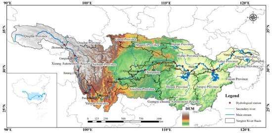
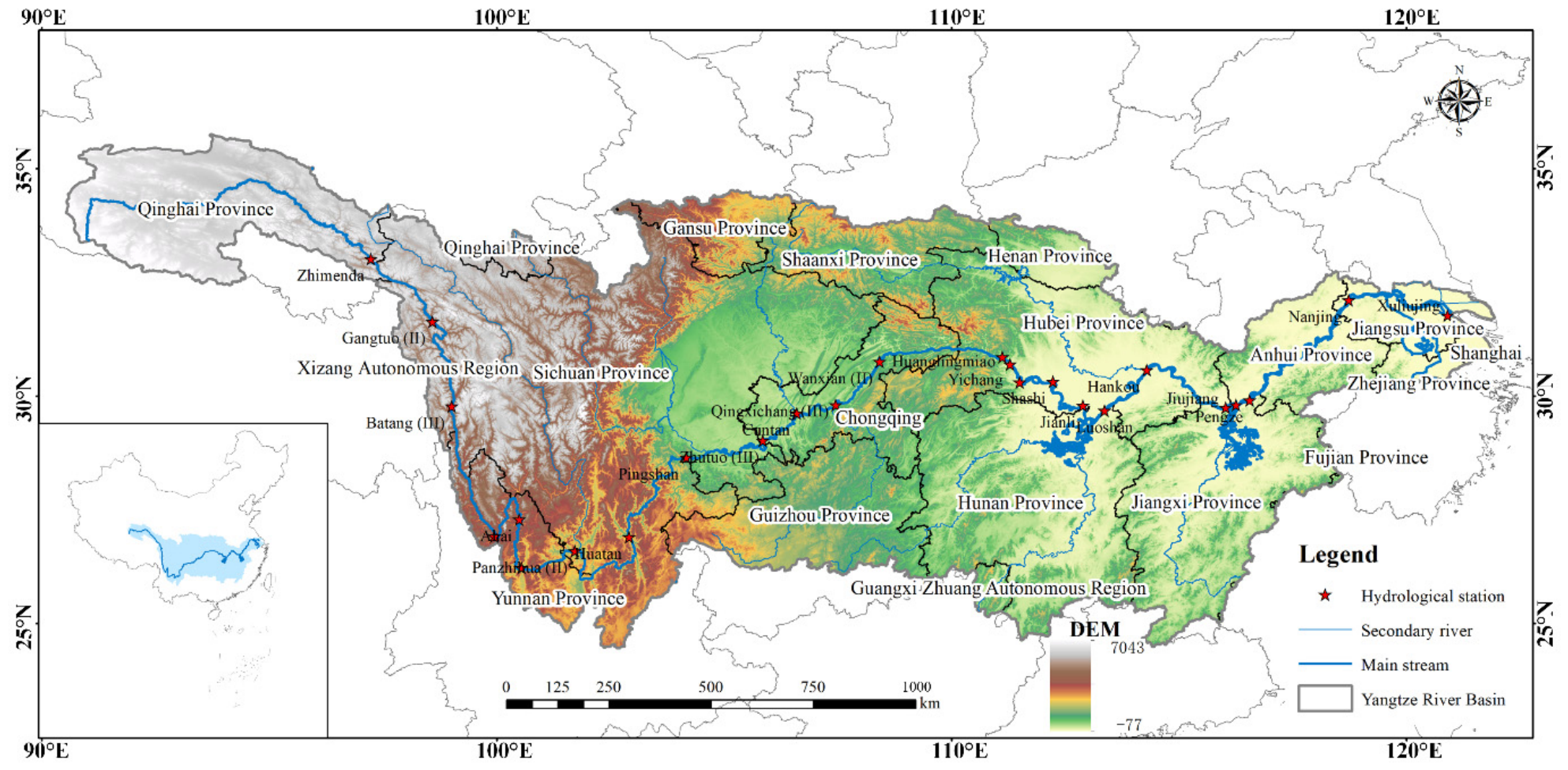
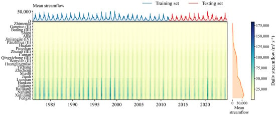
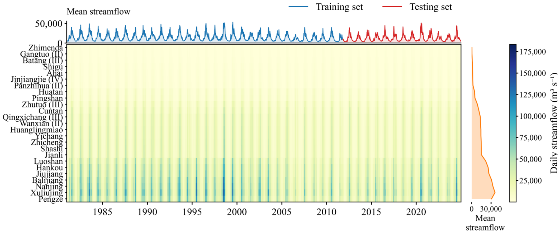
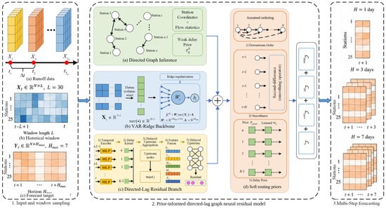
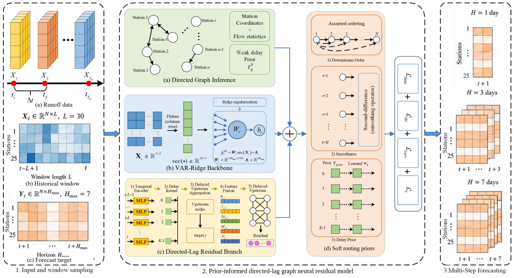
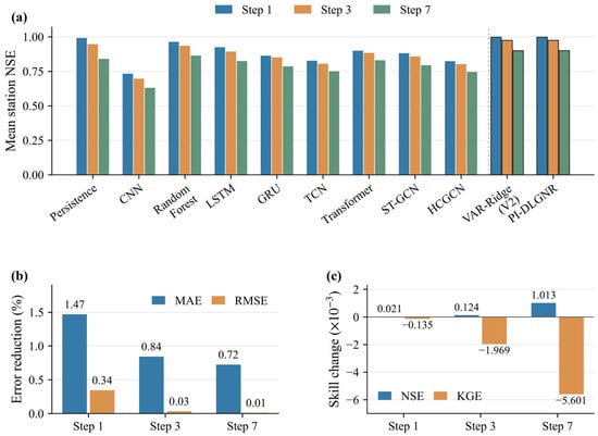
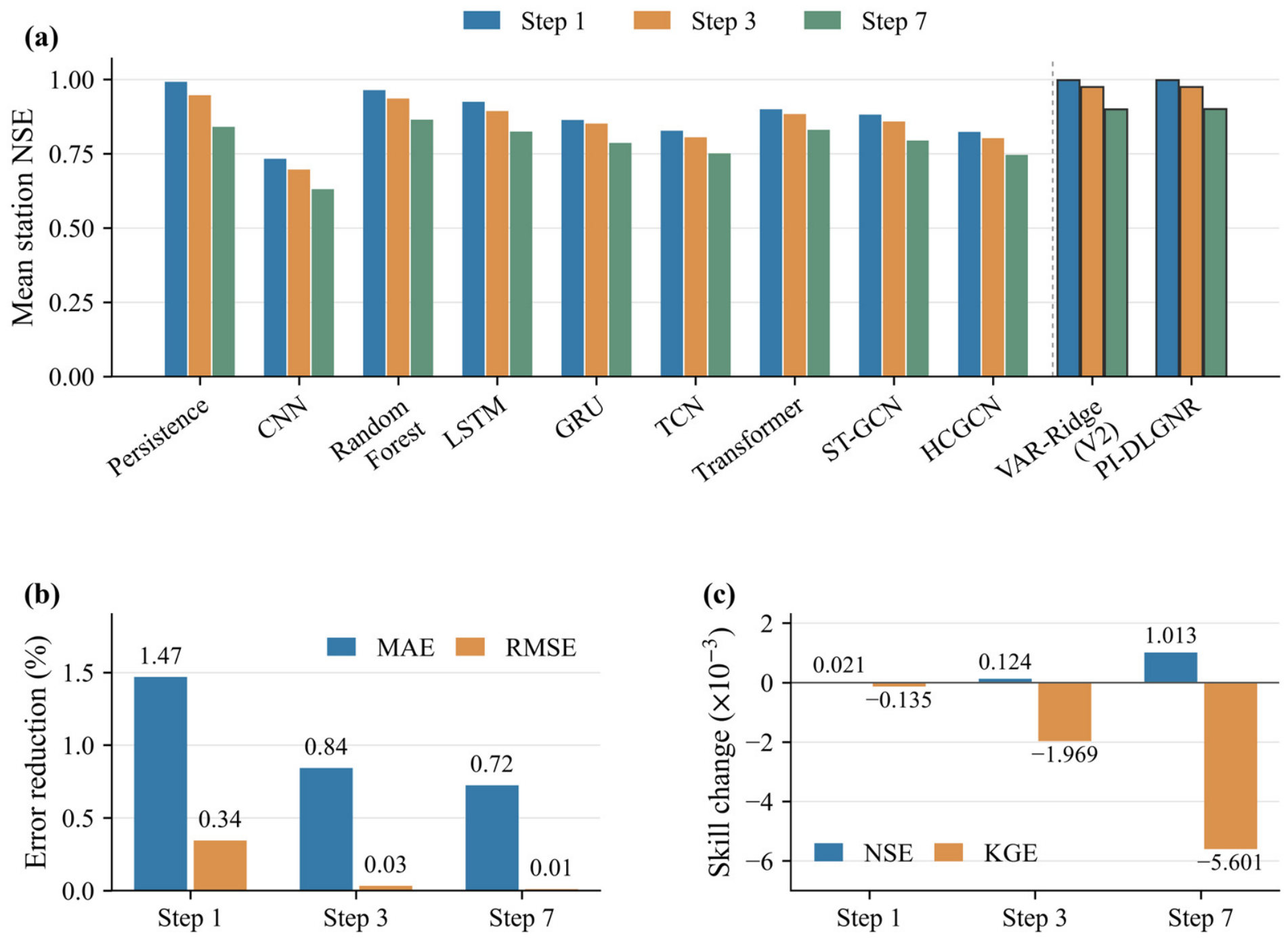
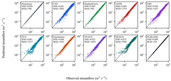
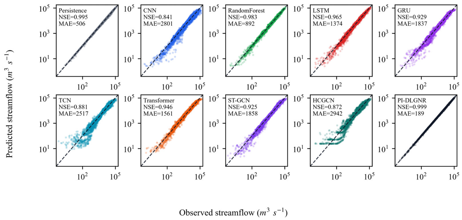
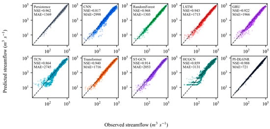
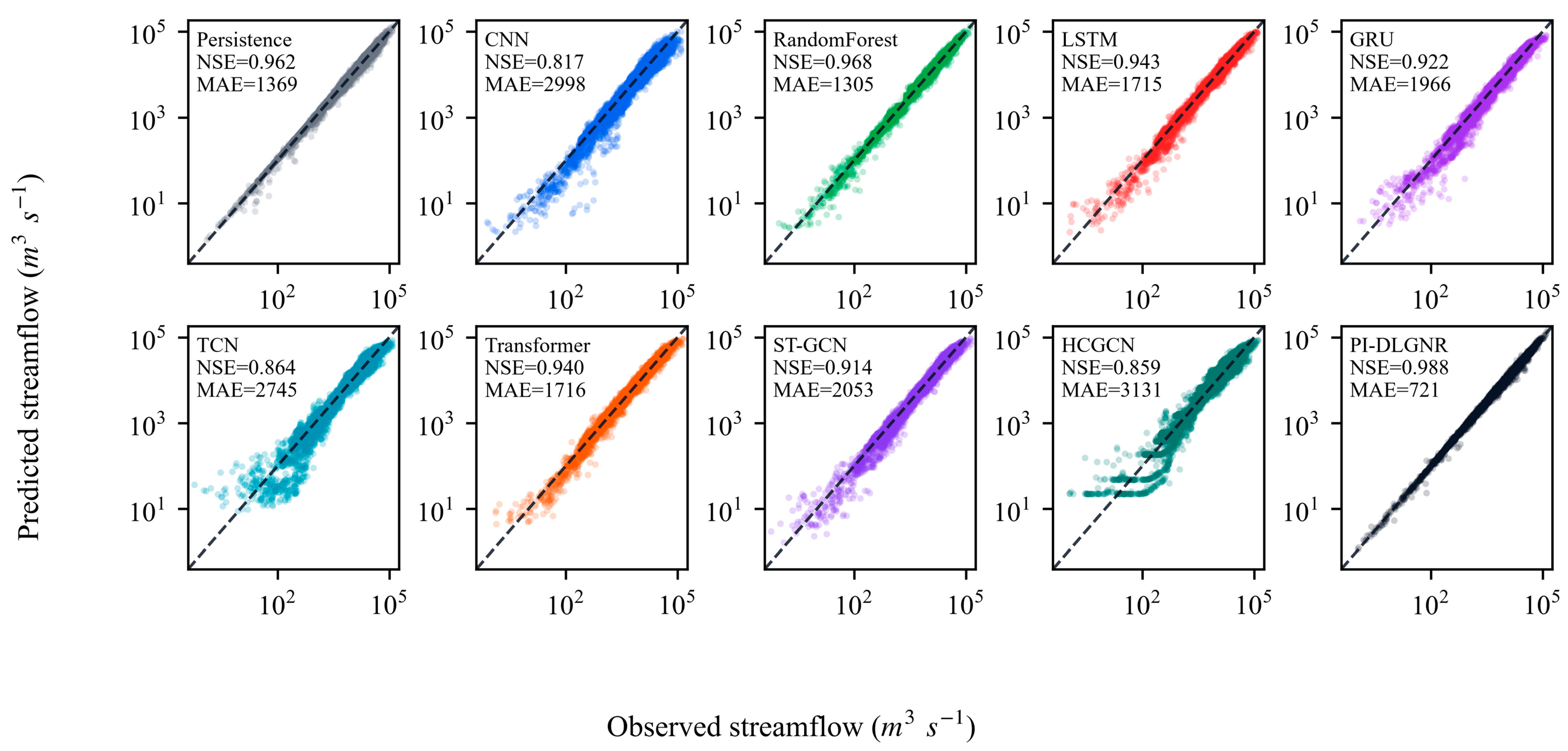
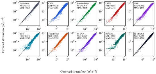
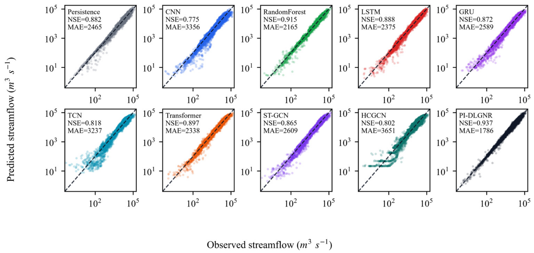
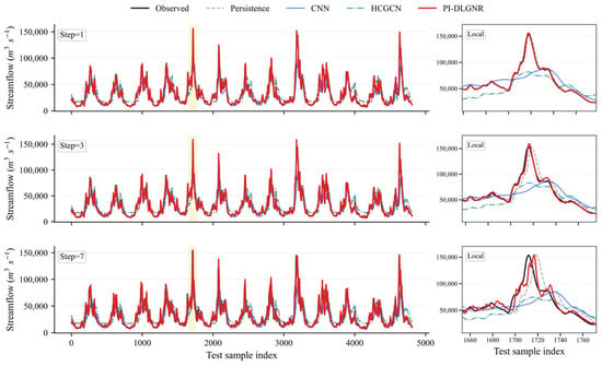
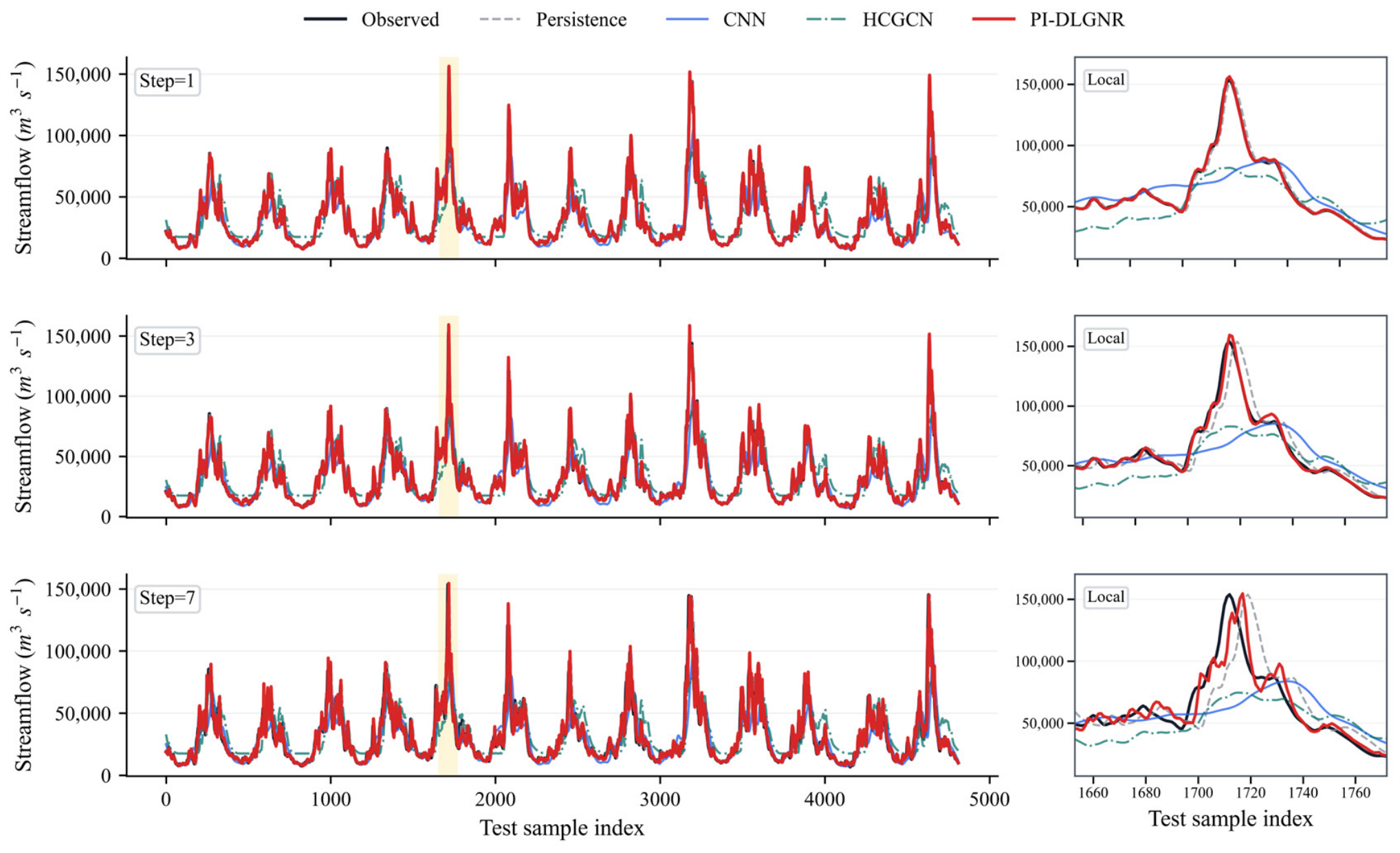
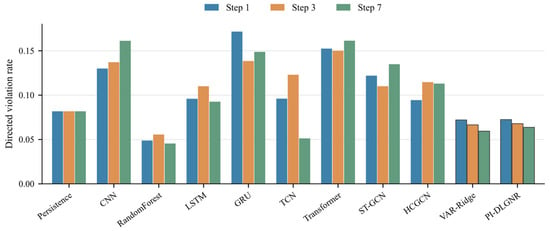
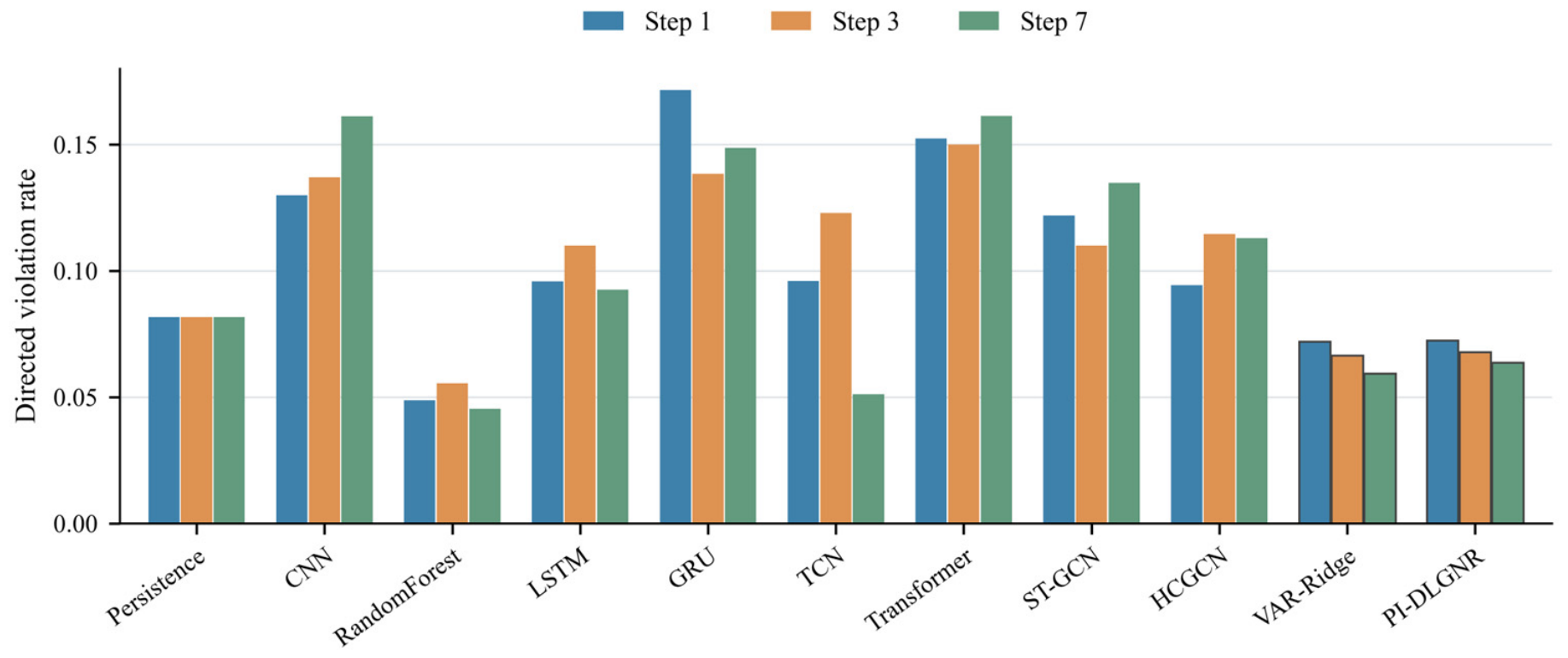
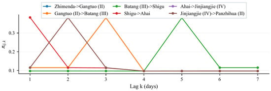
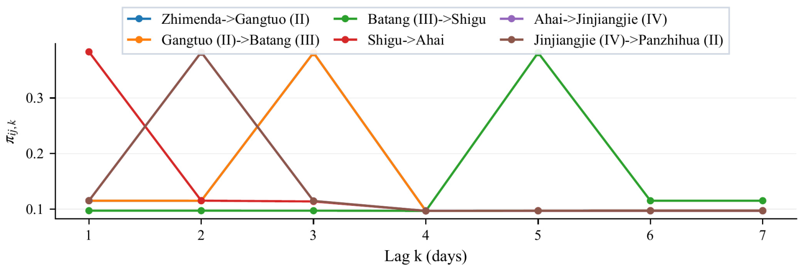
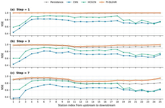
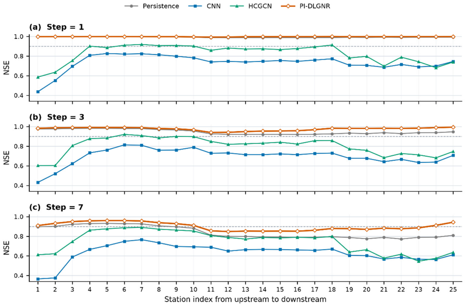
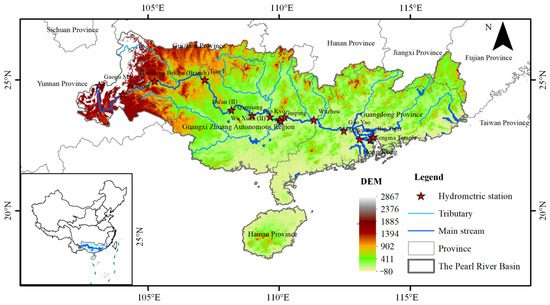
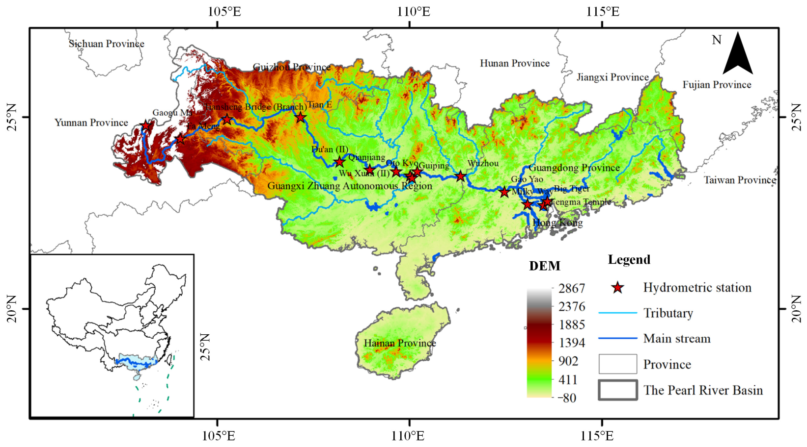
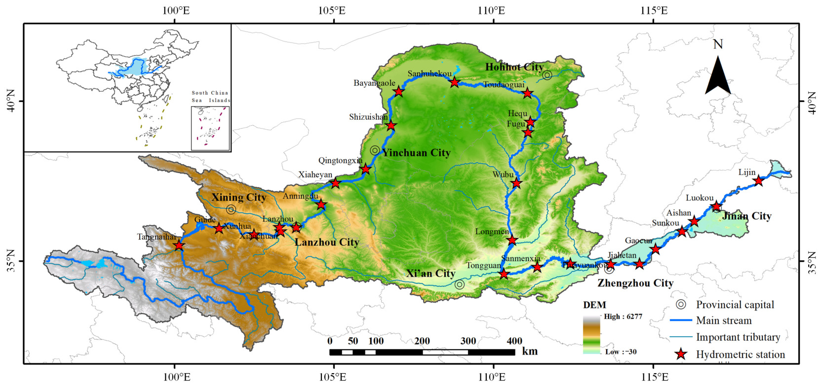
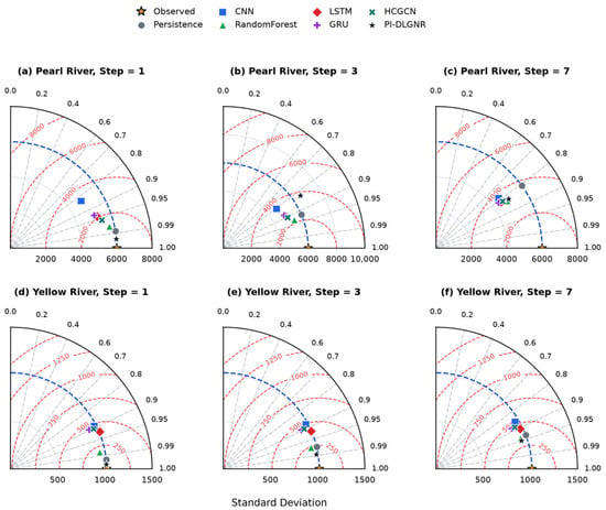
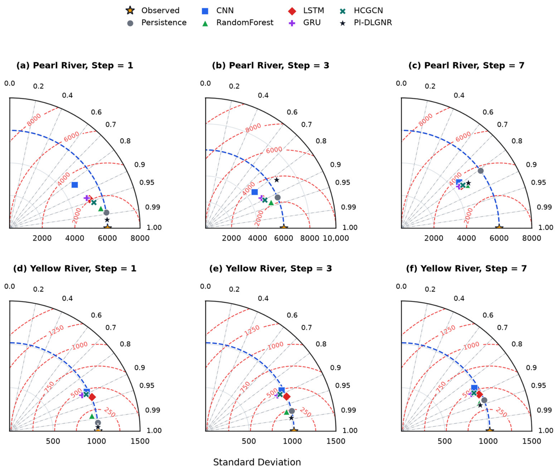
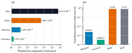
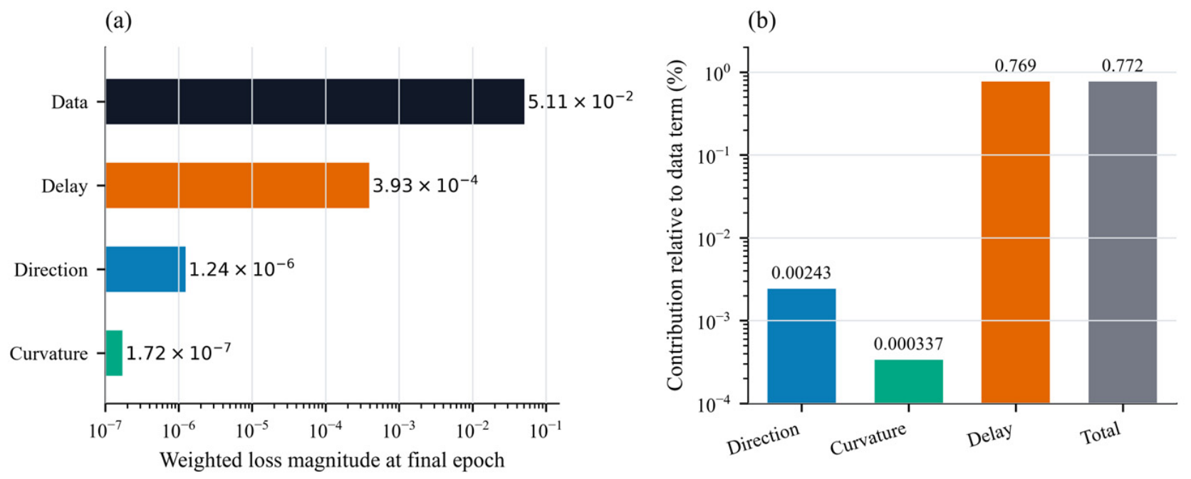

Disclaimer/Publisher’s Note: The statements, opinions and data contained in all publications are solely those of the individual author(s) and contributor(s) and not of MDPI and/or the editor(s). MDPI and/or the editor(s) disclaim responsibility for any injury to people or property resulting from any ideas, methods, instructions or products referred to in the content. |
© 2026 by the authors. Licensee MDPI, Basel, Switzerland. This article is an open access article distributed under the terms and conditions of the Creative Commons Attribution (CC BY) license.