Nonlinear Rational Method: Peak Discharge and Hydrograph Computation Without the Time of Concentration

Abstract

Lumped hydrological modeling approaches based on the Rational Method (RM) continue to be used in engineering practice despite the advent of various sophisticated hydrological modeling tools in the past decades. While the simplicity, low data requirements, and intuitiveness of the RM explain its longevity, many simplifying assumptions and uncertainties make its successful use difficult. Time of concentration (T_c) estimates, for instance, can vary up to 500% and lead to large discrepancies in rainfall intensity computations. We propose the Nonlinear Rational Method (NRM), which combines the low data requirements of the RM for rainfall abstraction with the Nonlinear Reservoir Algorithm to route overland flows while searching for a critical rainfall duration for the maximum peak discharge of the outflow hydrograph, thereby avoiding the need to compute T_c. The NRM is compared against the Storm Water Management Model (SWMM) and the RM-based Peak Flow Search Approach (PFSA). NRM peak discharges were within 15% of SWMM predictions in a systematic analysis of 12 synthetic subcatchments and within 2% of peak flows in a realistic watershed. The NRM was also compared with experimental datasets, indicating its ability to correctly reproduce peak flows. The ability to represent dissimilar subcatchments and to compute peak discharges without uncertainties from T_c makes the NRM an attractive choice for smaller urban catchment hydrological designs.

1. Introduction

A fundamental application of hydrological studies is determining peak discharges in urban watersheds linked with intense rain events. The development of approaches that provide estimates of peak discharges and hydrographs associated with intense rain events has spanned more than a century, and over time these approaches became increasingly more sophisticated. From semi-empirical approaches that lump key characteristics of drainage areas into fully discretized gridded models, there was an effort to improve the representation of rainfall–runoff transformation through better physical hydrological processes. For instance, semi-distributed or gridded models applying one- and two-dimensional formulations [1,2,3,4] have been used to resolve detailed spatial and temporal patterns of the rainfall–runoff processes. Some of these tools, such as the Storm Water Management Model (SWMM) [5], have been widely used in sizing drainage infrastructure.

Adoption of sophisticated hydrological modeling tools in engineering practice, however, remains uneven and limited. Common barriers include data-intensive inputs (e.g., high-resolution topography, soil parameters, land-cover classification), technical expertise needed to set up and calibrate the models, and licensing costs, among others [6]. As a result, lumped and semi-empirical methods continue to be popular for drainage design, particularly for the small drainage areas to which the Rational Method (RM) is applied; for example, the ALDOT Hydrology Manual [7] recommends the Rational Method (RM) for drainage areas smaller than 80 ha (200 acres), where low data requirements, conceptual transparency, and rapid execution outweigh the loss of physical detail.

Among these conceptually simpler methods, the Rational Method and its derivatives are among the most widely applied methods for small drainage designs because of their low data requirement and intuitiveness [8]. First proposed by Mulvaney [9] and formalized for urban applications by Kuichling [10], the method estimates peak runoff as the product of a runoff coefficient $C$, a representative rainfall intensity $i$, and the contributing drainage area $A$. Over the many decades since its application, practitioners have recognized the simplifying assumptions linked to the RM. These include spatiotemporal rainfall uniformity, spatiotemporal uniformity of abstraction (i.e., fixed C), and a single critical rainfall duration equal to the subcatchment time of concentration (T_c) for determining the runoff peak discharge (Q_p).

Among the significant modifications to the application of the RM was the frequency adjustment factor C_f for the runoff coefficient C. This factor, which is above unity, was introduced by Wright-McLaughlin [11], and assumes that abstractions become proportionally smaller during severe events. A more fundamental reinterpretation came from Guo and Urbonas [12], who redefined C as a volume-based ratio between runoff hydrograph volume and rainfall hyetograph volume rather than a peak-flow ratio. Their formulation derives C analytically using a ratio of the identified key factors of depression storage and infiltration losses normalized by the design rainfall depth. Efforts by Dhakal et al. [13] for Texas watersheds and Froehlich [14] for return-period-dependent coefficients have shown that empirically derived C values will vary from textbook tables or design manuals.

Whereas the RM aims to provide a peak discharge for small drainage conveyance designs, the Modified Rational Method (MRM) [15] expanded the method to derive simplified hydrographs. The MRM assumes that the drainage area runoff contributions grow linearly with time when there is a storm of duration D ≤ T_c, yielding a triangular-shaped hydrograph when D equals T_c and a trapezoidal-shaped one otherwise. Smith and Lee [16] subsequently reinterpreted the MRM as a conceptual extension of the original method, deriving its hydrograph shape from an explicit assumption of linear concentration of the contributing drainage area. Therefore, the MRM uses T_c not only for determining/specifying the critical design rainfall duration but also as a routing parameter to affect/control hydrograph shapes. More recently, approaches were proposed to separately route the runoff of sub-drainage areas with different times of concentrations (T_c values). Such an approach was formalized through the Peak Flow Search Approach (PFSA) [17], which was shown to yield peak discharges significantly higher than alternatives that average runoff coefficients from areas with dissimilar land use types. The key innovation of the PFSA is that the PFSA does not assume a critical design rainfall duration in advance (e.g., duration of T_c in the RM and the MRM) but instead searches for it: the rainfall duration $\tau$ is systematically varied between 5 and 60 min with one minute increments, the corresponding rainfall intensity value is retrieved from the local IDF curve, and peak discharge is determined using the MRM for each duration; through the search, the maximum peak discharge and corresponding rainfall duration are finally reported as PFSA results for the drainage conveyance design. The PFSA does not use T_c for directly specifying the critical design storm but still uses T_c for generating the MRM’s hydrograph for each subcatchment and then T_c values for all subcatchments still affect the maximum peak discharge for the whole drainage area.

All existing RM-family approaches depend on estimates for the time of concentration T_c within a watershed to define the critical design rainfall duration, and conventionally T_c is defined as the time required for runoff to travel from the contributing area’s most hydraulically remote point to the outlet. Despite its centrality to peak-flow design, the multiple empirical and semi-empirical formulas in use for T_c can produce strikingly different estimates for the same basin. Grimaldi et al. [18] examined four small basins and showed that estimates from common T_c methods could differ by up to 500 percent. Fang et al. [19] compared five widely used empirical formulas across 96 Texas watersheds and observed substantial differences in computed T_c values, with the choice of estimation formula introducing more variability than the choice of automated versus manual watershed-parameter extraction. McCuen [20] cataloged multiple computational definitions of T_c in the literature and quantified the resulting uncertainty in peak-flow estimates. Gericke and Smithers [21] attributed up to 75 percent of peak-flow error at the watershed scale to errors in the estimation of watershed response-time parameters. Because the choice of T_c formula is rarely subject to local calibration, this uncertainty is often carried forward unchallenged into design practice. Such strong dependency on times of concentration poses difficulties in using either RM or its variations since the peak discharges are strongly dependent on this parameter. Work by Simpson et al. [22] showed that direct calibration of the RM against observed rainfall–runoff data from a single flow-monitoring station can substantially improve peak-flow estimates, whereas adjustments based on higher-resolution soil, land-use, and topographic input data alone did not systematically improve performance. This finding suggests that persistent errors in RM-family methods stem as much from the structural assumptions of the method as from input-data resolution, reinforcing the case to explore methods that reduce the structural dependence on T_c.

Physically based hydrological models do not need an assumption for T_c as the overland flow hydrograph is predicted with overland flow equations. The SWMM, for instance, applies the Nonlinear Reservoir Approach (NRA) to convert rainfall excess time series into overland flow at the subcatchment scale using the flow continuity equation implementation and the Manning equation. The SWMM’s NRA data requirement includes drainage area, flow path length, slope, and roughness. Such formulation requirements are low when compared to formulations using gridded hydrological modeling tools for describing overland flows. Before implementing the NRA, the SWMM needs users to provide rainfall hyetograph and select one of the rainfall loss methods, e.g., depression storages on pervious and impervious areas, evaporation estimate, Horton’s method (three or five input parameters for event or continuous simulation), Modified Horton’s method, Green-Ampt Method (three parameters), and Curve Number Method (CN and drying time) [5]. Therefore, the SWMM is more complex in rainfall abstractions than lumped hydrological models; however, the relative simplicity of the NRA framework offers an opportunity to derive a T_c-agnostic approach for lumped hydrological models.

The objective of this work is to create a new discretized RM approach with the PFSA’s critical storm searching method and the NRA framework to prescind the calculation of T_c in the computation and to determine runoff peak discharge and associated hydrograph for small drainage design. The proposed method, the Nonlinear Rational Method (NRM), retains the RM’s simplicity by using the runoff coefficient to represent abstraction and the use of rainfall derived from IDF curves. The NRM, analogous to the PFSA [17], determines rainfall abstraction and performs the NRA separately for each subcatchment with different land use.

Rather than introducing new abstraction or routing methods, or a new critical-duration search algorithm, the NRM integrates existing methods in an approach that avoids the computation of the time of concentration. Specifically, the NRM utilizes the typical rate-based runoff coefficient C used in most RM-based calculations, the NRA overland flow routing algorithm from the SWMM, and a PFSA-style critical storm duration search for multiple subcatchments. The result is a method that retains the low data requirement of the RM, while producing physically based hydrographs without T_c computation.

The proposed NRM is benchmarked against PFSA and SWMM predictions of overland flows to compare its predicted hydrological results for selected cases involving various catchment characteristics and multiple subcatchments with dissimilar land uses. The following section outlines the methodology of the proposed approach, followed by a results section in which the NRM is benchmarked against the SWMM and PFSA. The work concludes with the discussion and conclusions.

2. Materials and Methods

2.1. NRM Mathematical Formulation

NRM treats every subcatchment or sub-drainage area as a nonlinear reservoir following the formulation presented in Chapter 3 of the SWMM Reference Manual [5]. For a subcatchment $j$ with contributing area $A_j$, runoff coefficient $C_j,$ subcatchment width $W_j$, flow path slope $S_{oj}$, and Manning’s roughness coefficient $n_j$, the ponded depth $d_j$ can be computed through the continuity equation in a reservoir involving nonlinear processes:

$$\begin{gathered} {\displaystyle \frac{d{d}_j}{dt}} = i_e\left(\tau \right) - q_j\left(d_j\right) \\ {\displaystyle \frac{d{d}_j}{dt}} = C_j i\left(\tau \right)\left[1-H\left(t-\tau \right)\right]-q_j\left(d_j\right) \end{gathered}$$

(1)

where $i\left(\tau \right)$ is the rainfall intensity derived from the IDF curve, $i_e$ is the rainfall excess, and $q_j$ is the outflow per unit area. The rainfall excess is equal to $C_j\cdot i\left(\tau \right)$ for the rain duration and is zero afterward, hence the Heaviside function H($t-\tau$) = 0 after $t>\tau$; only the second term on the right-hand side of the equation remains, representing the subcatchment draining process.

The system of ordinary differential equations in Equation (1) is integrated numerically using an explicit forward Euler scheme, following Press et al. [23], implemented in MS Excel VBA. A uniform computational time step of $\mathsf{\Delta }t$ = 1 s is applied throughout the simulation, ending at 60 min. For each candidate storm duration τ (varied from 5 to 60 min in 1 min increments), the ponded depth d_j is set to zero for every subcatchment at t = 0, representing a design storm falling on a fully drained watershed. The selected $\mathsf{\Delta }t$ = 1 s was sufficient to ensure stability in all tested cases, and other values were not tested.

Runoff outflow from the subcatchment is computed using the SWMM kinematic-wave form with the alpha coefficient defined from Manning’s equation:

$$Q_j\left(d_j\right)=q_j\left(d_j\right)\cdot A_j = A_j\cdot {\alpha }_j · {\left(d_j\right)}^{5/3} with {\alpha }_j = {\displaystyle \frac{k{W}_j{S_{oj}}^{1/2}}{A_j{n}_j}}$$

(2)

The constant $k$ is equal to 1.0 for applications using SI and 1.49 for applications using USCS units. The watershed/drainage flow at any given time $t$ is the sum of each subcatchment outflow as shown in Equation (3), which then enables the development of hydrographs for subcatchments q_j(t) and the whole drainage area Q_tot(t).

$$Q_{tot}\left(t\right)=\sum _j{Q}_j\left(d_j\left(t\right)\right)$$

(3)

To preserve RM simplicity, instead of time-varying hyetographs, NRM uses a constant rainfall intensity value derived from IDF curves for a given design area. However, rather than assuming a critical rainfall duration, NRM follows the PFSA and computes the hydrographs and peak discharges using Equation (3) for varying rainfall durations $\tau$, e.g., between 5 and 60 min with one-minute increments. The search is limited to 60 min as some design guidelines (e.g., ALDOT Hydrology Manual [7]) adopt this limit, though larger catchments could require a larger maximum rainfall duration. The lower bound of 5 min reflects the practical limit at which most IDF curves are formulated with confidence, and the upper bound of 60 min is well beyond the time of concentration typically expected for small drainage areas up to 80 hectares (200 acres) [7]. For instance, if a Sherman-form intensity–duration–frequency (IDF) curve is used with coefficients $a$, $b$, and $m$ that depend on a given location and the selected design recurrence intervals:

$$i\left(\tau \right) = {\displaystyle \frac{a}{{\left(\tau + b\right)}^m}}$$

(4)

Thus, for each rainfall duration $\tau$, the rainfall intensity is calculated using Equation 4, and this intensity is used in the computation of depth and runoff outflow rates over time (i.e., Equation (1) to (3)). The PFSA searching approach will result in a critical rainfall duration that will maximize the peak discharge of the drainage area. The corresponding hydrograph and peak runoff flow can be used for conveyance and stormwater detention design. In addition to IDF data, the NRM requires five parameters per subcatchment: runoff coefficient $C$, Manning’s roughness $n$, slope $S$, flow path length $L$, and contributing area $A$. All such parameters are easily obtainable and consistent with many RM-based calculations. The NRM is for small drainage design to determine the maximum peak discharge for subcatchments with different land uses or C values. It is not for predicting or simulating hydrographs for event rainfalls and continuous rainfall events.

2.2. NRM Assessments

The performance of the NRM was evaluated through a sensitivity analysis and comparisons with the SWMM and PFSA under both controlled cases, a realistic watershed case, and experimental datasets.

•

Assessment 1 involved using twelve single-land-use subcatchments, each case with a varying combination of land cover and slopes, drawn from the Hydrology Manual of the Alabama Department of Transportation [7], as shown in Table 1. Values of rate-based runoff coefficients from this manual, referred to as $C_{ALDOT}$, and roughness $n$ were paired with three slope classes (flat = 2.5%, rolling = 7.5%, and hilly = 20%) as defined in the same manual. Each case was calculated with area A = 8000 m² (86,111 ft²), and flow path length L = 60 m (196.85 ft) so that peak discharge varied only with the given $C, n, \mathrm{a}\mathrm{n}\mathrm{d} S$ combination of interest. The design rainfall used Sherman IDF coefficients for the City of Opelika, Alabama.

Table 1. Inputs to Assessment 1. All twelve cases used L = 60 m (196.85 ft) and A = 8000 m² (86,111 ft²).

Parameter	Case 1	Case 2	Case 3	Case 4	Case 5	Case 6	Case 7	Case 8	Case 9	Case 10	Case 11	Case 12
ALDOT Table 4.4	Clay/silt loam woodland			Clay/silt loam pasture			Clay/silt loam cultivated			50% impervious urban		Concrete
Runoff Coefficient	0.3	0.35	0.5	0.3	0.36	0.42	0.5	0.6	0.72	0.55	0.65	0.8
Slope Class	Flat	Rolling	Hilly	Flat	Rolling	Hilly	Flat	Rolling	Hilly	Flat	Rolling	-
Manning’s n	0.10	0.10	0.10	0.035	0.035	0.035	0.040	0.040	0.040	0.050	0.050	0.017
Slope	0.025	0.075	0.20	0.025	0.075	0.20	0.025	0.025	0.20	0.025	0.075	0.01
Curve Number *	75.00	82.00	91.51	79.83	87.06	91.53	91.16	95.02	97.71	92.37	95.94	98.21
Kerby’s Tc Retardance Coefficient	0.20	0.20	0.20	0.10	0.10	0.10	0.10	0.10	0.10	0.10	0.10	0.02
$\mathrm{Runoff} \mathrm{Volumetric} \mathrm{Coefficient} \mathrm{from} \mathrm{SWMM} \mathrm{Output} \left(C_{SWMM}\right)$	0.141	0.193	0.346	0.161	0.215	0.299	0.336	0.464	0.629	0.374	0.507	0.739

* Curve Number values were dynamically computed using Equation (7) based on 56 rainfall durations from 5 to 60 min, and only the resulting CN corresponding to the critical durations obtained with SWMM computation that yield the maximum peak discharge from each case catchment is reported here. See Section 2.3 for more information.

•

Assessment 2 involved using a case presented in Yang [24] that aimed to apply the NRM in conditions of multiple subcatchments with dissimilar land uses near a soccer field in Birmingham, Alabama. The drainage area comprises five subareas of contrasting land use drained to a single outlet: a 2.12 ha clay–loam woodland with $C =$ 0.18; two grassed subareas of 1.78 ha and 0.90 ha with $C =$ 0.10; and two impervious areas of 0.36 ha and 0.15 ha with $C =$ 0.96, with overland flow path lengths ranging from 36.6 to 198.1 m.

•

Assessment 3 assesses NRM performance using experimental measurements of overland flows on two experimental studies that involved fixed rainfall intensities. Experiment 1 was presented by Yu and McNown [25] and included a test with 8 min of rainfall duration with 189 mm/hr intensity on a smooth concrete channel 152.4 m long and 0.3 m wide with a 2% slope, part of a series of airport-runway drainage experiments. Experiment 2, from Izzard and Augustine [26], included a rainfall event with 11 min of rainfall duration and 98.3 mm/hr intensity on a smoothly paved plot 21.9 m long and 1.8 m wide with a 0.1% slope, part of a Public Roads Administration and Soil Conservation Service cooperative research project [26]. In both cases, the subcatchments were rectangular with much longer flow path length than subcatchment width. Also, both datasets provide observed outflow hydrographs under controlled artificial-rainfall conditions on impervious surfaces, so the runoff coefficient C is effectively 1.0, and the runoff response is governed by the interaction among surface roughness, slope, geometry, and rainfall.

For Assessments 1 and 2, NRM calculations were run for the 5-year recurrence interval, and the resulting critical rainfall durations and design hydrographs were derived. These results were subsequently compared with the results obtained with the SWMM, as is detailed below. In addition, these results were compared with PFSA results calculated with the same conditions using the Velocity method [27] and the Kerby method [28] to compute the time of concentration.

2.3. SWMM Setup for NRM Comparison

Considering the differences between the SWMM and NRM, some adjustments to the SWMM input files were needed to enable a comparison between these two approaches:

•

SWMM’s parameter “Subcatchment Width” was set to $A / L$ to match the geometry adopted in NRM calculations.

•

SWMM’s subcatchment depression storage and evaporation were both neglected, and the only relevant abstraction considered was infiltration.

•

Infiltration was represented with the Curve Number (CN) approach as implemented in the SWMM [5].

•

The SWMM was run 56 times via VBA code for rainfall durations, ${\tau }_i$, from 5 to 60 min (in one-minute increments), to search for a critical rainfall duration that yields the maximum peak discharge from the catchment, obtained by combining all subcatchment runoff hydrographs.

Following Pitt [29], CN values were computed from the per-subcatchment Rational runoff coefficient C by direct algebraic inversion of the SCS runoff equation [30] after considering that the SWMM does not use the initial abstraction Ia but depression storage:

$$RD = {\displaystyle \frac{P^2}{P +SM}}$$

(5)

where P is the rainfall depth, RD is the runoff depth, and SM is the potential maximum retention, in consistent units. The maximum retention SM is related to the CN through Equation 6, represented below using the SI and USCS system of units:

$$\begin{gathered} SM(mm)= {\displaystyle \frac{\mathrm{25,400}}{CN}} - 254 \\ SM(in)= {\displaystyle \frac{1000}{CN}} - 10 \end{gathered}$$

(6)

For each subcatchment $j$, the design storm depth $P_i$ was computed from the IDF curve at all possible rainfall durations, ${\tau }_i$, between 5 and 60 min, $P_i = i\left({\tau }_i\right)·{\tau }_i$. The corresponding runoff depth was set to $R{D}_{i,j}=C_j·P_i$. Substituting Equation (6) into Equation (5), one can derive Equation (7) to compute the CN for the SWMM under USCS units:

$${CN}_{i,j}=1000{\displaystyle \frac{{RD}_{i,j}}{\left[{P_i}^2+10 {RD}_{i,j}-{RD}_{i,j}*P_i\right]}}$$

(7)

For each rainfall duration ${\tau }_i$, corresponding rainfall intensity $i\left({\tau }_i\right)$ and depth $P_i$ are obtained, and thus a set of $C{N}_{i,j}$ is computed for each subcatchment $j$ for runoff computations within the SWMM. The identified critical rainfall duration (${\tau }_{crit}$) from the SWMM may be different from the critical duration $\tau$ obtained through the NRM peak runoff algorithm described in Section 2.1.

A subcatchment with a short rainfall duration sees a small $P$ and is therefore assigned a higher $CN$ than the same surface would receive at a large $P$ (a long rainfall duration). This treatment is conceptually consistent with Pitt’s [29] observation that runoff response in the small-storm depth range characteristic of urban design events is strongly depth-dependent. The CN values produced by Equation 7 vary across locations and return periods for the same land cover because $P_j$ depends on both the IDF coefficients of the design location and the design recurrence interval. Calculated CN values for the 12 test cases at their resultant ${\tau }_{crit}$, obtained from the SWMM, are given in Table 1.

3. Results

3.1. Assessment 1: ALDOT Twelve-Case Comparison

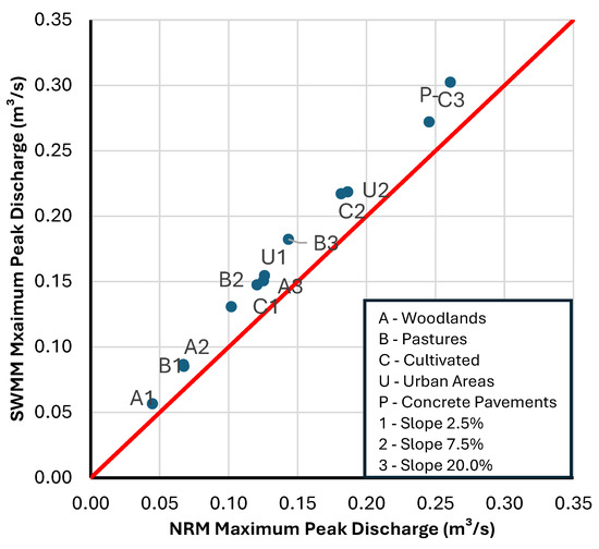
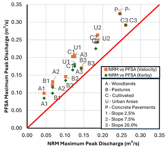
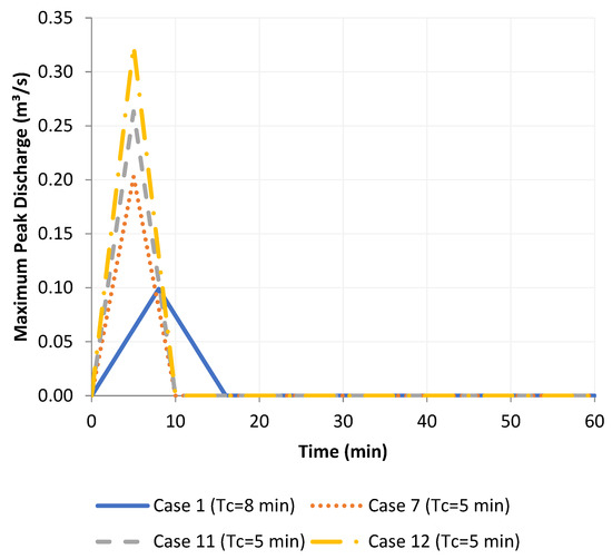
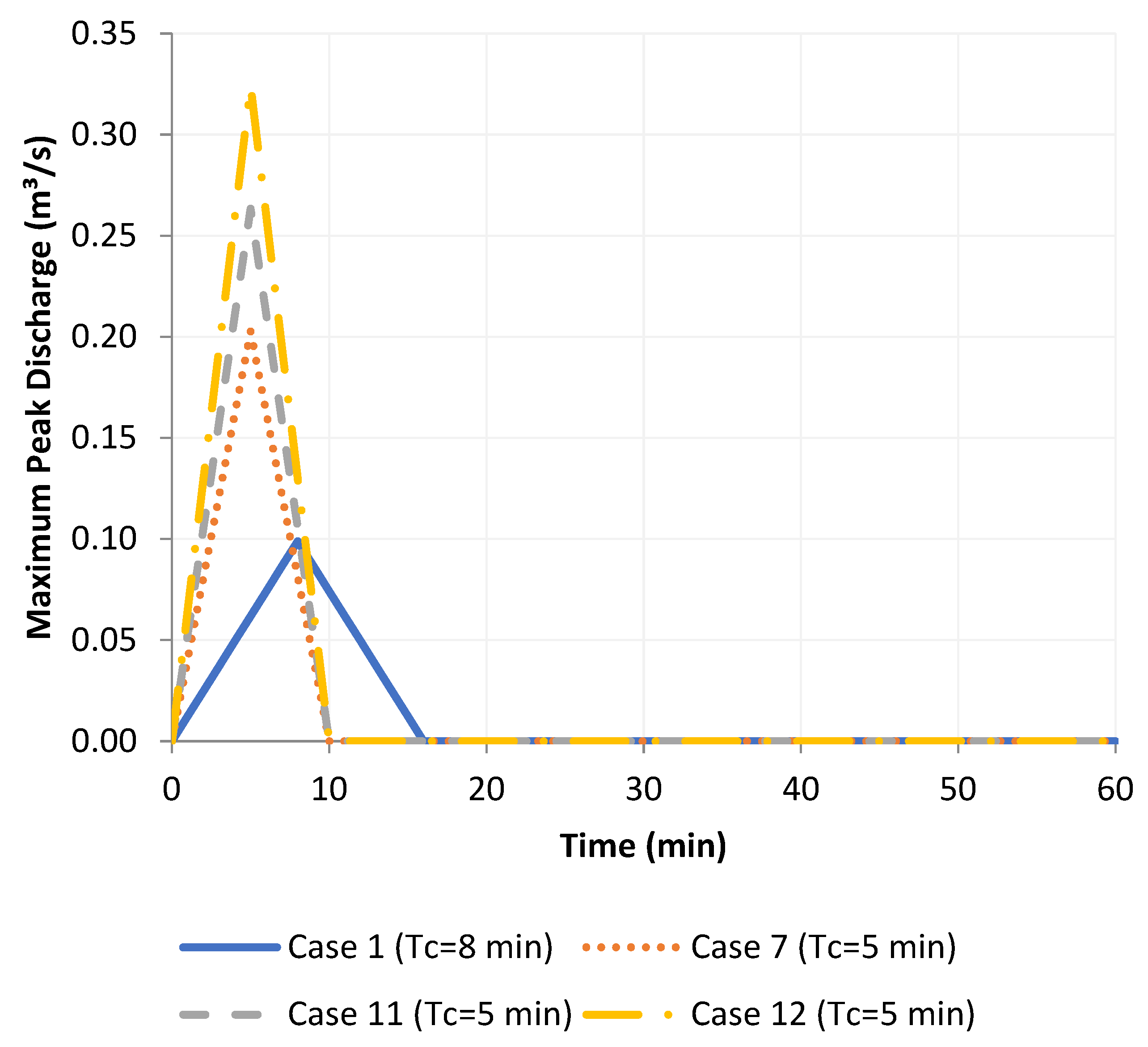
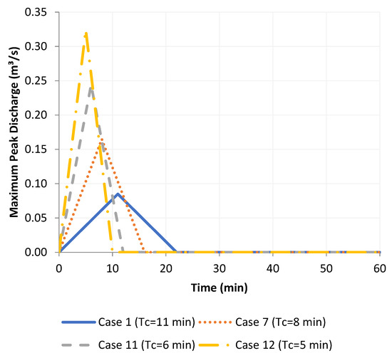
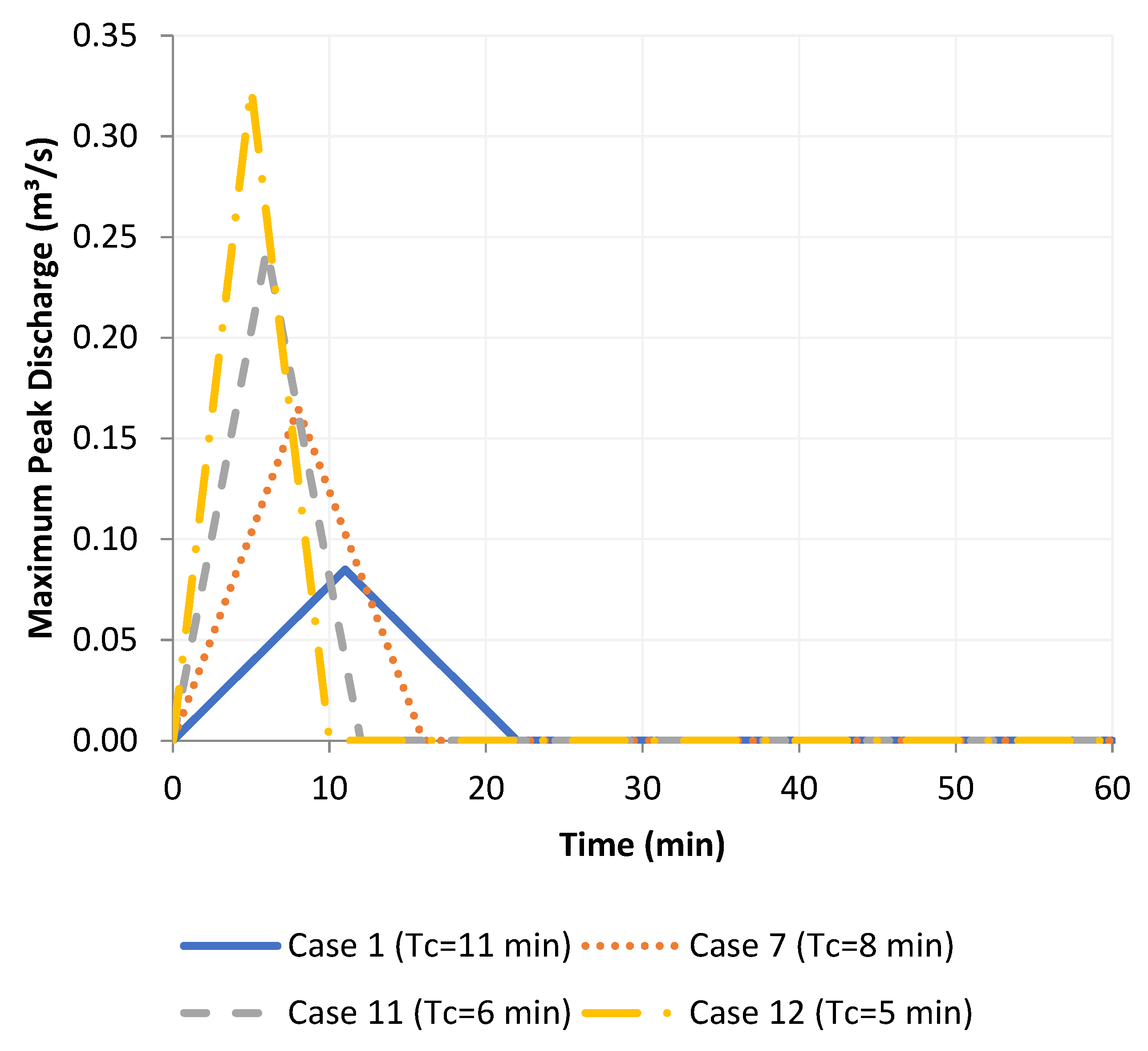
Maximum peak discharges for the twelve cases for Assessment 1 were computed with NRM, SWMM, and the PFSA using $T_c$ based on the Velocity and Kerby’s methods, with results summarized in Table 2, including the time of peak ($T_p$) runoff flows, and compared in Figure 1 and Figure 2. For all these approaches, the rainfall duration $\tau$ was systematically varied between 5 and 60 min, and the corresponding rainfall intensity values were retrieved. For each approach, the maximum peak discharge was determined, along with a critical rainfall duration and associated outflow hydrographs, and the model results were benchmarked. For Assessment 1, each case is for a single subcatchment or drainage area; therefore, $T_p$ for the outflow hydrograph is the same as the rainfall duration $\tau$ (see Figure 3 and Figure 4). For the PFSA method for a single subcatchment, $T_p$, the critical rainfall duration, and T_c are the same (see Figure 5 and Figure 6).

Table 2. Assessment 1 per-case maximum peak discharge and time of peak from NRM, SWMM, and the PFSA computed with two time-of-concentration methods (Velocity and Kerby) across the twelve ALDOT cases. The codes (e.g., A1) are used in Figure 1 and Figure 2.

Case and Codes	Maximum Peak Discharge Qp (m3/s)				${\mathit{\tau }}_{\mathit{c}\mathit{r}\mathit{i}\mathit{t}}$ for NRM & SWMM or Tc for PFSA (min)
	NRM	SWMM	PFSA Vel.	PFSA Kerby	NRM	SWMM	PFSA Vel.	PFSA Kerby
1—A1	0.045	0.057	0.099	0.085	22	27	8	11
2—A2	0.068	0.085	0.131	0.115	14	18	6	8
3—A3	0.126	0.155	0.203	0.175	9	11	5	7
4—B1	0.067	0.087	0.122	0.099	11	15	5	8
5—B2	0.102	0.131	0.146	0.135	7	9	5	6
6—B3	0.143	0.182	0.170	0.170	5	6	5	5
7—C1	0.121	0.148	0.203	0.165	10	12	5	8
8—C2	0.182	0.217	0.243	0.225	6	8	5	6
9—C3	0.261	0.302	0.292	0.292	5	5	5	5
10—U1	0.125	0.151	0.206	0.181	11	13	6	8
11—U2	0.186	0.219	0.263	0.244	7	8	5	6
12—P-	0.245	0.272	0.324	0.324	6	7	5	5

Figure 1. Assessment 1—maximum peak discharge comparison of NRM against SWMM for the twelve ALDOT cases. The red line is the 1:1 reference.

Figure 2. Assessment 1—maximum peak discharge comparison of NRM against PFSA computed with the NRCS Velocity and Kerby time-of-concentration methods for the twelve ALDOT cases. The red line is the 1:1 reference.

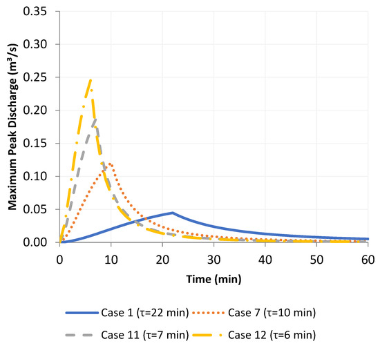
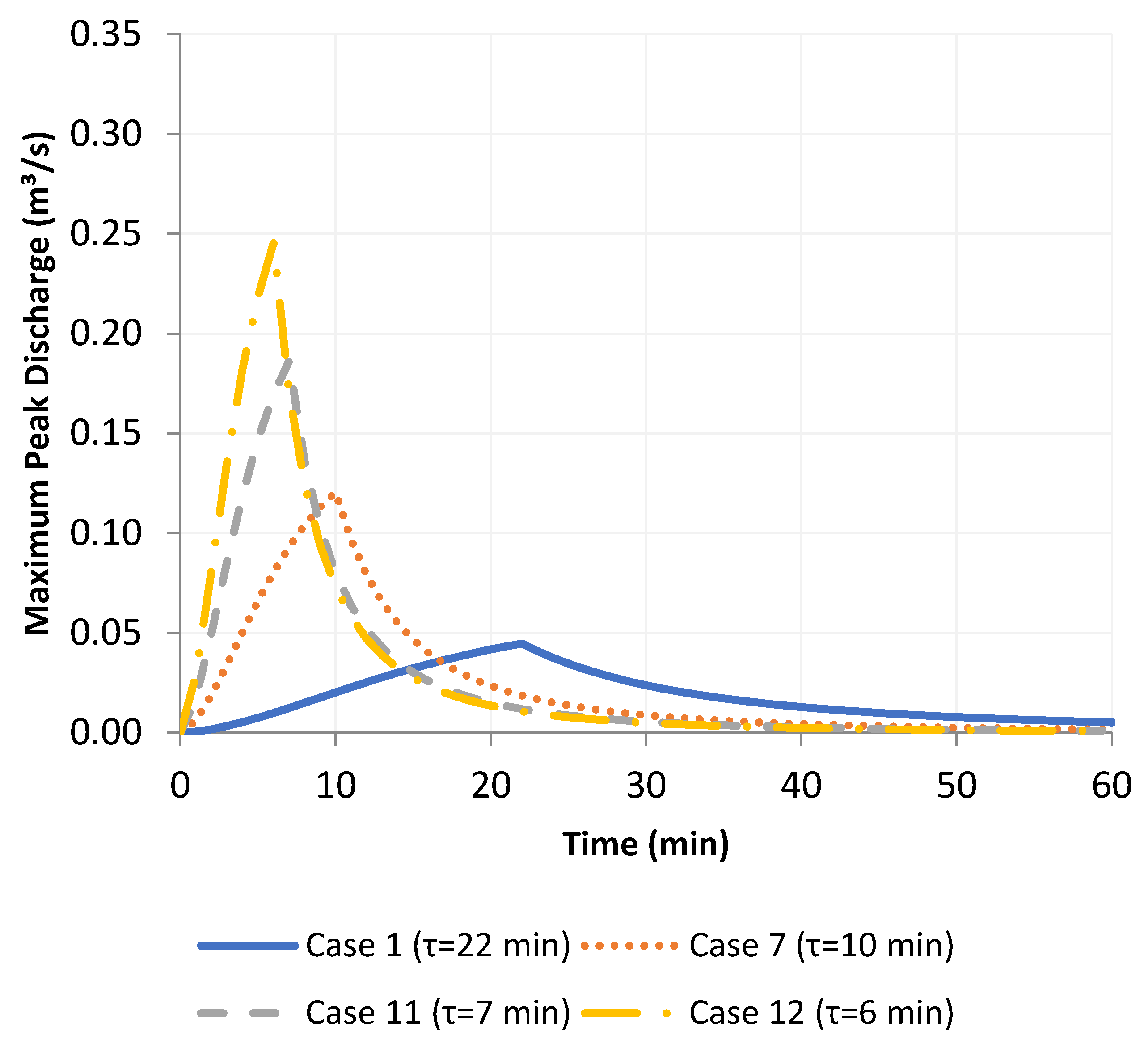
Figure 3. Assessment 1—NRM outflow hydrographs for four representative subcatchments (Cases 1, 7, 11, 12); the critical rainfall duration ${\tau }_{crit}$ determined by the NRM search is annotated on each series.

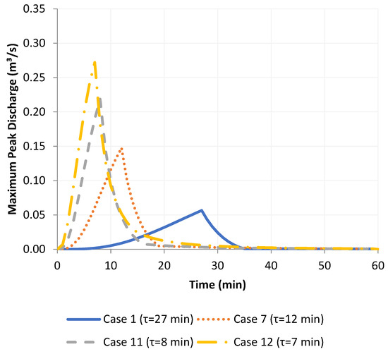
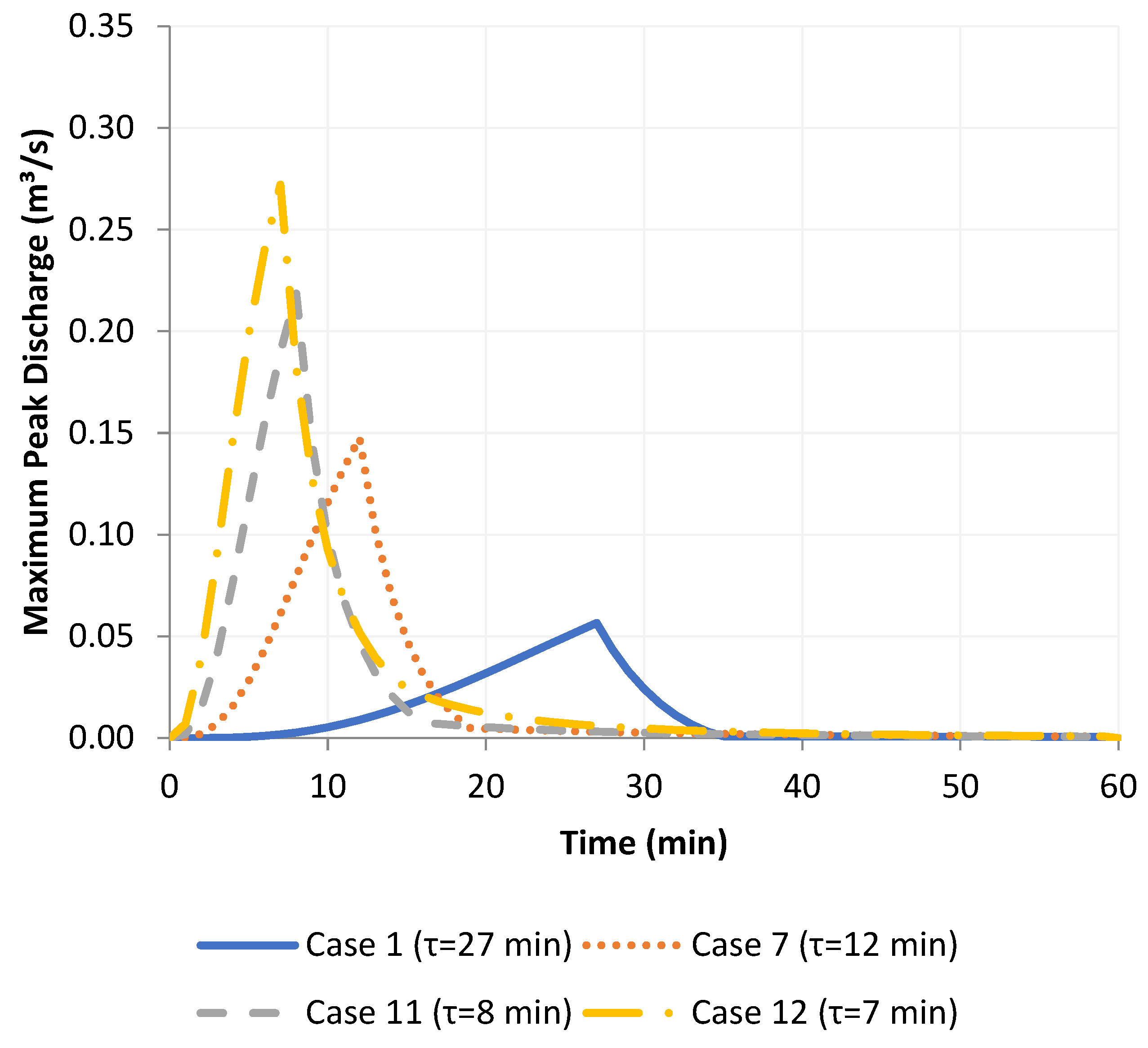
Figure 4. Assessment 1—SWMM outflow hydrographs for the same four subcatchments (Cases 1, 7, 11, and 12) driven at their SWMM critical rainfall durations.

Figure 5. Assessment 1—PFSA outflow hydrographs computed with the NRCS Velocity T_c method for the same four subcatchments (Cases 1, 7, 11, and 12).

Figure 6. Assessment 1—PFSA outflow hydrographs computed with the Kerby T_c method for the same four subcatchments (Cases 1, 7, 11, and 12).

A scatter plot of NRM peak runoff flows against the SWMM peak is presented in Figure 1, with close NRM and SWMM agreement across all twelve cases. A dimensionless ratio between peak discharges Q_SWMM/Q_NRM had a mean of 1.22 with values ranging from 1.11 to 1.29, and the NRM vs. SWMM scatterplot in Figure 1 yielded a slope of 1.097 and a coefficient of determination R² = 0.994. The largest SWMM-versus-NRM disagreement occurred with the cases with the lowest runoff coefficients. The smallest disagreement was observed at the concrete pavement case. The pattern of a larger peak ratio for the SWMM vs. NRM is consistent with larger volumetric runoff coefficients that were computed by the SWMM following the conversion of $C_{ALDOT}$ into the CN using Equation (7).

Similarly, NRM and PFSA peak runoff flow results were compared in Figure 2 and indicate that PFSA results are substantially larger. The dimensionless ratio Q_PFSA/Q_NRM had a mean of 1.78 with values ranging from 1.55 to 2.24, so PFSA peaks exceeded the corresponding NRM peaks by 55% to 124%. The PFSA peaks in Table 2 were systematically larger than both NRM and SWMM peaks across all twelve cases, with the results from the Velocity method $T_c$ typically higher than ones from Kerby $T_c$ across all twelve cases: the PFSA’s critical rainfall durations were the shortest (5 to 8 min for Velocity $T_c$, 5 to 11 min for Kerby $T_c$), followed by the NRM (5 to 22 min), then the SWMM (5 to 27 min). NRM times to peak runoff were comparably smaller than SWMM values, possibly reflecting the differences between the simplified abstraction adopted by the NRM and the more complex time-varying SWMM abstraction using the CN, which continues until the subcatchment depth reaches 1.3 mm (0.05 in). While the NRM and PFSA use the same simplified abstraction (i.e., runoff coefficient), they have different routing methods: the NRM’s is nonlinear reservoir routing, and the PFSA has a linear relation to the contributing area, as in the case of the MRM.

The consistently smaller PFSA times for peak flows are consistent with the PFSA’s use of the MRM assumption of linear concentration of the tributary area. Because IDF rainfall intensity decreases at a faster rate than the linear growth of drainage areas assumed by the MRM, the PFSA solutions are drawn toward shorter $T_c$ values. For the NRM, however, while larger $\tau$ values imply smaller rainfall intensities derived from IDF data, the subcatchment depth and related outflows increase with $\tau$, as shown in Equation (1). While a very large $\tau$ typically will not be linked with maximum peak discharge condition, an equilibrium depth would be observed in an NRM subcatchment calculated if it experienced a long-duration rainfall with fixed intensity $i\left(\tau \right)$:

$${\displaystyle \frac{d{d}_j}{dt}}\approx 0\to 0=C_j\cdot i\left(\tau \right)-{\displaystyle \frac{k\sqrt{S_{oj}}}{L_j{n}_j}} · {\left(d_{eq,j}\right)}^{{\displaystyle \frac{5}{3}}}\to d_{eq,j}={\left[\frac{C_j\cdot i\left(\tau \right)\cdot n_j\cdot L_j}{k\sqrt{S_{oj}}}\right]}^{3/5}$$

(8)

The hydrographs for four of the twelve cases corresponding to the maximum peak runoff flows were calculated and are shown in Figure 3, Figure 4, Figure 5 and Figure 6 and were selected as they yielded varying intensities of peak runoff flow discharges. Figure 3 and Figure 4 present the hydrographs from the NRM and SWMM solutions, respectively. Since the Nonlinear Reservoir Algorithm is used for runoff routing in NRM and SWMM solutions, their hydrographs have nonlinear increases to peak discharges and then nonlinear decreases (Figure 3 and Figure 4). It can be noted that NRM and SWMM hydrographs have comparable maximum peak discharges and time for peak flows, though SWMM peaks tend to occur slightly later. Figure 5 and Figure 6 present outflow hydrographs for the PFSA cases using the Velocity $T_c$ and Kerby $T_c$, respectively. The PFSA hydrograph shapes are triangular, given that each case corresponds to a single type of land use, thus consistent with the MRM solutions. The peak discharges from the PFSA paired with the Velocity $T_c$ are larger than the ones obtained with the Kerby $T_c$ solutions.

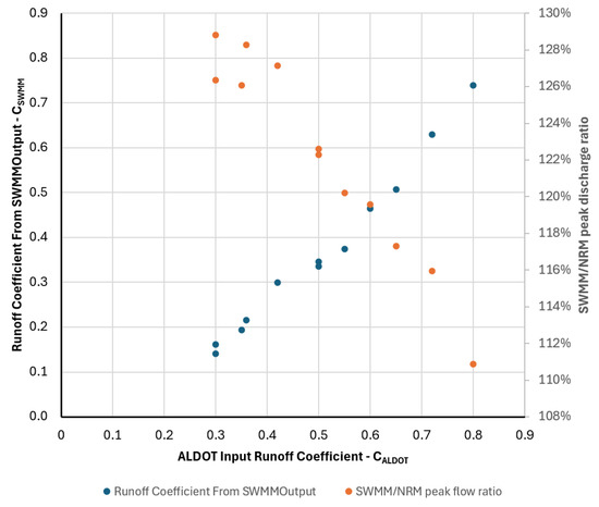
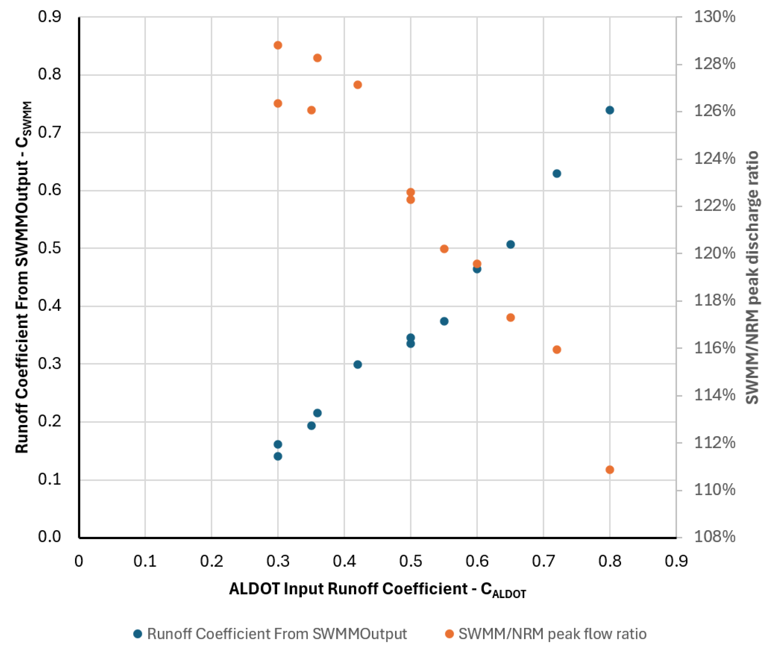
Figure 7 further illustrates a systematic difference between the NRM and SWMM in how each represents rainfall abstraction. The source runoff coefficient from ALDOT ($C_{ALDOT})$ is rate-based and is thus a ratio between the peak runoff discharge and the rainfall intensity, whereas the SWMM’s $C_{SWMM}$ is a volume-based result computed from the model’s mass balance. The observed relationship $C_{SWMM}/C_{ALDOT}$ is approximately linear, with a slope of 1.13. This slope is reflected in the ratios between the SWMM’s peak discharge predictions and NRM peak discharges, as presented in Figure 1.

Figure 7. Assessment 1—runoff coefficient obtained from SWMM Output ($C_{SWMM}$) and ratio between SWMM and NRM peak discharges plotted against the input $C_{ALDOT}$ from ALDOT manual. A linear trendline is included.

This departure from the 1:1 line can be explained by how the SWMM applies the Curve Number model. Pitt’s [29] method expressed in Equation (7) sets the CN so that the target SCS equation returns $C\cdot P$ when evaluated with the storm depth P at the NRM critical rainfall duration. The CN’s runoff-versus-rainfall relationship is nonlinear and integrated over the time course of the storm. While NRM’s abstraction is constant over the duration of the storm, the abstraction created by CN infiltration in the SWMM decays over time, which apparently has a larger effect on conditions of low runoff coefficient values. The largest discrepancies between the SWMM and NRM’s predictions occur for the lowest $C_{ALDOT}$ values, as is shown in Figure 7. As $C_{ALDOT}$ and the corresponding CN values increase, the discrepancy between the peak discharges decreases monotonically to about 11%.

3.2. Assessment 2: Birmingham Soccer Field Case Study

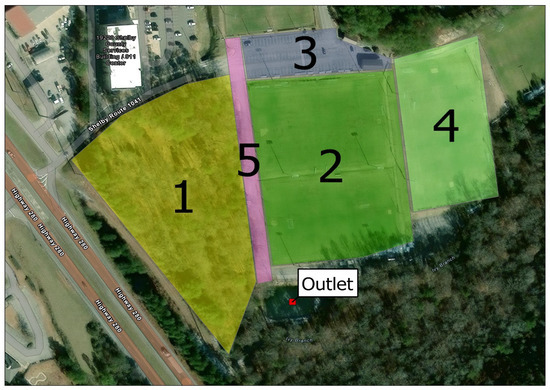
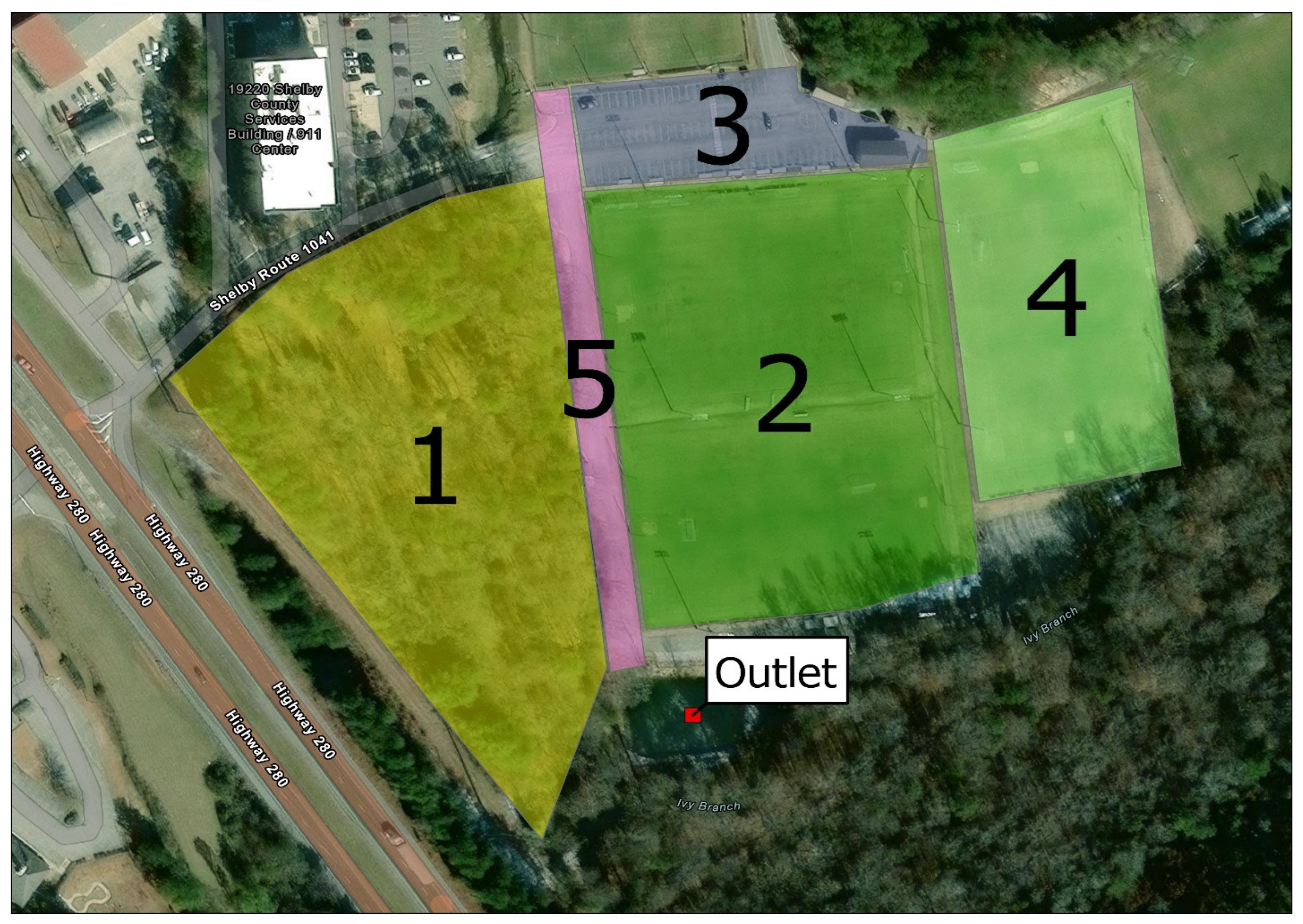
Watershed characteristics for a soccer field and its subareas in Birmingham, Alabama are reported in Table 3, and the corresponding subarea peak-flow results for a soccer field in Birmingham, Alabama, over a 5-year recurrence are reported in Table 4. The layout of the watershed and corresponding subareas is shown in Figure 8. Outflow hydrographs at the outlet were computed under each of the four methods, i.e., NRM, SWMM, PFSA—Velocity, and PFSA—Kerby.

Figure 8. Assessment 2—Birmingham, AL, soccer field watershed with five subareas ro Each subarea is labelled.uted to a common outlet (after Yang [24]). Subcatchments are identified by numbers, with more details provided in Table 3.

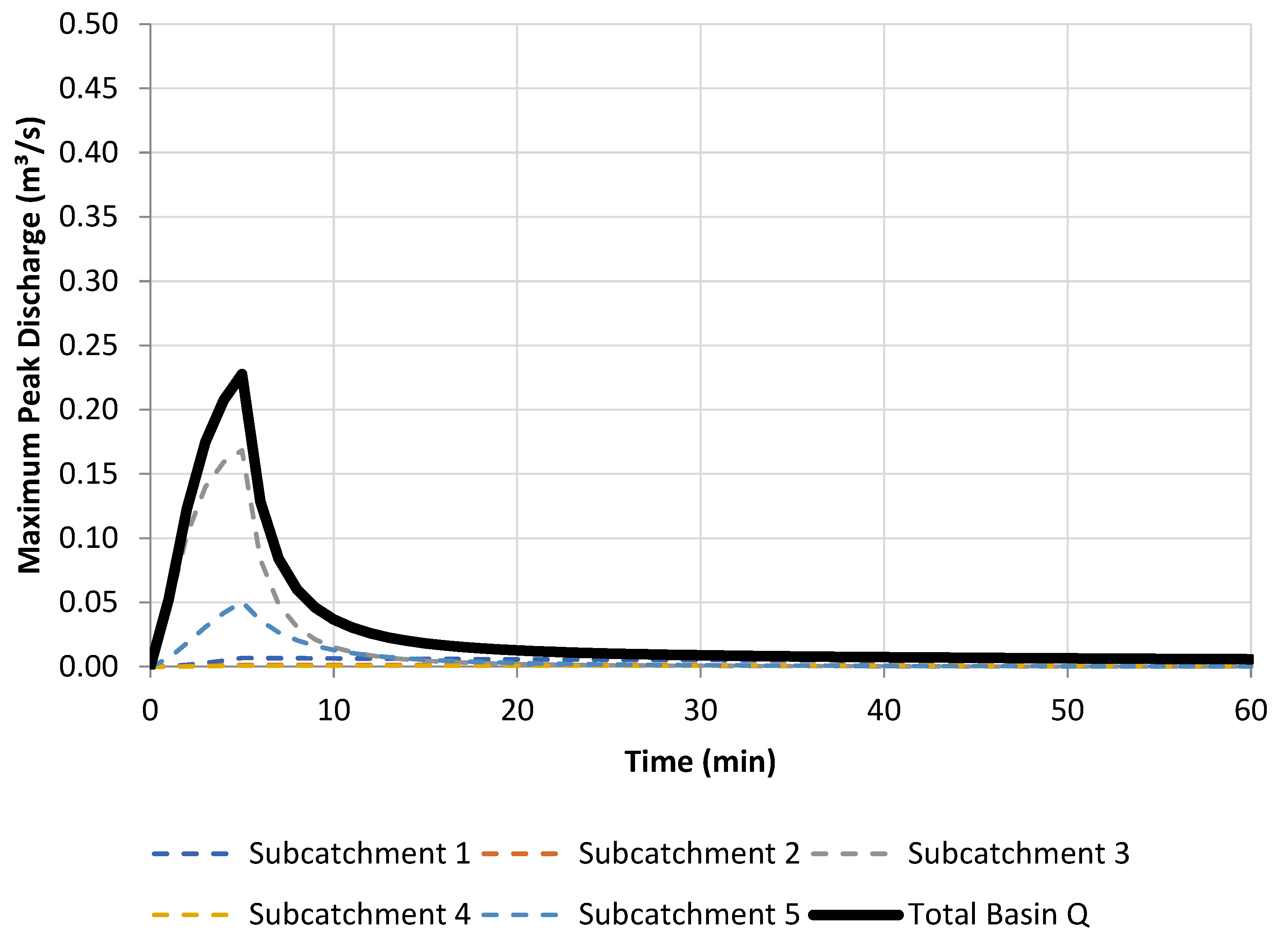
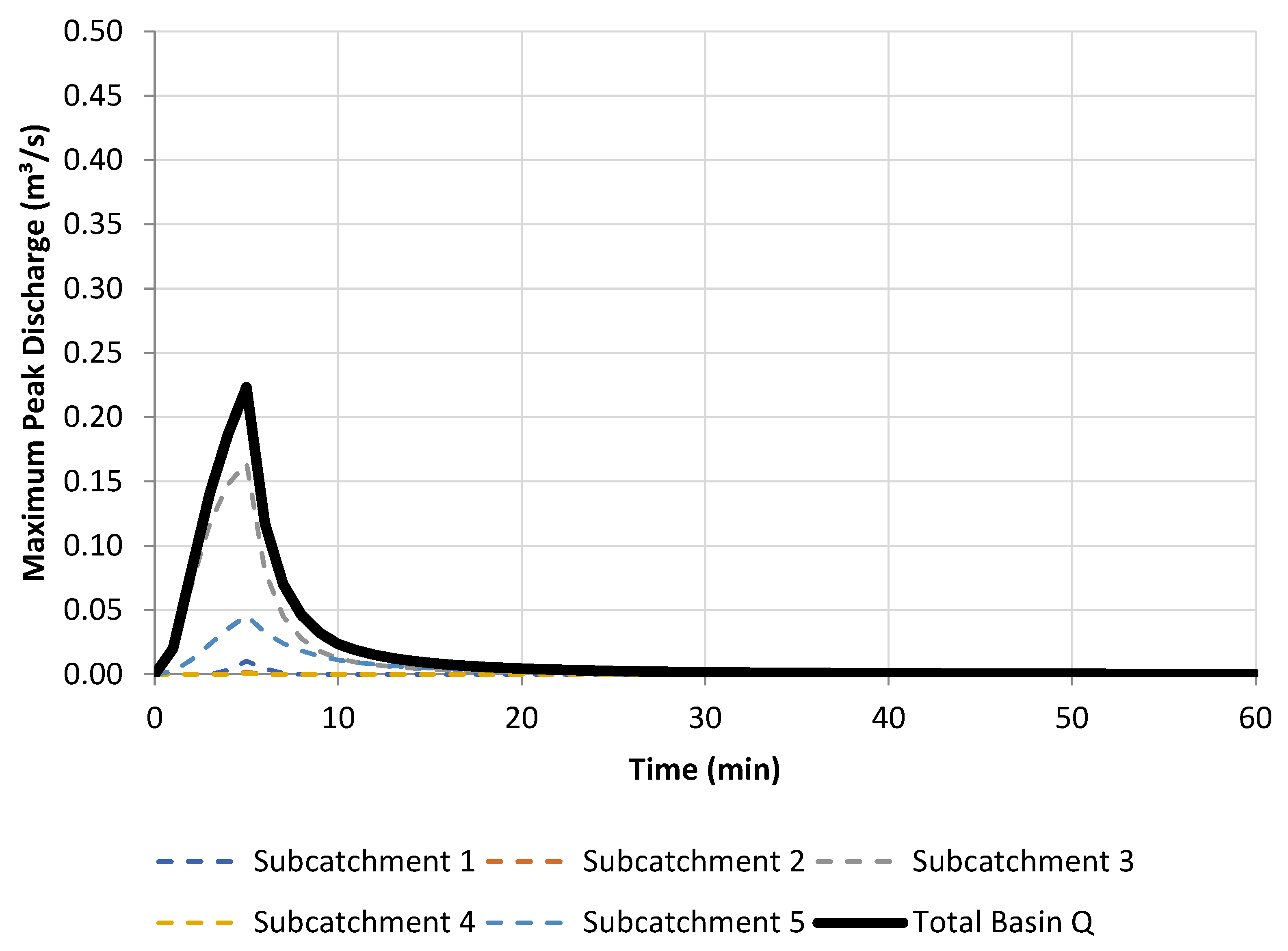
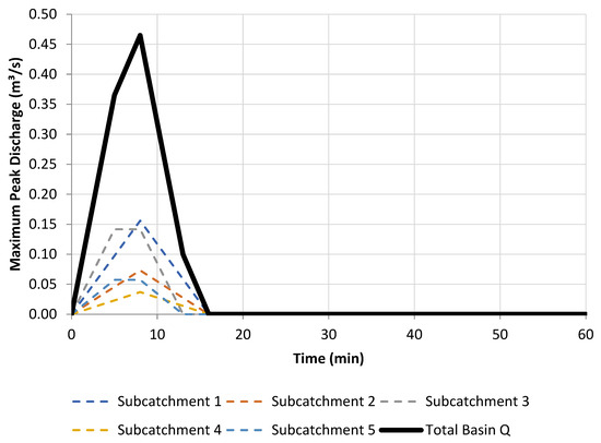
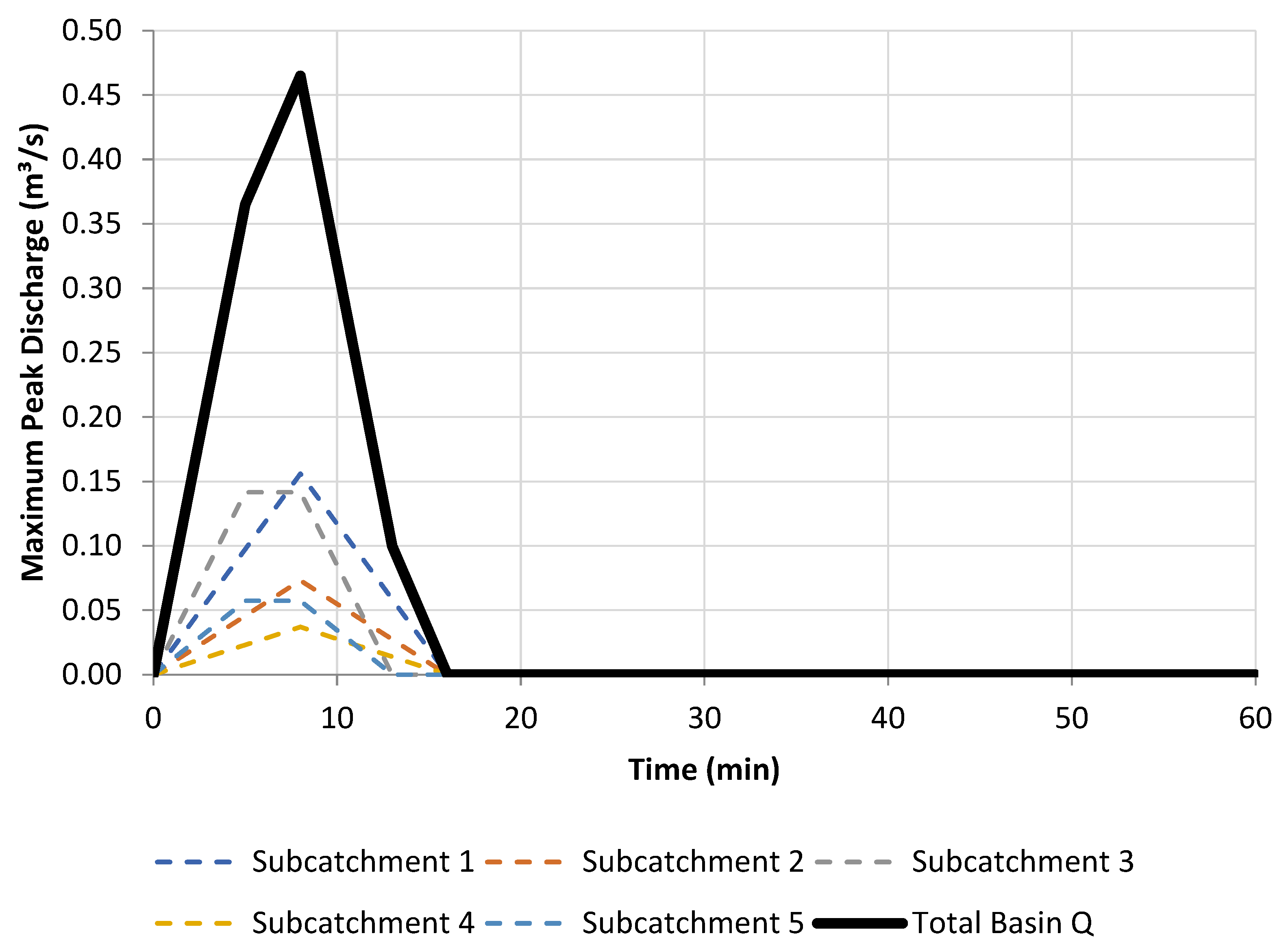
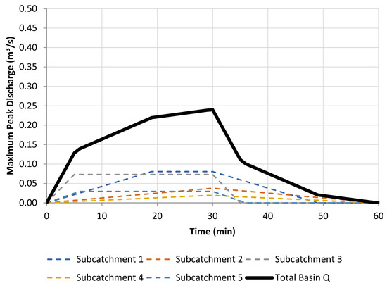
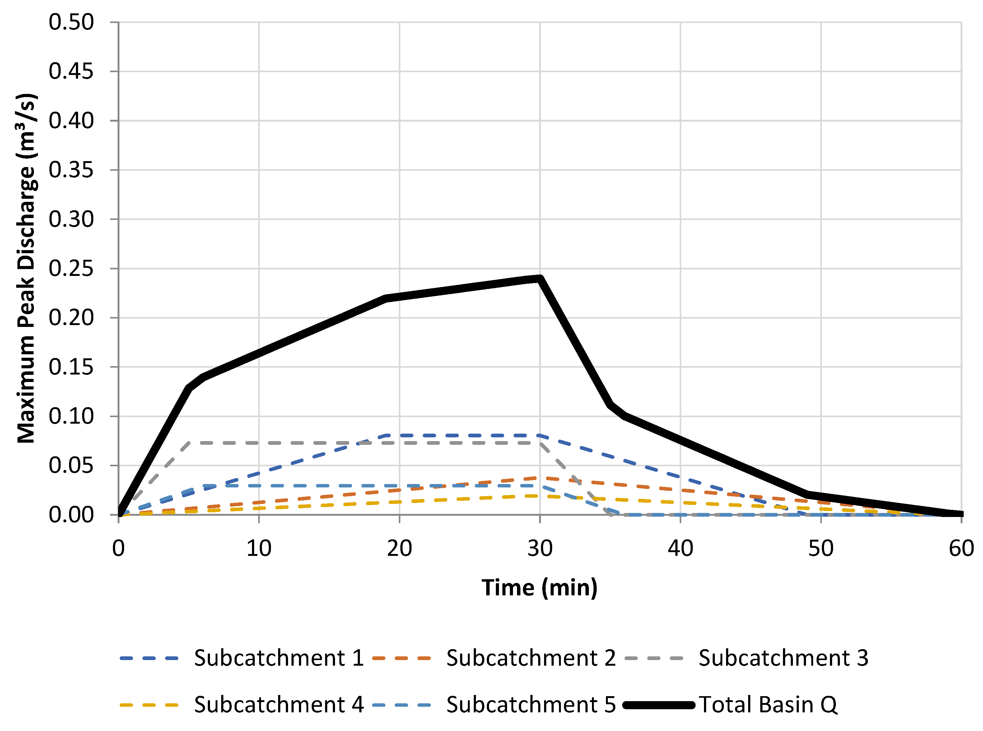
Considering the whole-watershed peak discharges, the NRM and SWMM agreed within 2% (NRM = 0.228 m³/s; SWMM = 0.219 m³/s). The PFSA watershed peak using the Velocity T_c method was substantially larger (0.465 m³/s), corresponding to a Q_PFSA/Q_NRM ratio of 2.0. The Kerby T_c method returned a watershed peak (0.240 m³/s) close to both the NRM and SWMM, highlighting the well-documented sensitivity to the choice of T_c estimation formula in RM-based models, including the PFSA.

Table 3. Assessment 2 input parameters for the Birmingham, AL, soccer field site (after Yang [24]).

Subarea	Area (m2)	Runoff Coefficient	Slope (m/m)	Adopted Manning n	Flow Length (m)
1	21,165	0.18	0.198	0.40	182.3
2	17,847	0.10	0.010	0.15	168.5
3	3602	0.96	0.010	0.011	36.6
4	9024	0.10	0.010	0.15	148.1
5	1457	0.96	0.030	0.011	198.1

Table 3. Assessment 2 input parameters for the Birmingham, AL, soccer field site (after Yang [24]).

Subarea	Area (m2)	Runoff Coefficient	Slope (m/m)	Adopted Manning n	Flow Length (m)
1	21,165	0.18	0.198	0.40	182.3
2	17,847	0.10	0.010	0.15	168.5
3	3602	0.96	0.010	0.011	36.6
4	9024	0.10	0.010	0.15	148.1
5	1457	0.96	0.030	0.011	198.1

Table 4. Assessment 2 watershed-level peak discharge and critical duration results for the Birmingham soccer field site for the 5-year recurrence.

Location	Maximum Peak Discharge Qp (m3/s)				${\mathit{\tau }}_{\mathit{c}\mathit{r}\mathit{i}\mathit{t}}$ for NRM & SWMM or Tc for PFSA (min)
	NRM	SWMM	PFSA Vel.	PFSA Kerby	NRM	SWMM	PFSA Vel.	PFSA Kerby
Whole area	0.228	0.219	0.465	0.240	5	5	8	30
Subarea 1	0.007	0.007	0.156	0.080	60	60	8	19
Subarea 2	0.001	0.001	0.073	0.038	60	59	8	30
Subarea 3	0.168	0.165	0.142	0.073	5	5	5	5
Subarea 4	0.001	0.001	0.037	0.019	60	57	8	29
Subarea 5	0.050	0.046	0.057	0.030	7	8	5	6

Table 4. Assessment 2 watershed-level peak discharge and critical duration results for the Birmingham soccer field site for the 5-year recurrence.

Location	Maximum Peak Discharge Qp (m3/s)				${\mathit{\tau }}_{\mathit{c}\mathit{r}\mathit{i}\mathit{t}}$ for NRM & SWMM or Tc for PFSA (min)
	NRM	SWMM	PFSA Vel.	PFSA Kerby	NRM	SWMM	PFSA Vel.	PFSA Kerby
Whole area	0.228	0.219	0.465	0.240	5	5	8	30
Subarea 1	0.007	0.007	0.156	0.080	60	60	8	19
Subarea 2	0.001	0.001	0.073	0.038	60	59	8	30
Subarea 3	0.168	0.165	0.142	0.073	5	5	5	5
Subarea 4	0.001	0.001	0.037	0.019	60	57	8	29
Subarea 5	0.050	0.046	0.057	0.030	7	8	5	6

Each subarea peak discharge computed by the NRM and SWMM was very similar, as shown in Table 4, with both methods identifying the impervious Subarea 3 as the dominant contributor to runoff peak discharges (NRM = 0.168 m³/s; SWMM = 0.165 m³/s). The pasture subareas (Subareas 2 and 4) and the woodland subarea (Subarea 1) produced very small NRM peaks (0.001–0.007 m³/s). It was found that, if subcatchments 1, 2 and 4 were considered independently, a larger τ (~60 min) would result in larger peak discharges from these areas, though still relatively smaller than the runoff from the areas with the high-C subareas. Subarea PFSA—Velocity peak discharges were much larger than the values for either the NRM or SWMM, while PFSA—Kerby peak discharges were closer to those for the NRM and SWMM across most subareas, exceeding them in the low-C subareas.

Figure 9, Figure 10, Figure 11 and Figure 12 present the watershed outflow hydrographs at the outlet under each of the four methods. NRM and SWMM peak discharges occur at similar times and with similar magnitudes, but the SWMM’s recession limb declines more rapidly than the NRM’s. This difference can be explained by the SWMM’s Curve Number abstraction, presented as infiltration, which continues after the rain event is over [5]. By contrast, the NRM mass balance reverts to pure drainage with no infiltration once the storm ends. Such differences, along with the current inability of the NRM to consider flow routing times, may affect hydrograph calculations and estimates for detention basin volumes when compared to the SWMM. However, considering the greater simplicity of the NRM, the lower data requirement to use the method, and the absence of $T_c$ computation uncertainties, NRM may become an attractive approach to estimate peak runoff discharges and compute hydrographs.

Figure 9. Assessment 2—NRM combined basin hydrograph at the watershed outlet for the 5-year recurrence, aggregated across the five subareas. τ is at 5 min.

Figure 10. Assessment 2—SWMM combined basin hydrograph at the watershed outlet for the 5-year recurrence. τ is at 5 min.

Figure 11. Assessment 2—PFSA combined basin hydrograph at the watershed outlet for the 5-year recurrence using the Velocity T_c method (T_c = 8 min).

Figure 12. Assessment 2—PFSA combined basin hydrograph at the watershed outlet for the 5-year recurrence using the Kerby T_c method (T_c = 30 min).

3.3. Assessment 3: NRM Assessment with Experimental Data

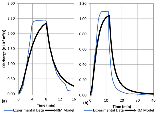
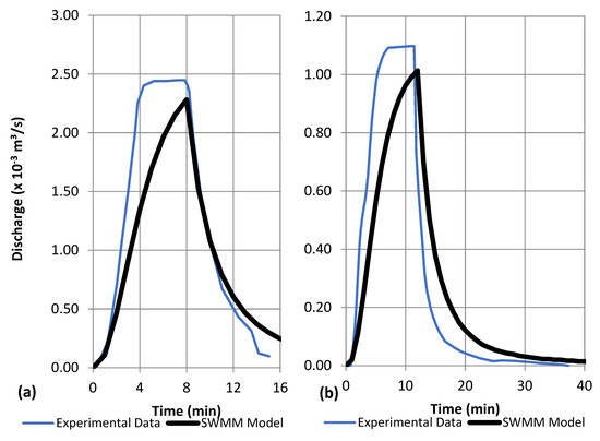
NRM was run with the reported geometry, roughness, and rainfall inputs; the resulting simulated hydrographs at those specific rainfall durations (without searching the critical durations) were compared with the experimental data [25,26] in Figure 13 and Figure 14. The anomalous spike in the measured flow rate in [26], created by the discontinuing of the rainfall during the experiments, was omitted from the experimental hydrograph.

Figure 13. Assessment 3—observed and simulated hydrographs with NRM for (a) concrete surface 152.4 m long and 0.3 m wide with slope of 2%; (b) concrete surface 21.9 m long and 1.8 m wide with slope of 0.1%.

Figure 14. Assessment 3—observed and simulated hydrographs with SWMM for (a) concrete surface 152.4 m long and 0.3 m wide with slope of 2%; (b) concrete surface 21.9 m long and 1.8 m wide with slope of 0.1%.

A comparison between the NRM and the experimental data is presented in Figure 13a,b for Experiments 1 and 2, respectively. The NRM reproduced the observed peak discharge closely in both cases. For Experiment 1, the NRM returns a peak of 2.35 × 10⁻³ m³/s against an observed value of 2.45 × 10⁻³ m³/s (4% difference), whereas for Experiment 2 NRM peak flow was 1.04 × 10⁻³ m³/s against an observed value of 1.10 × 10⁻³ m³/s (5% difference). The integration of these graphs, i.e., the runoff volume, shows a discrepancy of 4.5% for Experiment 1 and 8.3% for Experiment 2 between NRM results and observed models.

It is noticeable that the observed rise in the flow rate is faster in the experimental data, and once the fixed rainfall is over, the predicted NRM drainage is more gradual. This is explained by the lack of spatial discretization in overland flow calculations by the Nonlinear Reservoir Algorithm, which impacts the dynamic flow response in these subcatchments that are channel-shaped [31] performed similar calculations using a discretized numerical model, with results that more closely resemble the measured ones. This indicates that for large length-to-width ratios, a variant of the Saint-Venant equation with lateral inflows could provide more accurate predictions, though it would negate the benefits of using a low-data-requirement approach such as the NRM.

To demonstrate that the differences in hydrograph shape are linked to the use of the Nonlinear Reservoir Algorithm, this same comparison was repeated using the SWMM assuming CN = 99. The results were similar to the ones obtained with the NRM, with peak flows of 2.28 × 10⁻³ m³/s for Experiment 1 and 1.01 × 10⁻³ m³/s for Experiment 2, as shown in Figure 14a,b, respectively. By comparison, SWMM peak flows are slightly smaller than for the NRM, with the recession limb also more gradual than the observed recession. Though no experimental data was available for comparison, it is speculated that applying the NRM to subcatchments with width/length ratios closer to unity would yield hydrographs that are closer to observed hydrographs.

A few summarizing observations from the three assessments presented here are as follows:

•

NRM reproduces the SWMM peak within 15% for most of Assessment 1’s cases, though there is a systematic underprediction ranging from 11% to 29% depending mostly on the runoff coefficient. This discrepancy was much smaller (within 2%) for the entire watershed of Assessment 2. The similarity of NRM peak flows to the SWMM indicates that the proposed method is a viable substitute for RM-based approaches that rely on T_c estimates at least for the range of conditions tested.

•

PFSA peak discharges were overestimated relative to the NRM and SWMM in both Assessment 1 and Assessment 2, though the choice of the $T_c$ computation formula has a major effect on the observed discrepancies. Better comparison was achieved with the PFSA using Kerby $T_c$, and the corresponding $T_c$ computed with the Kerby method was closer to the critical rainfall duration ${\tau }_c$ obtained either by the NRM or SWMM for both Assessment 1 and 2.

•

The discrepancy in the recession limb for Assessment 2 between the NRM and SWMM identifies a limitation of the NRM, as an RM-derived method, in stopping abstractions even if there is water flowing through subcatchments. Unless a time-varying alternative to $C$ is proposed to represent abstractions after the rain event stops, this limitation will remain in the NRM. Yet this limitation does not affect the peak discharge estimation.

•

NRM comparison against experimental hydrographs in Assessment 3 indicates its ability to represent experimental conditions. The assessment also showed the limitations of the NRA, which may affect the shape of hydrographs for linear-shaped subcatchments.

4. Conclusions and Next Steps

This paper proposed the Nonlinear Rational Method or NRM, which retains the low data requirements of the RM for characterizing subcatchment rainfall abstraction while replacing the classical assumption of a single time of concentration with a search over rainfall durations coupled with the SWMM Nonlinear Reservoir Algorithm to route overland flows. The NRM was benchmarked against the SWMM and the PFSA (using the Velocity and Kerby T_c methods) through three assessments: a controlled twelve-case sensitivity study across the ALDOT land-use catalog, a five-subarea watershed application to a soccer field site in Birmingham, Alabama, and a benchmark test against two experimental tests with set rainfall durations.

Across all three assessments, NRM produced peak discharges in close agreement with the SWMM without requiring any T_c formula. The mean SWMM/NRM peak ratio was 1.22 across the twelve Assessment 1 cases, and the NRM matched the SWMM within 2% at the whole-watershed scale of Assessment 2. PFSA solutions overestimated peak discharges by approximately a factor of two relative to the NRM and SWMM under the Velocity T_c method, while the PFSA with the Kerby T_c method returned peak discharges and times to peak closer to the NRM—illustrating the well-documented sensitivity of RM-family methods to the choice of T_c formula, which NRM sidesteps. Assessment 3 compared NRM hydrographs with experimental results, indicating the ability of the method to reproduce the peak flows, though discrepancies in the shape of the hydrographs were noticed.

While NRM brings a key advantage of not considering the time of concentration in the calculations, it also has its own limitations. The method should not be applied in complex or large watersheds in which flow routing effects in hydrographs are relevant, an observation that is also applicable to other RM-based models. Flow path lengths and Manning roughness are key in NRM calculations; thus, such parameters should be carefully evaluated when using the NRM, as is also the case when using the SWMM.

A next step for NRM development is to account for the travel time between subareas so that partial contributions from remote subcatchments can be routed to the watershed outlet with a physically consistent delay. The current NRM implementation, like the RM and its variants, aggregates subcatchment outflows directly without accounting for the time required for flow to reach the outlet from each contributing area. Incorporating a travel-time component would strengthen the NRM’s applicability to larger, multi-subcatchment watersheds where the assumption of instantaneous flow aggregation becomes less adequate and would complement the recession-limb work that will be needed to extend the NRM beyond peak-flow estimation into detention-storage design.

References

- Moore, M.F.; Vasconcelos, J.G.; Zech, W.C. Modeling Highway Stormwater Runoff and Groundwater Table Variations with SWMM and GSSHA. Am. Soc. Civ. Eng. 2017, 22, 04017025. [Google Scholar] [CrossRef] [Scilit]
- Bragg, M.A. Modeling Hydrology and Water Quality in Moore’s Mill Creek Using the Storm Water Management Model (SWMM). Master’s Thesis, Department of Civil and Environmental Engineering, Auburn University, Auburn, AL, USA, 2025. [Google Scholar]
- Poudel, A. Comparative Assessment of HEC-HMS 2D and HEC-RAS 2D Rain-on-Grid for Continuous Urban Watershed Modeling. Master’s Thesis, Department of Civil and Environmental Engineering, Auburn University, Auburn, AL, USA, 2025. [Google Scholar]
- de Oliveira Sousa, B.J.; Morgado, L.M.; Vasconcelos, J.G. Evaluating Distributed Hydrologic Modeling to Assess Coastal Highway Vulnerability to High Water Tables. Water 2025, 17, 2327. [Google Scholar] [CrossRef] [Scilit]
- Rossman, L.A.; Huber, W.C. Storm Water Management Model Reference Manual, Volume I—Hydrology (Revised); EPA/600/R-15/162A; U.S. Environmental Protection Agency: Cincinnati, OH, USA, 2016. Available online: https://www.epa.gov/water-research/storm-water-management-model-swmm (accessed on 15 August 2026).
- National Academies of Sciences, Engineering, and Medicine. Resilient Design with Distributed Rainfall-Runoff Modeling; The National Academies Press: Washington, DC, USA, 2023. [Google Scholar] [CrossRef] [Scilit]
- Alabama Department of Transportation (ALDOT). Hydrology Manual; ALDOT: Montgomery, AL, USA, 2018.
- Chin, D.A. Estimating peak runoff rates using the rational method. J. Irrig. Drain. Eng. 2019, 145, 04019006. [Google Scholar] [CrossRef] [Scilit]
- Mulvaney, T.J. On the use of self-registering rain and flood gauges in making observations of the relations of rainfall and flood discharges in a given catchment. Proc. Inst. Civ. Eng. Irel. 1851, 4, 18–33. [Google Scholar]
- Kuichling, E. The relation between the rainfall and the discharge of sewers in populous districts. Trans. Am. Soc. Civ. Eng. 1889, 20, 1–56. [Google Scholar] [CrossRef] [Scilit]
- Wright-McLaughlin Engineers. Urban Storm Drainage Criteria Manual; Denver Regional Council of Governments and the Urban Drainage and Flood Control District: Denver, CO, USA, 1969.
- Guo, J.C.Y.; Urbonas, B. Volume-based runoff coefficients for urban catchments. J. Irrig. Drain. Eng. 2013, 140, 04013004. [Google Scholar] [CrossRef] [Scilit]
- Dhakal, N.; Fang, X.; Cleveland, T.G.; Thompson, D.B.; Asquith, W.H.; Marzen, L.J. Estimation of volumetric runoff coefficients for Texas watersheds using land-use and rainfall-runoff data. J. Irrig. Drain. Eng. 2012, 138, 43–54. [Google Scholar] [CrossRef] [Scilit]
- Froehlich, D.C. Return period–dependent rational formula coefficients for two locations in Texas. J. Irrig. Drain. Eng. 2016, 142, 04016035. [Google Scholar] [CrossRef] [Scilit]
- Poertner, H.G. Practices in Detention of Urban Stormwater Runoff: An Investigation of Concepts, Techniques, Applications, Costs, Problems, Legislation, Legal Aspects and Opinions; American Public Works Association: Chicago, IL, USA, 1974. [Google Scholar]
- Smith, A.A.; Lee, K.-B. The rational method revisited. Can. J. Civ. Eng. 1984, 11, 854–862. [Google Scholar] [CrossRef] [Scilit]
- Vasconcelos, J.G.; Gomes, M.N., Jr.; Oliveira, P.T.S.; Yang, D.; Fang, X. Reformulating the rational method considering dissimilar land use types. J. Irrig. Drain. Eng. 2025, 151, 04025017. [Google Scholar] [CrossRef] [Scilit]
- Grimaldi, S.; Petroselli, A.; Tauro, F.; Porfiri, M. Time of concentration: A paradox in modern hydrology. Hydrol. Sci. J. 2012, 57, 217–228. [Google Scholar] [CrossRef] [Scilit]
- Fang, X.; Thompson, D.B.; Cleveland, T.G.; Pradhan, P.; Malla, R. Time of concentration estimated using watershed parameters determined by automated and manual methods. J. Irrig. Drain. Eng. 2008, 134, 202–211. [Google Scholar] [CrossRef] [Scilit]
- McCuen, R.H. Uncertainty analyses of watershed time parameters. J. Hydrol. Eng. 2009, 14, 490–498. [Google Scholar] [CrossRef] [Scilit]
- Gericke, O.J.; Smithers, J.C. Review of methods used to estimate catchment response time for the purpose of peak discharge estimation. Hydrol. Sci. J. 2014, 59, 1935–1971. [Google Scholar] [CrossRef] [Scilit]
- Simpson, I.M.; Yoder, D.C.; Hathaway, J.M. Simple solutions for improving urban peak flow estimates at the watershed scale. J. Hydrol. Eng. 2026, 31, 05026009. [Google Scholar] [CrossRef] [Scilit]
- Press, W.H.; Teukolsky, S.A.; Vetterling, W.T.; Flannery, B.P. Numerical Recipes in C: The Art of Scientific Computing, 2nd ed.; Cambridge University Press: Cambridge, UK, 1992. [Google Scholar]
- Yang, D. Application of the Peak Flow Search Approach to Dissimilar-Land-Use Catchments in Central Alabama. Master’s Thesis, Department of Civil and Environmental Engineering, Auburn University, Auburn, AL, USA, 2024. [Google Scholar]
- Yu, Y.S.; McNown, J.S. Runoff from impervious surfaces. J. Hydraul. Res. 1964, 2, 3–24. [Google Scholar] [CrossRef] [Scilit]
- Izzard, C.F.; Augustine, M.T. Preliminary report on analysis of runoff resulting from simulated rainfall on a paved plot. Eos Trans. Am. Geophys. Union 1943, 24, 500–509. [Google Scholar] [CrossRef] [Scilit]
- Natural Resources Conservation Service (NRCS). Time of concentration. In National Engineering Handbook: Part 630—Hydrology; 210-VI-NEH; Chapter 15; U.S. Department of Agriculture: Washington, DC, USA, 2010. Available online: https://directives.sc.egov.usda.gov/ (accessed on 15 August 2026).
- Texas Department of Transportation (TxDOT). Hydraulic Design Manual, 5th ed.; TxDOT: Austin, TX, USA, 2019. Available online: https://www.txdot.gov/manuals/des/hyd/index.html (accessed on 15 August 2026).
- Pitt, R. Small storm hydrology and why it is important for the design of stormwater control practices. In Advances in Modeling the Management of Stormwater Impacts; James, W., Ed.; CHI Publications: Guelph, ON, Canada, 1999; Volume 7. [Google Scholar]
- Soil Conservation Service (SCS). Urban Hydrology for Small Watersheds, Technical Release 55 (TR-55), 2nd ed.; U.S. Department of Agriculture: Washington, DC, USA, 1986.
- KC, M.; Fang, X.; Yi, Y.-J.; Li, M.-H.; Thompson, D.B.; Cleveland, T.G. Improved Time of Concentration Estimation on Overland Flow Surfaces Including Low-Sloped Planes. J. Hydrol. Eng. 2013, 19, 495–508. [Google Scholar] [CrossRef] [Scilit]
Disclaimer/Publisher’s Note: The statements, opinions and data contained in all publications are solely those of the individual author(s) and contributor(s) and not of MDPI and/or the editor(s). MDPI and/or the editor(s) disclaim responsibility for any injury to people or property resulting from any ideas, methods, instructions or products referred to in the content. |
© 2026 by the authors. Licensee MDPI, Basel, Switzerland. This article is an open access article distributed under the terms and conditions of the Creative Commons Attribution (CC BY) license.