Predictive Maintenance in Logistics Fleets: A Comparative Evaluation of Random Forest, XGBoost, and Logistic Regression Using Operational and Technical Indicators

Abstract

Background: Predictive maintenance (PdM) is increasingly recognized as essential for reducing fleet downtime and maintenance costs, yet the existing literature on transport and logistics fleets relies predominantly on traditional or single-model approaches, with ensemble methods such as random forest and gradient boosting remaining comparatively underexplored. Methods: This study develops and compares three classification algorithms—logistic regression, random forest and XGBoost—for predicting vehicle maintenance needs. Each classifier was first fitted once on a 70:30 train–test split (35,000/15,000 observations) to support interpretation of coefficients, predictor importance, and ROC curves, using precision, recall, and ROC-AUC. Performance and model ranking were then confirmed for robustness using 5-fold stratified cross-validation with formal significance testing. Results: Reported issues and service history emerged as the dominant predictors of maintenance needs. Random forest and XGBoost achieved comparable predictive performance under 5-fold cross-validation (mean AUC-ROC of 0.8546 and 0.8528, respectively), with the difference between them not statistically significant; both clearly outperformed logistic regression (AUC-ROC 0.8215). Conclusions: By integrating operational and technical data within a validated, comparative machine learning framework, the study provides a practical basis for decision-support systems enabling the reduction of unnecessary interventions, minimizing downtime, and improving fleet cost efficiency and reliability.

1. Introduction

The rapid acceleration of technological evolution in the modern era has fundamentally redefined industrial paradigms, imposing unprecedented demands on operational efficiency and precision. At the heart of this shift lies Industry 4.0, a framework characterized by the integration of Cyber–Physical Systems (CPS), the Internet of Things (IoT), and advanced data analytics [1].

A critical implication of this digital transformation is the strategic transition from reactive maintenance—addressing equipment failure after it occurs—to predictive maintenance. By leveraging real-time sensor data and machine learning algorithms, organizations can now anticipate technical anomalies, thereby optimizing lifecycle management and minimizing systemic downtime.

Fleet downtime acts as a systemic bottleneck where mechanical failures trigger a domino effect of ‘hidden’ logistical costs—ranging from shattered delivery windows to unproductive driver idle time—that ultimately destabilizes the efficiency and reliability of the global trade network and it can be determined mainly by parts shortages, delays and the complexity of repairs.

1.1. Cost Implications of Maintenance Activities

According to a report from 2025 [2], parts and maintenance delays cause a drastic reduction in shipments, generating pressure on the management. It is estimated that in the automotive industry, the downtime cost per vehicle ranges between $448 and $760 a day, mostly due to part malfunctions leading to fleet breakdowns [3], and reaching values up to $1000 per day when both repair costs and lost productivity are encompassed [4,5]. For the entire automotive industry, in terms of plant downtime, the costs reach high levels of more than $2,000,000 per hour.

According to [6], the costs of products include, among the main manufacturing aspects, inefficiencies, poor performance, avoidable mistakes, but also repairs and reworks, the latter summing up to more than 15% of the costs of any products or equipment.

A reduction in repair-related costs can be achieved through the transition from reactive (to act when the failure occurs) to preventive (scheduled activities) and furthermore, predictive maintenance strategies (to forecast the need for maintenance). In recent years, this transition has emerged as a paradigm shift in maintenance practices within the automotive sector, reflecting a systematic move toward data-driven and condition-based approaches. The importance of adopting predictive activities lies in its capacity to reduce maintenance-related expenses, as suggested by field guides available online [7,8] which revealed a reduction in costs by up to 25–30% compared to applying reactive maintenance.

In Europe only, it is presumed that more than 60% of large logistic companies use predictive maintenance as a strategy, leading to an increase in fleet uptime by 50% and a maintenance cost reduction of 40% [9].

In essence, as defined by the European standard [10], predictive maintenance is performed through the implementation of a set of actions based on prognostic assessments, derived from repeated analyses or from components known to be failure-prone or whose operational parameters exhibit measurable degradation over time. As opposed to reactive or preventive maintenance, the predictive approach involves continuous condition monitoring of equipment via sensors and the use of real-time data. This involves a shift in the distribution of costs on the entire life cycle of a product, with emphasis on upfront investments on monitoring tools, but with lower costs in the long term. In addition to the cost advantage, predictive maintenance also implies avoiding unnecessary work, reduced unplanned downtime and extension of product life [11,12].

1.2. State-of-the-Art Review of Failure Prediction Techniques and Diagnostic Approaches

Given the growing importance of predictive maintenance in modern industrial systems, it is necessary to examine the current methodologies employed for failure prediction and equipment diagnostics. Recent studies regarding the application of predictive maintenance focused on three main directions: sensor-based condition monitoring techniques, data-driven failure prediction models (such as machine learning models, deep learning approaches: convolution or recurrent neural networks and pattern recognition and anomaly detection) and model-based and physics-based diagnostic approaches (such as reliability and degradation models). In addition, the newest analysis techniques have a hybrid approach, involving the integration of AI into traditional means.

In terms of sensor–based condition monitoring, as a strategy for condition-based maintenance (CBM), data acquisition and processing are the main parts of the investigative activity [13,14]. Scientific articles such as [15] present key methodologies and signal processing tools (e.g., wavelets, Fast Fourier Transform (FFT), and Complete Ensemble Empirical Mode Decomposition with Adaptive Noise (CEEMDAN)) as a fundamental component of condition monitoring systems, emphasizing their role in extracting informative features from sensor signals to enable reliable fault detection and enhance predictive maintenance capabilities.

Other papers [16] propose the use of innovative methods such as IoT for collecting and managing real-time data provided by sensors, as the processes generate complex datasets. The novel approach for fault detection and Remaining Useful Life (RUL) prediction consists of the use of Autoencoders with Long Short-Term Memory (LSTM) networks for processing multivariate data, detecting anomalies and filtering the data.

A comprehensive study from 2025 [17] focused on maintenance practices in the manufacturing sector, performed based on patent data rather than scientific publications, and highlighted a correlation between the terms predictive maintenance and machine learning, among others, suggesting that the use of the latter is becoming more relevant in the context of predictive maintenance. According to the authors, the use of predictive maintenance, as opposed to traditional strategies, leads to a substantial reduction in costs and an increase in operational uptime when AI (artificial intelligence) and IoT (Internet of Things) are used.

At a larger scale, in the logistic fleet management, there are studies, such as those conducted by [18] which present a stochastic optimization framework to improve fleet readiness through predictive maintenance and mission assignment. It introduces a Fleet Selective Maintenance (FSM) model that determines which systems to maintain, maintenance levels, and mission allocations under uncertainty. The approach combines analytical reliability models with deep neural networks for sensor-monitored components. Uncertainty is handled using chance-constrained optimization, Sample Average Approximation (SAA) and Conditional Value-at-Risk (CVaR) methods.

In the management of transportation companies, studies such as [19] suggest adopting multi-layer conceptual models based on artificial intelligence in order to efficiently process information from fleet, warehouse and enterprise systems so that maintenance, routing and risk management are better performed. The paper describes the phases of data collection, AI analytics, decision support and operational execution in the case of large-volume data, in order to obtain coordinated managerial and operational improvements.

Including high end analysis methods based on Industry 4.0 technologies such as IoT, machine learning, and cloud computing is also the aim of study [20], where the authors propose an integrated predictive maintenance system for reverse supply chain operations. It addresses the challenge of managing dispersed equipment and maintenance activities by enabling real-time data collection and failure prediction. As it is suggested by the authors, the system optimizes maintenance scheduling, spare parts management, and coordination among stakeholders. As a result, it improves efficiency, reduces costs, and extends equipment life cycles within the reverse supply chain.

The use of machine learning techniques to demonstrate maintenance scheduling optimization and improve operational efficiency is also the topic of paper [21], where the use of random forest and decision tree has led to improved prediction accuracy of vehicle maintenance needs.

In terms of fleet management, different challenges may arise due to a series of uncertainties that can affect operational planning and maintenance decisions. To that end, study [21] proposes a hybrid framework that integrates data-driven reliability models, based on deep neural networks, with analytical approaches to predict component failures, within a chance-constrained optimization model for maintenance and mission assignment. By explicitly considering uncertainty and real-time condition monitoring, the approach enhances fleet readiness, optimizes resource allocation, and improves operational efficiency. The framework addresses limitations of conventional methods that treat maintenance planning and mission scheduling independently.

The use of combined analysis techniques such as Long Short-Term Memory (LSTM) neural networks, One-Class (Support Vector) SVM, XGBoost, and statistical methods is useful in a wide range of industries, as proven by the authors in paper [22]. According to the article, the proposed approach of using machine learning for predictive maintenance was useful for anomaly detection in time-series sensor data, as well as for identifying early signs of engine component failures, particularly crosshead bearing defects. The study also developed an ensemble model that improved detection performance by integrating the outputs of individual models.

A particular approach in demonstrating the use of deep learning architectures such as LTSM or machine learning algorithms such as XGBoost for predictive maintenance of mechanical parts was detailed in paper [23] where the results indicate a lowering of Mean Absolute Errors by 9.8% on a subset and by 7.4% on the more challenging one than the values obtained with the use of baseline architectures. These findings demonstrate that advanced ensemble methods significantly enhance early fault detection and support more efficient maintenance planning.

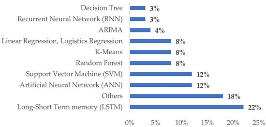
To summarize, article [24] presents a systematic literature review regarding predictive maintenance (PdM) in the transportation sector, reflecting the distribution of methods and algorithms used for estimations.

The available literature on predictive maintenance of transport fleets confirms the growing importance of data-driven maintenance planning. However, the research to date remains methodologically heterogeneous and is only comparable to a limited extent. It should be noted that the existing studies differ significantly in terms of their analytical objective, the type of data used, the structure of variables and the modeling strategies adopted, which makes it difficult to identify which approaches are most useful from the perspective of practical decisions regarding fleet-level maintenance. Therefore, a tabular comparison of previous studies is presented below, discussing the type of method used, the nature of the analyzed datasets, the scope of the variables considered, and the key limitations of each approach.

The comparison presented in Table 1 shows that previous studies differ not only in terms of modeling techniques, but also in the character of their data, analytical objectives, and practical applicability. As can also be seen from Figure 1, it should be noted that random forest models and logistic regression remain relatively rarely used in research on PdM in transport. Furthermore, a research gap has been identified stemming from the fact that most of the currently available studies (e.g., [25]) primarily use sensors as a source of information, thereby requiring advanced IoT infrastructure, which poses a significant practical limitation for small and medium-sized enterprises. In this context, this article is particularly significant as it seeks to address this gap. Firstly, this article demonstrates that predictive maintenance constitutes a significant challenge in the decision-making process regarding transport fleet management and is therefore a more complex issue than a mere classification problem. Secondly, the article proposes an approach, not previously reported in the literature, which enables a comparison of three different models—namely, logistic regression, random forest and the XGBoost model—built on an identical dataset and using the same validation criteria. Thirdly, the study identifies the operational and technical variables that have the greatest influence on classifying data observations as requiring maintenance, which may form the basis for developing maintenance strategies for the transport fleet.

Table 1. Summary of the literature review.

Study	Main Approach	Dataset Type	Main Variables	Key Limitations
Ali and Abdelhadi [13]	State-of-the-art review of condition-based monitoring	Review paper	Sensor monitoring, diagnostics, CBM concepts	Conceptual synthesis; no comparative empirical validation; no fleet-level decision model.
Garcia et al. [15]	Review of signal processing, hybrid models, and implementation challenges	Review-based evidence from industrial equipment studies	Signal processing tools, feature extraction, implementation issues	Broad industrial perspective; no dedicated logistics fleet dataset; limited direct comparison of operational decision usefulness.
Bampoula et al. [16]	LSTM-autoencoders and transformer encoders	Multivariate sensor data from manufacturing assets	Anomaly detection, Remaining Useful Life, filtered multivariate signals	Strong emphasis on sensor-rich environments; limited applicability where only operational and maintenance records are available; not fleet-oriented.
Benhanifia et al. [17]	Systematic review of predictive maintenance practices	Patent-based review in manufacturing	Predictive maintenance, AI, IoT, innovation trends	Patent perspective rather than direct performance comparison; not specific to transport fleets; no common predictive benchmark.
O’Neil et al. [18,22]	Stochastic optimization, reliability models, deep learning, chance-constrained methods	Sensor-monitored systems under uncertainty	Fleet readiness, mission assignment, maintenance allocation	High methodological complexity; focus on mission allocation and optimization under uncertainty rather than straightforward maintenance classification; reduced interpretability for routine fleet decisions
Ando et al. [19]	Multi-layer AI conceptual framework for transportation companies	Conceptual/organizational integration across fleet, warehouse, enterprise systems	AI analytics, decision support, routing, risk management	Architecture-oriented; lacks model-level validation on a common maintenance dataset; no direct classifier comparison.
Gayialis et al. [20]	Integrated predictive maintenance system for reverse supply chain	Real-time data collection and coordination framework	Scheduling, spare parts, stakeholder coordination, failure prediction	System-level orientation; limited focus on transparent comparison of classification models for maintenance qualification.
Mahiyudin et al. [21]	Random Forest and Decision Tree	Vehicle maintenance prediction dataset	Vehicle maintenance need prediction	Narrower comparative scope; no explicit comparison with XGBoost and Logistic Regression under one framework; limited evidence on interpretability-versus-performance trade-off.
Makridis et al. [22]	LSTM, One-Class SVM, XGBoost, statistical methods, ensemble approach	Time-series sensor data in maritime applications	Anomaly detection, early engine failure symptoms	Maritime rather than road logistics setting; focus on time-series anomaly detection; limited transferability to structured fleet-service records.
Ahmed [23]	LSTM and attention-based LSTM-XGBoost hybrid models	Turbofan engine Remaining Useful Life datasets	RUL prediction, deep learning, error reduction	Specialized mechanical domain; emphasis on RUL rather than binary maintenance decision; likely dependence on advanced sequential sensor data.
Ersöz et al. [24]	Systematic literature review in transportation PdM	Review of transportation PdM methods	Distribution of methods and algorithms	Review identifies trends but does not provide empirical head-to-head testing of selected algorithms on one comparable fleet dataset.

Figure 1. Types of methods and algorithms used for PdM estimation [24].

In light of the results presented, the main research problem addressed in this article is to design and empirically validate an approach to predictive maintenance for transport fleets that relies exclusively on operational and technical data routinely recorded in transport management systems, without using advanced sensor infrastructure. In particular, the study examines whether, and to what extent, three widely used classification algorithms—logistic regression, random forest and XGBoost—can reliably and transparently identify vehicles that should be qualified for maintenance, taking into account the constraints of real-world fleet data. This problem is important both scientifically and practically. Despite the dynamic development of sensor-based and deep-learning methods, many transport and logistics operators do not have the resources or data quality required to implement complex CBM solutions. Under such conditions, there is a need for predictive models that are robust, interpretable and based on data already available in typical fleet management systems.

The need for condition-based maintenance (CBM) in transport fleets is usually justified by the requirement to reduce overall operating and maintenance costs while improving vehicle availability and safety. In this context, the present study demonstrates that data-driven predictive models built on routinely collected operational and technical records can support a shift from purely time- or mileage-based schedules towards risk-based planning of maintenance interventions. By linking model outputs to variables such as reported issues, service history and fuel efficiency, the analysis provides a practically interpretable basis for deciding which vehicles should be prioritized for maintenance, thereby reducing unnecessary interventions, minimizing unplanned downtime and improving fleet cost efficiency and reliability.

2. Materials and Methods

In the following article, a vehicle maintenance database was analyzed to build predictive models for assessing the need for maintenance, based on available operational and technical data. The empirical analysis in this study is based on a vehicle maintenance dataset comprising 50,000 records obtained from the transport management system (FireTMS from Poland, produced by Inelo), a multi-service transport-and-logistics operator, whose activity combines core road haulage operations with elements of passenger transport services and an internal service (auxiliary) fleet supporting day-to-day operations. Each record corresponds to an individual vehicle and includes technical specifications (engine size, fuel type, transmission type, vehicle category), operational indicators (mileage, vehicle age, intensity of use, fuel efficiency, time since last service) and maintenance-related information (service history, accident history, maintenance history categories, reported issues and tire condition). These variables were extracted directly from the company’s TMS and reflect the type of data routinely stored in fleet management and maintenance modules of transport and logistics enterprises. This diversified operational profile is reflected in the composition of the “vehicle model” variable presented in Table 2 (SUV, motorcycle, bus, van, truck and car), which spans both freight-oriented vehicles and passenger- and service-oriented units rather than a single homogeneous vehicle class. The records span several consecutive years of operation. For confidentiality reasons, the exact size and detailed organizational structure of the fleet cannot be disclosed. The mixed composition described above is representative of the range of vehicle types typically operated by a multi-service transport-logistics enterprise.

Table 2. Characteristics of the dependent and independent variables used for modeling.

Variable	Type	Scale/Coding Mode
Mileage	Quantitative	Continuous/Discrete
Reported issues	Quantitative	Continuous/discrete
Vehicle age	Quantitative	Continuous/discrete
Engine size	Quantitative	Continuous/discrete
From last service	Quantitative	Continuous/discrete
Service history	Quantitative	Continuous/discrete
Accident history	Quantitative	Continuous/discrete
Fuel efficiency	Quantitative	Continuous/discrete
Intensity	Quantitative	Continuous/discrete
Vehicle model	Qualitative	Nominal, 6 categories: SUV, Motorcycle, Bus, Van, Truck, Car
Maintenance history	Qualitative	Nominal, 3 categories: good, average, poor
Fuel type	Qualitative	Nominal, 3 categories: petrol, diesel, electric,
Transmission type	Qualitative	Nominal, 2 categories: automatic, manual
Owner type	Qualitative	Nominal, 3 categories: first, second, third
Tire condition	Qualitative	Nominal, 3 categories: worn out, new, good
Need maintenance	Binary (dependent)	0 = no service required, 1 = service required

The analytical strategy adopted in this study proceeds in two complementary stages. In the first stage, each of the three classification models is fitted once, following a single 70:30 split of the dataset into training and test sets, enabling direct interpretation of estimated coefficients, predictor-importance rankings, and ROC curves, and yielding an initial, single-split performance comparison. In the second stage, the same three models were rebuilt using the same leakage-safe pipeline, this time embedded within a 5-fold cross-validation procedure, followed by significance testing (Friedman and Wilcoxon tests) and an operational cost analysis. These results are reported later in Section 3 (Tables 12–14). The two stages thus serve different purposes: the single-split analysis supports model interpretation, while the cross-validated analysis supports robust, statistically grounded model comparison and practical decision-making for fleet management.

In this study, the binary outcome “need maintenance” (coded as 0 = no service required, 1 = service required) is used to classify whether a vehicle’s current operational and technical condition qualifies it for a maintenance intervention. The label was constructed based on maintenance records and expert rules applied in the company’s transport management system, combining information such as reported issues, service and accident history, and time since last service into a single qualification rule. Rather than representing a forecast of a future failure event at a specific point in time, the label reflects a cross-sectional assessment of the vehicle’s condition: both the label and all predictor variables were derived from the same observation snapshot, recorded at a single point in the vehicle’s operational history. This precludes the use of information generated after the qualification decision (e.g., a fault occurring or a service being carried out afterward) as a predictor, since no such post-decision information was entered into the feature set. Consequently, all predictors listed in Table 2 were available prior to, or at the same time as, the qualification decision, and none of them encode outcomes that occurred after the label was assigned. Before model development, the dataset was subjected to a systematic data-cleaning procedure: records with missing or inconsistent values in key fields were checked (no records were removed), quantitative variables were checked for outliers using the three-sigma rule, and categorical variables were recoded into coherent category sets as presented in Table 2. The resulting analytical dataset thus represents a consistent and realistic description of fleet operation and maintenance, which is essential for ensuring the credibility, reproducibility and generalizability of the machine learning results reported in this study. For the purpose of this article, fifteen variables (quantitative and qualitative) were selected as independent variables.

Three mathematical models, designed for modeling classification problems (for binary dependent variables), were used to assess the need to send a vehicle for maintenance based on available technical and operational parameters.

The first model was a logistic regression model. Logistic regression is a model that allows the influence of several variables $X_1,X_2,\dots ,X_k$ on the dichotomous variable Y in the mathematical form to be presented. The logistic regression model is based on a logistical function that takes the following form [26]:

$$f\left(x\right)={\displaystyle \frac{e^x}{1+e^x}}={\displaystyle \frac{1}{1+e^{-x}}},$$

(1)

where e is the Euler number, and x is the value of the explanatory variable X.

The use of logistic regression is supported by the fact that it is not required to meet many assumptions that are formulated in relation to linear regression and general linear models. These include, first of all, the linearity of the relationship between a dependent and an independent variable, as well as the normality and homoscedasticity of the distribution of independent variables. In addition, observations must be reported using metric measurement systems.

The logistic regression model can be written in several ways. Assuming that Y stands for a dichotomous variable with values 1 for the occurrence of the event we are interested in (success) and 0 for the opposite case (failure), the logistic regression model is described by Equation (2) [27]:

$$P(Y=1|x_1,x_2,\dots ,x_k)={\displaystyle \frac{e^{{\beta }_0+{\beta }_i·x_i}}{1+e^{{\beta }_0+{\displaystyle {\sum }_{i=1}^k}{\beta }_i·x_i}}},$$

(2)

where ${\beta }_i$ i = 0, …, k are logistic regression factors, while $x_1,x_2,\dots ,x_k$ are independent variables, which can be measurable or qualitative.

An equivalent form of the logistic regression equation can be written as the odds for the occurrence of the event (success) we are interested in:

$${\displaystyle \frac{P(Y=1|X)}{1-P(Y=1|x)}}=e^{{\beta }_0+{\displaystyle {\sum }_{i=1}^k}{\beta }_i·x_i}.$$

(3)

In a special case, for one independent variable the logistic regression equation takes the following form:

$$P(Y=1|X)={\displaystyle \frac{e^{{\beta }_0+{\beta }_1·x_1}}{1+e^{{\beta }_0+{\beta }_1·x_1}}}.$$

(4)

If, in turn, both sides of Equation (4) are logarithmized, the logit form of the logistic model will be obtained [28]:

$$logitP(Y=1|X)=ln{\displaystyle \frac{P(Y=1|X)}{1-P(Y=1|X)}}={\beta }_0+{\beta }_1·x_1.$$

(5)

The condition necessary for logistic regression is a sufficiently large sample, the number of which should be n > 10(k + 1), where k is the number of parameters.

Important concepts related to logistic regression are the odds and the odds ratio. The odds are defined as the probability of an event occurring, P(A), divided by the probability of an event not occurring, 1 − P(A):

$$\left(Odds\right)S\left(A\right)={\displaystyle \frac{P\left(A\right)}{P\left(non-A\right)}}={\displaystyle \frac{P\left(A\right)}{1-P\left(A\right)}}.$$

(6)

The odds ratio, in turn, marked OR, is defined as the odds of one event occurring S(A) divided by the odds of another event occurring S(B):

$${OR}_{A\times B}={\displaystyle \frac{S\left(A\right)}{S\left(B\right)}}={\displaystyle \frac{P\left(A\right)}{1-P\left(A\right)}}:{\displaystyle \frac{P\left(B\right)}{1-P\left(B\right)}}.$$

(7)

Subsequently, a classification decision tree model based on random forest was constructed. These are machine learning algorithms designed to predict continuous values based on input features. This algorithm is designed to predict a categorical outcome by recursively partitioning the feature space into regions (leaves), within which the predicted class corresponds to the majority class of the training samples contained in that region. The partitioning criterion is based on the minimization of node impurity, measured using the Gini index [29].

$$\mathrm{Gini}\left(\mathrm{D}\right)=1-{\displaystyle {\sum }_{i=1}^C}{p}_i^2$$

(8)

where terms are defined as follows:

D—set of observations in a given node;

$C$—number of classes;

$p_i$—share of observation in class i in node D.

The quality of a candidate split is evaluated by the reduction in impurity achieved when partitioning a parent node into two child nodes:

$$∆Gini=Gini\left(D\right)-{\displaystyle \frac{n_L}{n}}Gini\left(D_L\right)-{\displaystyle \frac{n_R}{n}}Gini\left(D_R\right)$$

(9)

where terms are defined as follows:

$n_L,n_R$—the number of observations in the left and right child nodes, respectively;

${n=n}_L+n_R$—the total number of observations in the parent node.

The class predicted by a given leaf node corresponds to the majority class among the training observations assigned to that leaf:

$$\widehat{y}{R}_m=argmax{\sum }_{x_i\in R_m}1(y_i=c)$$

(10)

where terms are defined as follows:

$R_m$—a leaf node after splitting;

$y_i$—the actual class label of observation $x_i$;

$1(·)$—the indicator function, equal to 1 if the condition in parentheses holds and 0 otherwise.

This study employed the random forest algorithm. This method represents an ensemble learning approach, in which multiple classification trees are generated on different subsamples of the dataset and on randomly selected subsets of features. Each tree is trained independently, which enhances the model’s robustness against overfitting and improves its generalization capability. The final classification decision is obtained through majority voting across all constituent trees in the ensemble [30]:

$$\widehat{y}\left(x\right)=mode\left\{T_1\left(x\right),T_2\left(x\right),\dots ,\left.T_M\left(x\right)\right\}\right.$$

(11)

where terms are defined as follows:

M—the number of trees in the random forest;

$T_m\left(x\right)$—the predicted value for input $x$ generated by $m$ tree.

The random forest algorithm introduces randomness both in the process of sampling (bootstrap) and in the selection of features for splitting, which results in individual trees being only weakly correlated and substantially improves the generalization ability of the model [30].

The next model developed was XGBoost (Extreme Gradient Boosting). This algorithm, also based on the ensemble learning paradigm, utilizes the gradient boosting technique to construct robust predictive models from an aggregation of weak learners, specifically decision trees:

$${\widehat{y}}_i={\displaystyle {\sum }_{k=1}^K}{f}_k\left(x_i\right)$$

(12)

where terms are defined as follows:

$f_k$—the function corresponding to the k decision tree;

$K$—number of trees in the model.

A key feature of XGBoost is the sequential addition of trees, where each subsequent tree is trained to address the residual errors made by its predecessors. This process minimizes a regularized objective function, employing regularization techniques to mitigate overfitting and enhance the model’s generalization capability, thereby improving its performance on data that differ from the training or test set [31].

The general form of the objective function used in the algorithm is:

$${\mathcal{L}}^{\left(t\right)}={\displaystyle {\sum }_{i=1}^n}l(y_i,{\widehat{y}}_i^{(t-1)}+f_t(x_i))+\mathsf{\Omega }(f_t)$$

(13)

where terms are defined as follows:

$l$—loss function (e.g., mean squared error);

$y_i$—observed value;

${\widehat{y}}_i^{(t-1)}$—predicted value after $(t-1)$ tree;

$\mathsf{\Omega }\left(f_t\right)$—the regularization term.

Regularization and optimization of the approximated objective function enable the XGBoost model to achieve high accuracy and robustness against overfitting, even when dealing with large datasets and numerous features [31].

The selection of these models was methodologically justified in view of the study objective, as well as on the basis of a literature review, which revealed a limited number of studies in this area. In this study, three classification models were selected: logistic regression, random forest and XGBoost. The choice of these models was motivated by the need to compare approaches that represent different trade-offs between predictive performance, interpretability and practical usability in fleet maintenance decision-making. Logistic regression provides a transparent, well-established baseline model that allows direct interpretation of odds ratios and the influence of individual predictors on the probability of maintenance needs. Random forest and XGBoost, in turn, are ensemble tree-based methods that are widely recognized for their robustness and high predictive accuracy in tabular data settings, particularly when both continuous and categorical variables are involved. Other techniques commonly used in predictive maintenance, such as support vector machines, deep neural networks, LSTM architectures or RUL models, were not included in this comparative analysis because they typically require different data structures (e.g., time-series sensor signals, detailed degradation trajectories) and serve more specialized purposes (anomaly detection, Remaining Useful Life estimation) that go beyond the binary maintenance qualification problem addressed in this paper. Focusing on these three models makes it possible to obtain results that are both methodologically rigorous and readily interpretable for transport and logistics practitioners.

3. Results

The analysis began by dividing the database into two sets: training and testing in a 70:30 ratio. This resulted in two databases of 35,000 and 15,000 observations, respectively. As a first step prior to model construction, a qualitative assessment of the data was carried out to verify completeness and the presence of outliers. Outliers were identified using the three-sigma rule.

Table 3 presents the basic descriptive statistics for the nine quantitative variables, including the mean, standard deviation, median and skewness. Skewness values close to zero indicate a symmetrical distribution of the analyzed variables (Table 3).

Table 3. Descriptive statistics of quantitative variables.

Variable	Mean	Std. Dev.	Median	Skewness
Mileage	54,889.15	14,265.27	54,745.00	0.007
Reported issues	1.97	1.62	2.00	0.461
Vehicle age	5.49	2.85	5.00	0.001
Engine size	1555.77	621.28	1500.00	0.253
From last service	224.44	95.68	223.00	0.007
Service history	5.28	2.79	5.00	0.106
Accident history	1.43	1.12	1.00	0.107
Fuel efficiency	14.99	2.85	14.99	0.009

In the next step, a detailed analysis of the qualitative variables was carried out. The balance of classes within each variable was examined to determine the proportion of the dominant category in each. A variable was considered balanced if the proportion of the most frequent category did not exceed 50%, moderately unbalanced if it was between 50% and 80%, and strongly unbalanced if it was above 80%. This analysis allows for the assessment of the risk of model bias associated with the dominance of a single category in the dataset. The first variable analyzed was the binary dependent variable ‘Need maintenance’, where 0 indicated no need for maintenance and 1 indicated a need for maintenance. This variable was characterized by a high degree of imbalance, as 81% of observations belonged to class 1, whilst 19% belonged to class 0. Based on that, it was decided to apply an oversampling technique based on the SMOTE method. This allows the number of observations in the minority class to be increased in order to balance the dataset. Choosing this approach (as opposed to the undersampling technique) did not result in a loss of information due to a reduction in the number of observations in the majority class. Furthermore, the use of the SMOTE method enabled the generation of new observations, mapping the minority class observations through interpolation between existing observations (rather than simply duplicating them), thereby reducing the risk of overfitting. This approach also allows the class distributions to be balanced without introducing excessive data noise. Based on that step, the new training dataset was created with the number of observations being 56,698. It is important to emphasize that SMOTE oversampling was applied exclusively to the training set (35,000 observations obtained from the 70:30 train–test split described above), which was expanded to 56,698 observations after resampling. The test set (15,000 observations) was left untouched and retained its original class distribution (81% vs. 19%), ensuring that model evaluation reflects real-world class imbalance and is not biased by synthetic observations.

It is important to emphasize that SMOTE oversampling was applied exclusively to the training set (35,000 observations obtained from the 70:30 train–test split described above), which was expanded to 56,698 observations after resampling. The test set (15,000 observations) was left untouched and retained its original class distribution (81% vs. 19%), ensuring that model evaluation reflects real-world class imbalance and is not biased by synthetic observations. Importantly, SMOTE oversampling was applied differently in the two analytical stages described above. In the first stage (the single 70:30 split reported above), SMOTE was applied once to the training set, producing the balanced 56,698-observation dataset used for model fitting and interpretation. In the second stage (the 5-fold cross-validation reported later, alongside Table 12), SMOTE was, by contrast, not applied once to the entire training set. Instead, it was embedded as an integral step within a unified, leakage-safe preprocessing-and-resampling procedure, together with feature encoding and scaling, so that resampling was re-executed independently within each training fold of the cross-validation. This design ensures that synthetic observations generated from a given fold’s training data never enter that fold’s validation partition, thereby eliminating the risk of information leakage between resampled and non-resampled observations. The illustrative figure of 56,698 training observations therefore corresponds specifically to the first-stage, single-split application of SMOTE to the full training set (35,000 raw observations) and does not represent the dataset passed to the classifiers during the second-stage, cross-validated analysis.

In the next step, the qualitative independent variables were subjected to a detailed analysis. The detailed results are presented in Table 4.

Table 4. Characteristics of qualitative variables.

Variable	No. of Categories	Top Level	Top Share (%)
Vehicle model	6	SUV	17.1%
Maintenance history	3	Good	40.2%
Fuel type	3	Petrol	33.8%
Transmission type	2	Automatic	50.5%
Owner type	3	Second	34.3%
Tire condition	3	Worn Out	33.9%

The analysis carried out showed that the qualitative independent variables are well balanced. Based on the above, the good quality of the data and its representativeness for the research problem under analysis were confirmed.

The analysis began with the construction of a logistic regression model. The following reference levels were adopted in the modeling process (Table 5).

Table 5. Reference levels for qualitative variables.

Variable	Category
Vehicle model	SUV
Maintenance history	Good
Fuel type	Petrol
Transmission type	Automatic
Owner type	First
Tire condition	Good

The estimated model parameters are presented in Table 6.

Table 6. Estimated parameters of the logistic regression model.

Variable	Estimate	Standard Error	p Value
(Intercept)	−4.0714	0.1088	0.0000
Mileage	−0.0000	0.0000	0.8182
Reported issues	1.1020	0.0098	0.0000
Vehicle age	0.0056	0.0064	0.3780
Engine size	−0.0000	0.0000	0.9981
From last service	−0.0001	0.0001	0.4065
Service history	0.1929	0.0045	0.0000
Accident history	0.5132	0.0111	0.0000
Fuel efficiency	−0.0025	0.0043	0.0463
Vehicle model—Bus	0.0276	0.0392	0.4819
Vehicle model—Car	0.0840	0.0399	0.0352
Vehicle model—Motorcycle	−0.0524	0.0391	0.1802
Vehicle model—Truck	0.0673	0.0393	0.0868
Vehicle model—Van	−0.0180	0.0390	0.6443
Maintenance history—Average	0.6006	0.0269	0.0000
Maintenance history—Poor	1.3853	0.0292	0.0000
Fuel type—diesel	0.0740	0.0279	0.0080
Fuel type—electric	0.0539	0.0280	0.0539
Transmission type—manual	0.0373	0.0228	0.1025
Owner type—Second	0.0122	0.0278	0.0412
Owner type—Third	0.0648	0.0282	0.0218
Tire condition—New	−0.0296	0.0280	0.2912
Tire condition—Worn-out	−0.0602	0.0281	0.0322

The analysis showed that, at a 95% confidence interval, the following variables proved to be statistically significant: mileage, reported issues, vehicle age, engine size, time since last service, service history, accident history, fuel efficiency, maintenance history, fuel type, owner type and transmission type. Therefore, in the next step, the odds ratio (OR) was estimated for the statistically significant variables, which expresses how many times the probability of the event under study changes when a given independent variable increases by one unit (in the case of quantitative variables) or when an observation moves from the reference category to a given category (in the case of qualitative variables), assuming that the other variables remain constant. Its interpretation is as follows:

• OR = 1—the variable has no effect on the probability of the event occurring;
• OR > 1—a higher value of the variable increases the probability of the event occurring;
• OR < 1—a higher value of the variable reduces the likelihood of the event occurring.

The results of the analysis are presented in Table 7.

Table 7. Estimated values of the odds ratio.

Variable	Odds Ratio	Cl 95% (−)	Cl 95% (+)
Mileage	1.0000	1.0000	1.0000
Reported issues	3.0103	2.9530	3.0687
Vehicle age	1.0057	0.9931	1.0184
Engine size	1.0000	1.0000	1.0000
From last service	0.9999	0.9996	1.0001
Service history	1.2127	1.2021	1.2235
Accident history	1.6707	1.6346	1.7075
Fuel efficiency	0.9975	0.9891	1.0059
Maintenance history—Average	1.8231	1.7296	1.9217
Maintenance history—Poor	3.9961	3.7740	4.2313
Fuel type—diesel	1.0768	1.0195	1.1374
Fuel type—electric	1.0554	0.9991	1.1148
Transmission type—manual	1.0380	0.9926	1.0855
Owner type—Second	1.0123	0.9586	1.0690
Owner type—Third	1.0669	1.0095	1.1276
Tire condition—New	0.9709	0.9190	1.0257
Tire condition—Worn-out	1.0416	1.0111	1.0949

The above analysis showed that, among the quantitative variables, the ‘reported issues’ variable had the strongest effect in the entire model. An odds ratio (OR) of 3.0103 indicates that each additional reported fault increases the likelihood of maintenance being required by approximately 3 times. The ‘accident history’ variable (OR = 1.6707) indicates that each recorded accident in the vehicle’s history increases the probability of requiring maintenance by approximately 67.07%. The ‘service history’ variable (OR = 1.2127), meanwhile, indicates that each additional entry in the service history increases the probability of requiring maintenance by approximately 21.27%. The ‘fuel efficiency’ variable (OR = 0.9975) and the variable ‘from last service’ (OR = 0.9999) show a statistically significant but, on a unit-by-unit basis, minimal effect—each additional day since the last service and one effectiveness unit slightly reduce the probability of requiring maintenance, although this effect accumulates at high values of the variable. The variable ‘vehicle age’ (OR = 1.0057) indicates that each additional year of vehicle use increases the probability of requiring maintenance by approximately 0.57%. The variables mileage and engine size show OR values close to 1.000—the effects are statistically significant, but practically imperceptible on an individual scale and only become significant when there are very large differences in values between observations.

Among the qualitative variables, the strongest effect was observed for the ‘Poor’ category of the maintenance history variable compared to the ‘Good’ reference category (OR = 3.9961). Vehicles with a maintenance history rated as ‘Poor’ are approximately 399.61% more likely to require maintenance compared to vehicles with a ‘Good’ maintenance history. The ‘Average’ category of the same variable (OR = 1.8231) also reached statistical significance—vehicles with an average maintenance history have an approximately 82% higher probability of requiring maintenance compared to the reference category ‘Good’. With regard to the fuel type variable, the diesel category (OR = 1.0768) and the electric category (OR = 1.0554) show a higher probability of requiring maintenance compared to the reference category petrol—by approximately 7.6% and 5.5%, respectively. The transmission type variable in the manual category (OR = 1.038) indicates that vehicles with a manual gearbox have an approximately 3.8% higher probability of requiring maintenance compared to vehicles with an automatic gearbox.

For the ‘owner type’ variable, both the ‘Second’ category (OR = 1.012) and the ‘Third’ category (OR = 1.066) show a significantly higher probability of requiring maintenance compared to the first owner—by approximately 1.2% and 6.6%, respectively. The ‘tire condition’ variable in the ‘New’ category (OR = 0.9709) indicates that vehicles with worn tires have an approximately 3% lower probability of requiring maintenance compared to vehicles with tires in good condition, which serve as the reference category. The ‘Worn out’ category of the same variable (OR = 1.0416) shows a probability of approximately 4.1% higher than that of the same reference category.

Based on the above, the logit form of the logistic regression model equation was also determined:

$$\begin{gathered} \mathit{logit}\left[P(Needmaintenance=1)\right]=-4.0747+1.102·Reportedissues+ \\ 0.0056·Vehicleage-0.0001·Fromlastservice+0.1929·Servicehistory+0.5132· \\ Accidenthistory-0.0014·Fuelefficiency-0.6006·MHAverage+1.3853· \\ MHPoor+0.0740·FTDiesel+0.0539·FTElectric+0.0373·TTManual+0.0122· \\ OTSecond+0.0648·OTThir0.0296·TCNew-0.0602·TCWornOut, \end{gathered}$$

where terms are defined as follows:

MH—maintenance history;

FT—fuel type;

TT—transmission type;

OT—owner type;

TC—tire condition.

An equation was also derived for the probability of no maintenance being required:

$$P(Needmaintenance=0)={\displaystyle \frac{1}{1+{\mathrm{e}}^{-logit}}}$$

(14)

Next, a decision tree model was constructed using the random forest algorithm. The hyperparameters of the random forest and XGBoost models were set to match values commonly reported as stable and well-performing in the predictive-maintenance and fleet-analytics literature for datasets of comparable size and class imbalance, rather than being tuned specifically to this dataset. This choice was deliberate: reusing an established, literature-informed configuration common to both the original single-split analysis and the subsequent cross-validated evaluation (Table 12) isolates the effect of the corrected, leakage-safe pipeline and the added robustness checks from any confound that a separate hyperparameter search might introduce. No formal hyperparameter optimization procedure (such as grid search or random search combined with k-fold cross-validation) was performed. The same fixed configuration was used consistently throughout the manuscript, from the initial single-split model construction described below to the nested cross-validation and final test-set evaluation reported later in this section. Consequently, the reported hyperparameter configurations should be regarded as a reasonable and stable common baseline for comparing the three models, rather than an optimal, exhaustively tuned solution for any one of them. The following assumptions were made during model construction:

• number of trees n = 500;
• number of randomly selected features in each split—4;
• a measure of the quality of distribution—the Gini index;
• no limit on tree depth;
• minimum number of observations for tree splitting—2;
• minimum number of observations in a leaf—1.

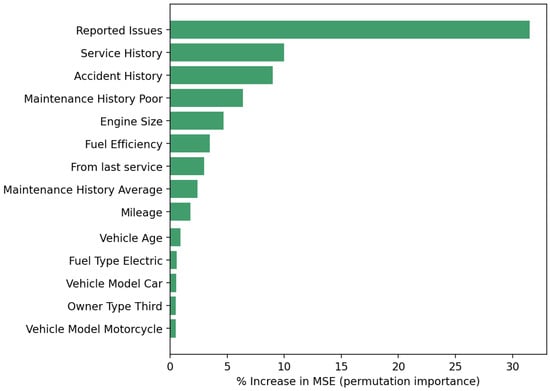
On this basis, a ranking of predictors was constructed using the percentage increase in Mean Squared Error (%IncMSE) metric. This indicates the percentage by which the model’s accuracy deteriorates following a random change in the value of a given variable whilst keeping the others constant. Higher values indicate greater importance of the predictor for prediction quality. The values were calculated based on 5 permutation repetitions on a random sample of 5000 observations from the training set. The results are shown in Figure 2.

Figure 2. %IncMSE plot for the random forest model.

The %IncMSE graph clearly indicates that the variable ‘reported issues’ has the greatest influence on the phenomenon under study (32.78%); next in the ranking of predictors are the variables ‘service history’ (12.23%), ‘accident history’ (9.32%) and ‘maintenance history Poor’ (7.78%), which also have a significant influence. The subsequent predictors, i.e., engine size, maintenance history average, vehicle age, fuel efficiency, time since last service and mileage, achieved values in the range of 3.7–5.9%, and therefore their influence on the phenomenon under study should be described as moderate.

Finally, an XGBoost model was built. The following assumptions were made during the model’s construction:

• number of trees n = 300;
• learning rate = 0.1;
• maximum depth of a single tree—5;
• proportion of observations sampled for each tree—80%;
• number of features sampled during splitting—4;
• minimum number of observations for node splitting—20;
• minimum number of observations in a leaf node—10.

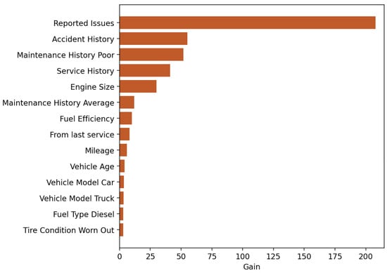
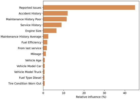
On this basis, a ranking of predictor importance for the model was determined using a Gain chart and a Relative Influence chart. The Gain metric reflects the total reduction in the loss function (log-loss) achieved through splits based on a given variable, summed across all trees and nodes. In contrast, Relative Influence is a normalized version of this measure, expressed as a percentage. The resulting charts are shown in Figure 3 and Figure 4.

Figure 3. Gain chart for the XGBoost model.

Figure 4. Relative influence chart for the XGBoost model.

The Gain chart clearly shows that the variable with the greatest influence on the modeled phenomenon is ‘reported issues’, with a value of 200.00. The next variables in the predictor ranking are ‘accident history’ (55.00), ‘maintenance history poor’ (50.00) and ‘service history’ (40.00).

Based on the Relative Influence plot, which is a normalized version of the Gain plot, it can be concluded that the ‘reported issues’ variable accounts for 45.28% of the total influence of all variables in the model. In contrast, the ‘accident history’ and ‘maintenance history poor’ variables account for 14.84% and 12.52% of the influence, respectively.

4. Discussion

In the next step, the saved logistic regression, classification tree and XGBoost models were applied to the test set to assess their predictive capabilities. Next, a classification matrix was plotted for each model, and the accuracy, recall, specificity and precision metrics were calculated. Metrics for the predictive performance of each model were also calculated. Predicted probabilities were converted into binary classifications using the standard 0.5 threshold, meaning that a vehicle was classified as requiring maintenance (class 1) whenever the model-estimated probability of needing service equaled or exceeded 50%. This default threshold treats false positives (unnecessary interventions) and false negatives (undetected maintenance needs) symmetrically.

In the first step, a classification matrix was constructed for the logistic regression model (Table 8).

Table 8. Classification matrix for the logistic regression model.

	Predicted: 1	Predicted: 0
Observed: 1	9303	2846
Observed: 0	884	1967

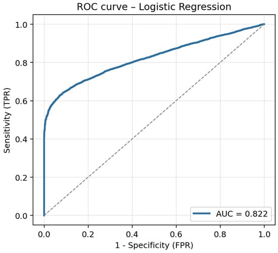
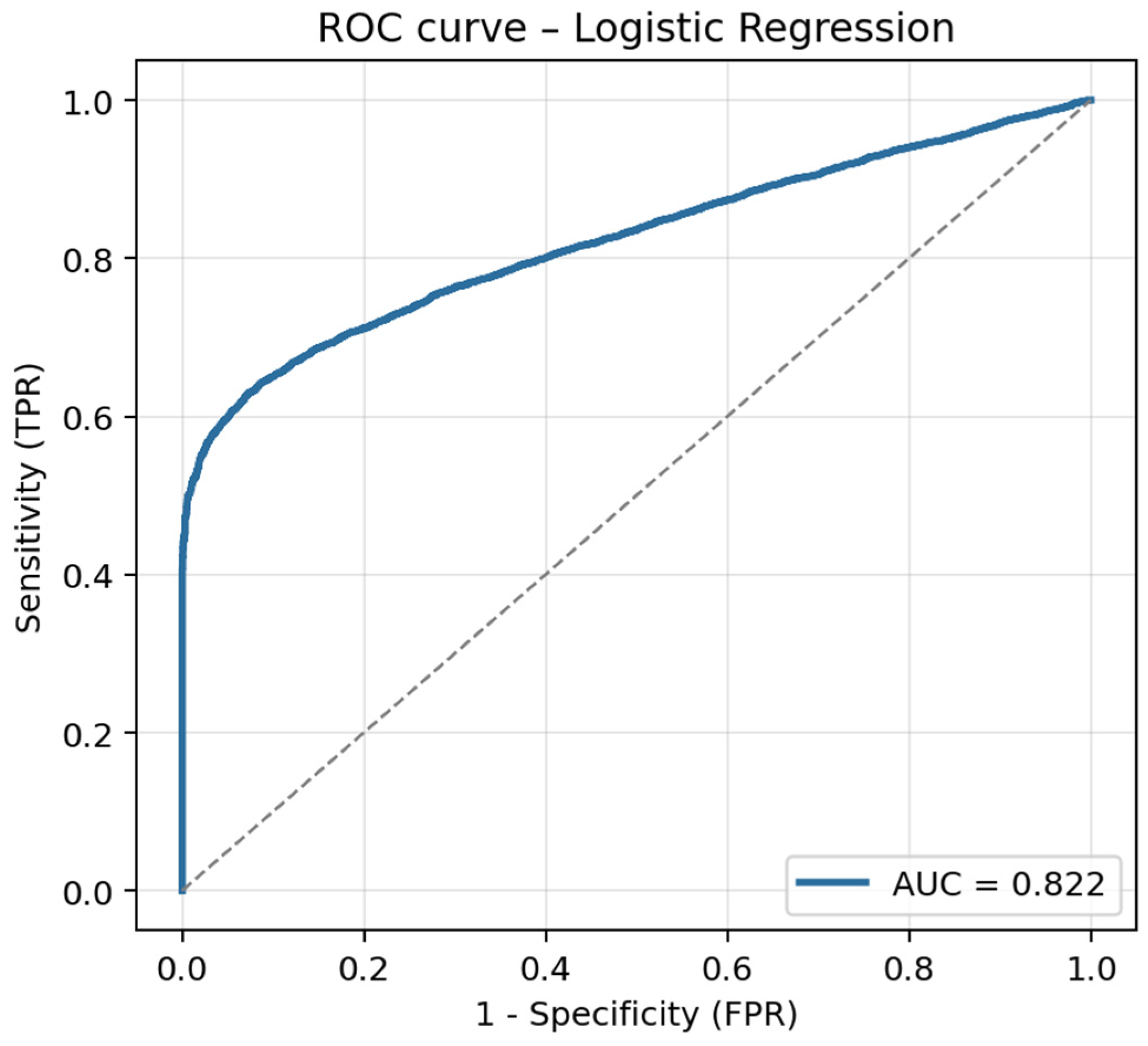
In the next step, the ROC curve was plotted and the AUC was calculated (Figure 5).

Figure 5. ROC curve of the logistic regression model.

Out of 15,000 observations, the model correctly classified 11,270. The calculated AUC value for the logistic regression model was 0.82, indicating good predictive ability.

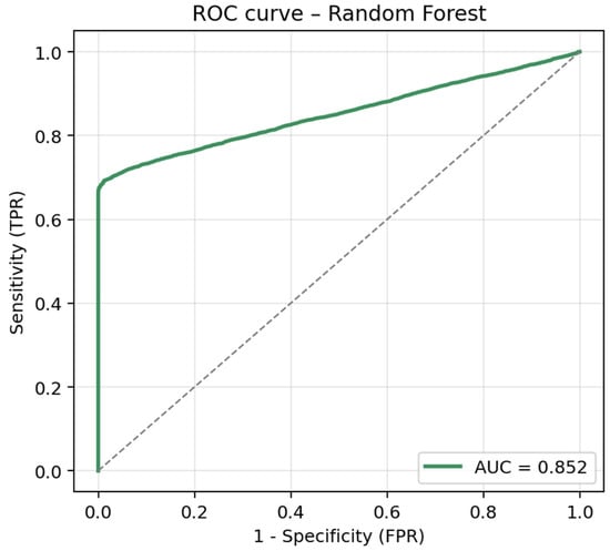
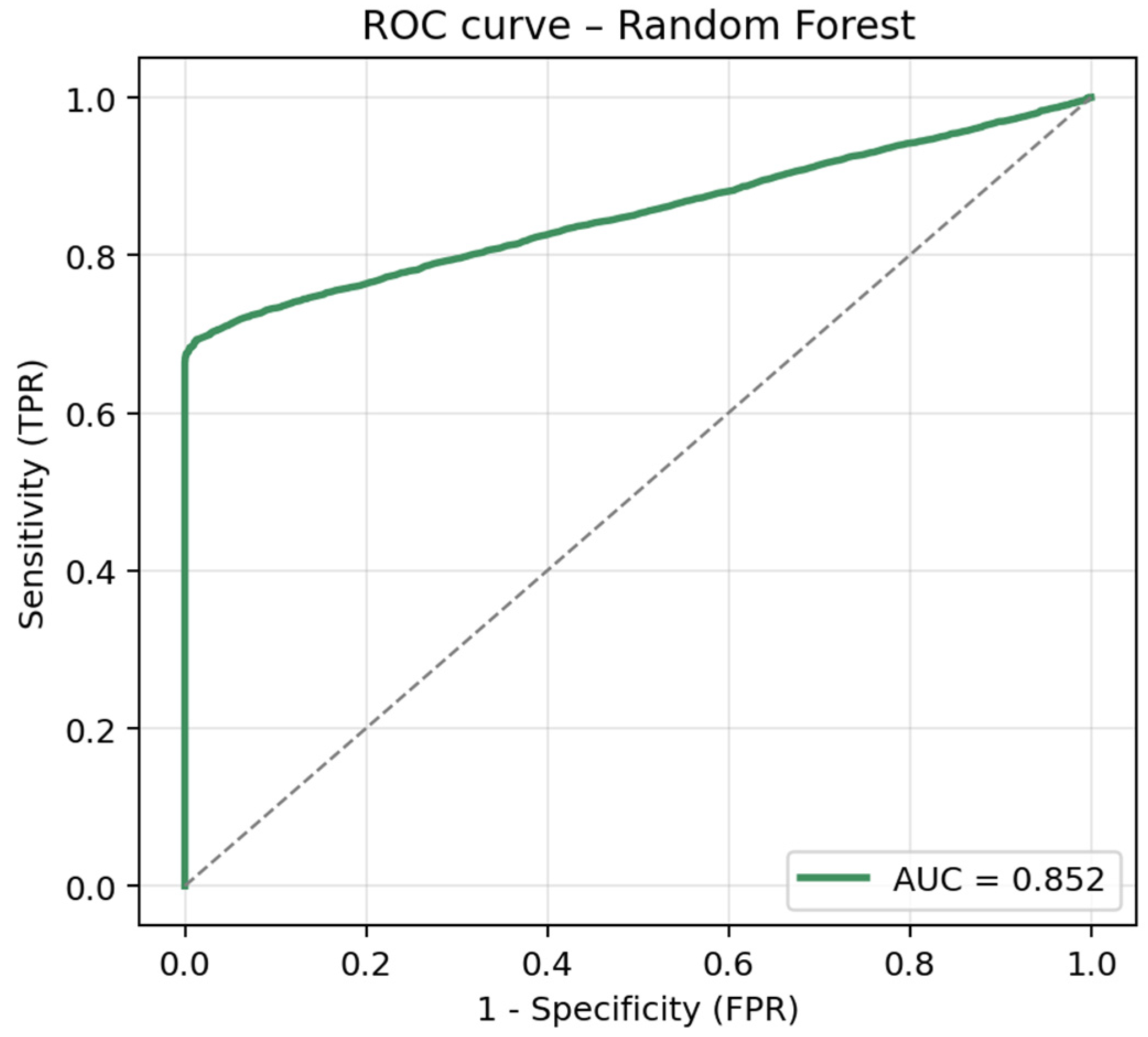
In the next step, the classification matrix and ROC curve were plotted for the random forest model using the random forest algorithm (Table 9 and Figure 6).

Table 9. Classification matrix for the random forest model.

	Predicted: 1	Predicted: 0
Observed: 1	9564	2585
Observed: 0	770	2081

Figure 6. ROC curve for the random forest model.

Out of 15,000 observations, the model correctly classified 11,645, whilst the calculated AUC value for the decision tree model was 0.852, indicating very good predictive ability.

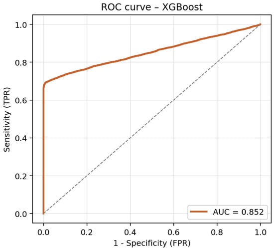
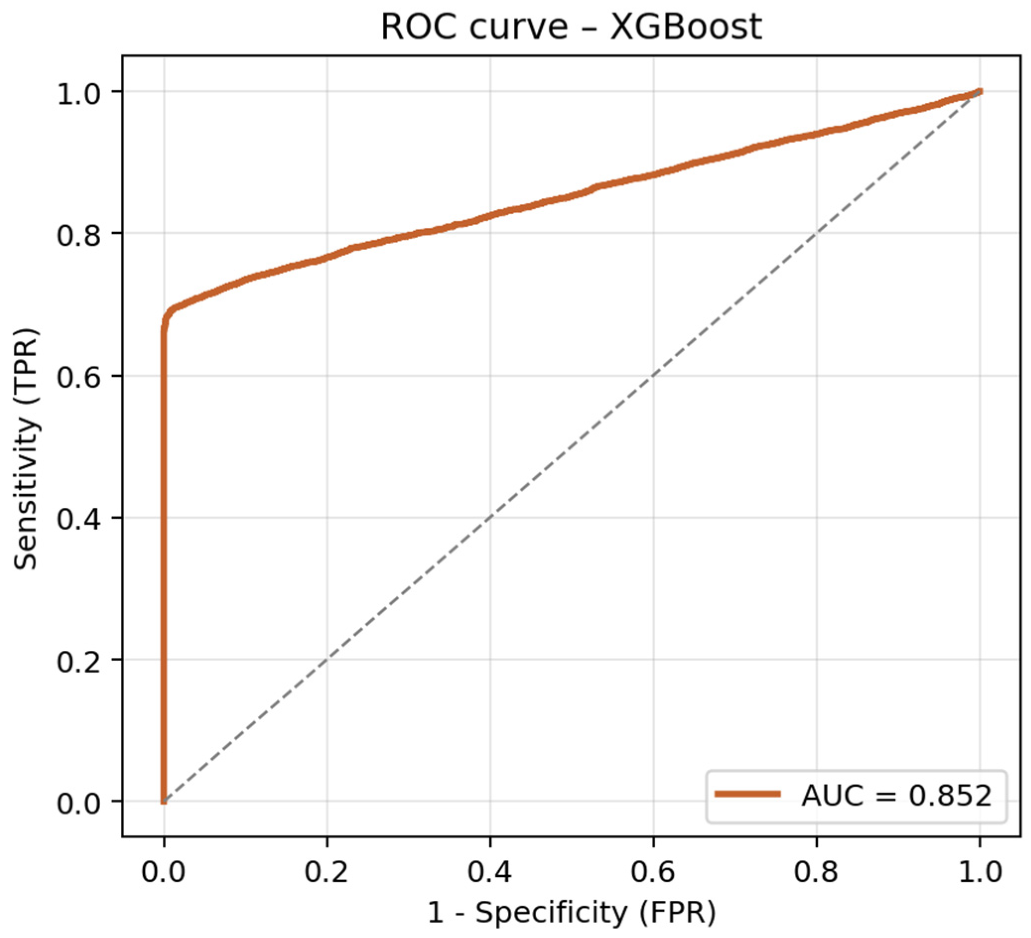
In the final step, the classification matrix and ROC curve were plotted for the XGBoost model (Table 10 and Figure 7).

Table 10. Classification matrix for the XGBoost model.

	Predicted: 1	Predicted: 0
Observed: 1	9656	2493
Observed: 0	833	2018

Figure 7. ROC curve for the XGBoost model.

Out of 15,000 observations, the model correctly classified 11,674. The calculated AUC value for the XGBoost model was 0.852, indicating very good predictive ability.

In the final step, the developed models were compared based on the calculated classification quality metrics and model fit metrics (Table 11).

Table 11. Quality indicators for individual models.

Measure	Logistic Regression	Random Forest	XGBoost
Accuracy	75.13%	77.63%	77.83%
Sensitivity (Recall)	76.57%	78.72%	79.48%
Specificity	68.99%	72.99%	70.78%
Precision	91.32%	92.55%	92.06%
AUC-ROC	0.8219	0.8521	0.8523

A comparative analysis of the three models built—logistic regression, random forest and XGBoost—was carried out on a joint test sample comprising 15,000 observations. A comparative analysis of all calculated quality and fit measures showed that the XGBoost model is the best, slightly outperforming the random forest model. The logistic regression model exhibited the weakest predictive capabilities.

The calculated accuracy was 75.13% for logistic regression, 77.63% for random forest and 77.83% for XGBoost. The sensitivity of the models was 76.57%, 78.72%, and 79.48% respectively. Specificity is the dimension where the differences between the models are most pronounced—logistic regression achieved 68.69%, whilst random forest and XGBoost achieved 72.99% and 70.78% respectively. This means that decision tree models are almost twice as effective at eliminating false alarms, correctly identifying nearly 72% of vehicles that do require technical intervention. The precision of the models was 91.32%, 92.55% and 92.06%% respectively, confirming that decision tree models classify vehicles as maintenance needs with significantly higher reliability than logistic regression. The area under the ROC curve was 0.8219 for logistic regression, 0.8521 for random forest and 0.8523 for the XGBoost model. This demonstrates the good to very good predictive capabilities of the models built.

Based on the results obtained, it should be concluded that the XGBoost model is best suited to the analyzed data. It achieved the highest values for accuracy, sensitivity, and AUC-ROC among all three methods. Of particular significance is the AUC value of 0.8523, which exceeds the threshold recognized in the literature as the boundary for very high discrimination, and the high precision of 92.06%, indicating a low rate of false technical interventions. The sequential nature of the algorithm, involving iterative correction of errors in previous trees in combination with the subsampling applied, allowed for a more effective capture of complex non-linear relationships and interactions between predictors than the other methods used.

The superior performance of the XGBoost model has direct operational implications for fleet maintenance management. In practical terms, higher precision reduces the number of vehicles incorrectly classified as not requiring maintenance, which translates into fewer unnecessary breakdowns and reduces loss of availability for vehicles that could remain in service. At the same time, higher recall means that a larger share of vehicles with an actual maintenance need are correctly identified, allowing potential failures to be addressed earlier and reducing the risk of unexpected breakdowns during operation. By combining these properties, the XGBoost-based decision support can help fleet managers shorten unplanned downtime, stabilize service reliability and allocate maintenance resources more efficiently. Thus, the comparative advantage of XGBoost over random forest and Logistic Regression should be interpreted not only as a statistical improvement, but as a practical contribution to risk-based maintenance planning and fleet readiness. The superior performance of the XGBoost model has direct operational implications for fleet maintenance management. In practical terms, higher precision reduces the number of vehicles incorrectly classified as not requiring maintenance, which translates into fewer unnecessary breakdowns and reduces loss of availability for vehicles that could remain in service. At the same time, higher recall means that a larger share of vehicles with an actual maintenance need are correctly identified, allowing potential failures to be addressed earlier and reducing the risk of unexpected breakdowns during operation. By combining these properties, the XGBoost-based decision support can help fleet managers shorten unplanned downtime, stabilize service reliability and allocate maintenance resources more efficiently. Thus, the comparative advantage of XGBoost over random forest and Logistic Regression should be interpreted not only as a statistical improvement, but as a practical contribution to risk-based maintenance planning and fleet readiness. This interpretation, based on a single split, is revisited below in light of cross-validated robustness checks, formal significance testing, and an operational cost analysis (Table 12, Table 13 and Table 14). It should be noted that in the remainder of the study, the advantage of XGBoost over random forest was not statistically confirmed, and the preferred model depends on the relative costs to the fleet operator of missed or unnecessary interventions.

Table 12. Cross-validated performance metrics (mean ± SD across 5 stratified folds).

Measure	Logistic Regression	Random Forest	XGBoost
Accuracy	75.36% ± 0.42	77.69% ± 0.29	77.62% ± 0.29
Sensitivity	77.18% ± 0.59	78.47% ± 0.57	78.86% ± 0.48
Specificity	67.61% ± 0.81	74.36% ± 1.05	72.32% ± 0.99
Precision	91.04% ± 0.18	92.88% ± 0.23	92.39% ± 0.23
F1-score	83.54% ± 0.33	85.07% ± 0.25	85.09% ± 0.24
AUC-ROC	0.8215 ± 0.0028	0.8546 ± 0.0026	0.8528 ± 0.0025

Table 13. Post hoc Wilcoxon signed-rank tests (Holm-corrected p-values) for pairwise model comparisons across 5 folds.

Comparison	Metric	Wilcoxon W	p-Value	Holm-Adjusted p
Random Forest vs. XGBoost	F1	7.00	1.0000	1.0000
Random Forest vs. Logistic Reg.	F1	0.00	0.0625	0.1875
XGBoost vs. Logistic Reg.	F1	0.00	0.0625	0.1250
Random Forest vs. XGBoost	AUC	1.00	0.1250	0.1250
Random Forest vs. Logistic Reg.	AUC	0.00	0.0625	0.1250
XGBoost vs. Logistic Reg.	AUC	0.00	0.0625	0.0625

Table 14. Confusion matrix and performance metrics on the held-out test set (15,000 observations) for the final models.

Measure	Logistic Regression	Random Forest	XGBoost
True Negatives (TN)	1971	2162	2126
False Positives (FP)	880	689	725
False Negatives (FN)	2842	2688	2659
True Positives (TP)	9307	9461	9490
Accuracy	75.19%	77.49%	77.44%
Precision	91.36%	93.21%	92.90%
Sensitivity	76.61%	77.87%	78.11%
Specificity	69.13%	75.83%	74.57%
F1-score	83.34%	84.86%	84.87%
AUC-ROC	0.8217	0.8531	0.8514

To assess the robustness of the fixed-hyperparameter configurations described above beyond a single split, all three models (logistic regression, random forest and XGBoost) were additionally evaluated using 5-fold stratified cross-validation applied exclusively to the training set (35,000 observations). For each fold, the SMOTE-based resampling and feature-encoding pipeline described above was re-executed independently on that fold’s training partition only, using a unified, leakage-safe resampling-and-preprocessing architecture. The corresponding validation partition was never resampled, eliminating the risk of information leakage between synthetic and validation observations. For each of the five folds, the fitted pipeline was evaluated using estimations of accuracy, sensitivity, specificity, precision, F1-score and the area under the ROC curve (AUC-ROC). The resulting mean values and standard deviations across folds are reported in Table 12.

Across the five folds, random forest and XGBoost achieved comparable and consistently higher performance than logistic regression on all metrics, with mean AUC-ROC values of 0.8546 and 0.8528 and mean F1-scores of 85.07% and 85.09%, respectively. Random forest exhibited a modestly higher and more stable specificity (74.36% ± 1.05) than XGBoost (72.32% ± 0.99), indicating a lower and more consistent false-positive rate across folds, whereas XGBoost showed a marginally higher sensitivity (78.86% ± 0.48 vs. 78.47% ± 0.57). The narrow standard deviations observed for all three models (typically below one percentage point, with the exception of XGBoost’s specificity) suggest that the performance estimates are stable across different partitions of the training data and are not driven by a particular, possibly favorable, train–test split. Whether the small differences observed between random forest and XGBoost are statistically significant is formally assessed later in this study using the Friedman and Wilcoxon signed-rank tests.

To formally assess whether the performance differences observed across the five cross-validation folds (Table 12) are statistically significant, or whether they may plausibly be attributed to sampling variability, a Friedman test was performed separately for the F1-score and the AUC-ROC, treating the three models (logistic regression, random forest, XGBoost) as related samples measured on the same five folds. Where the Friedman test indicated an overall significant difference among the three models, pairwise post hoc comparisons were carried out using the Wilcoxon signed-rank test, with Holm–Bonferroni correction applied to control the family-wise error rate across the three pairwise comparisons.

The Friedman test indicated a statistically significant overall difference among the three classifiers for both F1-score (χ²(2) = 7.60, p = 0.022) and AUC-ROC (χ²(2) = 8.40, p = 0.015), confirming that model performance was not homogeneous across the three algorithms. Post hoc Wilcoxon signed-rank tests (Holm-corrected) are summarized in Table 13.

None of the pairwise post hoc comparisons reached conventional statistical significance (α = 0.05) after Holm correction, including the random forest vs. XGBoost comparison for either metric (F1: p = 1.0000; AUC: p = 0.1250). This should be interpreted with an important caveat: with only five paired observations per comparison, the Wilcoxon signed-rank test has very limited statistical power—its smallest attainable two-sided p-value is 0.0625, which already exceeds the 0.05 threshold even when a model outperforms another consistently in all five folds (as observed for random forest and XGBoost relative to logistic regression). The significant Friedman result therefore indicates a genuine overall difference among the three classifiers, but the present study, limited to 5 outer folds for computational reasons, is underpowered to formally confirm which specific pair of models drives that difference. In particular, the numerically small gap between random forest and XGBoost observed in Table 12 (mean F1 difference of 0.02 percentage points; mean AUC difference of 0.18 percentage points) should not be interpreted as statistically confirmed evidence that one model is superior to the other.

In the final step, each of the three pipelines (SMOTE, feature encoding/scaling and classifier, with the fixed hyperparameter configurations described above) was re-fitted once on the entire training set (35,000 raw observations) and evaluated exactly once on the previously untouched test set (15,000 observations). This single, final evaluation—rather than the repeated fold-level evaluations used in Table 12—provides the confusion matrices and operational cost estimates reported below. The test set was not used at any earlier stage of model selection, hyperparameter configuration or robustness checking. The same hyperparameter configuration and the same 70:30 split are used here as in the single-fit models reported in Table 8, Table 9, Table 10 and Table 11.

Beyond standard classification metrics, the practical consequence of each error type differs substantially in a fleet-maintenance context: a false negative (FN) corresponds to a missed maintenance need, which may lead to an unplanned breakdown, whereas a false positive (FP) corresponds to an unnecessary maintenance inspection, incurring a smaller, avoidable operational cost. Denoting the unit cost of a missed failure as the cost of an FN (cFN) and the unit cost of an unnecessary intervention as the cost of an FP (cFP), the total operational cost of a model is:

$$Totalcosts=FN·cFN+FP·cFP$$

(15)

Comparing random forest and XGBoost—the two models not statistically distinguished in the preceding analysis—XGBoost produced 29 fewer false negatives than random forest (2659 vs. 2688), i.e., fewer missed maintenance events, but 36 more false positives (725 vs. 689), i.e., more unnecessary inspections. Setting the two models’ total costs equal yields a break-even cost ratio of 1.24. It should be interpreted that if the cost of a missed failure exceeds roughly 1.24 times the cost of an unnecessary inspection, XGBoost is the more economical choice overall. However, if the ratio is lower than this, random forest is preferable. Because this break-even ratio is of the same order of magnitude as, but not exactly equal to, 1, the practical cost ranking between the two models remains sensitive to the assumed relative costs and should be established using the fleet operator’s own cost data rather than assumed as a fixed property of either algorithm. Logistic regression is dominated by both other models on every criterion (more false negatives and more false positives simultaneously) and is therefore not cost-competitive under any realistic cost ratio.

5. Conclusions

In summary, as part of this study, three predictive models were developed and evaluated, which were then used to assess the need to send a vehicle from the transport fleet for servicing, based on technical and operational data. Logistic regression, a random forest classification model and an XGBoost model were employed. The results of the analysis showed that all three approaches achieved good predictive performance, with random forest and XGBoost both clearly outperforming logistic regression. Between the two ensemble methods, results were mixed and closely matched: XGBoost attained the highest sensitivity, while random forest attained marginally higher accuracy and AUC-ROC in the final test-set evaluation (Table 14), together confirming the suitability of both ensemble methods for classifying vehicles requiring technical intervention. Cross-validated significance testing, however, indicates that the difference between random forest and XGBoost is not statistically significant, and the choice between the two should be informed by the operational cost analysis presented above.

From a research perspective, it is significant that incorporating operational and technical indicators derived from a real-world fleet database into the construction of predictive models enables an accurate estimation of maintenance requirements under conditions of operational uncertainty. A comparison of logistic regression, the random forest model and XGBoost—all built on an identical dataset using a common set of validation metrics—enables an effective assessment of the model’s predictive and interpretative capabilities. In this way, the article fills a research gap in the field of diagnosing maintenance needs based on technical condition analysis and predictive maintenance in transport. The study identifies which classification algorithms are particularly useful when only structured fleet data from TMSs is available, rather than data streams from advanced sensors.

From a practical perspective, the results suggest that they can serve as a basis for transport fleet managers to develop dedicated strategies aimed at reducing unplanned downtime and maintenance costs by prioritizing vehicles based on predicted maintenance requirements, determined from recorded technical and operational data. The analysis also enables the identification of variables that have the greatest impact on a vehicle’s eligibility for maintenance and which, consequently, should be monitored and reported with particular care within the transport management system. Although the study was based on data from a single transport and services company, the proposed modeling framework and data requirements can also be adapted for use in other logistics fleets and by urban and public transport operators. The only limitation in this regard is the availability and recording of similar data within TMSs. A further methodological limitation concerns the number of cross-validation folds used to assess model robustness: for computational reasons, the present study relied on 5-fold cross-validation, which limited the statistical power available to formally distinguish between random forest and XGBoost. A repetition of this procedure with a larger number of folds (e.g., 10-fold or repeated 5 × 10-fold cross-validation, as originally planned) is recommended in future work to obtain adequate statistical power for this comparison. These limitations point to an area for future research, in which analyses should be carried out on larger and more diverse fleets in order to assess the generalisability of the results and to refine tools supporting decision-making regarding condition-based maintenance.

The analyses carried out enabled the unambiguous identification of key predictive variables from the perspective of maintenance decisions. In both the logistic regression model and the decision tree-based models, the most important variables include reported faults, service history, accident history, and selected operational and design characteristics. Similarities in the ranking of the importance of predictive variables between the random forest and XGBoost models confirm the reliability of the conclusions regarding the mechanisms of technical wear and tear in vehicles.

This study fills a gap identified in the literature review on modeling and forecasting maintenance requirements in the transport sector by utilizing classification algorithms that have, to date, been used less frequently. Demonstrating the superiority of the XGBoost model over logistic regression and classification using a random forest model, whilst maintaining the interpretability of the main predictive variables, expands the state of knowledge regarding the use of advanced machine learning methods to predict vehicle maintenance requirements. These results are consistent with the current literature reviews on predictive maintenance in transport, highlighting the growing importance of gradient boosting models in the analysis of large, heterogeneous fleet datasets. As established above, however, the performance gap specifically between XGBoost and random forest was not statistically significant; the two ensemble methods are best regarded as comparably strong alternatives, with the final choice between them left to the operational cost analysis presented earlier.

The developed models also provide a coherent basis for linking technical diagnostics with the logistics decision-making process across several related areas. In maintenance planning, the classification results enable a shift away from rigid schedules based solely on time or mileage towards risk-based planning, in which the frequency and timing of interventions depend on the predicted level of risk for a specific vehicle, rather than on a uniform schedule for the entire fleet. This, in turn, has a direct impact on fleet availability. Correctly identifying vehicles that are highly unlikely to require maintenance (e.g., high specificity in the XGBoost model) reduces the number of units unnecessarily taken out of service, thereby increasing the number of vehicles available to carry out transport tasks. The classification results can also be used when planning the procurement of spare parts. Early identification of vehicles at increased risk of breakdown, combined with information on key variables (reported faults, service history, accident history), enables workshops to better forecast demand for specific components and adjust stock levels accordingly.

In terms of costs, the combination of high precision and specificity reduces the number of unnecessary technical interventions, thereby lowering labor and parts costs for vehicles that do not actually require servicing. At the same time, an appropriate level of sensitivity facilitates the early detection of genuine maintenance needs, thereby reducing the risk of costly, unplanned repairs carried out only after a breakdown occurs during transport operations. From the perspective of service reliability, the ability to anticipate maintenance needs before a fault occurs translates into more stable transport operations and fewer disruptions to delivery times resulting from unplanned downtime.

It should be emphasized, however, that the study has certain limitations which must be taken into account when interpreting the results. The analyses were carried out on a single cross-sectional database with a defined structure of variables, which limits the possibility of directly transferring the models to fleets with different operational profiles, vehicle structures or incident reporting standards. Furthermore, a simple, binary classification of maintenance requirements was adopted, without distinguishing between the type and urgency of the intervention. Model robustness was assessed via 5-fold stratified cross-validation rather than a single data split (Table 12); however, the number of outer folds remains lower than the 10-fold design commonly recommended in the literature, and the reported hyperparameters were fixed rather than tuned through an exhaustive inner-loop search, as discussed above. Additionally, the classification threshold was fixed at the conventional 0.5 value rather than being optimized (e.g., via Youden’s index or cost-sensitive analysis). Given the class imbalance and the asymmetric practical costs of missed versus unnecessary maintenance interventions, a tailored threshold could further improve the operational usefulness of the models and should be explored in future work.

In future work, it would therefore be worthwhile to apply a more comprehensive cross-validation (e.g., 10-fold) and to extend the analysis to include sequential models utilizing time-series data from on-board sensors and telematics systems. This will enable more accurate forecasting of maintenance requirements and a more detailed description of wear dynamics over time. It is also worth assessing the effectiveness of the models discussed from a multi-criteria perspective, covering not only binary maintenance decisions but also the estimation of intervention costs, predicted downtime and the impact of maintenance decisions on key logistics performance indicators. Another area of research is the integration of predictive models with tools for optimizing maintenance schedules and workshop resource management, which will enable the full potential of predictive maintenance to be realized under the actual operating conditions of transport fleets.

References

- Vaidya, S.; Ambad, P.; Bhosle, S. Industry 4.0—A Glimpse. Procedia Manuf. 2018, 20, 233–238. [Google Scholar] [CrossRef] [Scilit]
- Gale, N. Global Trade Disruptions and Domestic Delivery: How Fleets Can Prepare. Available online: https://www.wexinc.com/resources/blog/fleet-strategies-global-trade-disruptions/ (accessed on 20 February 2026).
- Platform Science. The Hidden Costs of Vehicle Downtime and How to Avoid Them. Available online: https://www.platformscience.com/blog/the-hidden-costs-of-vehicle-downtime-and-how-to-avoid-them (accessed on 20 February 2026).
- Clarus. Vehicle Downtime Costs Fleets £800 Per Day—How Can It Be Prevented? Available online: https://clarusprotect.com/vehicle-downtime-costs-fleets-800-per-day-how-can-it-be-prevented/ (accessed on 21 February 2026).
- Wycks, W. The Real Cost of Vehicle Downtime for Your Fleet. Available online: https://www.chevinfleet.com/learning-zone/the-real-cost-of-vehicle-downtime-for-your-fleet/ (accessed on 21 February 2026).
- Krishnan, S.K. Increasing the visibility of hidden failure costs. Meas. Bus. Excell. 2006, 10, 77–101. [Google Scholar] [CrossRef] [Scilit]
- Anderson, L. Preventive Maintenance vs. Reactive Maintenance: Costs, ROI & Best Practices. Available online: https://www.re-leased.com/property-operations/preventive-maintenance-vs.-reactive-maintenance-costs-roi-best-practices (accessed on 3 March 2026).
- Predictive vs Reactive Maintenance: Cost Analysis Guide. Available online: https://oxand.com/en/predictive-vs-reactive-maintenance-cost-analysis-guide/ (accessed on 3 March 2026).
- Celestin, M. How Predictive Maintenance in Logistics Fleets Is Reducing Equipment Downtime and Operational Losses. Brainae J. Bus. Sci. Technol. 2023, 7, 1023–1033. [Google Scholar] [CrossRef]
- EN 13306:2017; Maintenance. Maintenance Terminology. British Standards Institution (BSI): London, UK, 2020.
- Er-Ratby, M.; Kobi, A.; Sadraoui, Y.; Kadiri, M.S. The Impact of Predictive Maintenance on the Performance of Industrial Enterprises. SN Comput. Sci. 2025, 6, 73. [Google Scholar] [CrossRef] [Scilit]
- Molęda, M.; Małysiak-Mrozek, B.; Ding, W.; Sunderam, V.; Mrozek, D. From Corrective to Predictive Maintenance—A Review of Maintenance Approaches for the Power Industry. Sensors 2023, 23, 5970. [Google Scholar] [CrossRef] [Scilit] [PubMed]
- Ali, A.; Abdelhadi, A. Condition-Based Monitoring and Maintenance: State of the Art Review. Appl. Sci. 2022, 12, 688. [Google Scholar] [CrossRef] [Scilit]
- Jardine, A.K.S.; Lin, D.; Banjevic, D. A review on machinery diagnostics and prognostics implementing condition-based maintenance. Mech. Syst. Signal Process. 2006, 20, 1483–1510. [Google Scholar] [CrossRef] [Scilit]
- Garcia, J.; Rios-Colque, L.; Peña, A.; Rojas, L. Condition Monitoring and Predictive Maintenance in Industrial Equipment: An NLP-Assisted Review of Signal Processing, Hybrid Models, and Implementation Challenges. Appl. Sci. 2025, 15, 5465. [Google Scholar] [CrossRef] [Scilit]
- Bampoula, X.; Nikolakis, N.; Alexopoulos, K. Condition Monitoring and Predictive Maintenance of Assets in Manufacturing Using LSTM-Autoencoders and Transformer Encoders. Sensors 2024, 24, 3215. [Google Scholar] [CrossRef] [Scilit] [PubMed]
- Benhanifia, A.; Cheikh, Z.B.; Oliveira, P.M.; Valente, A.; Lima, J. Systematic review of predictive maintenance practices in the manufacturing sector. Intell. Syst. Appl. 2025, 26, 200501. [Google Scholar] [CrossRef] [Scilit]
- O’Neil, R.; Khatab, A.; Diallo, C. Optimizing predictive maintenance and mission assignment to enhance fleet readiness under uncertainty. Auton. Intell. Syst. 2025, 5, 17. [Google Scholar] [CrossRef] [Scilit] [PubMed]
- Ando, M.D.N.; Zakrzewski, B.; Dul, I. Artificial Intelligence in the Management of Transportation Companies. Eur. Res. Stud. J. 2026, 29, 432–447. [Google Scholar] [CrossRef] [Scilit]
- Gayialis, S.; Kechagias, E.; Konstantakopoulos, G.D.; Papadopoulos, G. A Predictive Maintenance System for Reverse Supply Chain Operations. Logistics 2022, 6, 4. [Google Scholar] [CrossRef] [Scilit]
- Mahiyudin, G.; Hussain, M.; Dewi, D.D. A Comprehensive Study on Predicting the Need for Vehicle Maintenance Using Machine Learning. Eng. Proc. 2025, 107, 89. [Google Scholar] [CrossRef] [Scilit]
- Makridis, G.; Kyriazis, D.; Plitsos, S. Predictive maintenance leveraging machine learning for time-series forecasting in the maritime industry. In Proceedings of the 2020 IEEE 23rd International Conference on Intelligent Transportation Systems (ITSC), Rhodes, Greece, 20–23 September 2020; pp. 1–8. [Google Scholar] [CrossRef] [Scilit]
- Ahmed, A. Hybrid and deep learning architectures for predictive maintenance: Evaluating LSTM, and attention-based LSTM-XGBoost on turbofan engine RUL. MATEC Web Conf. 2025, 413, 07008. [Google Scholar] [CrossRef] [Scilit]
- Ersöz, O.Ö.; İnal, A.F.; Aktepe, A.; Türker, A.K.; Ersöz, S. A Systematic Literature Review of the Predictive Maintenance from Transportation Systems Aspect. Sustainability 2022, 14, 14536. [Google Scholar] [CrossRef] [Scilit]
- Oszczypała, M.; Ziółkowski, J.; Małachowski, J. Redundancy allocation problem in repairable k-out-of-n systems with cold, warm, and hot standby: A genetic algorithm for availability optimization. Appl. Soft Comput. 2024, 165, 112041. [Google Scholar] [CrossRef] [Scilit]
- Grzelak, M.; Owczarek, P.; Stoica, R.-M.; Voicu, D.; Vilău, R. Application of Logistic Regression to Analyze The Economic Efficiency of Vehicle Operation in Terms of the Financial Security of Enterprises. Logistics 2024, 8, 46. [Google Scholar] [CrossRef] [Scilit]
- Cirneanu, A.-L.; Moldoveanu, C.-E. Use of Digital Technology in Integrated Mathematics Education. Appl. Syst. Innov. 2024, 7, 66. [Google Scholar] [CrossRef] [Scilit]
- Rykała, M.; Grzelak, M.; Rykała, Ł.; Voicu, D.; Stoica, R.-M. Modeling Vehicle Fuel Consumption Using a Low-Cost OBD-II Interface. Energies 2023, 16, 7266. [Google Scholar] [CrossRef] [Scilit]
- Sobczyk, O.W. Modelling Military Equipment Losses with Open-Source Visual Intelligence: Evidence from the War in Ukraine. Mil. Logist. Syst. 2025, 63, 151–164. [Google Scholar] [CrossRef] [Scilit]
- Sokołowski, W.; Ficoń, K.; Florczyk-Żółtowska, M. Data is the fuel of generative artificial intelligence. Mil. Logist. Syst. 2024, 60, 199–216. [Google Scholar] [CrossRef] [Scilit]
- Jaroń, A.; Borucka, A.; Parczewski, R. Analysis of the Impact of the COVID-19 Pandemic on the Value of CO2 Emissions from Electricity Generation. Energies 2022, 15, 4514. [Google Scholar] [CrossRef] [Scilit]
Disclaimer/Publisher’s Note: The statements, opinions and data contained in all publications are solely those of the individual author(s) and contributor(s) and not of MDPI and/or the editor(s). MDPI and/or the editor(s) disclaim responsibility for any injury to people or property resulting from any ideas, methods, instructions or products referred to in the content. |
© 2026 by the authors. Licensee MDPI, Basel, Switzerland. This article is an open access article distributed under the terms and conditions of the Creative Commons Attribution (CC BY) license.