


Abstract
Background: Logistics process development increasingly relies on simulation and artificial intelligence (AI), yet existing approaches provide limited methodological guidance for integrating these technologies throughout the process development lifecycle and selecting economically justified digital maturity levels. Methods: Based on a structured literature review, this study develops an integrated methodological framework covering logistics process development from problem formulation and model design through validation to operational application. The framework assigns algorithm-independent AI functions to individual development stages and combines technical feasibility criteria with discounted net life-cycle cost (NLCC) evaluation to select among digital models, digital shadows and digital twins. Its applicability is illustrated through an industry-inspired proof-of-concept case study involving simulation-based resource optimisation and neural network predictions. Results: The framework establishes a systematic relationship between process development objectives, simulation modelling, AI-based decision support and digital maturity selection. The case study demonstrates how AI can approximate simulation-derived optimal operating parameters to support logistics process improvement. Under the assumed economic conditions, the digital model was the most favourable alternative. Conclusions: The proposed framework provides a structured basis for integrating simulation and AI throughout logistics process development while supporting technically feasible and economically justified decisions.
1. Introduction
The operation of logistics systems is undergoing significant changes as a result of the dynamic technological transformation taking place today. The increasing complexity of supply chains, volatile demand conditions, and growing cost and sustainability expectations require decision support solutions that are capable of capturing and analysing the dynamic behaviour of systems [1]. Process development based on digitalisation technologies is becoming an important competitive factor, as it enables faster and more reliable determination of the system characteristics and variants examined during development [2].
In this environment, simulation modelling and the application of artificial intelligence play a key role in the analysis and development of logistics processes [3]. Simulation modelling—especially discrete event simulation—has long been used as a tool for examining the performance of logistics systems and for evaluating and optimising development alternatives [4,5]. In recent years, artificial intelligence methods such as predictive modelling, optimisation and machine learning have also gained increasing prominence in the field of logistics decision support [6]. There are few studies that integrate these tools into a unified methodological framework specifically designed for logistics process development [7,8]. In particular, there is a lack of consistent interpretation of the maturity levels of digital models, digital shadows and digital twins, and their methodological connection to process development goals and economic evaluation.
The aim of this study is to develop and present a structured, process development-oriented methodological framework that integrates the use of logistics process simulation and artificial intelligence for various development goals. The research seeks to answer the question of how logistics process development can be supported along the digital model, digital shadow and digital twin levels, and what role artificial intelligence can play in decision support at each maturity level. The contribution of the study is fourfold: (i) a unified framework integrating logistics simulation modelling and artificial intelligence within a single process development methodology; (ii) an explicit link between simulation design and the three digital maturity levels, with guidance for selecting the appropriate level by means of a rule-based decision function and a discounted net life-cycle cost (NLCC) criterion that compares alternative maturity levels for a given task rather than appraising a single investment; (iii) the identification of algorithm-independent roles of artificial intelligence along the process development lifecycle (model selection, data preparation, prediction, optimisation, validation and decision support); and (iv) a proof-of-concept illustration of the framework through an industry-inspired case study.
2. Structured Literature Review to Identify Scientific Gaps
A structured, semi-systematic literature review [9] was conducted to explore the development of the field under study and to identify current scientific gaps and opportunities for further development. The review followed a transparent, stepwise search and screening protocol inspired by systematic review guidelines; however, the publications analysed in detail were selected purposively by the author according to the research objectives of this study (see Step 4). Consequently, the review does not claim the exhaustiveness of a full systematic review; rather, it aims to provide a transparent, research-question-driven overview of the field.
Steps in the structured literature review:
- Determining motivation: Simulation modelling and artificial intelligence solutions are undergoing significant transformation. The review aims to explore research directions and gaps related to their integrated application in logistics process development.
- Defining research questions: In analysing the literature on the research topic, this study seeks answers to the following research questions:
- −
- What are the main types and areas of application of simulation modelling and artificial intelligence in logistics?
- −
- What are the objectives of applying these technologies?
- −
- What research directions and gaps can be identified in the field of logistics process development in relation to the integration of the aforementioned technologies?
- Conducting a literature review: The search was conducted in Scopus, selected for its broad coverage of peer-reviewed publications and its widespread use in systematic reviews, on 15 January 2026 and covered all publications indexed up to that date. Keyword combinations were queried in the TITLE-ABS-KEY field (titles, abstracts and keywords); each query listed below was entered in the form TITLE-ABS-KEY (<query>); for example, Search Query 4 was entered as TITLE-ABS-KEY ((“logistics” OR “supply chain”) AND (“simulation”) AND (“artificial intelligence”)). The search queries and the corresponding number of retrieved publications were as follows:
- (“logistics” OR “supply chain”) → 1,044,668 documents
- (“logistics” OR “supply chain”) AND (“simulation”) → 38,628 documents
- (“logistics” OR “supply chain”) AND (“artificial intelligence”) → 15,641 documents
- (“logistics” OR “supply chain”) AND (“simulation”) AND (“artificial intelligence”) → 1175 documents
- (“logistics” OR “supply chain”) AND (“simulation”) AND (“artificial intelligence”) AND (“process improvement” OR “process development”) → 6 documents
As query 5 returned only a few results, further analyses were based on query 4. Figure 1 shows its annual publication counts up to 2025; 2026 is omitted, as the search covered only its first two weeks. Publications rose markedly between 2017 and 2022, driven by the rise of digitalisation and artificial intelligence, and accelerated further to 109 in 2023 and 162 in 2024. The lower 2025 value (74) probably reflects incomplete indexing at the query date.
Figure 1.
Number of publications over time.
Analysis of the metadata shows that research using artificial intelligence and simulation modelling in the field of logistics and supply chains is particularly prominent in China and the USA (Table 1).
Table 1.
Distribution of publications by country.
Keyword co-occurrence was analysed using VOSviewer 1.6.20 [10]. The relationships between the 40 keywords with at least 8 occurrences are illustrated in Figure 2. The network suggests a growing focus on artificial intelligence in recent logistics and supply chain research.
Figure 2.
Keyword analysis using VOSviewer software.
- 4.
- Selection of relevant publications: The 1175 records retrieved by Search Query 4 were complemented by the first 200 relevance-ranked Google Scholar results for the same keyword combination, in line with the recommendation that the first 200–300 Google Scholar results be examined in evidence reviews [11]. After merging and removing duplicates, the author screened the titles, abstracts and keywords of 1198 unique records.
Following the purposive selection described below, 48 publications were retained for full-text review and synthesis (Figure 3).
Figure 3.
Literature selection process.
Publications were included if they addressed logistics or supply chain systems and investigated the application of simulation modelling and/or artificial intelligence in logistics process development. Priority was given to studies that directly contributed to the research objectives defined in Step 2, including the application areas and objectives of simulation modelling and/or artificial intelligence in logistics and their integration at the digital model, digital shadow and digital twin levels. Publications were excluded from further consideration if they were not directly related to logistics or supply chain processes, addressed simulation modelling or artificial intelligence only marginally, or did not provide additional methodological insights relevant to the research questions compared with already selected studies. Where several publications presented similar approaches, preference was given to the most representative, recent and comprehensive contributions.
It should be acknowledged that the search strategy relies on the umbrella term “artificial intelligence” and the general term “simulation”. Consequently, studies that describe their methods exclusively with more specific terms, such as “machine learning”, “deep learning”, “reinforcement learning”, “surrogate model”, “metamodel” or “simulation-based optimisation”, without mentioning artificial intelligence in the title, abstract or keywords may not have been retrieved. This limitation was partially mitigated by the complementary Google Scholar search, which also indexes full texts and grey literature, and by the research-objective-driven selection of publications. As the aim of the review was to identify the main application areas, objectives and research gaps rather than to provide an exhaustive bibliometric mapping, the applied search terms are considered adequate for the purposes of this study.
- 5.
- Summary of examined publications: The separate and integrated applications of simulation modelling and artificial intelligence in logistics are summarised below.
Simulation in logistics: Logistics simulation is a method suitable for realistic modelling of processes and systems, thus enabling the evaluation of changes in their status [12]. Simulation applications in logistics can be interpreted at three levels of digital twin development (Figure 4): digital model, digital shadow and digital twin [13]. The level of development depends on how the two-way relationship between the physical entity/concept and the digital model is realised. The digital model supports the development of the physical entity/concept based on manual data, while the digital shadow automatically collects data from the physical object. In the case of a digital twin, a two-way, automatic data connection is established, which also allows for intervention.
Simulation techniques are widely used in a variety of logistics areas. Among other things, they have been used for resource forecasting in Cuban ports [6], optimising safety stocks [14], for predicting freight train delays [8], and for optimising last-mile delivery [5]. It has also been applied to AGV control [15] and container loading problems [16].
Figure 4.
Digital twin maturity levels (adapted from [13,17]).
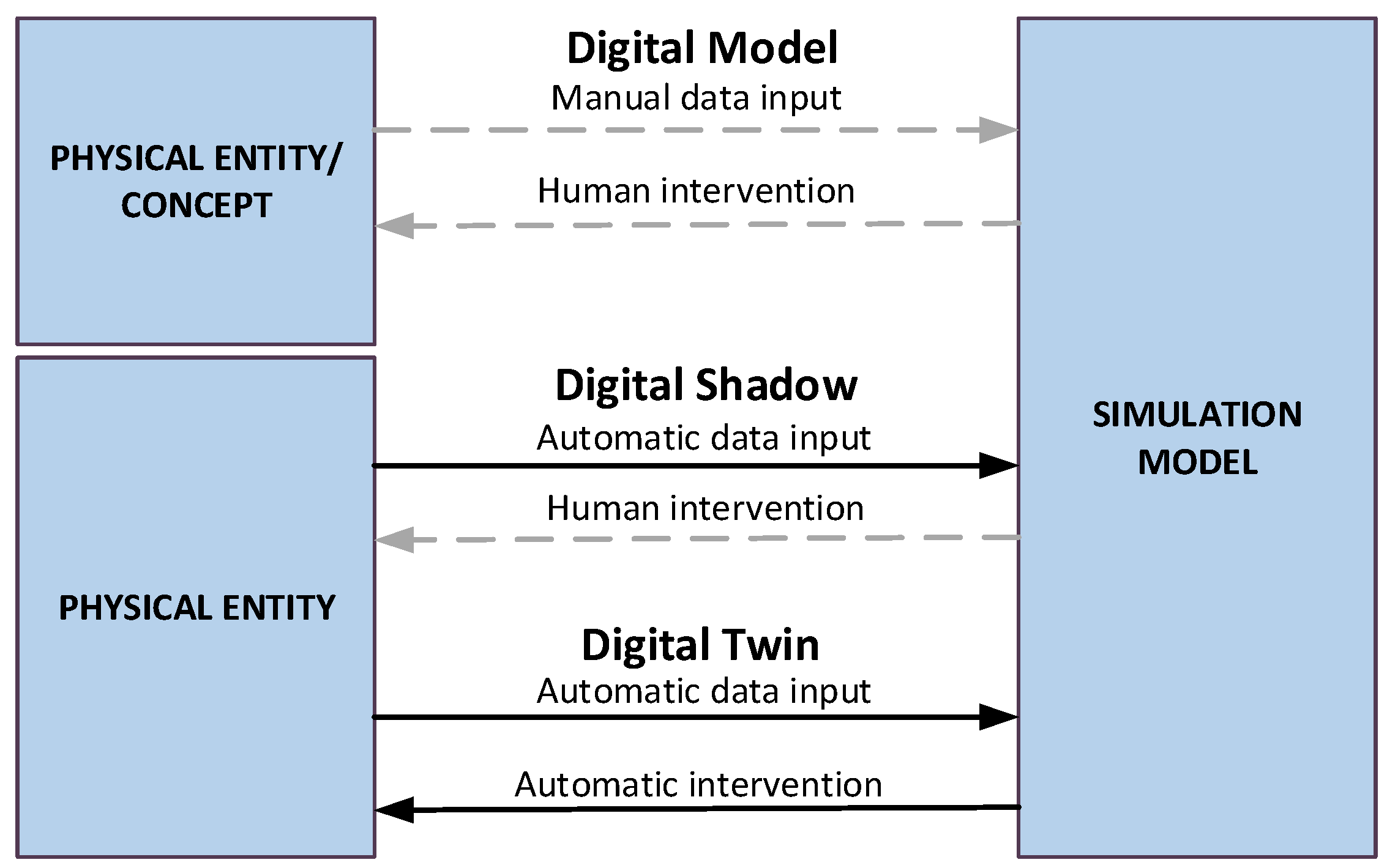
The relevant objectives of simulation modelling are summarised in Table 2.
Artificial intelligence in logistics: Artificial intelligence is a field of computer science concerned with systems capable of performing tasks that require human-like intellectual abilities, such as learning, pattern recognition, problem solving, language comprehension and decision making [18].
Figure 5 illustrates the relationship between Industry 4.0 maturity levels and AI evolution. Level 0 is digitisation using Narrow AI (e.g., AI-based character and voice recognition, etc.). At levels 1–2, AI can support tasks in the areas of visibility and transparency (e.g., image recognition, voice recognition, identifying causes of delays and malfunctions).
Table 2.
Key objectives of simulation application.
Level 3 uses Broader AI, which is capable of learning and making predictions based on the data used (e.g., predictive maintenance, inventory management). At level 4, Broader AI is capable of autonomous decision-making in a specific, well-defined area (e.g., route planning, AMR fleet management). At the theoretical upper levels (5–6), future possibilities such as general logistics artificial advisors or fully autonomous supply networks are emerging. In Figure 5, developed by the author, the maturity levels from visibility to adaptability and the guiding questions assigned to them follow the acatech Industrie 4.0 Maturity Index [23], whose first two stages (computerisation and connectivity) are merged here into level 0 (digitalisation). The assignment of AI types (Narrow AI, Broader AI, AGI and superintelligence) to the levels, the theoretical upper levels 5–6 (general adaptivity and full autonomy) and the distinction between present and future AI evolution are the author’s own extension.
Figure 5.
The relationship between Industry 4.0 maturity levels and AI [own compilation based on [23]].
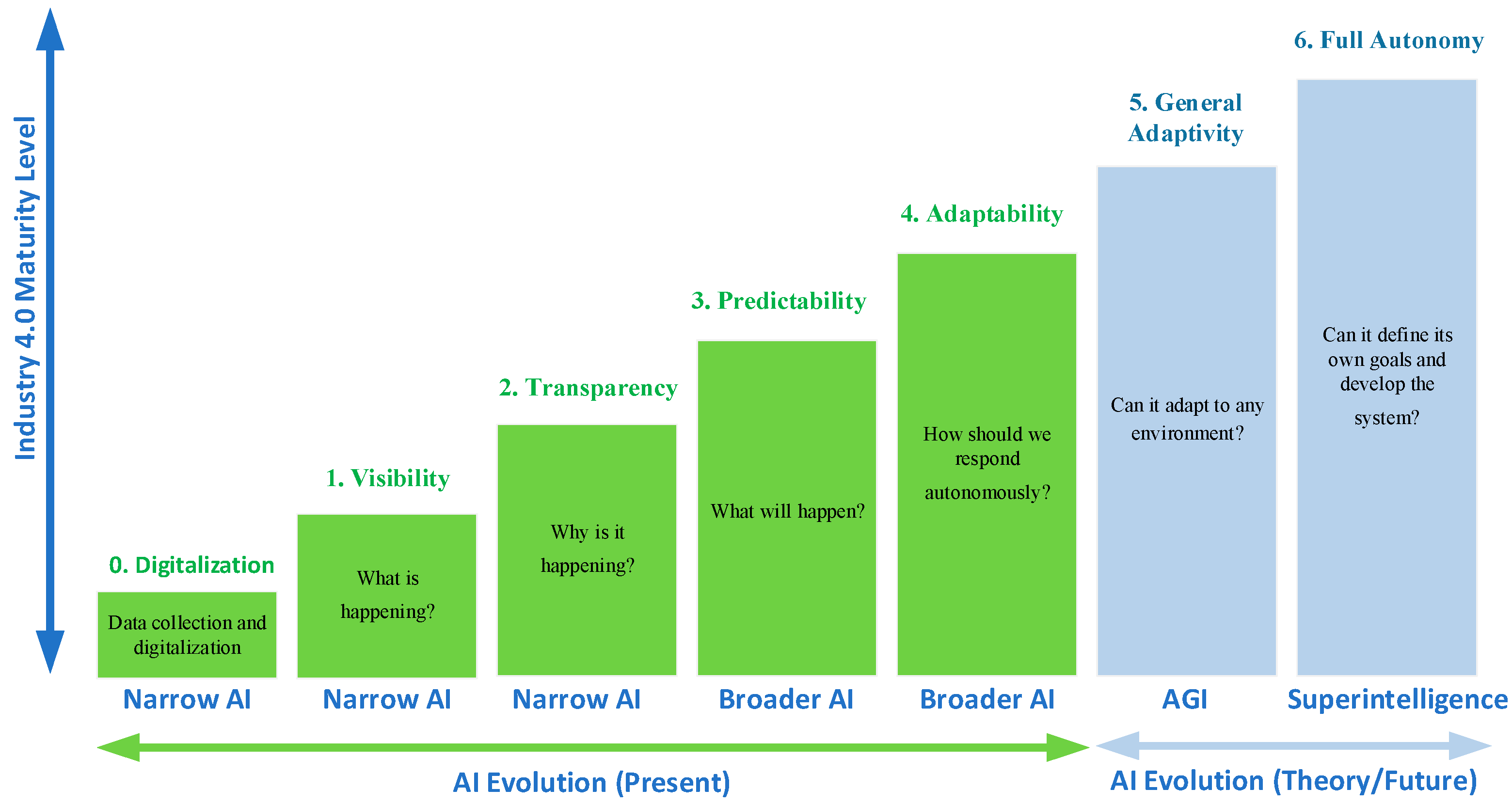
Artificial intelligence (AI) can be widely applied in various areas of logistics, primarily to increase efficiency and reduce costs. AI-based route planning and transport scheduling reduce transport time and CO2 emissions [24]. In warehouse logistics, the control of autonomous guided vehicles (AGVs) using fuzzy logic and genetic algorithms increases operational efficiency [15]. In supply chains, the predictive capabilities of machine learning improve risk management [1]. In predictive maintenance, IoT-based AI systems predict equipment failures, reducing downtime [25]. Furthermore, natural language processing (NLP) can be used to automate the creation of logistics simulation models [4]. Table 3 summarises the relevant objectives of AI application in the field of logistics.
Table 3.
Objectives of AI application.
Logistics simulation and artificial intelligence integration opportunities: The key opportunities for integrating simulation and AI in logistics, together with the related literature, are summarised in Table 4.
Table 4.
Integration opportunities of logistics simulation and artificial intelligence.
- 6.
- Identification of scientific gaps: The reviewed studies report considerable progress in applying simulation modelling, artificial intelligence and digital twin technologies in logistics and supply chain management, e.g., in optimisation, forecasting, scheduling, predictive maintenance and simulation-assisted decision support. However, they generally focus on specific application domains, individual technologies or task-specific combinations rather than on a unified methodological perspective.
Within the scope of the reviewed literature, no methodological framework was identified that systematically integrates logistics simulation modelling, artificial intelligence and digital twin maturity concepts, together with their economic evaluation, into a unified process development methodology covering the complete lifecycle of logistics process development. As the review was based on a purposive selection of 48 publications, this finding is complemented in Section 5.1 by an explicit comparison with the most relevant established reference frameworks: the digital twin classification of Kritzinger et al. [13], Industry 4.0 maturity models [23,40], the CRISP-DM process model [41], and the simulation study and verification and validation frameworks of Banks et al. [42] and Sargent [43]. Two major research gaps were identified:
Gap 1. Although the integration of simulation and artificial intelligence is well documented in the literature (e.g., simulation-based parameter optimisation, surrogate models trained on simulation-generated data, reinforcement learning-based control and AI-enhanced digital twins; Table 4), these solutions typically address a specific task, algorithm or application domain and interpret integration from a technological rather than a process development perspective. A methodology that embeds the combined use of simulation and artificial intelligence into the complete logistics process development lifecycle, from problem formulation through model design, verification and validation to operational application, and that defines the role of artificial intelligence as algorithm-independent functions assigned to specific development steps (model selection, data preparation, prediction, optimisation, validation and decision support) is still lacking.
Gap 2. The distinction between digital models, digital shadows and digital twins is mainly treated in the literature as a descriptive classification or as a technological maturity stage [13,17,23,40]; organisation-level maturity models recommend setting target stages according to company strategy and cost–benefit considerations [23], but they do not provide guidance at the level of an individual task. Within the scope of the reviewed literature, no methodological guidance was found that treats the selection of the maturity level as an explicit design decision and links it to the process development objective, the technical requirements and a life-cycle cost-based economic evaluation accounting for implementation and operating costs as well as avoided losses.
These gaps motivate the proposed framework; the gaps and the corresponding contributions are summarised in Table 5.
Table 5.
Relationship between the identified research gaps and the contributions of the proposed framework.
3. Framework for Logistics Process Development: Integrated Application of Process Simulation and Artificial Intelligence
This section presents an integrated methodological framework for logistics process development based on the coordinated application of process simulation and artificial intelligence. The proposed framework is organised into four methodological phases: (i) problem formulation, (ii) simulation and AI model design, (iii) implementation and validation, and (iv) operational application. Each phase comprises structured activities intended to progressively reduce modelling uncertainty.
3.1. Description of Examination Options
With regard to the development of the logistics process selected on the basis of the specified process development objective, two types of process development methods can be applied, namely internal and outsourcing-based process development (Figure 6). In the case of internal process development, the service provider managing the process under review does not change. In the case of outsourcing-based process development, the entire process or part of the process is outsourced, or the already outsourced activity is reviewed in terms of changing service providers.
Figure 6.
Description of examination options.
The main steps in the implementation of internal and outsourcing-based process development are described in [2]. During process development, various problem-solving methods are used to achieve the specified development goal [44], the effectiveness of which may be increased by digitalisation technologies in three key areas:
- −
- Definition of operational characteristics: More accurate definition of certain characteristics of the system under investigation that are relevant to development using digital solutions reduces the risk of incorrect decisions. For example, determining the size of an inter-operation storage facility for a planned system using a digital model can help minimise investment risks [4].
- −
- Selecting the ideal system variant: Several possible system alternatives may arise during the process development study. Some evaluation criteria (e.g., investment cost) can be determined without digital support, while others (e.g., performance, capacity utilisation) require the use of digital solutions for more accurate determination. Decision-making is typically based on normalisation and weighting methods that take multiple criteria into account [20].
- −
- Determining optimal operating parameters: Taking into account the development objectives and the possibilities of the given operating environment, digital solutions can help determine optimal parameter values with lower risk. An example of this is the optimal departure times and routes for milk runs at a production plant, which requires the use of digital twins and advanced optimisation algorithms [18].
Depending on the task type, digital model, digital shadow or digital twin solutions may be required; this study focuses on their integration with artificial intelligence.
3.2. Description of the Examination Process
The four phases follow a sequential decision logic: the output of each step provides the input for the subsequent one, which supports consistency between simulation model development, AI integration and validation.
Accordingly, when simulation-based methods are required for internal or outsourced logistics process development, the proposed methodology comprises the following steps (Figure 7):
Figure 7.
Methodological Framework for Logistics Process Development.
- Task definition: The process begins with the specification of the task designated as part of the process development activity, which may consist of the following elements:
- −
- 1/A. Defining operational characteristics: The range of logistical indicators required for the process development examination and the method of their production are determined.
- −
- 1/B. Selecting the ideal system variant: The alternatives to be examined are specified, and the examination criteria necessary for the decision and their weighting, as well as the method of producing the result, are defined.
- −
- 1/C. Determination of optimal parameters: This involves specifying an optimisation task, namely which characteristic(s), conditions and objective function(s) need to be optimised. In addition, expectations regarding the method of producing the result are also recorded.
The common basis of the three task types is the simulation mapping of the investigated logistics system. Let x denote the vector of external inputs of the system (e.g., production programme, demands), θ the vector of design and operating parameters, and ξ the vector of random effects. The vector y of logistics indicators determined in task type 1/A and its estimate are:
where g is the mapping implemented by the simulation test model. For a deterministic model, results from a single run, whereas for a stochastic model it can be estimated as the mean of independent replications. Task types 1/B and 1/C build on these estimated indicators.
For task type 1/B (selection of the ideal system variant), the decision can also be described formally. Let J = {1, …, m} denote the set of investigated system variants, K = {1, …, p} the set of evaluation criteria, and xjk the value of the j-th variant with respect to the k-th criterion, which can be determined without digital support or by simulation. The comparability of the criterion values is ensured by min–max normalisation:
where K+ is the set of criteria to be maximised (e.g., throughput, capacity utilisation) and K− the set of criteria to be minimised (e.g., investment cost). The weighted total score of the variants and the selected variant are:
where wk ≥ 0 is the weight of the k-th criterion and .
Task type 1/C (determination of optimal parameters) can be formulated as an optimisation problem based on mapping (1):
where Θ is the set of admissible parameter values, f the objective function and hi the constraints to be satisfied. In the case of several objective functions, these can be combined by weighting—similarly to Equation (3)—or by lexicographic ordering. The optimisation problem formulated in the case study (Section 4) is a specific instance of this formulation, where the parameter is the number of heat treatment baskets (θ = n), the admissible set is Θ = N = {50, 55, …, 90}, and the objective is lexicographic: primarily the production lead time and secondarily the number of baskets.
In addition, the time schedule for the defined task must also be specified, which can be done in the following ways:
- −
- Bound to a specific deadline (e.g., identification of design errors related to an investment by a specified deadline).
- −
- Repeated at regular intervals (e.g., determining storage capacity requirements for the following year at the end of each year).
- −
- When a specific condition is met (e.g., determining the quantity to be ordered after a given stock level is reached).
- −
- With real-time execution (e.g., real-time flight planning).
- 2.
- Delineation of the system under investigation: After the tasks to be performed have been identified, the boundaries of the logistics system under investigation, i.e., the source and sink objects from the perspective of the simulation test model, are determined.
- 3.
- Defining the implementation framework: If the company under review has the simulation experts necessary to perform the specified task(s), they will be involved in the project. In the absence of such experts, an external service provider will be selected and commissioned.
- 4.
- Studying the operation of the examined system: The participants involved in the task will study the task to be performed in detail and familiarise themselves with the operation of the examined system. The examined system may be a concept that has not yet been implemented, a partially modified version of a real system, or a real system. The experts focus on familiarising themselves with the material and information flow processes of the system under examination and its operating rules.
- 5.
- Determining the type of simulation test model: Designing a simulation test model must be preceded by the selection of the appropriate model type; the types applicable to a given problem are summarised in Table 6. Rather than choosing a digital model, digital shadow or digital twin solely on the basis of technological capabilities, the methodology adapts life-cycle costing principles into a discounted net life-cycle cost (NLCC) criterion. Based on Equations (6) and (7), the model type with the lowest NLCC is selected.Table 6. Types of simulation test models.
Discounted net life-cycle cost (NLCC) model: for each simulation test model type i and period t, the following cost and benefit components are considered:
- -
- : the depreciation cost of the environmental infrastructure (e.g., identification technology, camera system, etc.) to be developed for the application of the type i simulation test model in period t, obtained by distributing the investment cost of the infrastructure evenly (straight-line method) over its useful life.
- -
- : the cost of developing and validating the type i simulation test model in period t.
- -
- : the cost of training the type i simulation test model in period t
- -
- : the cost of data preparation, cleaning and validation necessary for the application of the type i simulation test model in period t.
- -
- : the cost of operating the type i simulation test model (resource requirements, maintenance, analysis, evaluation) in period t,
- -
- : losses avoided by using the type i simulation test model (unnecessary inventory, late delivery, etc.) in period t,
- -
- r: discount rate (e.g., interest rate, expected return).
Since the avoided losses are not known with certainty at the time of planning, they should be taken into account as expected values:
where l = 1, …, L is the index of the loss events considered (e.g., excess inventory, delayed delivery), is the probability of occurrence of the l-th event in period t, and is the loss that can be avoided for that event by applying the type i simulation test model.
In practice, CI–CO can be estimated from investment quotations, project budgets, labour hours and operating records. Event probabilities p and avoidable losses w for E[W] can be derived from historical incidents, simulation scenarios or documented expert estimates; uncertainty should be tested by sensitivity analysis.
Let MS denote the set of technically feasible simulation test model types (Table 6). The selection is performed in two steps. First, the discounted net life-cycle cost is determined for each feasible model type:
and then the alternative with the lowest value is selected:
Since the result of the selection may be sensitive to the uncertain input parameters, in particular the discount rate, it is recommended to check the stability of i∗ over a range r ∈ [rmin, rmax]; the decision can be considered robust if i∗ remains unchanged over the entire range.
In the same way, the stability of the selection should also be examined with respect to the cost components, the expected avoided losses and the length of the evaluation period T; in addition, the switching value of the expected avoided losses, i.e., the value at which a higher maturity level would become preferable, can be determined.
Formally, Equation (6) is the negative net present value of the cost and benefit streams of a given model type; the novelty of the NLCC criterion therefore lies not in the discounting technique but in its application. Unlike conventional discounted evaluation, which appraises a single investment against a do-nothing alternative, the NLCC compares mutually exclusive digital maturity levels for the same logistics task, uses cost terms specific to simulation- and AI-based decision tools, quantifies benefits as expected avoided losses estimated by simulation (Equation (5)), and is restricted to the technically feasible alternatives identified by Equations (8) and (9). Furthermore, investment costs and depreciation are treated separately: the infrastructure investment is not charged as a one-off outlay but enters Equation (6) through its annual depreciation (CI), so that alternatives whose infrastructure has a useful life exceeding the evaluation period are not penalised by the undepreciated part of the investment.
Methodological Guideline for Selecting the Digital Maturity Level
Accordingly, before applying the quantitative NLCC-based evaluation, the set of feasible model types is identified according to three decision criteria: (i) the acceptable decision frequency, (ii) the need for automatic data acquisition, and (iii) the need for automatic feedback to the physical system. For criteria (ii) and (iii), the task defines the minimum required maturity level; higher levels are admissible, but whether they are justified is decided by the NLCC criterion.
The minimum maturity level required by the task is expressed as a decision function. Let a ∈ {0, 1} indicate whether the task requires automatic data acquisition from the physical system (a = 1, e.g., because of data volume or latency) and f ∈ {0, 1} whether it requires automatic feedback (f = 1 if the decision is to be executed without human intervention). Then:
where DM denotes the digital model, DS the digital shadow and DT the digital twin. The combination a = 0, f = 1 is not admissible, since automatic feedback cannot be implemented without automatic data acquisition. Applying Equation (8) to the data collection and feedback columns of Table 6 (manual = 0, automatic = 1) assigns a maturity level L(ai, fi) to each model type i. Let Φ denote the set of decision frequencies acceptable for the task (one-off, periodic, conditional or real-time), φi the method of producing results of type i, and IF the set of model types that are technically feasible in the given environment. The set of feasible model types is then:
i.e., all types with an acceptable decision frequency whose maturity level is at least the minimum level required by the task. A type is excluded as technically infeasible if its data acquisition or feedback cannot be implemented in the given environment, e.g., due to insufficient data quality, system complexity or organisational capabilities; these factors are further reflected in the cost components CA, CF and CO of Equation (6).
If MS contains a single model type, it is selected directly; otherwise, the final selection is performed using the NLCC model (Equations (6) and (7)). The range of hardware and software solutions to be used is also defined during the decision-making process.
- 6.
- Designing a simulation test model: This phase is the methodological core of the framework: the model structure, data sources, AI functionalities and the selected digital maturity level are defined in an integrated manner, which is intended to support consistent implementation and validation and to reduce later redesign. The steps for designing the selected test model (see Figure 8) are as follows:Figure 8. Steps in designing a simulation test model.
- I.
- Defining the application framework: The application framework summarises the information gained in the previous steps and defines the following:
- -
- the purpose of the simulation test model; its role in decision support,
- -
- the time period under investigation and the nature of the application (one-off analysis, periodic evaluation, conditional or real-time operation),
- -
- the type of test model to be implemented (digital model, digital shadow, digital twin).
- II.
- Specifying the model boundaries: In this step, the boundaries of the logistics system under investigation are precisely defined. The source and sink points relevant to the simulation model, the processes and sub-processes involved, and the resources included in the study are identified, so that the model contains only elements relevant to the objective.
- III.
- Defining the level of abstraction and detail: In this step, the level of detail and abstraction of the model is determined. The chosen level must be consistent with the purpose of the study and the quality of the available data. In the case of a macro-level study, an aggregated process description is used, while in the case of a micro-level analysis, individual operations, resource relationships and waiting phenomena also appear in the model.
- IV.
- Exploring AI application possibilities: In this phase, it is determined for which elements of the simulation model and for what purpose it is worthwhile to apply artificial intelligence. The role of AI may include forecasting tasks (e.g., estimating demand trends), optimisation (e.g., to improve resource utilisation), and adaptive decision support that takes into account the dynamic operation of the system.
- V.
- Designing the operation of AI components: This step involves designing the detailed operation of the selected artificial intelligence solutions. The types of algorithms to be used, how learning takes place, what input data the AI is based on, what decision proposals the generated outputs contain, and how these are used in the simulation model are determined.
- VI.
- Designing the material flow system: The method of physical/material flow mapping for the simulation test model is defined. During the design process (in line with the chosen level of abstraction), the following must be specified:
- −
- the source and sink points, as well as the process and sub-process elements to be modelled (model boundaries),
- −
- the types and main attributes of movable units (product, unit load, storage device, vehicle, etc.),
- −
- the main process objects (operations/stations, storage/buffers/warehouses) and the material flow connections between them (routes, service logic),
- −
- resources (people, machines, material handling equipment), their capacity and availability characteristics (e.g., shift schedule).
The material flow must allow the defined outputs to be produced during data loading, testing and running.
- VII.
- Designing the information flow system: This step defines the information and data flow structure related to the material flow logic, i.e., what information the model uses and what data it produces, in what form and where, so that the information flow remains transparent and consistent throughout the model life cycle. The following must be specified:
- −
- The range of data structures required for the model to function, such as dispatch and production plans, initial inventory levels, resource parameters, operating time characteristics, and route and rule parameters.
- −
- The origin and method of data production, with particular regard to whether the individual data elements originate from on-site measurements, corporate information systems (e.g., ERP, WMS, MES), and whether data transfer is carried out manually or via an automated data connection.
- −
- Clear recording of input-output correspondence, i.e., determining which model components are parameterised by each input data element and what output data (e.g., performance indicators, event logs, time series) are generated and stored during model execution.
- −
- In the case of artificial intelligence integration, defining where and in what form the training and test data sets relevant to AI are generated in the simulation model, and how the results produced by AI (e.g., predictions, decision proposals) are fed back into the simulation model. In this case, the experimental design of the simulation (run variants, parameter ranges and increments) and the data preparation phase of CRISP-DM [41] (selection, cleaning, construction, integration and formatting of the training data) are planned jointly, so that the simulation generates the data in the form required by the AI component.
- VIII.
- Defining operational algorithms: This step involves recording the control and decision logic of the simulation test model, i.e., a detailed description of the events that trigger the model, the order in which it operates, the rules it follows and the decision points it uses. The aim of this step is to ensure that the model can be clearly formalised and reproduced on the basis of the material flow structure defined in step VI and the information flow established in step VII, and to ensure subsequent implementation, testing, verification and validation.
When defining the operating algorithms, the following elements must be specified:
- −
- Initialisation algorithms: creation of the initial state of the model, including the setting of initial inventory levels, resource states, shift schedules, order stocks and basic parameters based on the defined data structures.
- −
- Entity generation and entry rules: defining the logic according to which movable units (e.g., products, unit loads, vehicles) are created and entered into the model (e.g., scheduling according to dispatch/production plans, distribution functions, event-driven start-up).
- −
- Routing and process sequence algorithms: recording the sequence of process steps, route selection and the handling of alternative routes (e.g., fixed route, rule-based selection, capacity-dependent redirection).
- −
- Serving and resource allocation algorithms: definition of serving rules, priority order, queuing logic, capacity reservation and conflict management (e.g., FIFO/LIFO, prioritised orders, resource scheduling, vehicle and human resource allocation).
- −
- Time management and event management logic: recording how the model updates states based on events, how it handles operation times, transitions, delays, as well as disruptions and extraordinary events (e.g., failure, resource outage, stock shortage, delivery delay).
- −
- Algorithms for training performance indicators: the method, timing and data source for calculating the logistics indicators assigned to the test objective (e.g., lead time, throughput, resource utilisation, inventory levels, delay rate), as well as the form of recording the results (indicator, time series, event log).
- −
- In the case of AI integration, formalisation of intervention points: clear definition of when and in what role the AI component is linked to the operation of the model; for example:
- providing parameters before running (prediction-based parameterisation),
- provides decision recommendations during runtime (rule-based control support),
- or generates and evaluates scenarios iteratively (optimisation or learning cycle).
- IX.
- Defining automatic data connection and system integration: This step is relevant for digital shadow and digital twin simulation test models. With regard to this step, it is necessary to specify how data flow is implemented for each data type between “external” systems (e.g., ERP, WMS, MES) and the simulation test model being created. In the case of digital shadows, a one-way data connection and system integration is required, while in the case of digital twins, a two-way data connection and system integration is required.
- X.
- Defining automatic feedback and intervention mechanisms: A digital twin not only supports decisions but can also intervene automatically in the real logistics system. Accordingly, the decision points and system states that justify intervention, as well as the rules and thresholds that trigger them, are defined. The intervention alternatives that can be initiated by the digital twin and their expected effects are recorded, ensuring controlled operation. The level of automation (proactive, semi-automatic or automatic) and the timing of interventions (real-time, periodic or event-driven) are defined. The effects of the interventions carried out are continuously monitored and fed back into the operation of the digital twin, while safety limits and emergency shutdown conditions are intended to ensure safe operation.
- XI.
- Recording data update and synchronisation principles: Defining the data update and synchronisation principles of the simulation test model ensures a consistent data connection between the simulation test model and the real system. The principles specify the method and frequency of data updates, the range of data types involved, and the rules for handling data inconsistencies and data delays.
- XII.
- Establishing cybersecurity and operational security requirements: This step defines the principles of data management, access control and authorisation, the protection of data communication against unauthorised interference, and the handling of system errors and data omissions. For digital twins, the secure execution of automatic interventions is of particular importance.
- XIII.
- Definition of system-level verification and validation principles: Verification confirms that the model is implemented according to the planned operating logic without errors, while validation assesses the extent to which the model’s outputs represent the operation of the real logistics system. Three complementary levels are distinguished: (i) simulation model verification, confirming that the implemented model correctly represents the intended conceptual design and operating logic; (ii) AI component validation, evaluating the predictive or decision-support performance of the integrated AI models using appropriate performance measures and independent test data; and (iii) integrated system validation, assessing whether the combined simulation and AI solution adequately represents the real system and provides reliable decision support under practical operating conditions. The tests are based on historical data and expert assessments.
- XIV.
- Defining model version and documentation requirements: This step defines the versioning rules for model development, modification and maintenance, ensuring the traceability of modifications, and the mandatory content of the documentation (e.g., model structure, input data and operating logic). It also defines the framework for applying and, if necessary, modifying the model, thereby supporting transparency, reproducibility and knowledge transfer.
- 7.
- Implementation: After the completion of the design phase of the simulation test model, the model is implemented in accordance with points I-XII: the previously defined material flow, information flow and operational algorithms are realised in the selected simulation environment at the specified level of abstraction and detail.
As part of the implementation step,
- −
- the main objects of the model (process steps, resources, storage, routes) are implemented,
- −
- the input parameters and initial states are set,
- −
- the operational and decision algorithms are implemented.
In the case of artificial intelligence integration, the AI components are attached and their data connections and intervention points are established.
- 8.
- Testing and improving the test model: During the testing of the implemented simulation test model, its correctness, stability and consistency are checked based on the description in Step XIII. The purpose of the testing phase is to identify and correct any logical, data management or implementation errors in the model before substantive testing begins.
Testing typically includes the following activities:
- −
- structural testing (e.g., correct execution of processes, identification of dead ends),
- −
- data management testing (e.g., correct interpretation of input data, consistency of outputs),
- −
- extreme value and sensitivity tests,
- −
- in the case of AI integration, checking the responses and stability of AI components.
Based on the test results, the model is iteratively improved and refined. Once the model has been finalised, its documentation is compiled in accordance with Step XIV.
- 9.
- Application of the simulation test system: The actual tests are performed using the tested and refined simulation test model in accordance with the previously defined process development objectives. The model is run under different scenarios, parameter combinations and system states, allowing for the comparison and evaluation of alternative solutions.
During application,
- −
- the test scenarios are defined,
- −
- individual simulation experiments are run,
- −
- relevant performance indicators are recorded and evaluated,
- −
- in the case of AI integration, learning, optimisation or decision support cycles are also implemented.
The results of the simulation test system directly support internal or outsourced process development decisions and support the assessment of the expected effects of the proposed interventions.
4. Case Study on the Integrated Application of Simulation Modelling and Artificial Intelligence
This case study presents the construction and operation of a simulation test model for the forging of automotive products. The model is based on the operating logic of a real industrial system (material flow, operating rules and decision points), whereas its dimensions and operating parameters were modified for confidentiality reasons; all numerical values are therefore fictitious. The company under review has several forging plants that manufacture automotive components, and the number of heat treatment baskets required by these plants varies on a weekly basis. The ideal number of baskets depends on a number of factors and affects both the operating costs and performance of the system. If the number of heat treatment baskets is lower than expected, this increases production lead times, while excess baskets result in unnecessary resource allocation, leading to higher overall heat treatment basket procurement and maintenance costs. The simulation test model, integrated with AI, is used to determine the optimal weekly number of heat treatment baskets. The case study illustrates, as a proof of concept, how the phases of the framework presented in Section 3 can be applied to an industrial logistics process development problem. Owing to the characteristics of the investigated problem, the implementation corresponds to the digital model maturity level; therefore, only those methodological steps that are relevant to this level are executed, while the remaining steps are discussed as future extensions towards digital shadow and digital twin solutions.
- Task definition: Determining the optimal number of heat treatment baskets for the most favourable production lead time for a designated forging plant and its associated production plan. The task is performed once a week during weekly planning. Optimisation must ensure ideal operation and minimise the number of heat treatment baskets and the associated procurement and maintenance costs at the system level.
The problem can be formulated as follows. Let x = (m1, q1, m2, q2, m3, q3) denote the input vector, where mk is the mass of the product manufactured on the k-th forging machine [kg] and qk its weekly production quantity [pcs] (k = 1, 2, 3). The decision variable is the number of heat treatment baskets, n ∈ N, where, based on Table 7, the set of admissible values is N = {50, 55, …, 90}. The set N defines the grid of simulation runs (the training data); the practical decision space consists of the integer values between 50 and 90, for which the neural network interpolates between the grid points, while the rounding of the continuous estimate to an integer is described in Step 8 below. Let LT(n, x) denote the production lead time determined by the simulation test model. The optimal number of baskets can be specified as a lexicographic optimisation problem:
i.e., the primary objective is to minimise the lead time and the secondary objective—for identical lead times—is to minimise the number of baskets and thereby the procurement and maintenance costs. Since the lead time typically saturates as the number of basket increases, an ε-tolerant selection can be applied instead of strict equality: n* = min{n ∈ N: LT(n, x) ≤ (1 + ε)·min{LT(n′, x): n′ ∈ N}}, where ε ≥ 0 is the acceptable relative increase in lead time; for ε = 0, problem (10) is obtained. The ranges and increments defined in Table 7 yield 43 · 53 = 8000 input combinations and 9 possible basket numbers per combination, i.e., a total of 72,000 simulation runs. Accordingly, the training dataset of the neural network is as follows:
Table 7.
Definition of run variants.
The neural network approximates the mapping defined by dataset (11): , , where w is the vector of weights and biases of the network determined by training.
- 2.
- Delineation of the system under investigation: The system under investigation is bounded by the plant’s three forging machines and four shot-blasting machines.
- 3.
- Defining implementation frameworks: The simulation testing system is developed by researchers with relevant professional experience working at the company under investigation.
- 4.
- Studying the operation of the examined system: The aim of this phase is to understand the material and information flow processes of the examined system, as well as its operating rules. The operation is described in Figure 9.Figure 9. Design of the examined logistics system.
The heat treatment baskets arrive from the storage facility marked with ID 1 and are capable of transporting a total product weight of 250 kg. The three forging machines marked with ID 4 are suitable for forging different types of parts, namely products weighing between 1.5–3 kg, 3–4.5 kg and 4.5–6 kg. The weekly production volume is between 6000 and 10,000 pieces. The operating time of this equipment, the size of the tool change series and the associated tool change time do not change, but vary from forging machine to forging machine. The products coming from the forging machine are automatically loaded at positions marked with the identifier 3, taking into account the capacity of the heat treatment basket. The unit loads are then transferred to the heat treatment furnace marked with the number 6 and then to one of the shot-blasting machines marked with the number 7 (there are 4 available). The shot-blasting machines wait for the products from 6 heat treatment baskets and then perform the shot-blasting operation in 20 min. After shot blasting, the products are transferred to the finished product warehouse marked with the number 8.
- 5.
- Determination of the type of simulation test model: The simulation test model type was selected in two steps: first, the set of technically feasible model types was determined by the rule-based preselection (Equations (8) and (9)) on the basis of the defined test objectives, the characteristics of the investigated logistics process and Table 6; then, the economically most favourable type was selected from this set using the NLCC model. The weekly planning task accepts only periodic execution and requires neither automatic data acquisition nor automatic feedback (Φ = {periodic}, a = f = 0); hence, the minimum required level is the digital model, and MS = {3, 4, 5}. Since MS contains more than one technically feasible type, the final selection was performed using the NLCC model.
Types 1 and 2 are intended for one-off application and are therefore not considered in this case. The calculation was performed over a time horizon of T = 3 years with annual periods, a discount rate of r = 8% and illustrative (fictitious) cost data [EUR/year; where two values are given, the first refers to year 1 and the second to years 2–3]. The infrastructure costs are included as annual straight-line depreciation rather than as a one-off investment outlay: the infrastructure investment of 60,000 EUR for type 4 and 100,000 EUR for type 5 is depreciated over a useful life of 5 years, so only the depreciation attributable to the evaluation period is charged; type 3 requires no additional infrastructure. For type 3, CI = 0, CF = 18,000/3000, CE = 1000, CA = 6000 (manual data preparation), CO = 4000 and E[W] = 30,000; for type 4, CI = 12,000, CF = 30,000/4000, CE = 1500, CA = 2500, CO = 6000 and E[W] = 34,000; for type 5, CI = 20,000, CF = 45,000/6000, CE = 2000, CA = 2500, CO = 8000 and E[W] = 38,000.
Based on Equation (6), NLCC3 ≈ −27,345 EUR, NLCC4 ≈ 3457 EUR and NLCC5 ≈ 37,400 EUR; thus, according to Equation (7), i∗ = 3, i.e., type 3 is selected as the simulation test model. The negative value indicates that, for type 3, the present value of the avoided losses exceeds the present value of the costs. The additional benefit of the higher maturity levels (the increase in E[W]) does not cover the infrastructure and development costs of automatic data connection and feedback, which is consistent with the fact that the weekly planning task does not require a real-time data connection. The selection remains unchanged over the range r ∈ [4%, 12%] (NLCC3 ≈ −29,978 … −25,036 EUR); hence, within the illustrative data, the decision is robust with respect to the discount rate. The selection also remains unchanged when all cost components are varied by ±30% (NLCC3 ≈ −42,335 … −12,354 EUR; NLCC4 ≈ −23,866 … 30,781 EUR), when the expected avoided losses are varied by ±30% (NLCC3 ≈ −50,539 … −4151 EUR; NLCC4 ≈ −22,829 … 29,744 EUR), and when the evaluation period is varied between T = 2 and 5 years, i.e., up to the useful life of the infrastructure (NLCC3 ≈ −49,994 … −14,643 EUR; NLCC4 ≈ −7868 … 9808 EUR); type 5 remains the least favourable alternative in all cases. Type 4 would become preferable only if its expected avoided losses exceeded approximately 45,950 EUR/year (about 35% above the assumed value), and type 5 only above approximately 63,100 EUR/year (about 66% above the assumed value).
- 6.
- Designing the simulation test model: This step follows the design steps of Figure 8, which decomposes Step 6 of Figure 7; at the digital model level, steps IX, X and XII are not relevant.
- I.
- Defining the application framework: The aim of the simulation test is to determine the optimal number of heat treatment baskets used in a forging plant by minimising the production lead time and, as a secondary objective, the number of baskets. The test covers a weekly planning period and serves as a decision support tool for production planning.
- II.
- Specifying the scope of the model: The simulation study covers the technological process of the forging plant from forging machines to shot-blasting equipment, including inter-operation storage and the heat treatment process. The study does not cover raw material supply and finished product delivery.
- III.
- Definition of the level of abstraction and detail: The model describes the main resources and material flow relationships of the technological process under investigation using a discrete event simulation approach. Human resources are not explicitly modelled; their impact is aggregated in the technological times.
- IV.
- Exploration of AI application possibilities: In line with the objective of the study, artificial intelligence is applied using a neural network-based approach to facilitate decision support. The task of the neural network is to estimate the optimal number of heat treatment baskets and the associated production lead time based on the input parameters associated with the given system settings. The input layer contains the product mass and production volume data associated with the three forging machines, while the neurons in the output layer represent the optimal number of heat treatment baskets and the production lead time.
It should be emphasised that the case study is intended to demonstrate the proposed process development methodology rather than to identify the best-performing AI method. The framework is method-agnostic with respect to the AI component: the selection of the AI method is itself a step of the framework (Step IV), and the neural network applied here is one interchangeable option that could be replaced by, for example, a regression metamodel, a Gaussian process model or a decision tree without changing the structure of the procedure.
- V.
- Planning the operation of AI components: The system characteristics of the simulation test model (shift schedules, operating times, changeover times, technological parameters) are derived from the operating logic of the real system, with modified parameter values. Subsequently, based on the value ranges and step intervals of the input variables, different system configurations are created, along which the ExperimentManager function of the Plant Simulation framework performs simulation runs and generates synthetic data sets.
The optimal data sets selected in Step VIII form the basis for training the neural network, which is implemented using Plant Simulation’s built-in neural network function. During the application phase, the user records the current input data, based on which the neural network estimates the optimal number of heat treatment baskets and the expected production lead time.
- VI.
- Designing a material flow system: The material flow system under investigation is modelled using the eight Plant Simulation object types listed in Table 8: source, conveyor, drain, buffer, station, transfer station, parallel station and container/part.
Table 8.
Simulation objects used for modelling the material flow system (eight object types).






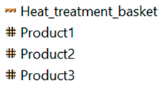
The material flow system is mapped using the position, size and length data determined on the basis of the on-site survey and the objects listed in Table 8.
- VII.
- Designing the information flow system: When preparing and running the simulation model, the following data structures and data input options must be provided:
- 1.
- Material handling machine table: Contains the speed data of the material handling machines (data fields: object, speed).
- 2.
- Loading table: Contains the time of loading products into the heat treatment basket and from the heat treatment basket into the granule spreading equipment (data fields: object name, duration).
- 3.
- Training table: Contains the data required for training the neural network (data fields: product weight, product quantity, number of heat treatment baskets, production lead time).
- 4.
- Input data for source objects: For three objects, the type and quantity of the product to be manufactured and the production interval. For one object, the type of heat treatment basket, the quantity to be manufactured and the production interval.
- 5.
- Input data for station objects: For three forging machines, the operating times, changeover batch size and changeover times.
- 6.
- Parallel station object data: Storage capacity and operating time of shot-blasting equipment.
- 7.
- Global variables: The weight of three products, the quantity to be manufactured, the number of heat treatment baskets, the production lead time, and the status information of the shot-blasting equipment.
- 8.
- Shift calendar input data: Shift schedule and break data for forging machines.
- 9.
- Product object: Size and weight data.
- 10.
- Container object: Heat treatment basket size and capacity data.
- 11.
- Buffer object: Quantity of heat treatment baskets.
- 12.
- Experiment Manager object: Parameters of run variants (ranges, scales).
- 13.
- Neural network object: Training data and related parameter settings.
- VIII.
- Defining the operating algorithm: Based on steps VI and VII, the operating algorithm comprises the following steps:
- 1.
- Setting initial parameters: Recording the data from steps VII. 1–2 and 4–12.
- 2.
- Generation of synthetic data: Use the Experiment Manager object to create run variants, then run them to generate synthetic data.
- 3.
- Processing of results: From the synthetic data obtained, select, for each product combination, the data set with the shortest production lead time and, among these, the smallest number of heat treatment baskets (Equation (10)) for training the neural network.
- 4.
- Training the neural network: Training the neural network based on the input (three product types and related production quantities) and output (number of heat treatment baskets, production lead time) data corresponding to the optimal data sets.
- 5.
- Application: Determining the optimal number of heat treatment baskets and production lead time for the product types and production quantities to be manufactured next week.
- IX.
- Determination of automatic data connection and system integration: Not relevant in this case.
- X.
- Definition of automatic feedback and intervention mechanisms: Not relevant in this case.
- XI.
- Recording data update and synchronisation principles: If the operation of the examined system changes (e.g., shift schedule, number of machines, characteristics), it becomes necessary to correct the model and retrain the neural network with new data. In the basic case, production plan data is recorded and examined on a weekly basis.
- XII.
- Recording cybersecurity and operational safety requirements: Not relevant for digital models.
- XIII.
- Defining system-level verification and validation principles: The three levels defined in Section 3 are applied with the following criteria: (i) simulation model verification—the model reproduces the predefined material flow structure and operating logic of the real system without errors; (ii) AI component validation—for ten random test cases, the production lead time obtained with the AI-determined optimal number of heat treatment baskets must not deviate by more than 5% from that determined by simulation; and (iii) integrated system validation—using ±5 heat treatment baskets relative to the optimum determined by the neural network must not improve the production lead time by more than 1%. Since the dimensions and operating parameters of the model are fictitious, operational validation against the historical data of the real system (e.g., comparing simulated and recorded production lead times) could not be performed; in an industrial implementation, this comparison should complement criteria (i)–(iii).
- XIV.
- Determination of model version and documentation requirements: All significant modifications are recorded as separate model versions with a unique identifier and date. The documentation covers the purpose, scope and main assumptions of the model, the operation of the simulation and AI components, the interpretation and ranges of the input and output variables, the verification and validation procedures and results, and the process of applying and modifying the model.
- 7.
- Implementation: Based on points I–XII of step 6, the simulation test model is created in the Plant Simulation framework (Figure 10).Figure 10. Simulation test model of a forging plant.
- 8.
- Testing and improving the test model: This step follows Step XIII. First, simulation model verification was performed by animation-based tracing of products and baskets along the planned route (forging, loading, heat treatment, shot-blasting), step-by-step tracking of individual units in the event log, material balance checks, extreme value tests with very low and very high numbers of baskets, and comparison with hand calculations for simple deterministic cases. As the case study uses modified data, no validation against historical data of the real system was performed. Second, AI component validation was performed as follows. With the help of the Experiment Manager object, 72,000 run variants were created based on Table 7, and 8000 optimal data sets were selected for training the neural network using the results of these runs. For each input combination, the run with the minimum production lead time and, in case of ties, with the smaller number of baskets was selected (Equation (10)). In the neural network module built into the Plant Simulation framework, the data in columns 1–6 of Table 7 represent the six neurons of the input layer, while the associated optimal heat treatment basket number and production lead time represent the two neurons of the output layer. The neural network contains two hidden layers with 10 neurons each. The network was trained with gradient-descent back-propagation, using a hyperbolic tangent (tanh) activation function, an activation magnitude of 0.9, a training data ratio of 90%, a re-initialization threshold of 1%, adaptive learning rates (Eta = 0.2–2.0), a momentum coefficient (Alpha) of 2 and an error batch size of 1 (Alpha (α = 2) is the momentum coefficient, scaling the previous weight update. It is applied conditionally within the built-in training algorithm, which combines backpropagation with Quickpropagation and adaptive learning rates). These values are reported exactly as specified in the built-in Neural Network module of Siemens Tecnomatix Plant Simulation. The 8000 data records were divided into training (90%, 7200 records) and validation (10%, 800 records) subsets by the built-in module. Apart from specifying the input data and the number of hidden layers (two), neurons (10 per layer) and training cycles (100), the default module settings were not modified, as the aim was not to find the best-performing neural network but to demonstrate the operating concept of the proposed framework. For illustration, the production lead time predictions for the ten test cases presented below were compared with simple benchmark models trained on the same 8000 data records. The neural network (mean relative deviation: 1.84%) outperformed the mean value predictor (9.29%), linear regression (4.47%) and quadratic regression (2.22%), whereas a k-nearest-neighbour model (k = 5) achieved a lower deviation (0.62%); these values are not directly comparable with the best mean error (3.32%) reported by the built-in neural network module, which refers to the training and validation records and both output variables rather than to the ten test cases. This indicates that other methods may be more accurate and that selecting the AI method (Step IV) is a genuine design decision within the method-agnostic framework. The accuracy of the neural network could also be improved by adjusting its structure, activation function, learning parameters and number of training cycles; identifying better-performing configurations remains a subject for future research. As the module version used did not allow user-defined random seeds or multiple independent training restarts, the network was trained in a single run with the default implementation. Instead of applying an early stopping criterion, the built-in neural network module automatically re-initializes the network when no significant improvement of the error is achieved, thereby reducing the risk of convergence to a local minimum. After 100 training cycles (the module’s default setting), the built-in neural network module reported a best mean error of 3.32%, defined as the lowest mean absolute relative error across the training and validation records and both output variables. The neural network was not intended to replace the simulation-based optimisation but to approximate the relationship between the process parameters and the corresponding optimal simulation outputs, enabling rapid prediction of the optimal number of heat treatment baskets and the production lead time without repeated discrete-event simulation runs.
To evaluate the neural network, ten input data sets were defined after training (Table 9), and their outputs were generated by the neural network. As they were not included in the training dataset, they represent previously unseen (out-of-sample) test cases.
Table 9.
Result data determined by the neural network.
Finally, integrated system validation was performed by comparing the AI-predicted optimal number of heat treatment baskets with the corresponding results obtained from the simulation model. Since the number of baskets is a discrete decision variable in the simulation model, the continuous predictions of all ten test cases (Table 9) were rounded up to the next integer before the validation runs (Table 10); for example, the predicted values of 61.94, 67.19 and 70.96 in Calculations 1–3 were implemented as 62, 68 and 71 heat treatment baskets, respectively. The corresponding rounding adjustments ranged from +0.04 to +0.81 baskets, corresponding to relative deviations (see below) between 0.06% and 1.21%. The robustness of the AI-supported decision was examined by simulating a ±5 basket deviation from the predicted optimum (Table 10). The lead times predicted by the neural network (Table 9) deviated from the simulated values by 0.13–4.27% (mean: 1.84%), i.e., below the 5% threshold in all ten cases; the neural network underestimated the lead time in Calculations 1–5, 7 and 8 and overestimated it in Calculations 6, 9 and 10. Reducing the number of baskets by five increased the production lead time in all ten cases (by 0.05–2.76%). Increasing the number of baskets by five did not change the lead time in Calculations 1, 2, 4, 7 and 9, increased it marginally in Calculations 3 and 10 (by 59 s and 1 s, respectively), and reduced it only slightly in Calculations 5, 6 and 8 (by at most 0.44%, in Calculation 5); thus, the achievable improvement remained below the 1% criterion in every case. These results suggest that, for the ten test cases, the neural network identified near-optimal solutions and that, above the predicted optimum, the lead time was practically insensitive to the number of baskets. This observation is specific to the analysed production conditions and should not be interpreted as a generally applicable decision rule.
Table 10.
Validation test results (Δ: change in production lead time relative to the predicted optimum).
The rounding of the continuous estimate to an integer value and the resulting relative deviation are formally:
where is the (continuous) number of baskets estimated by the neural network, nr is the integer value applied in the validation simulation, ⌈·⌉ denotes rounding up to the nearest integer (ceiling function), and δ is the relative deviation resulting from rounding (0.10%, 1.21%, 0.06%, 0.87%, 0.86%, 0.12%, 0.86%, 0.21%, 0.81% and 0.25% in Calculations 1–10, respectively).
The testing activities did not require any modifications to the simulation model developed during the design phase. The limitations arising from the single case study and the small number of out-of-sample test cases are discussed in Section 5.4.
- 9.
- Application of the simulation test system: The simulation test model is applied as specified in Step XIV. Based on the weekly production forecast plan, the optimal number of heat treatment baskets and the estimated production lead time are determined.
Further development of the simulation test model towards a digital shadow and digital twin concept:
- −
- Digital shadow: The parameters of the material handling machines and technological equipment in the test model are automatically updated based on the actual system’s operating data from the previous week. Using the updated parameter set, synthetic training data is generated for the neural network and the model is trained in an automated manner, which is expected to improve the accuracy of the optimisation results. For example, if the weekly production plan changes from 7000 to 9000 products with a heavier product mix, the updated data are transferred automatically from the ERP/MES system, and the model regenerates the training data, retrains the neural network and determines the updated optimal number of baskets for the following week. To implement the digital shadow, a unidirectional data connection between the company systems and the simulation model must be developed, along with principles for data cleaning and validation. It is also necessary to specify which model parameters are updated and how often the neural network is retrained. In addition, the output formats of decision support and the verification and validation procedures related to the updated model must be clearly defined.
- −
- Digital twin: The digital shadow concept is complemented by the automatic transfer and optimisation of the production plan. As a result of the optimisation, the number of heat treatment baskets determined is provided directly to the operating system via an automated system, thus creating a closed control loop between the digital model and the physical system. For instance, assume that one of the three forging machines becomes unavailable because of an unexpected breakdown. The digital twin automatically receives this information from the production control system, recalculates the optimal number of heat treatment baskets and the expected production lead time, and transmits the updated basket allocation directly to the production planning system. In this way, basket allocation can be adapted to the changed operating conditions without manual intervention.
5. Discussion
5.1. Positioning of the Framework Relative to Existing Approaches
The literature review showed that the integration of simulation and AI is typically reported for a specific function, such as synthetic data generation for AI training [8,32], simulation-based parameter optimisation using AI and metaheuristic techniques [30,31], reinforcement learning- and machine learning-based control [3,35,36] or hybrid simulation-based decision support [19,32], while digital maturity concepts are mostly used to classify or assess existing solutions [13,17,23,40]; approaches that support the application-specific improvement or investment appraisal of digital twins address a single solution rather than the choice between maturity levels for a given task [45,46]. The proposed framework differs from these approaches in three respects. First, it treats the digital maturity level as an explicit design decision taken before model development, rather than as a descriptive property of an already implemented solution. Second, it combines a rule-based preselection (Equations (8) and (9)) with a quantitative economic criterion (Equations (5)–(7)), so that the choice between digital model, digital shadow and digital twin can be justified both technically and economically. Third, it positions AI as an algorithm-independent functional capability (model selection, data preparation, prediction, optimisation, validation and decision support) that is assigned to well-defined development steps and intervention points of the simulation model. In this sense, the framework is complementary to the cited application-specific studies: they provide methods that can be inserted into steps IV and V of the framework, whereas the framework provides the procedural context in which these methods are selected, implemented, verified and operated.
Beyond the application-specific studies, the framework should also be positioned against established reference frameworks that address parts of the same problem (Table 11). The classification of Kritzinger et al. [13] distinguishes digital models, digital shadows and digital twins according to the degree of automation of the data flow between the physical and the digital object. Industry 4.0 maturity models, such as the model of Schumacher et al. [40] and the acatech Industrie 4.0 Maturity Index [23], assess the Industry 4.0 readiness and maturity of an entire organisation across several dimensions and, in the case of the acatech index, support the derivation of a transformation roadmap and recommend that the target stage be set according to company strategy and cost–benefit considerations rather than by default at the highest stage. However, they do not specify which digital maturity level should be implemented for an individual logistics process development task; it should be noted that, in the proposed framework, the term maturity is used in a narrower, solution-level sense, referring to the digital model, digital shadow and digital twin. At the level of individual digital twins, the maturity model of Uhlenkamp et al. [45] supports the application-specific evaluation and improvement of a given digital twin in production and logistics, and the report of Thomas [46] proposes a stepwise investment analysis for digital twins; however, neither compares the digital model, digital shadow and digital twin as mutually exclusive alternatives for the same logistics task or restricts the comparison to technically feasible types. CRISP-DM [41] structures data-mining projects from business understanding to deployment; however, it is oriented towards the analysis of available data and does not address the design of simulation models or the generation of synthetic training data by simulation. Its step-by-step guide includes a project-level cost–benefit analysis covering data collection, development, implementation and operating costs as well as the expected benefits [47]; these categories partly overlap with the CF, CA and CO terms of Equation (6), whereas the NLCC additionally discounts them over the evaluation period, compares alternative maturity levels and estimates the benefits as expected avoided losses (Equation (5)). The simulation study procedure of Banks et al. [42] and the verification and validation approach of Sargent [43] provide a mature basis for building and validating simulation models, but they do not consider AI components, data connections to the physical system or the selection of the digital maturity level.
Table 11.
Comparison of the proposed framework with established reference frameworks.
The novelty of the proposed framework is therefore integrative: for logistics process development, it organises the selection of the digital maturity level, simulation modelling, the application of AI and economic evaluation into a single, step-by-step methodology, building on the existing frameworks rather than replacing them. Its added value lies in the interfaces that remain undefined when the frameworks are applied separately. First, the digital maturity level is selected at the outset of the logistics development task; since this decision determines the data sources, integration requirements and costs of all subsequent steps, making it early may reduce the risk of costly redesign. Second, when the simulation model of the logistics process generates the training data for the AI component, the framework treats data preparation in the sense of CRISP-DM [41] and the experimental design of the simulation as a single coordinated activity (steps V–VIII). Third, the three-level V&V scheme of step XIII also provides for the validation of the combined simulation–AI system, which is not explicitly addressed by the classical simulation approaches [42,43] and is covered by CRISP-DM [41] only in the form of evaluating the data mining model against the business objectives. In this way, decisions that often depend on experience can be made more explicit and reproducible. Whether this leads to better project outcomes than the separate use of the existing methodologies remains to be confirmed in comparative studies across multiple industrial applications (Section 5.4).
5.2. Theoretical Implications
From a theoretical perspective, the study connects three strands of research that are usually discussed separately: the sequence of simulation studies, digital twin maturity models and AI-based decision support. The formal description of the three task types (Equations (1)–(4)) allows defining operational characteristics, selecting the ideal system variant and determining optimal parameters to be expressed not as independent problem classes, but as different uses of the same simulation mapping. This provides a common basis for linking simulation outputs with multi-criteria decision-making and optimisation. Furthermore, the NLCC criterion reframes the adoption of digital shadows and digital twins as an investment decision: provided that the lower level is technically feasible, a higher maturity level is justified only if the present value of its additional expected avoided losses outweighs the present value of the additional costs of data connectivity, feedback mechanisms and operation. This view counterbalances technology-driven expectations that a higher maturity level is inherently preferable.
5.3. Practical Implications
For practitioners, the framework may offer a structured sequence of decisions for industrial projects. The case study illustrates that a digital model may be the economically most favourable solution for periodic, offline planning tasks, even when digital shadow and digital twin solutions are technically feasible. At the same time, the framework indicates conditions under which an upgrade may become justified, for example when decisions must be made more frequently or when changes in system parameters must be reflected automatically, as outlined for the digital shadow and digital twin extensions of the case study.
The case study also suggests why simulation can be useful for such decisions: the production lead time saturated as the number of baskets increased, which is difficult to capture with simple rules of thumb; this supports both the lexicographic formulation of the task, in particular its ε-tolerant variant (Equation (10)) and the use of simulation-generated data for training the AI component. Finally, the detailed design steps (steps I–XIV) may serve as a checklist to help reduce the risk of omitting data, integration or validation requirements, which would otherwise only become apparent during implementation.
5.4. Generalisability of the Results
The framework was demonstrated through a single case study at the digital model level, using fictitious data and illustrative cost values. The simulation model was not validated against historical data of the real system; the reported validation covers the model logic and the agreement between the neural network and the simulation. Its general applicability, in particular the NLCC-based selection between maturity levels, therefore needs to be confirmed in further industrial applications with real cost data, preferably including digital shadow or digital twin implementations. The results should therefore be regarded as an illustration of the framework rather than as evidence of its general effectiveness. In addition, the AI component was evaluated on only ten out-of-sample test cases, the neural network was trained in a single run with largely default settings, and a simple k-nearest-neighbour benchmark achieved a lower deviation; the case study therefore does not indicate which AI method is most suitable for the task. Furthermore, the literature review was based on a purposive selection of 48 publications retrieved with umbrella search terms, so relevant studies using more specific terminology may have been missed. Because the framework is method-agnostic with respect to the AI component, its structure does not depend on the predictive performance of the neural network used in the case study; however, the performance of different AI methods within the framework remains a subject for future research.
6. Conclusions
This study developed an integrated methodological framework for logistics process development that combines simulation modelling, artificial intelligence (AI), digital maturity selection and economic evaluation within a unified development lifecycle. Based on a structured literature review of 48 selected publications, two principal methodological gaps were identified: the lack of a comprehensive process development framework integrating simulation and AI, and the absence of explicit technical and economic guidance for selecting between digital models, digital shadows and digital twins.
The first major result is a four-phase, step-by-step methodology covering problem formulation, simulation and AI model design, implementation and validation, and operational application. The framework accommodates three fundamental process development objectives: determining operational characteristics, selecting the preferred system alternative and optimising operating parameters. It also defines algorithm-independent AI functions and their roles within the development process, allowing different AI techniques to be integrated according to the requirements of the task.
The second major result is a decision procedure for selecting the appropriate digital maturity level. The proposed approach combines rule-based technical feasibility assessment with discounted net life-cycle cost (NLCC) evaluation, considering implementation and operating costs alongside expected avoided losses. The illustrative economic assessment identified the digital model as the most favourable alternative for the examined planning task, demonstrating that higher digital maturity is not necessarily economically justified.
The third major result is the demonstration of the proposed framework through an industry-inspired logistics process development case study. Simulation was used to determine optimal operating parameters, while a neural network trained on simulation-generated data supported their prediction under different operating conditions.
Overall, the proposed approach provides a structured basis for selecting and applying digital technologies according to the requirements of individual logistics process development tasks, rather than assuming that higher technological maturity necessarily leads to better outcomes. Although the case study demonstrates the applicability of the framework at the digital model level, further industrial applications using real operational and economic data would allow its broader applicability and practical benefits to be evaluated.
Funding
This research was supported by the János Bolyai Research Scholarship of the Hungarian Academy of Sciences. Project No. 2023-1.2.4-TÉT-2023-00027 has been implemented with the support provided by the Ministry of Culture and Innovation of Hungary from the National Research, Development and Innovation Fund, and was financed under the 2023-1.2.4-TÉT funding scheme.
Institutional Review Board Statement
Not applicable.
Informed Consent Statement
Not applicable.
Data Availability Statement
The datasets generated and analysed during the current study are available from the corresponding author upon reasonable request.
Acknowledgments
During the preparation of this manuscript, the author used ChatGPT (GPT-6, OpenAI) for the purposes of improving language clarity and stylistic quality. The author has reviewed and edited the output and takes full responsibility for the content of this publication.
Conflicts of Interest
The author declares no conflicts of interest.
References
- Rane, N.L.; Desai, P.; Rane, J.; Paramesha, M. Artificial Intelligence, Machine Learning, and Deep Learning for Sustainable and Resilient Supply Chain and Logistics Management. In Trustworthy Artificial Intelligence in Industry and Society; Deep Science Publishing: London, UK, 2024; pp. 156–184. [Google Scholar] [CrossRef] [Scilit] [PubMed]
- Tamás, P. New Dimensions in the Study of Outsourcing Logistics Services: The Role of Digitalization in Enhancing Efficiency. Logistics 2025, 9, 44. [Google Scholar] [CrossRef] [Scilit]
- Biller, B.; Biller, S. Implementing Digital Twins That Learn: AI and Simulation Are at the Core. Machines 2023, 11, 425. [Google Scholar] [CrossRef] [Scilit]
- Jackson, I.; Saenz, M.J.; Ivanov, D. From Natural Language to Simulations: Applying AI to Automate Simulation Modelling of Logistics Systems. Int. J. Prod. Res. 2024, 62, 1434–1457. [Google Scholar] [CrossRef] [Scilit]
- Chen, W.; Men, Y.; Fuster, N.; Osorio, C.; Juan, A.A. Artificial Intelligence in Logistics Optimization with Sustainable Criteria: A Review. Sustainability 2024, 16, 9145. [Google Scholar] [CrossRef] [Scilit]
- Rodríguez Rodríguez, C.B.; Galpert Cañizares, D.R.; Knudsen González, J.A.; Silva Delgado, A.V.; Hernández Pérez, G.D. Artificial Intelligence Contribution to the Development of Cuban Port Logistics Chains. In Computational Intelligence in Engineering and Project Management; Studies in Computational Intelligence; Springer: Cham, Switzerland, 2024; Volume 1134, pp. 257–273. [Google Scholar] [CrossRef] [Scilit]
- Berti, N.; Finco, S. Digital Twin and Human Factors in Manufacturing and Logistics Systems: State of the Art and Future Research Directions. IFAC-PapersOnLine 2022, 55, 1893–1898. [Google Scholar] [CrossRef] [Scilit]
- Minbashi, N.; Zhao, J.; Dick, C.T.; Bohlin, M. Enhancing Freight Train Delay Prediction with Simulation-Assisted Machine Learning. IET Intell. Transp. Syst. 2024, 18, 2359–2374. [Google Scholar] [CrossRef] [Scilit]
- Snyder, H. Literature Review as a Research Methodology: An Overview and Guidelines. J. Bus. Res. 2019, 104, 333–339. [Google Scholar] [CrossRef] [Scilit]
- van Eck, N.J.; Waltman, L. Software Survey: VOSviewer, a Computer Program for Bibliometric Mapping. Scientometrics 2010, 84, 523–538. [Google Scholar] [CrossRef] [Scilit] [PubMed]
- Haddaway, N.R.; Collins, A.M.; Coughlin, D.; Kirk, S. The Role of Google Scholar in Evidence Reviews and Its Applicability to Grey Literature Searching. PLoS ONE 2015, 10, e0138237. [Google Scholar] [CrossRef] [Scilit] [PubMed]
- Cselényi, J.; Illés, B. (Eds.) Anyagáramlási Rendszerek Tervezése és Irányítása I (Material Flow Systems Design and Control I); Miskolci Egyetemi Kiadó: Miskolc, Hungary, 2006; ISBN 963-661-672-8. [Google Scholar]
- Kritzinger, W.; Karner, M.; Traar, G.; Henjes, J.; Sihn, W. Digital Twin in Manufacturing: A Categorical Literature Review and Classification. IFAC-PapersOnLine 2018, 51, 1016–1022. [Google Scholar] [CrossRef] [Scilit]
- Kosasih, E.E.; Brintrup, A. Reinforcement Learning Provides a Flexible Approach for Realistic Supply Chain Safety Stock Optimisation. IFAC-PapersOnLine 2022, 55, 1539–1544. [Google Scholar] [CrossRef] [Scilit]
- Kłosowski, G.; Gola, A.; Thibbotuwawa, A. Computational Intelligence in Control of AGV Multimodal Systems. IFAC-PapersOnLine 2018, 51, 1421–1427. [Google Scholar] [CrossRef] [Scilit]
- Dereli, T.; Daş, G.S. Development of a Decision Support System for Solving Container Loading Problems. Transport 2010, 25, 138–147. [Google Scholar] [CrossRef] [Scilit]
- Tamás, P. Integration Possibilities of Logistics Process Simulation and VR Technology. Teh. Glas. 2025, 19, 82–87. [Google Scholar] [CrossRef] [Scilit]
- Woschank, M.; Rauch, E.; Zsifkovits, H. A Review of Further Directions for Artificial Intelligence, Machine Learning, and Deep Learning in Smart Logistics. Sustainability 2020, 12, 3760. [Google Scholar] [CrossRef] [Scilit]
- Shadkam, E.; Irannezhad, E. A Comprehensive Review of Simulation Optimization Methods in Agricultural Supply Chains and Transition towards an Agent-Based Intelligent Digital Framework for Agriculture 4.0. Eng. Appl. Artif. Intell. 2025, 143, 109930. [Google Scholar] [CrossRef] [Scilit]
- Long, P.; Lu, L.; Chen, Q.; Chen, Y.; Li, C.; Luo, X. Intelligent Selection of Healthcare Supply Chain Mode—An Applied Research Based on Artificial Intelligence. Front. Public Health 2023, 11, 1310016. [Google Scholar] [CrossRef] [Scilit] [PubMed]
- Zeng, Y.Q.; Li, W.B.; Li, C.H. A Dynamic Simulation Framework Based on Hybrid Modeling Paradigm for Parallel Scheduling Systems in Warehouses. Simul. Model. Pract. Theory 2024, 133, 102921. [Google Scholar] [CrossRef] [Scilit]
- Osman, R.; El-Gendy, S. Interconnected and Resilient: A CGE Analysis of AI-Driven Cyberattacks in Global Trade. Risk Anal. 2025, 45, 846–862. [Google Scholar] [CrossRef] [Scilit] [PubMed]
- Schuh, G.; Anderl, R.; Dumitrescu, R.; Krüger, A.; ten Hompel, M. (Eds.) Industrie 4.0 Maturity Index: Managing the Digital Transformation of Companies—Update 2020; acatech STUDY; acatech—National Academy of Science and Engineering: Munich, Germany, 2020. [Google Scholar]
- Didast, F.Z.; Nassih, R.; Ait Elbachir, I. Artificial Intelligence and Logistics: Recent Trends and Development. Preprints 2024, 2024102141. [Google Scholar] [CrossRef] [Scilit]
- Hermans, M.; Tamás, P. Applying Bayesian Neural Networks to Optimize Maintenance Logistics. Acta Logist. 2026, 13, 162–173. [Google Scholar] [CrossRef] [Scilit]
- du Plessis, M.J.; Gerber, R.; Goedhals-Gerber, L.L.; van Eeden, J. Shaping the Future of Freight Logistics: Use Cases of Artificial Intelligence. Sustainability 2025, 17, 1355. [Google Scholar] [CrossRef] [Scilit]
- Bui, H.P.; Tran, T.H.; Nguyen, L.D.; Vu, T.Y.C.; Pham, B.; Can, T.Y.; Le, T.G. Applications of Artificial Intelligence (AI) in the Logistics Industry in Vietnam: Opportunities and Challenges. Int. J. Sci. Res. Methodol. 2025, 13, 2202–2207. [Google Scholar] [CrossRef] [Scilit]
- Fang, B.; Yu, J.; Chen, Z.; Osman, A.I.; Farghali, M.; Ihara, I.; Hamza, E.H.; Rooney, D.W.; Yap, P.S. Artificial Intelligence for Waste Management in Smart Cities: A Review. Environ. Chem. Lett. 2023, 21, 1959–1989. [Google Scholar] [CrossRef] [Scilit] [PubMed]
- Carreira-Munich, T.; Paz-Marcolla, V.; Castro, R. DEVS Copilot: Towards Generative AI-Assisted Formal Simulation Modeling Based on Large Language Models. In Proceedings of the 2024 Winter Simulation Conference (WSC), Orlando, FL, USA, 15–18 December 2024; pp. 2785–2796. [Google Scholar] [CrossRef] [Scilit]
- Boru, A.; Dosdoğru, A.T.; Göçken, M.; Erol, R. A Novel Hybrid Artificial Intelligence Based Methodology for the Inventory Routing Problem. Symmetry 2019, 11, 717. [Google Scholar] [CrossRef] [Scilit]
- Amaran, S.; Sahinidis, N.V.; Sharda, B.; Bury, S.J. Simulation Optimization: A Review of Algorithms and Applications. Ann. Oper. Res. 2016, 240, 351–380. [Google Scholar] [CrossRef] [Scilit]
- von Rueden, L.; Mayer, S.; Sifa, R.; Bauckhage, C.; Garcke, J. Combining Machine Learning and Simulation to a Hybrid Modelling Approach: Current and Future Directions. In Advances in Intelligent Data Analysis XVIII; Berthold, M.R., Feelders, A., Krempl, G., Eds.; Lecture Notes in Computer Science; Springer: Cham, Switzerland, 2020; Volume 12080, pp. 548–560. [Google Scholar] [CrossRef] [Scilit]
- Ivanov, D. Intelligent Digital Twin (iDT) for Supply Chain Stress-Testing, Resilience, and Viability. Int. J. Prod. Econ. 2023, 263, 108938. [Google Scholar] [CrossRef] [Scilit]
- Ivanov, D. Conceptual and Formal Models for Design, Adaptation, and Control of Digital Twins in Supply Chain Ecosystems. Omega 2025, 137, 103356. [Google Scholar] [CrossRef] [Scilit]
- da Silva, M.R.F.; Agostino, I.R.S.; Frazzon, E.M. Integration of Machine Learning and Simulation for Dynamic Rescheduling in Truck Appointment Systems. Simul. Model. Pract. Theory 2023, 125, 102747. [Google Scholar] [CrossRef] [Scilit]
- Rolf, B.; Jackson, I.; Müller, M.; Lang, S.; Reggelin, T.; Ivanov, D. A Review on Reinforcement Learning Algorithms and Applications in Supply Chain Management. Int. J. Prod. Res. 2023, 61, 7151–7179. [Google Scholar] [CrossRef] [Scilit]
- Zhang, M.; Grosse, E.H.; Glock, C.H. Ergonomic and Economic Evaluation of a Collaborative Hybrid Order Picking System. Int. J. Prod. Econ. 2023, 258, 108774. [Google Scholar] [CrossRef] [Scilit]
- Min, K.J.; Chung, B.D.; Cho, G.S. Agent-Based Modelling for Human–Robot Collaborative Order Picking System Considering Workers’ Performance. Int. J. Prod. Res. 2025, 63, 4934–4957. [Google Scholar] [CrossRef] [Scilit]
- Olan, F.; Spanaki, K.; Ahmed, W.; Zhao, G. Enabling Explainable Artificial Intelligence Capabilities in Supply Chain Decision Support Making. Prod. Plan. Control 2025, 36, 808–819. [Google Scholar] [CrossRef] [Scilit]
- Schumacher, A.; Erol, S.; Sihn, W. A Maturity Model for Assessing Industry 4.0 Readiness and Maturity of Manufacturing Enterprises. Procedia CIRP 2016, 52, 161–166. [Google Scholar] [CrossRef] [Scilit]
- Wirth, R.; Hipp, J. CRISP-DM: Towards a Standard Process Model for Data Mining. In Proceedings of the 4th International Conference on the Practical Applications of Knowledge Discovery and Data Mining, Manchester, UK, 11–13 April 2000; pp. 29–39. [Google Scholar]
- Banks, J.; Carson, J.S., II; Nelson, B.L.; Nicol, D.M. Discrete-Event System Simulation, 5th ed.; Pearson: Upper Saddle River, NJ, USA, 2010. [Google Scholar]
- Sargent, R.G. Verification and Validation of Simulation Models. J. Simul. 2013, 7, 12–24. [Google Scholar] [CrossRef] [Scilit]
- Smalley, A. Four Types of Problems: From Reactive Troubleshooting to Creative Innovation; Lean Enterprise Institute: Cambridge, MA, USA, 2018. [Google Scholar]
- Uhlenkamp, J.-F.; Baalsrud Hauge, J.; Broda, E.; Lütjen, M.; Freitag, M.; Thoben, K.-D. Digital Twins: A Maturity Model for Their Classification and Evaluation. IEEE Access 2022, 10, 69605–69635. [Google Scholar] [CrossRef] [Scilit]
- Thomas, D. Economics of Digital Twins: Costs, Benefits, and Economic Decision Making; NIST Advanced Manufacturing Series 100-61; National Institute of Standards and Technology: Gaithersburg, MD, USA, 2024. [Google Scholar] [CrossRef] [Scilit]
- Chapman, P.; Clinton, J.; Kerber, R.; Khabaza, T.; Reinartz, T.; Shearer, C.; Wirth, R. CRISP-DM 1.0: Step-by-Step Data Mining Guide; SPSS Inc.: Chicago, IL, USA, 2000. [Google Scholar]
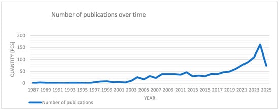
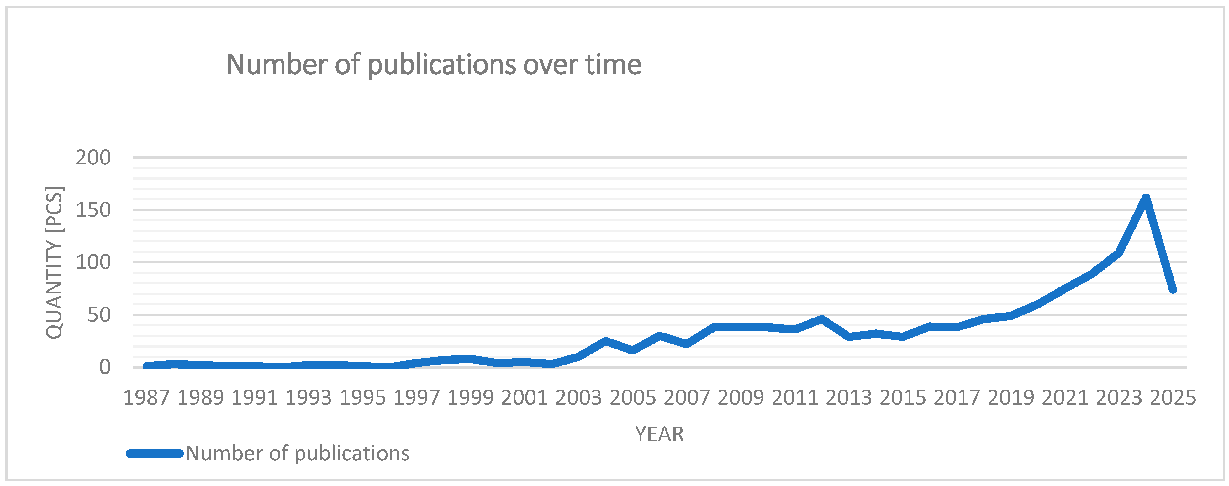
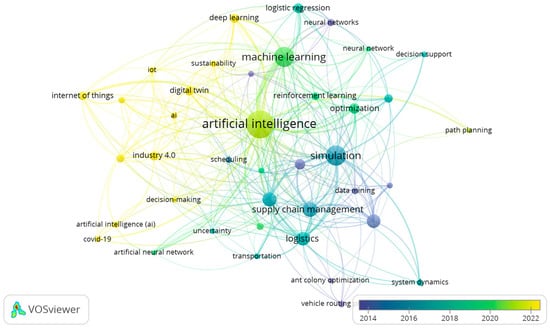
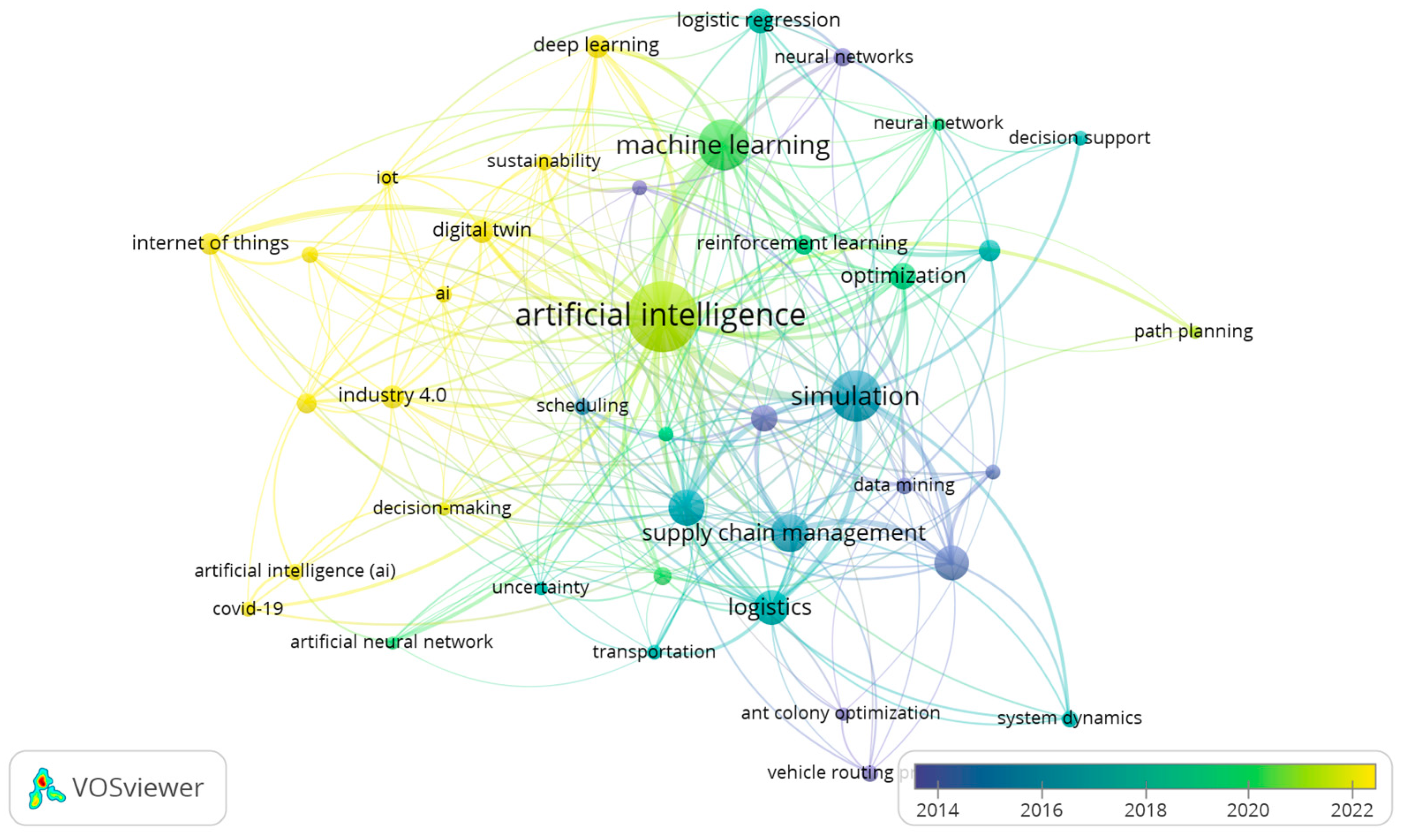
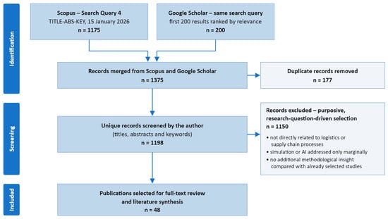
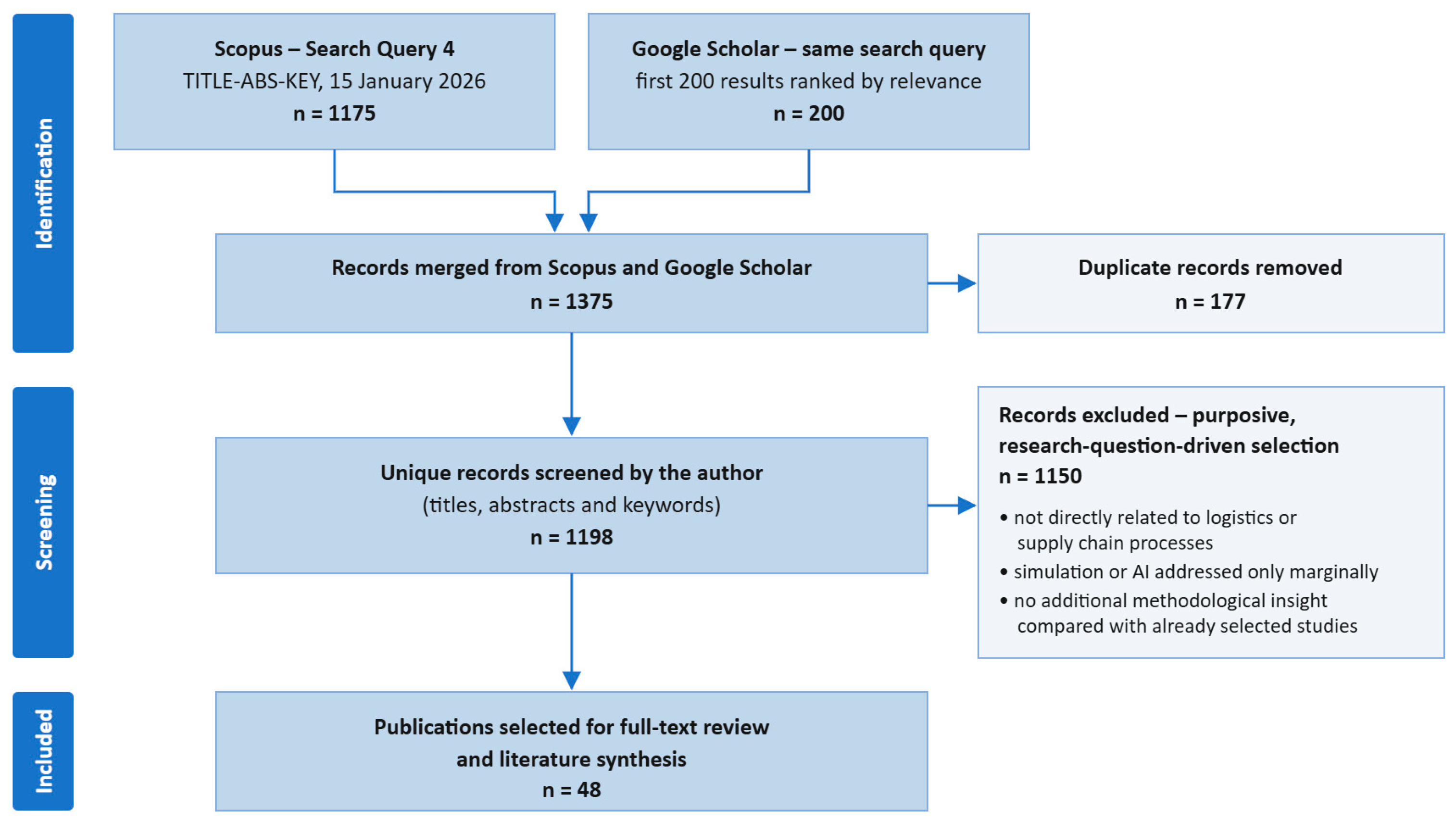
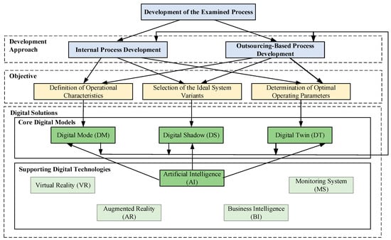
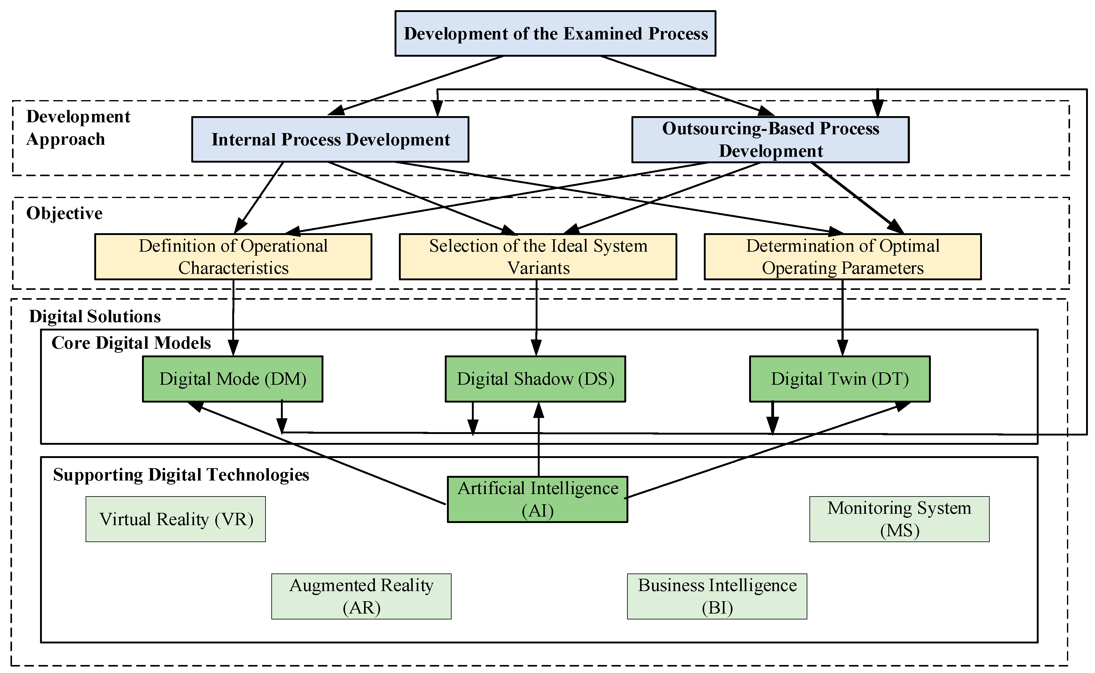
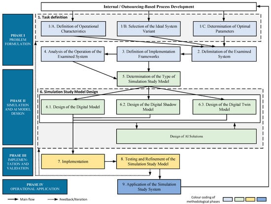
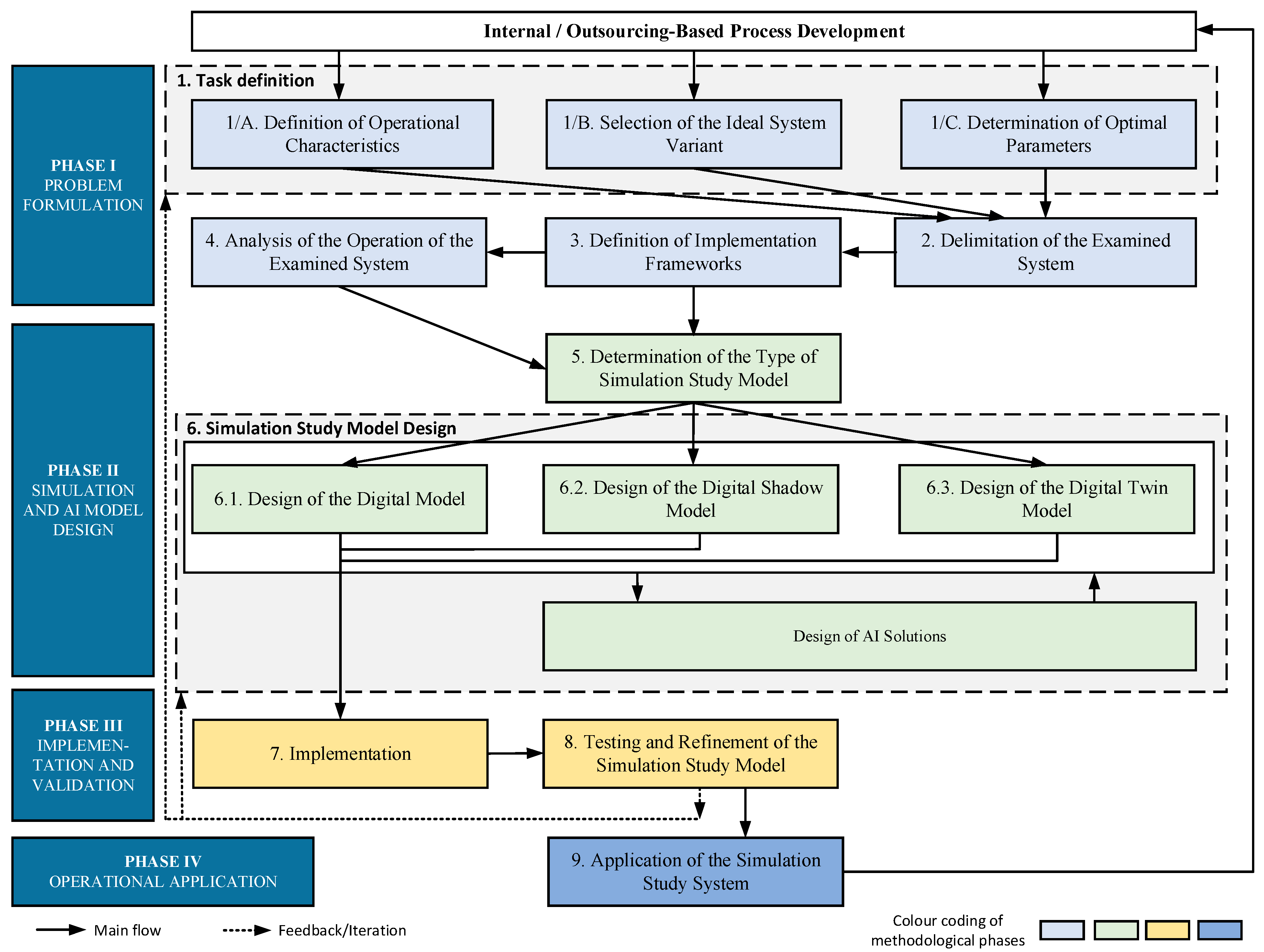
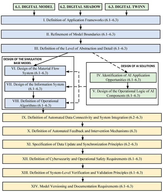
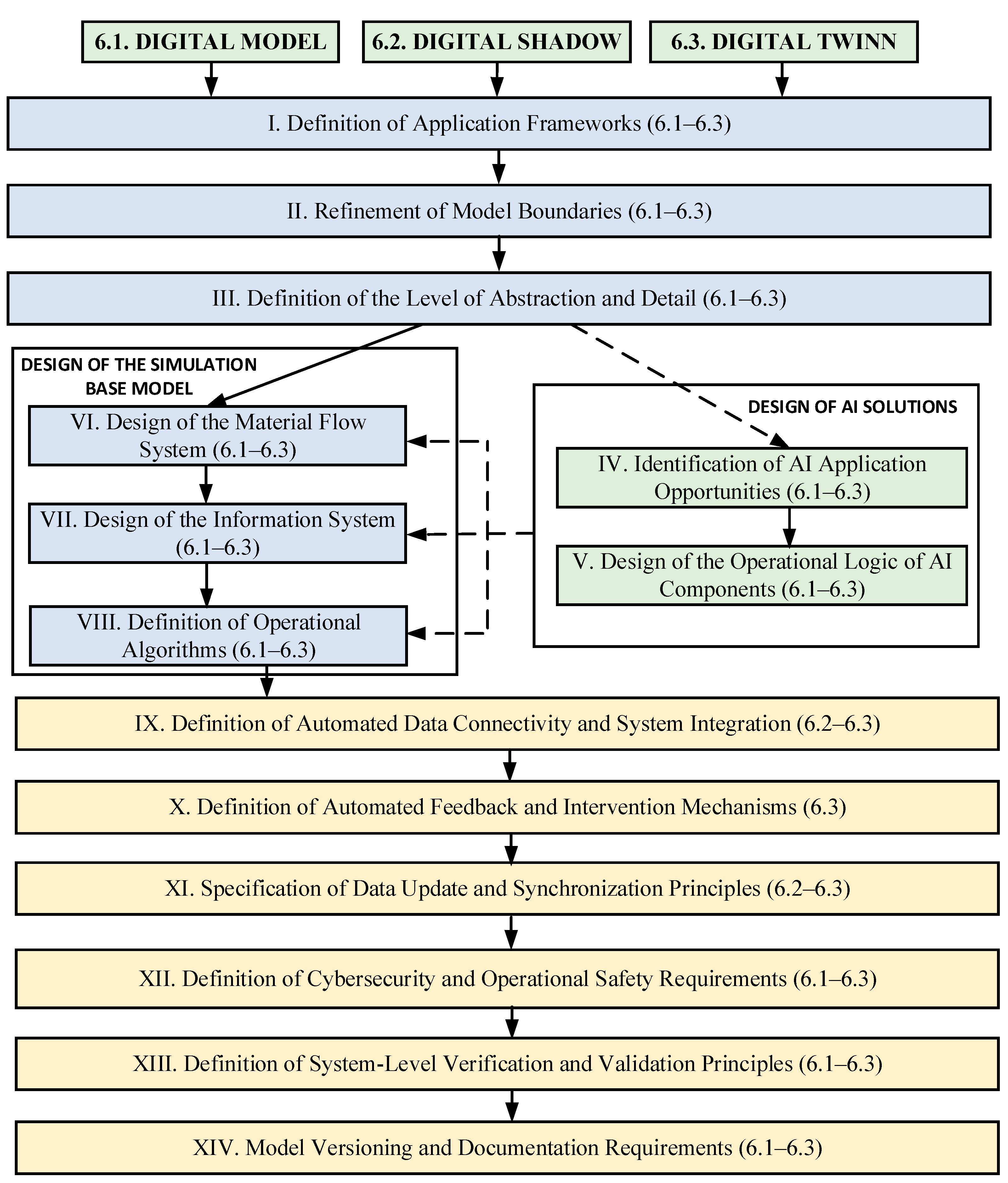
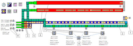
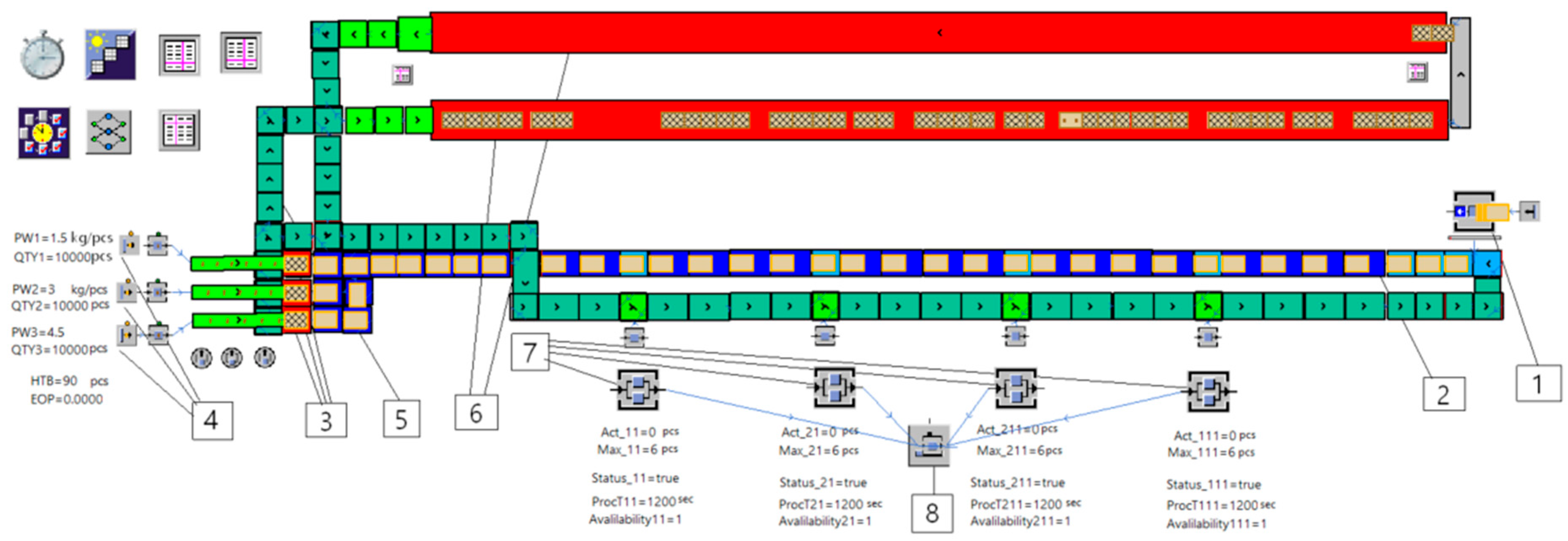
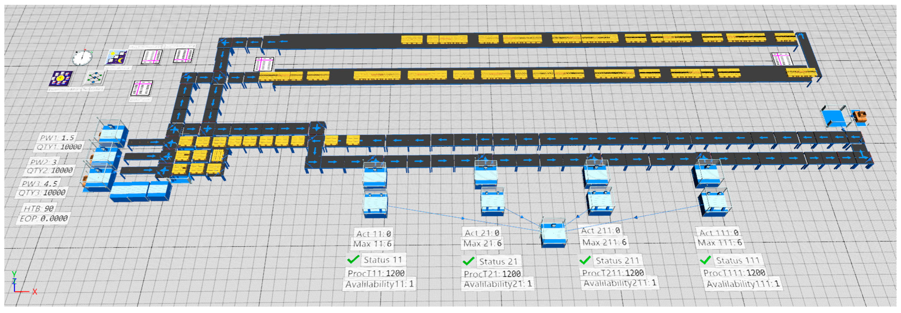

Disclaimer/Publisher’s Note: The statements, opinions and data contained in all publications are solely those of the individual author(s) and contributor(s) and not of MDPI and/or the editor(s). MDPI and/or the editor(s) disclaim responsibility for any injury to people or property resulting from any ideas, methods, instructions or products referred to in the content. |
© 2026 by the author. Licensee MDPI, Basel, Switzerland. This article is an open access article distributed under the terms and conditions of the Creative Commons Attribution (CC BY) license.