Integration of Partial Least Squares Regression and Hyperspectral Data Processing for the Nondestructive Detection of the Scaling Rate of Carp (Cyprinus carpio)


Abstract
1. Introduction
2. Materials and Methods
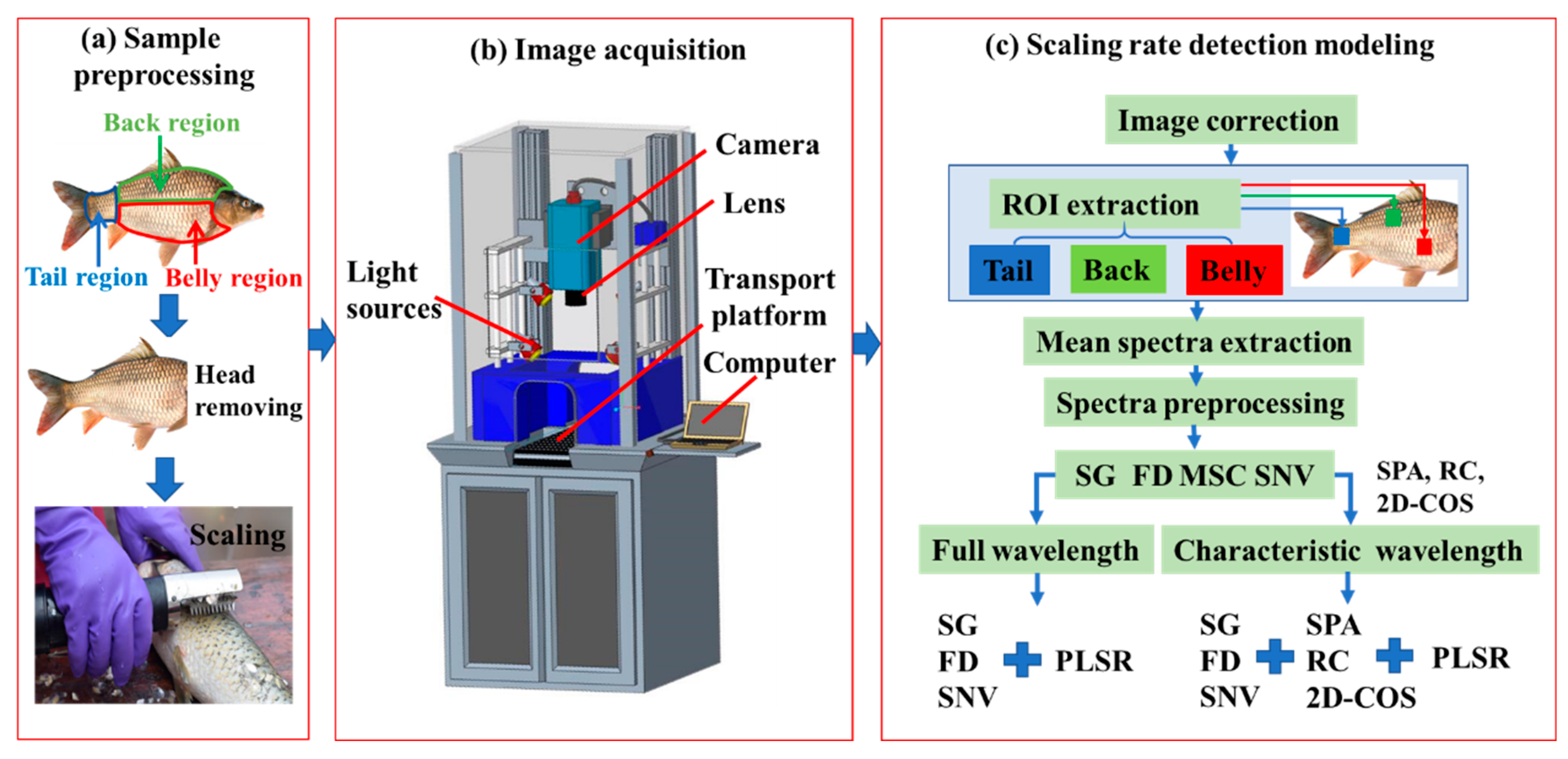
2.1. Preparation of Samples
2.2. Hyperspectral Imaging System
2.3. Correction of Spectra
2.4. Spectral Preprocessing
2.5. Selection of CWs
2.6. PLSR Scaling Rate Detection Model
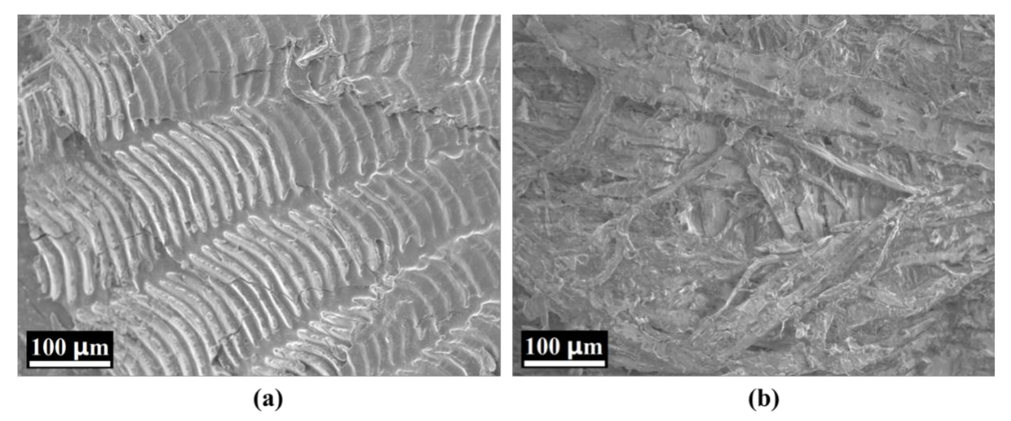
2.7. Scanning Electron Microscopy (SEM)
3. Results and Discussion
3.1. Data Analysis of Original Spectra
3.2. Spectral Preprocessing
3.3. Selection of CWs
3.3.1. SPA
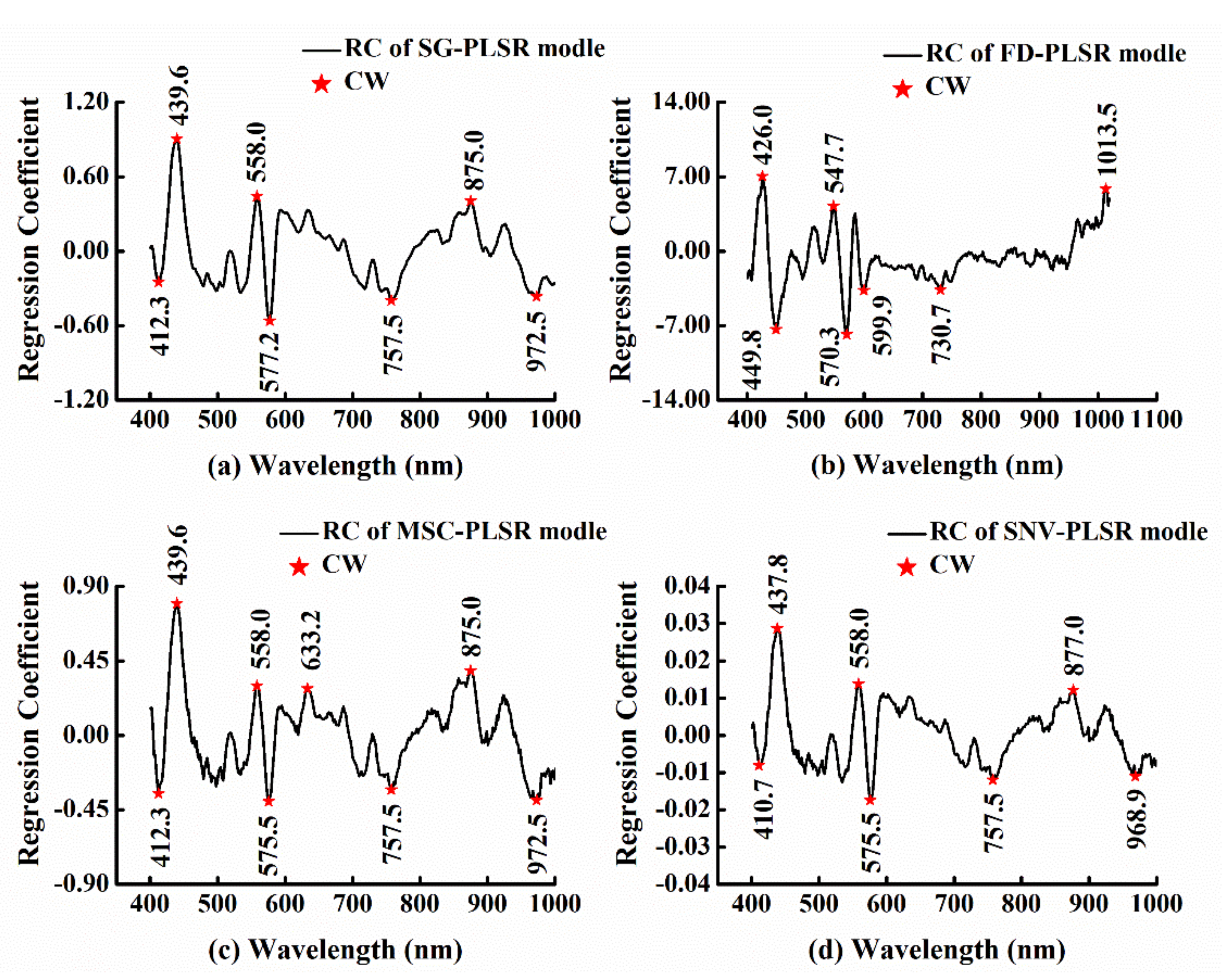
3.3.2. RC
3.3.3. 2D-COS
3.4. Analysis of the PLSR Scaling Rate Detection Model
3.4.1. Model of the Back Region
3.4.2. Model of the Belly Region
3.4.3. Model of the Tail Region
4. Conclusions
Author Contributions
Funding
Conflicts of Interest
References
- Jackman, P.; Sun, D.W.; Du, C.J.; Allen, P.; Downey, G. Prediction of beef eating quality from colour, marbling and wavelet texture features. Meat Sci. 2008, 80, 1273–1281. [Google Scholar] [CrossRef] [PubMed]
- Cubero, S.; Aleixos, N.; Moltó, E.; Gómez-Sanchis, J.; Blasco, J. Advances in Machine Vision Applications for Automatic Inspection and Quality Evaluation of Fruits and Vegetables. Food Biop. Technol. 2011, 4, 487–504. [Google Scholar] [CrossRef]
- Iqbal, S.M.; Gopal, A.; Sankaranarayanan, P.E.; Nair, A.B. Classification of Selected Citrus Fruits Based on Color Using Machine Vision System. Int. J. Food Prop. 2016, 19, 272–288. [Google Scholar] [CrossRef]
- Li, J.B.; Huang, W.Q.; Zhao, C.J. Machine vision technology for detecting the external defects of fruits—A review. Imaging Sci. J. 2015, 63, 241–251. [Google Scholar] [CrossRef]
- Su, Q.H.; Kondo, N.; Li, M.Z.; Sun, H.; Al Riza, D.F.; Habaragamuwa, H. Potato quality grading based on machine vision and 3D shape analysis. Comput. Electron. Agric. 2018, 152, 261–268. [Google Scholar] [CrossRef]
- Liu, D.; Zeng, X.A.; Sun, D.W. Recent Developments and Applications of Hyperspectral Imaging for Quality Evaluation of Agricultural Products: A Review. Crit. Rev. Food Sci. Nutr. 2015, 55, 1744–1757. [Google Scholar] [CrossRef]
- Lennon, M.; Mouchot, M.C.; Mercier, G.; Hubert-Moy, L. Segmentation of hedges on CASI hyperspectral images by data fusion from texture, spectral and shape analysis. In Proceedings of the Geoscience and Remote Sensing Symposium, IEEE 2000 International IGARSS 2000, Honolulu, HI, USA, 24–28 July 2000; pp. 825–827. [Google Scholar]
- Jiang, Y.L.; Zhang, R.Y.; Yu, J.; Hu, W.C.; Yin, Z.T. Detection of Infected Tephritidae Citrus Fruit Based on Hyperspectral Imaging and Two-Band Ratio Algorithm. Adv. Mater. Res. 2011, 311, 1501–1504. [Google Scholar] [CrossRef]
- Qiao, J.; Wang, N.; Ngadi, M.O.; Gunenc, A.M.; Prasher, S.O. Prediction of drip-loss, pH, and color for pork using a hyperspectral imaging technique. Meat Sci. 2007, 76, 1–8. [Google Scholar] [CrossRef]
- Zhao, J.; Vittayapadung, S.; Chen, Q.; Chaitep, S.; Chuaviroj, R. Nondestructive measurement of sugar content of apple using hyperspectral imaging technique. Maejo Int. J. Sci. Technol. 2009, 3, 130–142. [Google Scholar]
- Gila, D.M.M.; Marchal, P.C.; García, J.G.; Ortega, J.G. On-line system based on hyperspectral information to estimate acidity, moisture and peroxides in olive oil samples. Comput. Electron. Agric. 2015, 116, 1–7. [Google Scholar] [CrossRef]
- Wu, D.; Wang, S.; Wang, N.; Nie, P.; He, Y.; Sun, D.W.; Yao, J. Application of Time Series Hyperspectral Imaging (TS-HSI) for Determining Water Distribution Within Beef and Spectral Kinetic Analysis During Dehydration. Food Bioprocess Technol. 2013, 6, 2943–2958. [Google Scholar] [CrossRef]
- Manley, M.; Williams, P.; Nilsson, D.; Geladi, P. Near Infrared Hyperspectral Imaging for the Evaluation of Endosperm Texture in Whole Yellow Maize (Zea maize L.) Kernels. J. Agric. Food Chem. 2009, 57, 8761–8769. [Google Scholar] [CrossRef] [PubMed]
- Nicola, B.M.; Defraeye, T.; De Ketelaere, B.; Herremans, E.; Hertog, M.L.A.T.M.; Saeys, W.; Torricelli, A.; Vandendriessche, T.; Verboven, P. Nondestructive Measurement of Fruit and Vegetable Quality. Rev. Food Sci. Technol. 2014, 5, 285–312. [Google Scholar] [CrossRef] [PubMed]
- Zhu, F.; Zhang, D.; He, Y.; Liu, F.; Sun, D.W. Application of Visible and Near Infrared Hyperspectral Imaging to Differentiate Between Fresh and Frozen–Thawed Fish Fillets. Food. Bioprocess Technol. 2013, 6, 2931–2937. [Google Scholar] [CrossRef]
- Zhu, S.S.; Feng, L.; Zhang, C.; Bao, Y.D.; He, Y. Identifying Freshness of Spinach Leaves Stored at Different Temperatures Using Hyperspectral Imaging. Foods 2019, 8, E356. [Google Scholar] [CrossRef] [PubMed]
- Di, W.; Hui, S.; Yong, H.; Yu, X.; Bao, Y. Potential of hyperspectral imaging and multivariate analysis for rapid and non-invasive detection of gelatin adulteration in prawn. J. Food Eng. 2013, 119, 680–686. [Google Scholar]
- Wang, Q.; Liu, Y.; Gao, X.; Xie, A.; Yu, H. Potential of hyperspectral imaging for nondestructive determination of chlorogenic acid content in Flos Lonicerae. J. Food Meas. 2019, 13, 2603–2612. [Google Scholar] [CrossRef]
- Jiang, H.Z.; Cheng, F.N.; Shi, M.H. Rapid identification and visualization of jowl meat adulteration in pork using hyperspectral imaging. Foods 2020, 9, E154. [Google Scholar] [CrossRef]
- Munera, S.; Aleixos, N.; Besada, C.; Gmez-Sanchis, J.; Salvador, A.; Cubero, S.; Talens, P.; Blasco, J. Discrimination of astringent and deastringed hard ‘Rojo Brillante’ persimmon fruit using a sensory threshold by means of hyperspectral imaging. J. Food Eng. 2019, 263, 173–180. [Google Scholar] [CrossRef]
- Wendel, A.; Underwood, J. Self-supervised weed detection in vegetable crops using ground base. In Proceedings of the IEEE 2016 IEEE International Conference on Robotics and Automation (ICRA), Stockholm, Sweden, 16–21 May 2016; pp. 5128–5135. [Google Scholar]
- Cheng, J.H.; Sun, D.W. Partial least squares regression (PLSR) applied to NIR and HSI spectral data modeling to predict chemical properties of fish muscle. Food Eng. Rev. 2017, 9, 36–49. [Google Scholar] [CrossRef]
- Cheng, J.H.; Sun, D.W. Hyperspectral imaging as an effective tool for quality analysis and control of fish and other seafoods: Current research and potential applications. Trends Food Sci. Technol. 2014, 37, 78–91. [Google Scholar] [CrossRef]
- Ravikanth, L.; Singh, C.B.; Jayas, D.S.; White, N.D. Classification of contaminants from wheat using near-infrared hyperspectral imaging. Biosyst. Eng. 2015, 135, 73–86. [Google Scholar] [CrossRef]
- Poonsak, M.; Wasinee, W. Estimations of nitrogen concentration in sugarcane using hyperspectral imagery. Sustainability 2018, 10, 1266. [Google Scholar]
- Zhang, M.; Li, G.H. Visual detection of apple bruises using AdaBoost algorithm and hyperspectral imaging. Int. J. Food Prop. 2018, 21, 1598–1607. [Google Scholar] [CrossRef]
- Suktanarak, S.; Teerachaichayut, S. Non-destructive quality assessment of hens’ eggs using hyperspectral images. J. Food Eng. 2017, 215, 97–103. [Google Scholar] [CrossRef]
- Huang, H.; Shen, Y.; Guo, Y.; Yang, P.; Wang, H.; Zhan, S.; Liu, H.; Song, H.; He, Y. Characterization of moisture content in dehydrated scallops using spectral images. J. Food Eng. 2017, 205, 47–55. [Google Scholar] [CrossRef]
- Di, W.U.; Ning, J.F.; Liu, X.; Yang, S.Q.; Zhang, Z.W.; Liang, M. Determination of anthocyanin content of wine grapes skins using hyperspectral imaging technique and successive projections algorithm. Adv. Mater. Res. 2014, 233, 1218–1221. [Google Scholar]
- Cheng, J.H.; Sun, D.W.; Pu, H.B.; Chen, X.; Liu, Y.; Zhang, H.; Li, J.L. Integration of classifiers analysis and hyperspectral imaging for rapid discrimination of fresh from cold-stored and frozen-thawed fish fillets. J. Food Eng. 2015, 161, 33–39. [Google Scholar] [CrossRef]
- Jiang, H.; Wang, W.; Zhuang, H.; Yoon, S.C.; Zhao, X. Hyperspectral imaging for a rapid detection and visualization of duck meat adulteration in beef. Food Anal. Methods 2019, 12, 2205–2215. [Google Scholar] [CrossRef]
- Cheng, J.H.; Sun, D.W.; Wei, Q. Enhancing visible and near-infrared hyperspectral imaging prediction of TVB-N level for fish fillet freshness evaluation by filtering optimal variables. Food Anal. Methods 2017, 10, 1888–1898. [Google Scholar] [CrossRef]
- Gómez-Sanchis, J.; Moltó, E.; Camps-Valls, G.; Gómez-Chova, L.; Aleixos, N.; Blasco, J. Automatic correction of the effects of the light source on spherical objects. An application to the analysis of hyperspectral images of citrus fruits. J. Food Eng. 2008, 85, 191–200. [Google Scholar] [CrossRef]
- Mohammadi-Moghaddam, T.; Razavi, S.M.; Taghizadeh, M.; Pradhan, B.; Sazgarnia, A.; Shaker-Ardekani, A. Hyperspectral imaging as an effective tool for prediction the moisture content and textural characteristics of roasted pistachio kernels. J. Food Meas. 2018, 12, 1493–1502. [Google Scholar] [CrossRef]
- Ruffin, C.; King, R.L.; Younan, N.H. A Combined derivative spectroscopy and Savitzky-Golay filtering method for the analysis of hyperspectral data. Mapp. Sci. Remote Sens. 2008, 45, 1–15. [Google Scholar] [CrossRef]
- Barbin, D.F.; ElMasry, G.; Sun, D.W.; Allen, P. Predicting quality and sensory attributes of pork using near-infrared hyperspectral imaging. Anal. Chim. Acta 2012, 719, 30–42. [Google Scholar] [CrossRef] [PubMed]
- Tan, W.; Sun, L.; Dan, Z.; Ye, D.; Che, W. Classification of wheat grains in different quality categories by near infrared spectroscopy and support vector machine. In Proceedings of the International Conference on Cloud Computing & Internet of Things, IEEE, Dalian, China, 22–23 October 2016; pp. 124–128. [Google Scholar]
- Xiong, Z.; Sun, D.W.; Dai, Q.; Han, Z.; Zeng, X.A.; Wang, L. Application of visible hyperspectral imaging for prediction of springiness of fresh chicken meat. Food Anal. Methods 2015, 8, 380–391. [Google Scholar] [CrossRef]
- Lim, J.; Kim, G.; Mo, C.; Kim, M.S.; Chao, K.; Qin, J.; Fu, X.; Baek, I.; Cho, B.-K. Detection of melamine in milk powders using near-infrared hyperspectral imaging combined with regression coefficient of partial least square regression model. Talanta 2016, 151, 183–191. [Google Scholar] [CrossRef]
- Park, Y.; Jin, S.; Noda, I.; Jung, Y.M. Recent progresses in two-dimensional correlation spectroscopy (2D-COS). J. Mol. Struct. 2018, 1168, 1–21. [Google Scholar] [CrossRef]
- Xu, T.S.; Xu, T.; Lan, Y.B.; Wu, W.F.; Zhang, H.H.; Zhu, H. Study on a method for fast selecting feature wavelengths from the spectral information of crop nitrogen. Spectrosc. Spectr. Anal. 2012, 32, 2185–2189. (In Chinese) [Google Scholar]
- Elmasry, G.; Sun, D.W.; Allen, P. Chemical-free assessment and mapping of major constituents in beef using hyperspectral imaging. J. Food Eng. 2013, 117, 235–246. [Google Scholar] [CrossRef]
- Cheng, J.H.; Sun, D.W.; Pu, H.; Zeng, X.-A. Comparison of visible and long-wave near-infrared hyperspectral imaging for colour measurement of grass carp (Ctenopharyngodon idella). Food Bioprocess Technol. 2014, 7, 3109–3120. [Google Scholar] [CrossRef]
- Feng, Y.Z.; ElMasry, G.; Sun, D.W.; Scannell, A.G.M.; Walsh, D.; Morcy, N. Near-infrared hyperspectral imaging and partial least squares regression for rapid and reagentless determination of Enterobacteriaceae on chicken fillets. Food Chem. 2013, 138, 1829–1836. [Google Scholar] [CrossRef]
- Gong, Z.; Kawamura, K.; Ishikawa, N.; Inaba, M.; Alateng, D. Estimation of herbage biomass and nutritive status using band depth features with partial least squares regression in Inner Mongolia grassland, China. Grassl. Sci. 2015, 62, 51–54. [Google Scholar] [CrossRef]
- Savenkova, N.S.; Kuznetsova, R.T.; Lapin, I.N.; Svetlichnyi, V.A.; Mayer, G.V.; Shatunov, P.A. Spectral and luminescent properties of some porphyrin compounds in different electronic states. Opt. Spect. 2005, 99, 751–758. [Google Scholar] [CrossRef]
- Chen, Y.; Liu, Y.; Wang, D.; Kong, X.; Chen, Z. Feasibility of estimating heavy metal concentrations in water column using hyperspectral data and partial least squares regression. proceedings of the SPIE–The International Society for Optical Engineering, Wuhan, China, 13–15 October 2009. [Google Scholar]
- Jin, J.; Wang, Q. Hyperspectral indices based on first derivative spectra closely trace canopy transpiration in a desert plant. Ecol. Inform. 2016, 35, 1–8. [Google Scholar] [CrossRef]
- Wu, S.L.; Kang, H.B.; Li, D.J. Technology for extracting effective components from fish scale. J. Food Sci. Eng. 2017, 7, 351–358. [Google Scholar] [CrossRef]
- Ma, J.; Sun, D.W.; Pu, H.B. Spectral absorption index in hyperspectral image analysis for predicting moisture contents in pork longissimus dorsi muscles. Food Chem. 2016, 197, 848–854. [Google Scholar] [CrossRef] [PubMed]


| Different Regions | Number of Samples | Max (%) | Min (%) | SD |
|---|---|---|---|---|
| Back | 100 | 100.00 | 0.00 | 0.23 |
| Belly | 100 | 100.00 | 0.00 | 0.22 |
| Tail | 100 | 100.00 | 0.00 | 0.24 |
| Different Regions | Preprocessing Method | Number of CWs | CWs (nm) |
|---|---|---|---|
| Back | SG | 5 | 400.6, 497.7, 568.6, 663.2, and 716.4 |
| DF | 5 | 572.0, 635.0, 693.3, 771.9, and 983.8 | |
| MSC | 6 | 400.6, 419.2, 497.7, 528.7, 645.6, and 700.4 | |
| SNV | 5 | 400.6, 460, 520.1, 579, and 764.7 | |
| Belly | SG | 7 | 400.6, 437.9, 473.7, 613.9, 759.3, 875.1, and 993.0 |
| DF | 7 | 489.1, 551.2, 540.8, 605.2, 636.8, 766.5, and 902.6 | |
| MSC | 6 | 400.6, 521.8, 556.4, 577.3, 608.7, 961.5 | |
| SNV | 8 | 402.3, 437.9, 478.8, 544.3, 608.7, 746.8, 875.1, and 989.3 | |
| Tail | SG | 5 | 415.8, 437.9, 499.4, 521.8, and 573.8 |
| DF | 7 | 412.4, 478.8, 511.5, 566.8, 768.3, 970.8, and 1015.4 | |
| MSC | 5 | 415.8, 436.2, 497.7, 520.1, and 682.7 | |
| SNV | 5 | 407.4, 431.1, 497.7, 656.1, and 847.8 |
| Different Regions | Preprocessing Method | Number of CWs | CWs (nm) |
|---|---|---|---|
| Back | SG | 4 | 470.2, 575.5, 645.5, and 761.0 |
| DF | 8 | 422.6, 525.3, 568.6, 691.5, 736.0, 882.4, 983.8, and 996.8 | |
| MSC | 7 | 414.1, 502.8, 573.7, 645.5, 759.2, 875.0, and 970.7 | |
| SNV | 4 | 446.3, 575.5, 718.2, and 762.9 | |
| Belly | SG | 7 | 412.3, 439.6, 558.0, 577.2, 757.5, 875.0, and 972.5 |
| DF | 7 | 426.0, 449.8, 547.7, 570.3, 599.9, 730.7, and 1013.5 | |
| MSC | 8 | 412.3, 439.6, 558.0, 575.5, 633.2, 757.5, 875.0, and 972.5 | |
| SNV | 7 | 410.7, 437.8, 558.0, 575.5, 757.5, 877.0, and 968.9 | |
| Tail | SG | 8 | 412.3, 437.8, 497.7, 556.4, 577.2, 594.7, 762.9, and 959.7 |
| DF | 9 | 407.4, 424.3, 449.8, 568.6, 582.5, 596.4, 750.3, 983.8, and 1011.7 | |
| MSC | 7 | 412.3, 437.8, 499.3, 559.9, 577.2, 594.7, and 764.77 | |
| SNV | 8 | 412.3, 437.8, 497.7, 559.9, 575.5, 594.7, 764.7, and 952.2 |
| Different Regions | Preprocessing Method | Numbers of CWs | CWs (nm) |
|---|---|---|---|
| Back | SG | 3 | 400.6, 656.1 and 855.1 |
| DF | 3 | 405.7, 422.6, and 624.5 | |
| MSC | 3 | 400.6, 661.4, and 887.9 | |
| SNV | 3 | 400.6, 645.6, and 893.4 | |
| Belly | SG | 4 | 400.6, 487.4, 640.3, and 853.3 |
| DF | 8 | 405.7, 424.3, 525.3, 586.0, 624.5, 642.0, 668.5, and 688.0 | |
| MSC | 5 | 400.6, 492.6, 575.5, 645.6, and 961.5 | |
| SNV | 5 | 400.6, 497.7, 579.0, 645.6, and 963.4 | |
| Tail | SG | 3 | 551.5, 552.9, and 612.2 |
| DF | 5 | 400.6, 427.7, 525.3, 568.6, and 584.2 | |
| MSC | 4 | 415.8, 508.0, 617,4, and 961.5 | |
| SNV | 4 | 417.5, 473.7, 605.2, and 965.2 |
| Model | No. | Calibration Set | Prediction Set | |||||||
|---|---|---|---|---|---|---|---|---|---|---|
| RC2 (%) | RMSEC (%) | SDC | SEC | RP2 (%) | RMSEP (%) | RPD | SDP | SEP | ||
| SG-PLSR | 352 | 98.92 | 1.96 | 0.19 | 0.02 | 96.85 | 3.33 | 5.41 | 0.18 | 0.03 |
| FD-PLSR | 352 | 99.06 | 1.82 | 0.18 | 0.03 | 99.72 | 1.43 | 12.59 | 0.18 | 0.03 |
| MSC-PLSR | 352 | 99.64 | 1.63 | 0.18 | 0.02 | 98.73 | 2.42 | 7.44 | 0.18 | 0.03 |
| SNV-PLSR | 352 | 99.43 | 1.74 | 0.19 | 0.02 | 98.16 | 2.66 | 7.14 | 0.19 | 0.03 |
| SG- SPA -PLSR | 5 | 90.63 | 6.36 | 0.21 | 0.03 | 88.23 | 7.19 | 2.64 | 0.19 | 0.03 |
| DF-SPA -PLSR | 5 | 88.92 | 9.87 | 0.26 | 0.03 | 86.93 | 10.59 | 2.46 | 0.26 | 0.03 |
| MSC-SPA -PLSR | 6 | 87.21 | 6.87 | 0.18 | 0.02 | 83.13 | 7.62 | 1.84 | 0.14 | 0.02 |
| SNV-SPA -PLSR | 5 | 95.07 | 6.72 | 0.25 | 0.03 | 93.23 | 8.13 | 3.44 | 0.28 | 0.04 |
| SG-RC-PLSR | 4 | 93.04 | 8.02 | 0.25 | 0.03 | 91.19 | 10.24 | 2.79 | 0.29 | 0.05 |
| FD-RC-PLSR | 8 | 96.23 | 6.20 | 0.26 | 0.03 | 95.55 | 7.54 | 3.98 | 0.30 | 0.05 |
| MSC-RC -PLSR | 7 | 89.01 | 9.81 | 0.26 | 0.03 | 88.76 | 11.79 | 2.40 | 0.28 | 0.04 |
| SNV-RC -PLSR | 4 | 92.82 | 8.34 | 0.25 | 0.03 | 91.17 | 10.07 | 3.01 | 0.30 | 0.05 |
| SG-2D-COS -PLSR | 3 | 44.42 | 24.60 | 0.27 | 0.03 | 42.57 | 26.71 | 1.09 | 0.29 | 0.05 |
| FD-2D-COS -PLSR | 3 | 43.60 | 24.71 | 0.27 | 0.03 | 44.24 | 26.35 | 1.02 | 0.27 | 0.03 |
| MSC-2D-COS -PLSR | 3 | 44.66 | 21.96 | 0.23 | 0.03 | 41.72 | 26.90 | 1.13 | 0.30 | 0.05 |
| SNV-2D-COS -PLSR | 3 | 45.31 | 21.83 | 0.21 | 0.03 | 40.46 | 25.81 | 0.85 | 0.22 | 0.03 |
| Model | No. | Calibration Set | Prediction Set | ||||||||
|---|---|---|---|---|---|---|---|---|---|---|---|
| RC2 (%) | RMSEC (%) | SDC | SEC | RP2 (%) | RMSEP (%) | RPD | SDP | SEP | |||
| SG-PLSR | 352 | 94.01 | 4.82 | 0.17 | 0.02 | 91.06 | 5.83 | 2.92 | 0.17 | 0.03 | |
| DF-PLSR | 352 | 97.32 | 3.32 | 0.17 | 0.02 | 96.67 | 6.54 | 2.56 | 0.17 | 0.03 | |
| MSC-PLSR | 352 | 93.42 | 4.94 | 0.17 | 0.02 | 91.20 | 5.77 | 2.77 | 0.16 | 0.03 | |
| SNV-PLSR | 352 | 99.33 | 1.63 | 0.27 | 0.04 | 98.34 | 2.54 | 10.24 | 0.26 | 0.04 | |
| SG-SPA -PLSR | 7 | 92.43 | 5.46 | 0.19 | 0.02 | 89.33 | 6.44 | 2.80 | 0.18 | 0.03 | |
| DF-SPA -PLSR | 7 | 92.13 | 8.98 | 0.25 | 0.03 | 91.19 | 8.95 | 2.79 | 0.25 | 0.04 | |
| MSC-SPA -PLSR | 6 | 91.23 | 6.26 | 0.16 | 0.02 | 90.21 | 7.02 | 2.27 | 0.16 | 0.03 | |
| SNV-SPA -PLSR | 8 | 93.44 | 8.05 | 0.26 | 0.03 | 90.81 | 9.13 | 3.07 | 0.28 | 0.04 | |
| SG-RC -PLSR | 7 | 90.18 | 9.76 | 0.25 | 0.03 | 86.07 | 12.19 | 2.05 | 0.25 | 0.04 | |
| DF-RC -PLSR | 7 | 90.62 | 9.61 | 0.25 | 0.03 | 87.66 | 10.58 | 2.36 | 0.25 | 0.04 | |
| MSC-RC -PLSR | 8 | 91.56 | 8.75 | 0.27 | 0.03 | 88.51 | 10.68 | 2.43 | 0.26 | 0.04 | |
| SNV-RC -PLSR | 7 | 89.06 | 9.92 | 0.26 | 0.03 | 85.72 | 11.56 | 1.73 | 0.20 | 0.03 | |
| SG-2D-COS -PLSR | 4 | 50.50 | 20.83 | 0.19 | 0.02 | 47.28 | 24.28 | 0.91 | 0.22 | 0.03 | |
| DF-2D-COS -PLSR | 8 | 91.24 | 9.29 | 0.25 | 0.03 | 87.72 | 10.57 | 2.37 | 0.25 | 0.04 | |
| MSC-2D-COS -PLSR | 5 | 62.96 | 18.68 | 0.20 | 0.03 | 60.64 | 19.17 | 1.10 | 0.21 | 0.03 | |
| SNV-2D-COS -PLSR | 5 | 58.99 | 19.71 | 0.23 | 0.03 | 55.61 | 20.33 | 1.18 | 0.24 | 0.04 | |
| Model | No. | Calibration Set | Prediction Set | |||||||
|---|---|---|---|---|---|---|---|---|---|---|
| RC2 (%) | RMSEC (%) | SDC | SEC | RP2 (%) | RMSEP (%) | RPD | SDP | SEP | ||
| SG-PLSR | 352 | 97.92 | 2.82 | 0.20 | 0.03 | 96.21 | 4.32 | 4.86 | 0.21 | 0.03 |
| DF-PLSR | 352 | 98.34 | 1.58 | 0.20 | 0.03 | 98.11 | 2.34 | 8.55 | 0.20 | 0.03 |
| MSC-PLSR | 352 | 98.31 | 1.53 | 0.20 | 0.03 | 97.52 | 4.07 | 4.91 | 0.20 | 0.03 |
| SNV-PLSR | 352 | 97.82 | 1.76 | 0.24 | 0.03 | 96.15 | 3.22 | 7.45 | 0.24 | 0.04 |
| SG-SPA -PLSR | 5 | 92.16 | 6.38 | 0.24 | 0.03 | 89.27 | 9.45 | 2.54 | 0.24 | 0.04 |
| DF-SPA -PLSR | 7 | 94.78 | 7.09 | 0.24 | 0.03 | 93.30 | 8.40 | 2.86 | 0.24 | 0.04 |
| MSC-SPA -PLSR | 5 | 94.56 | 7.76 | 0.25 | 0.03 | 91.38 | 9.95 | 2.41 | 0.24 | 0.04 |
| SNV-SPA -PLSR | 5 | 89.69 | 8.96 | 0.27 | 0.04 | 87.22 | 12.22 | 2.29 | 0.28 | 0.04 |
| SG-RC -PLSR | 8 | 93.72 | 7.75 | 0.25 | 0.03 | 92.89 | 9.76 | 2.67 | 0.26 | 0.04 |
| DF-RC -PLSR | 9 | 91.43 | 9.83 | 0.25 | 0.03 | 89.52 | 10.86 | 2.30 | 0.25 | 0.04 |
| MSC-RC -PLSR | 7 | 90.90 | 8.80 | 0.25 | 0.03 | 89.86 | 11.02 | 2.40 | 0.26 | 0.04 |
| SNV-RC -PLSR | 8 | 95.34 | 6.66 | 0.25 | 0.03 | 93.71 | 8.37 | 3.42 | 0.29 | 0.05 |
| SG-2D-COS -PLSR | 3 | 54.64 | 19.84 | 0.24 | 0.03 | 53.05 | 21.65 | 1.12 | 0.24 | 0.04 |
| DF-2D-COS -PLSR | 5 | 52.62 | 20.65 | 0.23 | 0.03 | 50.71 | 22.49 | 1.02 | 0.23 | 0.04 |
| MSC-2D-COS-PLSR | 4 | 63.81 | 18.55 | 0.23 | 0.03 | 59.71 | 20.12 | 1.25 | 0.25 | 0.04 |
| SNV-2D-COS -PLSR | 4 | 63.53 | 17.48 | 0.21 | 0.03 | 59.88 | 20.02 | 1.16 | 0.23 | 0.04 |
© 2020 by the authors. Licensee MDPI, Basel, Switzerland. This article is an open access article distributed under the terms and conditions of the Creative Commons Attribution (CC BY) license (http://creativecommons.org/licenses/by/4.0/).
Share and Cite
Wang, H.; Wang, K.; Zhu, X.; Zhang, P.; Yang, J.; Tan, M. Integration of Partial Least Squares Regression and Hyperspectral Data Processing for the Nondestructive Detection of the Scaling Rate of Carp (Cyprinus carpio). Foods 2020, 9, 500. https://doi.org/10.3390/foods9040500
Wang H, Wang K, Zhu X, Zhang P, Yang J, Tan M. Integration of Partial Least Squares Regression and Hyperspectral Data Processing for the Nondestructive Detection of the Scaling Rate of Carp (Cyprinus carpio). Foods. 2020; 9(4):500. https://doi.org/10.3390/foods9040500
Chicago/Turabian StyleWang, Huihui, Kunlun Wang, Xinyu Zhu, Peng Zhang, Jixin Yang, and Mingqian Tan. 2020. "Integration of Partial Least Squares Regression and Hyperspectral Data Processing for the Nondestructive Detection of the Scaling Rate of Carp (Cyprinus carpio)" Foods 9, no. 4: 500. https://doi.org/10.3390/foods9040500
APA StyleWang, H., Wang, K., Zhu, X., Zhang, P., Yang, J., & Tan, M. (2020). Integration of Partial Least Squares Regression and Hyperspectral Data Processing for the Nondestructive Detection of the Scaling Rate of Carp (Cyprinus carpio). Foods, 9(4), 500. https://doi.org/10.3390/foods9040500