


Abstract
Accurately measuring geometric parameters of high-aspect-ratio blind holes is a critical requirement for microelectronics and micro–nanooptics applications. Conventional measurement techniques are restricted by limited measurement precision, incomplete measurable geometric indicators, bulky optical hardware, and potential irreversible damage to test specimens. To tackle these drawbacks, this paper proposes a deep-learning-driven image reconstruction method for full-parameter geometric measurement of high-aspect-ratio blind holes. In the proposed method, a Denoising Convolutional Neural Network (DnCNN) is deployed to restore low signal-to-noise ratio (SNR) microscopic images captured at blind hole bottoms. Meanwhile, Laplacian variance sharpness evaluation coupled with local quadratic polynomial fitting is adopted to boost the precision of Z-axis focal positioning and depth calculation. A dedicated machine vision measurement system is custom-developed, where annular ring illumination is integrated to strengthen light irradiation at hole bottoms and guarantee high-quality image acquisition. To address the scarcity of authentic paired clean-noisy training data, high-clarity surface micrographs are artificially degraded in reverse to synthesize low-quality counterparts, forming a dataset containing 2000 image pairs for DnCNN training and optimization. Furthermore, a dedicated feature extraction pipeline combining image preprocessing, Otsu-based adaptive threshold segmentation and least-squares ellipse fitting is designed to extract core geometric metrics, including microhole diameter, depth, taper angle, and relative ellipticity deviation. Experimental validation reveals that the absolute measurement deviations of the mean measured top diameter, bottom diameter, and depth reach 4 μm, 7 μm, and 8 μm, respectively, with a calculated depth-to-diameter-ratio error of 0.06. The results demonstrate that this method delivers a high-precision, low-cost non-destructive micrometer-scale solution for comprehensive geometric inspection of high-aspect-ratio blind holes.
1. Introduction
Microhole structures are widely employed across precision engineering disciplines, including microelectronics, micro–nanooptics, integrated photonics, and microfluidics. Precise quantification of their geometric attributes is indispensable for evaluating material-processing performance, controlling manufacturing consistency, and securing the operational reliability of microstructured devices. Among all microhole measurement tasks, geometric characterization of high-aspect-ratio blind holes poses one of the greatest technical challenges. High-aspect-ratio microholes are generally defined as microcavities with diameters below 0.3 mm and depth-to-diameter ratios exceeding three. Constrained by ultra-small physical dimensions, confined internal cavities, and limited optical access, traditional contact mechanical measurement approaches fail to realize high-precision, non-destructive detection for such structures. Therefore, developing an efficient measurement methodology targeting high-aspect-ratio blind holes carries substantial practical engineering significance.
Extensive research efforts have been devoted to developing non-contact optical measurement techniques to resolve this bottleneck. For non-contact optical inspection, Wu et al. [1] proposed an aberration-compensated near-infrared low-coherence microscopic interferometry method, which successfully characterizes silicon through-holes with a maximum aspect ratio of 10.3:1 and achieves a relative depth error as low as 1%. Nevertheless, this technique requires pre-simulation of modulation aberration patterns and imposes stringent alignment requirements for the optical path. Zhang [2] realized rapid micrometer-scale microhole diameter measurement via the Airy disk principle. Though the approach is easy to use and inexpensive in terms of hardware, its performance is vulnerable to laser collimation deviations, environmental vibrations, and optical diffraction limits. Moreover, it only allows diameter measurement and cannot acquire depth. Zhao et al. [3] proposed a bipolar absolute differential confocal measurement method. Leveraging differential confocal imaging principles, the technique greatly elevates axial spatial resolution and enables high-precision topographic scanning of microstructured surfaces. However, the optical probe of the measurement system cannot penetrate deep microcavities, restricting its applicability.
Microscopic imaging is another mainstream technique for microhole dimensional metrology. Wang et al. [4] developed a telecentric-camera-based dimensional measurement method for micro-components. By integrating the Steger algorithm and improved Zernike moments for subpixel edge detection, the authors suppressed the maximum mean absolute error to 0.84 μm within a 2.1 mm measurement range. Unfortunately, this method is tailored for 2D planar component inspection and cannot mitigate severe light attenuation and bottom-image blurring inherent to deep microcavities. Qian et al. [5] developed a high-precision subpixel edge detection algorithm for circular holes based on a 7 × 7 convolution template and refined Zernike moments, attaining a radius-measurement accuracy of 0.02 mm. Yet, this algorithm requires high-SNR input images and struggles to extract valid edges from extremely dark bottoms of blind holes. Li et al. [6] extended visual measurement to 3D space by establishing a dual-mirror structured-light inspection system. The system supports multi-parameter internal measurement of tubular workpieces and delivers a 6.7-fold accuracy improvement relative to conventional contact probes. However, the bulky macroscopic mirror assembly hinders miniaturization, making it impractical for deployment inside sub-0.3 mm micro-blind holes because of spatial constraints.
In recent years, deep learning has been introduced into topographic measurement of intricate microstructures, offering innovative solutions to the aberration and image degradation issues plaguing conventional optical metrology. Huo et al. [7] employed backpropagation neural networks to dynamically compensate for modulation aberrations in high-aspect-ratio composite grooves, reducing the maximum absolute depth error to 0.67 μm and significantly enhancing topographic reconstruction accuracy. Lim et al. [8] combined deep neural networks with 2D micrographs to predict the depth of femtosecond-laser-drilled blind holes, achieving an average prediction error of 3.86 μm within a 100 μm depth range. As hole depth further increases, however, multiple internal light reflections and drastic contrast degradation severely degrade prediction accuracy.
Overall, the aforementioned methodologies are primarily applicable to shallow cavities, macroscopic tubular parts, or microstructures with favorable optical reflection conditions. For high-aspect-ratio blind holes, the tiny bottom area, weak incident illumination, and multiple internal reflections lead to extremely low SNRs on imaging sensors. Consequently, traditional non-contact optical and vision-based techniques fail to obtain precise dimensional data from the bottoms of holes. Contact-probe-based approaches provide an alternative for measuring optically inaccessible internal surfaces. Cao et al. [9] developed a deflection-probe scanning system for the full cross-sectional profile measurement of high-aspect-ratio micro-grooves. By combining bidirectional deflection scanning, profile stitching, force feedback, and systematic error separation, the method successfully measured a 50 μm wide micro-groove with an aspect ratio of approximately three, achieving a measurement standard deviation of 82 nm and an expanded uncertainty of 108 nm. Nevertheless, the method requires physical probe–surface contact, multi-axis scanning, and profile stitching, which increase system complexity and measurement time and may limit its applicability to fragile blind microholes. Liu et al. [10] designed a dedicated fiber-optic contact probe and enhanced circle center localization by optimizing the point Hough transform. Nevertheless, the contact force exerted by the probe may scratch microhole inner walls and bottom surfaces. In addition, the low measurement throughput renders this scheme unsuitable for mass production and non-destructive inspection scenarios. Furthermore, most approaches only quantify a single geometric feature (e.g., hole depth or top diameter) and cannot support full-parameter evaluation covering taper angle and relative ellipticity deviation.
In summary, current measurement technologies for high-aspect-ratio blind holes have three core limitations: (1) the ultra-low SNRs of bottom micrographs impede high-precision non-contact detection of hole-bottom geometry; (2) most measurement systems feature expensive, complex optical setups or risk specimen damage; and (3) integrated geometric evaluation methods that fully characterize holistic microhole features remain insufficient. To address these challenges, we propose a deep-learning-driven image reconstruction method for full geometric metrology of high-aspect-ratio blind holes, alongside an inexpensive customized measurement system endowed with annular illumination capacity to boost bottom lighting and eliminate imaging blind zones. The proposed method generates simulated degraded images by inversely degrading clear surface micrographs to build paired training datasets, enabling the Denoising Convolutional Neural Network (DnCNN) model to restore hole-bottom images with high fidelity and achieve micrometer-level precise quantification of microhole geometric parameters. This technique ultimately delivers a high-precision, low-cost and non-destructive scheme for comprehensive geometric measurement of high-aspect-ratio blind microholes.
2. Measurement Setup and Workflow
2.1. Microhole Geometric Parameters and Measurement System
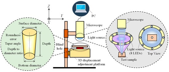
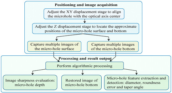
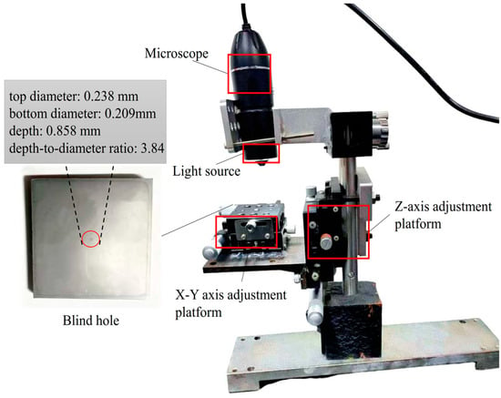
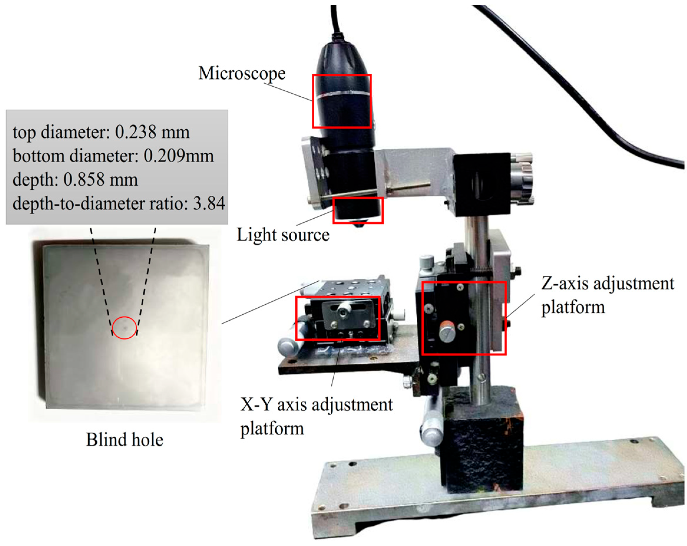
Figure 1 is a structural schematic of a high-aspect-ratio blind hole. The geometric metrics investigated in this work include microhole depth, top and bottom diameter, relative ellipticity deviation, taper angle, and depth-to-diameter ratio.
Figure 1.
Structure of the blind hole and measurement setup.
A machine-vision microscopic inspection platform was constructed for the comprehensive geometric measurement of high-aspect-ratio blind holes, as schematically illustrated in Figure 1. The primary components of the system are an annular illumination module, a digital microscope, a three-dimensional translation stage, and a host computer. At the Z-axis stage, the axial distance between the specimen and the microscope is adjusted, while the microhole center is aligned with the optical axis at the X/Y stages. The host computer acquires the microscopic images and performs subsequent image-processing and geometric-parameter calculations.
Illumination insufficiency at the bottoms of holes constitutes a major obstacle to high-aspect-ratio microhole measurement. To elevate the SNRs of bottom micrographs, a physical optical propagation model of microcavities was established based on Monte Carlo ray-tracing simulations. The results of the simulation indicate that omnidirectional light irradiation from an annular light source penetrates narrow, deep microholes more effectively and results in uniform light distribution across the bottom of the hole, drastically mitigating occlusion artifacts and imaging blind spots induced by unilateral lighting. Accordingly, the measurement platform features eight LED light sources uniformly distributed on a circular track with a radius of 4.0 mm that is concentric with respect to the main optical axis of the imaging system.
2.2. Measurement Workflow
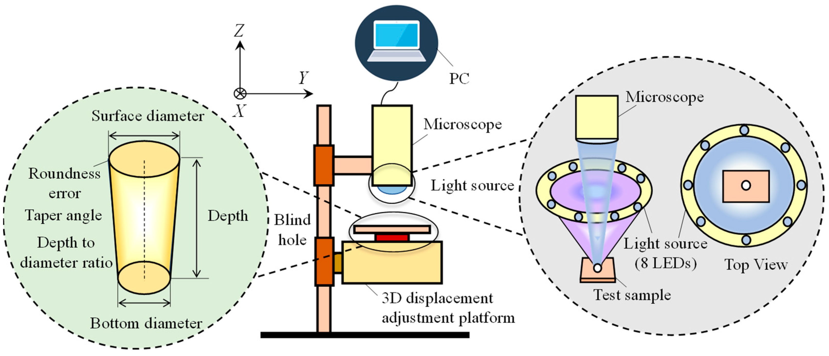
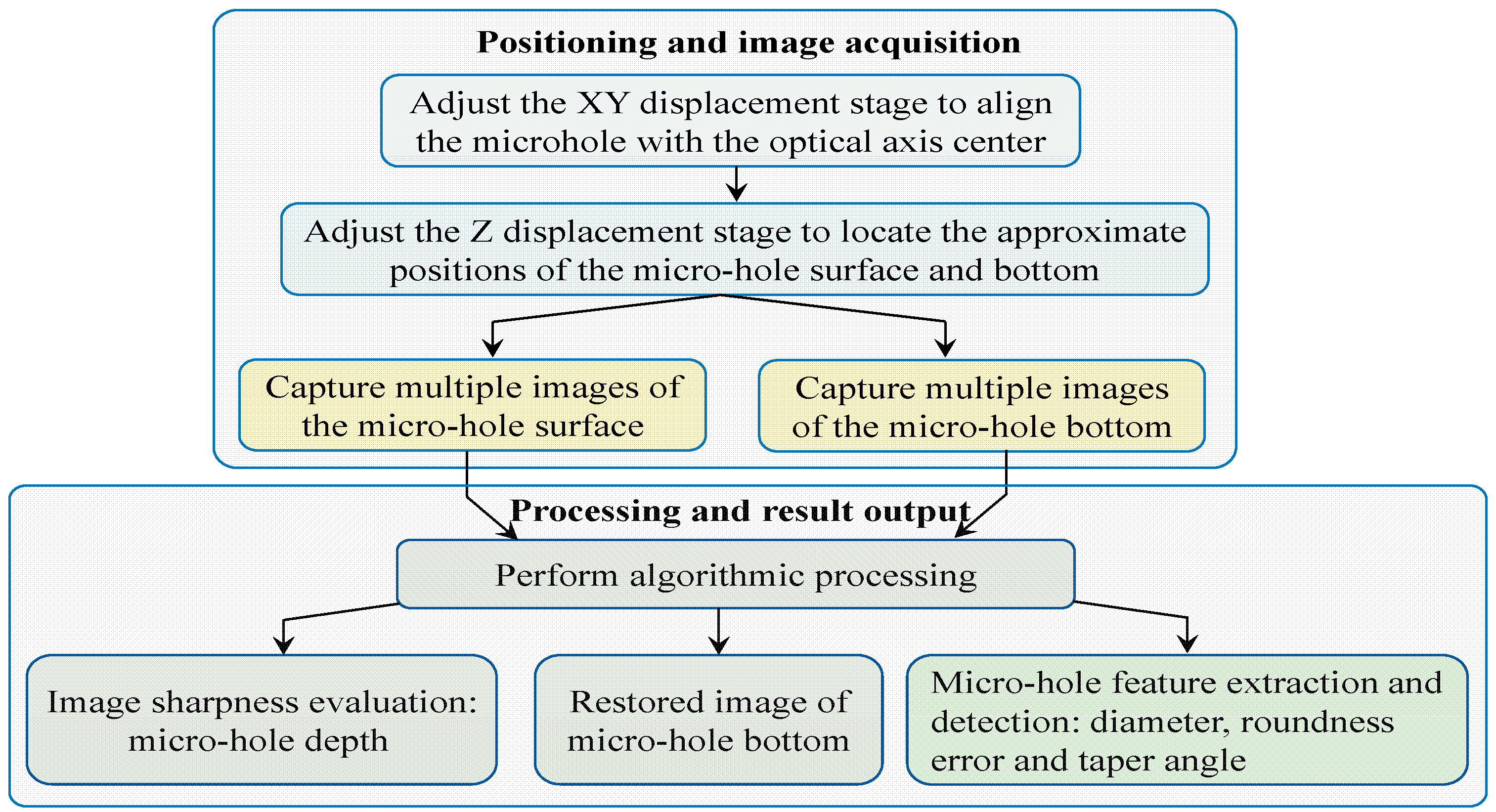
The complete measurement pipeline is summarized in Figure 2. First, the test specimen is fixed on the translation stage, and the X/Y axes are calibrated to center the target microhole within the imaging field of view. The Z-axis stage is then coarsely scanned to identify the axial range in which the microhole surface forms a clear focal plane, with the corresponding coordinate interval recorded. During coarse tuning for the microhole bottom, partial textures of the hole bottom and hole wall can be observed to sharpen. Such an observation can already constrain the coordinate range for clear imaging of the microhole bottom. The fine scan initiates approximately 60 μm below this position and moves upward at a step interval of 10 μm over a total travel of at least 120 μm, ensuring that the optimal surface focal position falls within the scanning range. The acquired image sequence is processed via Laplacian variance sharpness quantification coupled with local quadratic polynomial fitting to extract surface geometric parameters, including top diameter and top relative ellipticity deviation.
Figure 2.
Flowchart of the microhole measurement workflow.
The same scanning procedure is repeated for the bottom of the microhole to obtain the bottom geometric features. Given the inherently low SNR of bottom micrographs, a DnCNN-based image restoration module is employed prior to feature extraction to refine image quality and guarantee accurate dimensional calculation of the bottom of the hole. Microhole depth is derived from the calibrated axial coordinates: Z1 and Z2 denote the optimal focal positions of the microhole’s surface and bottom, respectively, and depth is calculated as the coordinate difference between Z1 and Z2. The measured depth and aperture values are further combined to compute the microhole’s depth-to-diameter ratio.
The overall microhole parameter calculation framework comprises three main modules, the first of which is an image sharpness evaluation algorithm. Laplacian variance is used to quantify image sharpness, which is further combined with local quadratic polynomial fitting to pinpoint the optimal Z-axis focal position of the micrographs. The second module is a hole-bottom image restoration algorithm. A DnCNN-based restoration algorithm is designed to reconstruct high-quality bottom micrographs from noisy, blurred inputs, enabling precise dimensional measurement of the hole bottom geometry. The third module is a microhole feature measurement algorithm. This pipeline integrates image preprocessing, adaptive threshold segmentation based on Otsu’s maximum between-class variance method, morphological denoising, and geometric parameter calculation through ellipse fitting.
3. Microhole Image-Processing Algorithms
3.1. Image Sharpness Evaluation Algorithm
During visual inspection of high-aspect-ratio microholes, accurate extraction of Z-axis coordinates corresponding to the optimal focal planes of the surfaces and bottoms of microholes is essential for reliable depth measurement. Manual visual sharpness assessment introduces subjective errors, stemming from the limited depth of field of optical systems and individual differences in human visual sensitivity. To eliminate subjective bias, Laplacian variance was selected as the quantitative sharpness evaluation metric for both raw surface micrographs and DnCNN-reconstructed bottom micrographs.
For a discrete 2D digital image I(x, y), the Laplacian convolution response L(x, y) is defined as follows:
where H represents the Laplacian convolution kernel. The Laplacian variance (LV) across the full image domain serves as the sharpness scoring index, expressed as follows:
where M and N correspond to image height and width, and denotes the average Laplacian response over the entire image. A larger LV value indicates a higher focusing degree and clearer image texture.
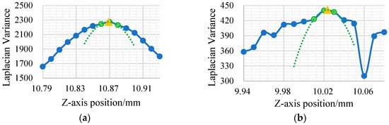
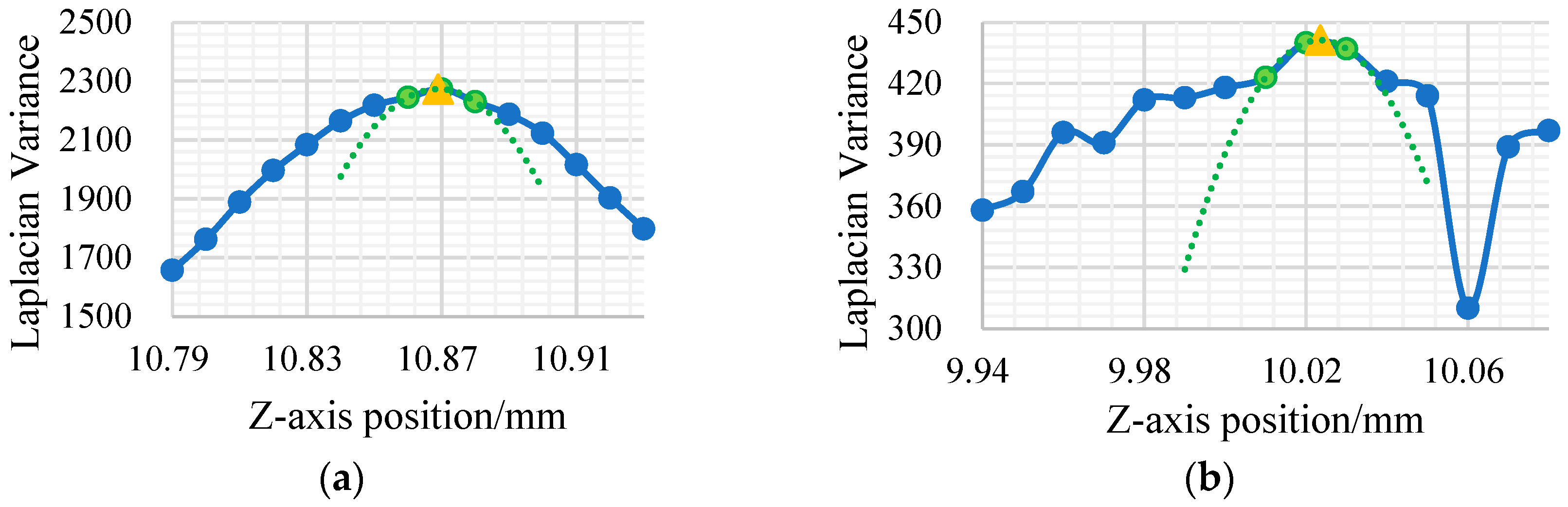
As a quantitative focus metric, Laplacian variance reaches its global maximum when the optical system achieves perfect focus. During measurement, one micrograph is captured every 10 μm along the Z-axis, and the Laplacian variance in each frame is computed to generate discrete sharpness curves for the surfaces and bottom of a microhole, as plotted in Figure 3.
Figure 3.
Laplacian variance curves of captured micrographs. (a) Microhole surface. (b) Microhole bottom.
Since discrete sampling points rarely align exactly with the true peak of the Laplacian variance curve, local quadratic polynomial fitting is introduced to improve depth measurement precision. Specifically, the sampling point with the maximum LV value and its two adjacent neighboring points are used for quadratic curve fitting. The vertex coordinate of the fitted parabola is designated as the precise Z-axis focal position. Because the fitted vertex provides a continuous Z-axis coordinate, the focal position can be estimated between two adjacent sampling positions rather than being restricted to discrete 10 μm intervals. This refinement represents a sub-sampling interpolation of the focus-curve maximum and does not imply an improvement in the physical resolution or positioning accuracy of the Z-stage. This strategy achieves high sub-sampling positioning accuracy for both the surface and bottom planes of microholes while maintaining low computational overhead.
3.2. DnCNN-Based Hole-Bottom Image Restoration Algorithm
DnCNN, developed by Zhang et al. [11], is a representative deep-learning image-denoising architecture based on residual learning. Its network backbone consists of stacked 3 × 3 convolution layers, batch normalization (BN), and Rectified Linear Unit (ReLU) activation functions. In this study, DnCNN is employed to suppress image noise and enhance the visibility of hole-bottom boundaries, thereby providing clearer contours and more reliable dimensional information for subsequent geometric measurement. It is not designed to recover precise pixel-level morphological information of the inner hole-bottom surface.
Supervised deep learning image restoration models typically require massive paired cleaned–degraded image datasets for training. However, collecting authentic paired ground-truth data poses significant practical challenges for high-aspect-ratio microhole measurements. When an objective lens focuses on the bottom of a microhole, narrow deep cavity walls create physical occlusion, and multiple internal light reflections interfere with photon transmission, drastically reducing the photon flux received by the imaging sensor. Consequently, it is infeasible to capture noise-free, uniformly illuminated micrographs of the bottoms of holes, severely restricting the training convergence of conventional end-to-end supervised networks.
To address the scarcity of authentic paired training data, we propose a synthetic degradation strategy that generates simulated low-quality bottom micrographs by artificially degrading clear surface micrographs. High-fidelity texture micrographs of flat sample surfaces are acquired and then subjected to multi-physics degradation operations to synthesize noisy, blurred samples that mimic real measurement conditions.
The mathematical degradation model is constructed via the following core steps. Under annular ring illumination, high-magnification micrographs of the flat-top surface of the sample were captured to obtain a set of clean ground-truth images Igt(x, y) that retain distinct machining textures and microscale material features.
During Z-axis focal scanning targeting the bottoms of holes, the microscope exhibits an ultra-shallow depth of field, while the illumination intensity decays radially from the center to the periphery of the bottom of the hole. Accordingly, a Gaussian blur kernel is adopted to simulate optical defocusing effects, and a radial vignetting function is introduced to model physical light attenuation:
where G(x, y, σblur) denotes a Gaussian blur kernel with a randomly sampled standard deviation within a predefined range, and A(x,y) is a spatially varying brightness attenuation matrix, defined as
where α is the global brightness-retention coefficient used to simulate the reduced luminous flux at the microhole bottom, and β is the radial vignetting coefficient. In the dataset-generation procedure, α and β were randomly sampled from [0.3,0.5] and [0.3, 0.6], respectively. D(x,y) is the dimensionless radial distance calculated after independently normalizing the horizontal and vertical pixel coordinates of the region of interest to [−1, 1]. Therefore, D(x,y) ranges from 0 at the image center to a maximum of two at the corners. The min(D(x,y),1) operation limits the radial term to [0,1]. Consequently, A(x,y) remains within [α(1 − β), α], corresponding to a physically meaningful positive brightness-retention factor without intensity amplification:
where NGaussian represents zero-mean signal-independent Gaussian noise used to simulate camera thermal and electronic noise, and NPoisson(x,y) represents the zero-mean signal-dependent Poisson perturbation used to simulate photon shot noise. The mixing coefficient λ controls the relative contributions of the two noise components and is randomly sampled from [0,1] for each degraded image; consequently, the Gaussian and Poisson weights are λ and 1 − λ, respectively. The Gaussian standard deviation σ is randomly selected from [2, 8] gray levels to generate different levels of signal-independent noise. For the Poisson component, the image intensity is first normalized to [0, 1], multiplied by a scaling parameter s = 256, and then used as the intensity parameter of the Poisson distribution. The sampled Poisson image is rescaled to [0, 255], and the original image intensity is subtracted to obtain a zero-mean Poisson perturbation. The parameter ranges were empirically selected to cover the noise variations observed in the acquired low-light microhole-bottom images. Finally, the degraded image is clipped to the valid 8-bit grayscale range of [0, 255].
The degradation parameters were empirically selected by referring to the visual characteristics and intensity variations observed in the acquired microhole-bottom images. Specifically, Gaussian kernels of 3 × 3, 5 × 5, 7 × 7, and 9 × 9, with standard deviations ranging from 0.5 to 2.0, were used to represent different degrees of optical blur. The global brightness-retention coefficient α and radial-vignetting coefficient β were randomly sampled from [0.3, 0.5] and [0.3, 0.6], respectively, to cover the overall intensity reduction and center-to-edge attenuation observed at the microhole bottom. The standard deviation of the Gaussian noise was randomly selected from two to eight gray levels, while the relative Gaussian–Poisson noise weight was randomly sampled from [0, 1]. Rather than reproducing one fixed degradation condition, random parameter sampling was adopted to cover a range of blur, brightness, contrast, and noise variations and thereby reduce the sensitivity of the DnCNN to a specific degradation setting.
Based on the proposed degradation algorithm, image pairs with variable blur strength, illumination attenuation, and SNR levels are randomly generated within the target microhole diameter range, as demonstrated in Figure 4. After data screening, a deep learning dataset containing 2000 image pairs is constructed, with 90% allocated for network training and 10% for validation, providing sufficient data support for DnCNN parameter optimization.
Figure 4.
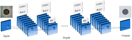
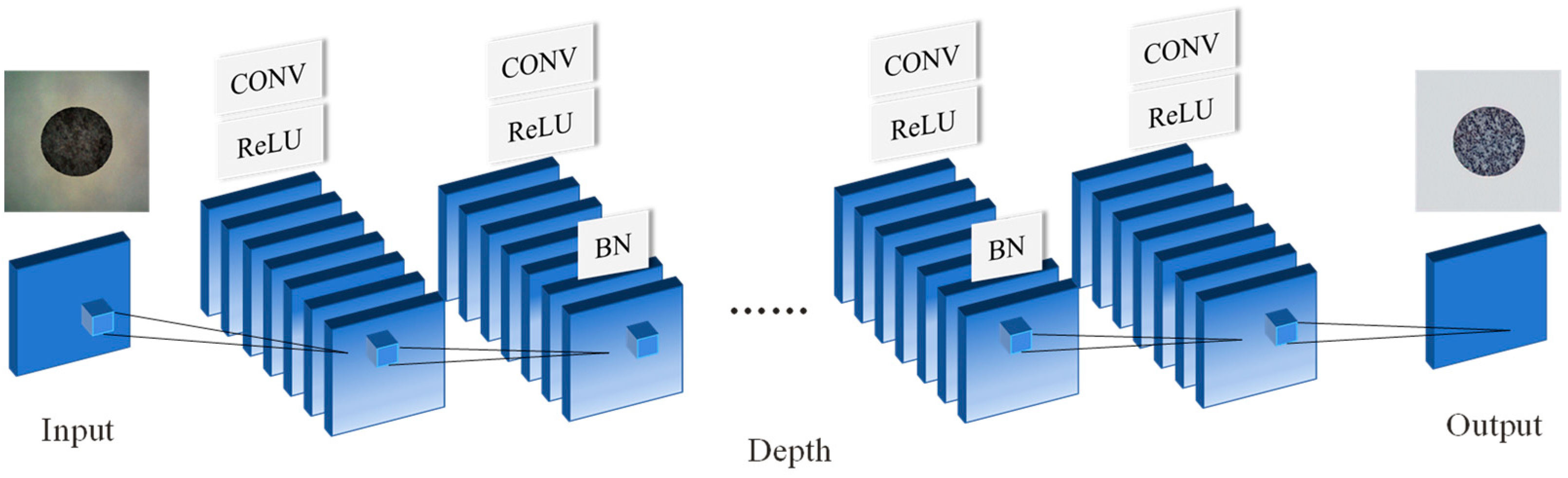
Schematic architecture of the DnCNN restoration network.
After DnCNN network initialization, the hyperparameters are configured as follows: The Adam optimizer is adopted for gradient descent optimization, with an initial learning rate of 0.001 and a cosine annealing schedule to gradually decay the learning rate to a minimum value of 0.000001. The L2 regularization weight decay factor is set to 0.00001, the mini-batch size is fixed at four, and the maximum training epoch is limited to 30. The synthesized 2000 pairs of degraded input images and corresponding clean images are utilized for network training.
The DnCNN adopted in this study contains 20 convolutional layers in total and does not include pooling layers. As illustrated in Figure 4, the first layer consists of a 3 × 3 convolutional layer followed by a rectified linear unit (ReLU) activation function. The subsequent 18 hidden layers each consist of a 3 × 3 convolutional layer, batch normalization (BN), and ReLU activation. The final output layer contains only a 3 × 3 convolutional layer, without BN or ReLU, and is used to predict the residual image.
For 20 consecutive 3 × 3 convolutional layers with a stride of one, the receptive field of the network is 41 × 41 pixels. The network was trained using residual learning, and the degraded image was used as the input, while the difference between the degraded and clean images was used as the learning target. The predicted residual was subsequently used to obtain the restored image. Batch normalization was applied in the hidden layers before nonlinear activation to stabilize the feature distribution and accelerate network convergence.
3.3. Microhole Feature Measurement Algorithm
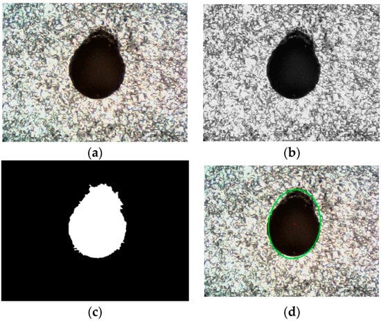
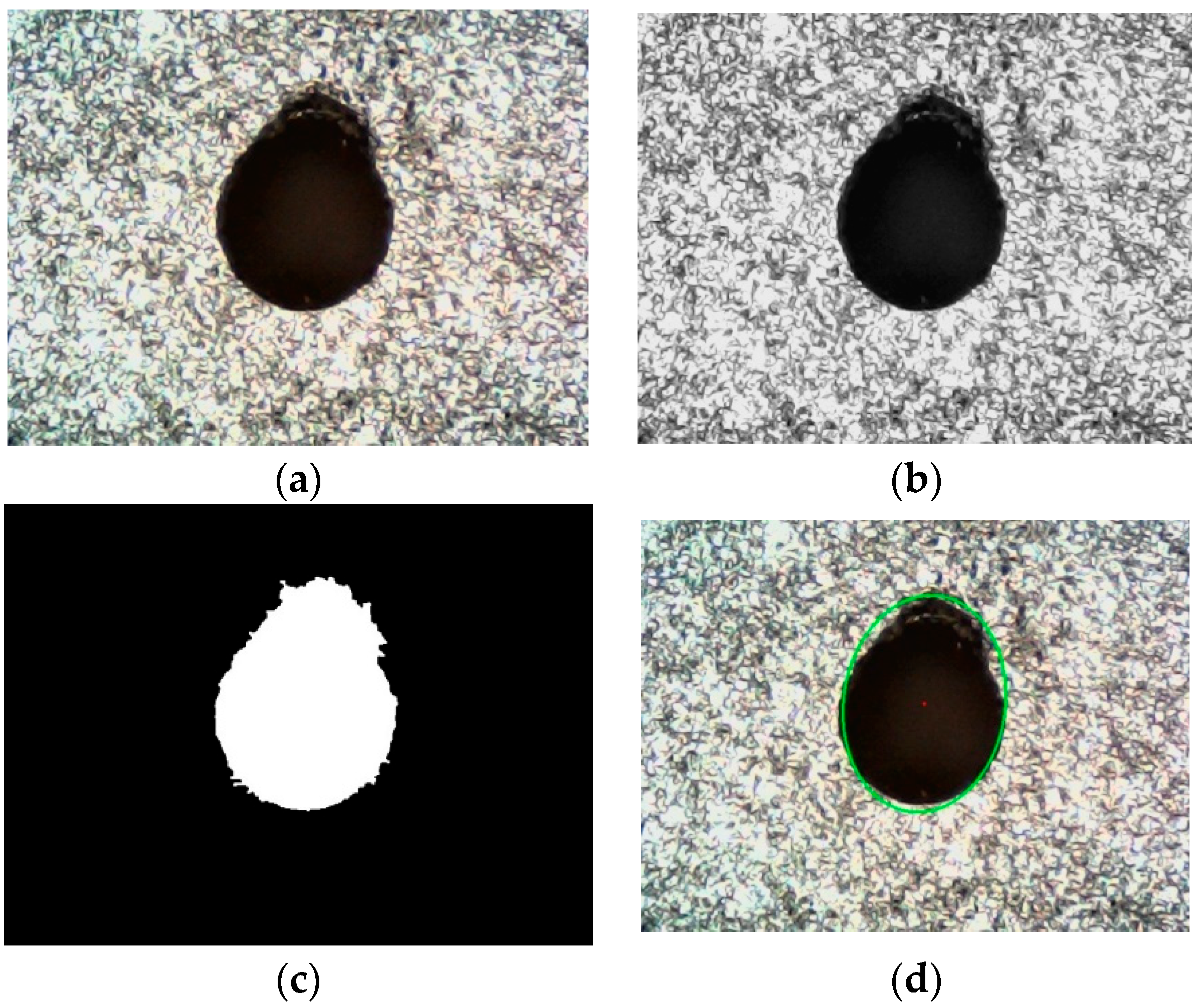
A machine vision automatic feature extraction algorithm was developed to quantify microhole surface geometric attributes. It consists of four sequential steps: image preprocessing, adaptive threshold segmentation, morphological noise suppression, and ellipse-fitting-based parameter calculation. The raw microhole micrograph prior to processing is presented in Figure 5a.
Figure 5.
Processing flowchart of the microhole feature measurement algorithm. (a) Raw microhole micrograph. (b) Grayscale image. (c) Binary image. (d) Ellipse-fitted image.
First, the captured RGB micrograph is converted into a single-channel grayscale image to reduce computational load and eliminate redundant color channel information, as shown in Figure 5b. Meanwhile, a 5 × 5 Gaussian convolution kernel is applied for spatial smoothing, achieving a balanced trade-off between high-frequency noise suppression and preservation of the fine details of the edges of microholes.
Otsu’s maximum inter-class variance method is then implemented for adaptive global threshold segmentation. By traversing all feasible grayscale levels, the algorithm automatically identifies the optimal binarization threshold in terms of maximizing the grayscale variance between target microhole regions and the background. Combined with inverse binarization, microhole pixels are assigned a value of 255 (white), and background pixels are set to 0 (black), generating the binary mask shown in Figure 5c.
To remove isolated pixels and small edge artifacts from the binary image, a morphological opening operation is employed. Specifically, a 3 × 3 all-one structural element executes erosion to remove fine protrusions and discrete noise spots, followed by dilation to restore the complete contour of the target microhole.
After a high-quality binary mask is acquired, a newly designed contour-filtering algorithm is employed to eliminate residual background artifacts in real captured images, as shown in Table 1.
Table 1.
Contour-filtering algorithm.
Contour validation is conducted before target selection to enhance measurement robustness and satisfy the minimum point requirement for ellipse fitting. Microholes fabricated via precision machining are rarely perfectly circular; hence, least-squares ellipse fitting is employed to approximate the microhole boundary, as visualized in Figure 5d. Fitting the extracted contour points yields a parametric geometric model, from which the microhole center coordinates (X, Y), major axis diameter Dlong, and minor axis diameter Dshort are extracted. The equivalent microhole diameter D is defined as the diameter of a circle having the same area as the fitted ellipse and is calculated as
This area-equivalent definition was selected because the microhole boundary is generally not perfectly circular. It considers the dimensions along both principal axes and converts the fitted elliptical boundary into a single representative diameter while preserving its cross-sectional area, thereby facilitating subsequent calculation and comparison of the microhole geometric parameters.
The taper angle of the microhole was calculated from the top diameter, bottom diameter, and hole depth as follows:
where Dtop and Dbottom are the equivalent diameters of the top and bottom boundaries, respectively, and h is the measured hole depth. Here, θ represents the one-sided taper angle between the microhole wall and the hole axis.
After all algorithmic modules were integrated, detection experiments were carried out on individual microhole micrographs. The quantitative output results verify that the proposed pipeline rapidly locates microhole targets and computes equivalent diameters automatically. The dimensional difference between major and minor axes was further utilized to calculate microhole relative ellipticity deviation.
4. DnCNN Model Evaluation and Measurement Experiments
4.1. Experimental Setup and Reference Measurement
The experimental setup is shown in Figure 6. A digital microscope incorporating a 2-megapixel camera was used to acquire images at a resolution of 1920 × 1080 pixels. The digital microscope delivers a 20× magnification factor with a native depth of field of 60 μm. A three-dimensional translation stage with a nominal positioning resolution of 10 μm along the X, Y, and Z axes was used for specimen positioning. During focal scanning, images were acquired at nominal Z-axis intervals of 10 μm.
Figure 6.
Photograph of the experimental measurement system.
The illumination module consisted of eight LEDs uniformly arranged on an annular support, with an angular interval of approximately 45° between adjacent LEDs. The annular light source had a radius of approximately 4 mm and was positioned 23 mm above the specimen surface. Its center was aligned with the microscope optical axis and the microhole center. Based on this geometry, the nominal illumination angle relative to the specimen normal was approximately 9.9°. Thus, this near-axial annular illumination enhanced light delivery into the blind hole and reduced directional shadows during image acquisition.
A standard calibrated microhole was used as the test specimen. The reference values of the microhole were as follows: top diameter, 0.238 mm; bottom diameter, 0.209 mm; depth, 0.858 mm; and depth-to-diameter ratio, 3.84. These dimensions were measured using a laser scanning confocal microscope (VK-X1000, KEYENCE, Osaka, Japan), with the height and width measurement resolution being 0.5 nm and 1 nm, respectively.
4.2. Quantitative Evaluation of DnCNN Restoration Performance
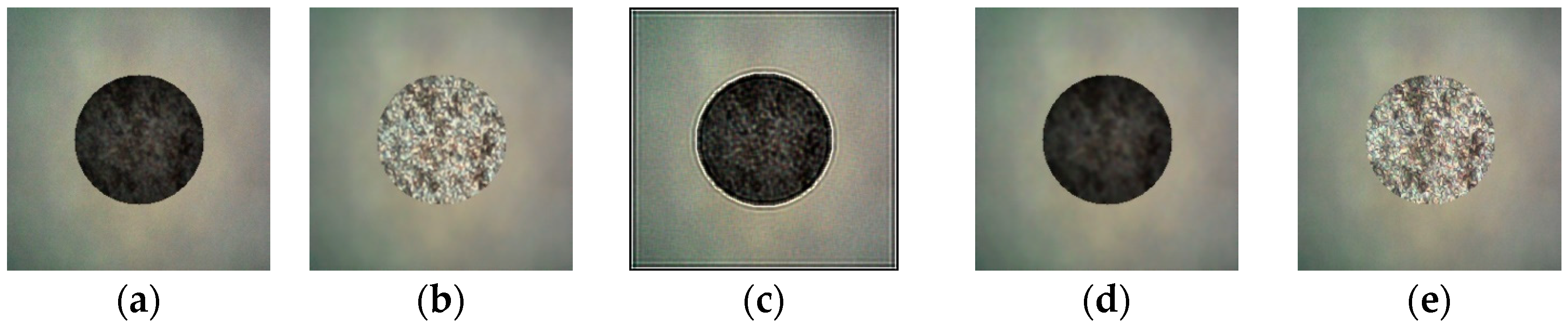
To validate the image restoration capacity of the proposed DnCNN network, its output results are compared with those achieved using conventional filtering techniques, including the Lucy–Richardson deconvolution algorithm and Wiener filtering, on identical degraded micrographs. The Peak Signal-to-Noise Ratio (PSNR) was adopted as the quantitative image quality metric, with comparative results illustrated in Figure 7 and summarized in Table 2.
Figure 7.
Comparison of restoration performance between traditional filtering algorithms and the proposed DnCNN network. (a) Original bottom image. (b) DnCNN. (c) Lucy–Richardson algorithm. (d) Wiener filtering. (e) Clear surface image.
Table 2.
PSNR quantitative comparison of different image restoration methods.
Figure 7a shows the original simulated low-SNR hole-bottom image. Figure 7b–d present restored images of Figure 7a using DnCNN, the Lucy–Richardson algorithm and Wiener filtering, respectively. Figure 7e shows a clear surface image, representing ideal restoration performance. The results indicate that image quality significantly improved after processing with the DnCNN model, and the restored images more closely resemble the actual hole-bottom morphology. The PSNR reached 28.25 dB, which was higher than the values obtained using the other methods, indicating that the reconstructed images are clearer and less noisy. These results indicate that the proposed model provides better restoration performance than the traditional algorithms and has the potential to improve the accuracy of subsequent microhole measurements. The reported PSNR values are the mean results calculated over the 200-image validation set.
To quantitatively evaluate the contribution of DnCNN restoration to the measurement results, the same measurement procedure was applied to the real microhole-bottom images before and after restoration. Before DnCNN restoration, the measured bottom diameter and depth were 0.194 mm and 0.842 mm, corresponding to absolute deviations of 15 μm and 16 μm from their reference values respectively. After DnCNN restoration, the measured bottom diameter and depth were 0.202 mm and 0.850 mm, and the corresponding absolute deviations decreased to 7 μm and 8 μm, respectively. This comparison indicates that DnCNN restoration improves the agreement of both diameter and depth measurements with their reference values.
4.3. Measurement Results
Repeated measurement tests were performed on the specimen, as shown in Figure 6. All measurement results are summarized in Table 3. Specifically, the depth-to-diameter ratio is the ratio of microhole depth to the average equivalent diameter measured at the top and bottom surfaces. The relative ellipticity deviation is expressed as the ratio of the major–minor axis difference in the fitted ellipse to the average diameter. The taper angle is derived from the diameter difference between top and bottom surfaces and the hole depth based on geometric relations.
Table 3.
Measurement results for a micro-blind hole.
The five repeated measurement trials exhibit favorable repeatability. The standard deviations of the top diameter, bottom diameter, depth, the depth-to-diameter ratio, relative ellipticity deviation, and taper angle are 0.002 mm, 0.003 mm, 0.003 mm, 0.04, 0.001, and 0.100°, respectively. Specifically, the depth-to-diameter ratio is the ratio of microhole depth to the average equivalent diameter of the top and bottom surfaces. The taper angle is derived from the top–bottom diameter difference and hole depth via geometric relations. The relative ellipticity deviation is expressed as the ratio of the major–minor axis difference in the fitted ellipse to the average diameter. The relative ellipticity deviation of the top and bottom surfaces was calculated separately, and their arithmetic mean was reported as the overall relative ellipticity deviation of the microhole.
For depth measurement, the average measured depth reached 0.850 mm, with an absolute deviation of 0.008 mm against the standard value. This result confirms that the combination of Laplacian variance sharpness scoring and three-point quadratic polynomial peak fitting effectively overcomes measurement limitations induced by limited optical depth of field and stage-positioning resolution, enabling micrometer-level depth quantification.
In terms of diameter measurement, the average top diameter reading was 0.234 mm, corresponding to an absolute deviation of 4 μm. Bottom diameter measurement presents greater technical challenges: high depth-to-diameter ratios trigger severe optical signal attenuation and scattering at the bottoms of microholes, decreasing accuracy for conventional microscopic inspection. Benefiting from the high-fidelity reconstruction capacity of the DnCNN network, the proposed method recovers complete texture and edge information from blurred, noisy bottom micrographs. The average measured bottom diameter was 0.202 mm, with absolute deviation controlled within 7 μm.
Additional geometric indicators, including the depth-to-diameter ratio, taper angle, and ellipticity deviation, were calculated. The mean measured depth-to-diameter ratio was 3.90, deviating from the reference value of 3.84 by 0.06. As shown in Table 3, the mean taper angle was 1.077°, with a sample standard deviation of 0.100°. Compared with a reference taper angle of 0.968°, the mean deviation was 0.109°. This relatively large angular deviation is mainly attributed to the propagation of the top- and bottom-diameter deviations. The mean ellipticity deviation was 0.032, with a sample standard deviation of 0.001. Its minor variation across repeated measurements may be attributed to machining-induced boundary irregularities and partial light occlusion by the microhole walls. Overall, the results demonstrate that the proposed method provides stable and comprehensive geometric characterization of the tested high-aspect-ratio micro-blind hole.
4.4. Discussion
For blind-microhole measurement, diameter and depth are the two fundamental geometric quantities, from which other parameters, such as the depth-to-diameter ratio and taper angle, are derived. Their measurement uncertainties may arise from multiple coupled factors, including optical-system calibration, stage positioning, image quality and focal-position localization. Because some hardware- and environment-related contributions are difficult to isolate and quantify independently under the present experimental conditions, and the present study focuses on the proposed image-processing and measurement algorithms, this section primarily evaluates the uncertainty-related contributions associated with image-preprocessing parameter selection and quadratic peak localization. The random measurement error is characterized by measurement repeatability.
For diameter measurement, the main uncertainty sources are boundary localization, ellipse fitting, and preprocessing-parameter selection. The ellipse-fitting quality was evaluated using the RMSE of the distances between the extracted contour points and the fitted ellipse. The mean RMSEs were 1.18 μm for the top boundary and 1.72 μm for the bottom boundary, corresponding to only 0.50% and 0.85% of their measured equivalent diameters, respectively. These relatively small ratios indicate that the fitted ellipses provide a reasonable representation of the extracted boundaries. The larger RMSE at the hole bottom is attributed to its lower SNR and less stable boundary localization. The sensitivity of diameter extraction to preprocessing parameters was further evaluated. Using the 5 × 5 Gaussian kernel, 3 × 3 morphological structuring element, and Otsu threshold as the baseline settings, the Gaussian kernel varied among 3 × 3, 5 × 5, and 7 × 7; the morphological structuring element varied between 3 × 3 and 5 × 5; and the Otsu threshold varied by ±5 gray levels. Within these ranges, the maximum absolute variations in the fitted major-axis diameter, minor-axis diameter, and equivalent diameter were 2.3 μm, 2.6 μm, and 2.1 μm, respectively, while the maximum change in ellipticity deviation was 0.005. Threshold variation produced the largest change, particularly for the low-SNR bottom boundary, whereas variations in the Gaussian and morphological kernel sizes had smaller effects. After combining the algorithm-related and random uncertainty components, the expanded uncertainties of the top and bottom diameters were estimated as 2.90 μm and 3.66 μm, respectively. The larger uncertainty of the bottom diameter is consistent with its higher fitting RMSE and greater sensitivity to threshold variation. Overall, the results indicate that the selected preprocessing and ellipse-fitting procedure provides acceptable robustness, although bottom-boundary localization remains the dominant uncertainty source in diameter measurement.
For depth measurement, the uncertainty associated with sub-sampling focal-position estimation was evaluated from the measured Laplacian-variance curves. Let f(z) denote the Laplacian variance at the Z-axis position z, and let z denote the sampled position corresponding to the maximum Laplacian variance. The five sharpness values used for the error analysis are expressed as yk = f(z0 + kh), where k = −2,−1,0,1,2 and h = 10 μm is the axial sampling interval. It should be noted that these five points were used only to estimate the local derivatives for uncertainty analysis, whereas the actual quadratic focal-position fitting was performed using the maximum point and its two immediately adjacent points.
The following analysis is based on a Taylor expansion of the sharpness curve near its maximum. The derivatives were estimated using standard five-point central-difference formulas, and the localization error was obtained from the leading-order truncation error of the local quadratic approximation. Assuming that the sharpness curve is locally smooth near its maximum, the second- and third-order derivatives at z were estimated using the five-point central-difference formulas:
The leading-order localization error associated with the local quadratic approximation was then estimated as follows:
where Eloc has the same unit as the Z-axis coordinate and represents the estimated deviation caused by the local asymmetry of the sharpness curve. A larger value of f‴(z0)/f″(z0) indicates stronger local asymmetry relative to the peak curvature and consequently a greater potential localization error. Substitution of the measured sharpness values into Equations (8)–(10) yielded localization-error estimates of approximately 1.38 μm and 1.55 μm for the top and bottom focal positions, respectively. Assuming that these two components are independent, their root-sum-of-squares combination gives a quadratic-fitting-related depth uncertainty of approximately 2.08 μm. Further incorporating the random error, the total depth uncertainty amounts to 3.65 μm.
The standard uncertainties of the derived depth-to-diameter ratio and taper angle were then evaluated using first-order uncertainty propagation. Substitution of the measured mean values and repeatability components yielded the standard uncertainty of the depth-to-diameter ratio of 0.035 and the standard uncertainty of the taper angle of 0.12°. These estimates are consistent with the observed repeatability of 0.04 and 0.100°, respectively, and confirm that the taper angle is more sensitive to the combined top- and bottom-diameter uncertainties because it depends on their relatively small difference. Specifically, the measured difference between the mean top and bottom diameters was 0.032 mm, whereas the corresponding reference diameter difference was 0.029 mm. Although the difference between these two values is only 3 μm, it represents a relative change of approximately 10.3% in the small diameter difference used to calculate the taper angle. Moreover, the measured depth of 0.850 mm was slightly smaller than the reference value of 0.858 mm, which further increased the calculated taper angle. Therefore, the taper angle is more sensitive to diameter and depth deviations than the individual dimensional measurements.
Overall, the results show that diameter measurement is mainly affected by bottom-contour localization and image restoration, whereas depth measurement is jointly affected by Z-axis repositioning, image quality, and quadratic-fit peak localization. The reported values therefore characterize the algorithm-related contributions and systematic random-error contributions of the proposed measurement system rather than its complete measurement uncertainty.
5. Conclusions
To address the challenge of high-precision geometric measurement of high-aspect-ratio blind holes, we propose a deep-learning-driven image reconstruction method for comprehensive geometric measurement. First, Laplacian variance-based sharpness evaluation combined with local quadratic polynomial fitting was applied to microscopic images to accurately locate the focal position along the vertical axis. This enabled high-precision measurement of the depth of microholes while eliminating reliance on subjective visual judgment. Second, to overcome the low signal-to-noise ratio of hole-bottom images, simulated degraded images were generated by inversely degrading sharp surface images, and the resulting paired dataset was used to train a DnCNN model for the high-fidelity reconstruction of hole-bottom images. Finally, a feature extraction algorithm integrating image preprocessing, adaptive threshold segmentation, and ellipse fitting was developed to achieve micrometer-level measurement of all geometric parameters of microholes. The experimental results showed that absolute deviations of the mean measured r surface diameter, bottom diameter, and depth from their corresponding reference values were 4 μm, 7 μm, and 8 μm, respectively. Based on these measurements, the depth-to-diameter ratio, taper, and roundness error were calculated, with the depth-to-diameter ratio differing from the standard value by 0.06. These results validate the effectiveness and reliability of the proposed method, demonstrating its potential as a high-precision, low-cost, and non-destructive solution for comprehensive geometric measurement of high-aspect-ratio blind holes. Nevertheless, the current method has two main limitations. First, the device requires manual positioning and focal scanning of the top and bottom regions, which limits measurement efficiency. Second, the experimental validation was conducted using only one standard blind microhole. In future work, the automated linear guide motion mechanism will be optimized to develop a fully automated measurement system, thereby further improving measurement efficiency and accuracy. Meanwhile, more blind-hole specimens will be measured to further evaluate the applicability and robustness of the proposed method.
Author Contributions
Conceptualization, methodology, F.Z. and H.G.; software, X.C. and P.C.; validation, formal analysis, investigation, data curation, H.G., X.C., P.C., J.X. and D.W.; resources, Q.F. and F.Z.; writing—original draft preparation, H.G., X.C. and P.C.; writing—review and editing, F.Z.; visualization, H.G., X.C. and P.C.; supervision, project administration, funding acquisition, F.Z. All authors have read and agreed to the published version of the manuscript.
Funding
This research was funded by National Natural Science Foundation of China (No. 52305564) and the Fundamental Research Funds for the Central Universities (No. 2023JBZX004).
Informed Consent Statement
This research does not involve humans.
Data Availability Statement
The original contributions presented in this study are included in the article. Further inquiries can be directed to the corresponding author.
Conflicts of Interest
The authors declare no conflicts of interest.
References
- Wu, C.X.; Ma, J.Q.; Gao, Z.S.; Guo, Z.Y.; Yuan, Q. Aberration-compensated near-infrared microscopic interferometric measurement of silicon through-holes. Opt. Precis. Eng. 2023, 31, 301–312. [Google Scholar]
- Zhang, Y. Application research on microaperture testing methods based on the Airy disk measurement method. Electr. Autom. 2010, 32, 80–81. [Google Scholar]
- Zhao, W.Q.; Tan, J.B.; Qiu, L.R. Bipolar absolute differential confocal approach to higher spatial resolution. Opt. Express 2004, 12, 5013–5021. [Google Scholar] [CrossRef] [Scilit] [PubMed]
- Wang, R.; Duan, F.J.; Fu, X.; Li, J. Method for measuring geometric dimensions of micro parts based on a telecentric camera. Opt. Express 2025, 33, 23580–23595. [Google Scholar] [CrossRef] [Scilit] [PubMed]
- Qian, B.; Guo, G.Q.; Qiu, L.; Wang, F.W.; Jin, L.; Fu, Y.J. Research on a method for measuring the parameters of high-precision circular holes based on subpixel edge detection. Aerospace 2017, 34, 126–132. [Google Scholar]
- Li, X.; Zhou, J.Y.; Xin, H.J.; Li, W.; Yin, X.; Yuan, X.A.; Ma, X. Vision measurement system for geometric parameters of tubing internal threads based on double-mirrored structured light. Opt. Express 2022, 30, 47701–47719. [Google Scholar] [CrossRef] [Scilit] [PubMed]
- Huo, X.; Wang, S.M.; Gao, Z.S.; Yuan, Q.; Li, Y.; Xu, Z.; Qiao, W. Dynamic compensation of modulation aberration in high-aspect-ratio composite trenches via a backpropagation neural network for topography measurement. Opt. Express 2025, 33, 48591–48606. [Google Scholar] [CrossRef] [Scilit] [PubMed]
- Lim, D.W.; Kim, M.; Choi, P. Hole depth prediction in a femtosecond laser drilling process using deep learning. Micromachines 2023, 14, 743. [Google Scholar] [CrossRef] [Scilit] [PubMed]
- Cao, Z.-H.; Tang, J.; Li, Z.; Chen, Y.-L. Full Cross-Sectional Profile Measurement of a High-Aspect-Ratio Micro-Groove Using a Deflection Probe Measuring System. Sensors 2025, 25, 2335. [Google Scholar] [CrossRef] [Scilit] [PubMed]
- Liu, Q.; Han, J.H.; Liu, M.; Xu, Y.R.; Liao, G.L. A study on microhole detection in fiber-optic probes based on an improved point Hough transform. Sens. Microsyst. 2020, 39, 9–12. [Google Scholar]
- Zhang, K.; Zuo, W.M.; Chen, Y.J. Beyond a Gaussian denoiser: Residual learning of deep CNN for image denoising. IEEE Trans. Image Process. 2017, 26, 3142–3155. [Google Scholar] [CrossRef] [Scilit] [PubMed]

Disclaimer/Publisher’s Note: The statements, opinions and data contained in all publications are solely those of the individual author(s) and contributor(s) and not of MDPI and/or the editor(s). MDPI and/or the editor(s) disclaim responsibility for any injury to people or property resulting from any ideas, methods, instructions or products referred to in the content. |
© 2026 by the authors. Licensee MDPI, Basel, Switzerland. This article is an open access article distributed under the terms and conditions of the Creative Commons Attribution (CC BY) license.