Performance Analysis of a Three-Hop Heterogeneous Space–Air–Sea Communication System with Adaptive Combining for Mixed FSO/RF and UWOC Transmission

Abstract

To meet the growing demand for reliable space–air–sea-integrated communications and underwater information backhaul, this paper proposes and analyzes a three-hop heterogeneous space–air–sea communication system consisting of a satellite, a high-altitude platform (HAP), a sea-surface buoy, and an autonomous underwater vehicle (AUV). Specifically, the satellite-to-HAP link employs free-space optical (FSO) transmission, the HAP-to-sea-surface buoy link adopts mixed FSO/radio-frequency (RF) transmission, and the sea-surface buoy-to-AUV link utilizes underwater wireless optical communication (UWOC). To enhance the reliability of the HAP-to-sea-surface buoy link in complex atmospheric and maritime environments, a threshold-based adaptive combining scheme for mixed FSO/RF transmission is designed. Meanwhile, nonzero-boresight pointing error models are incorporated into the FSO and UWOC links to characterize practical link misalignment. Based on the proposed system model, analytical expressions for the end-to-end bit error rate (BER) are derived and validated through Monte Carlo simulations. The numerical results show that the proposed adaptive combining scheme achieves better BER performance than conventional dual-hop and hard-switching schemes. In addition, the effects of pointing errors, underwater turbulence, underwater transmission distance, shadowed fading, detection techniques, and modulation schemes on the system BER performance are further investigated. This work provides theoretical guidance for reliable cross-domain heterogeneous transmission in future space–air–sea integrated communication systems.

1. Introduction

With the rapid development of sixth-generation (6G) mobile communications, the demand for wide-area coverage in remote maritime regions, sea-surface node access, and underwater information backhaul has been continuously increasing. Due to the lack of fixed communication infrastructure in open-ocean environments, it is difficult for conventional terrestrial networks to provide continuous and reliable communication services for sea-surface buoys, autonomous underwater vehicles (AUVs), and underwater sensor nodes. In contrast, satellites can provide wide-area coverage and long-distance information backhaul capabilities, while aerial platforms and sea-surface nodes can further enhance cross-domain access and relay transmission. Therefore, space–air–sea-integrated communications can provide effective support for remote maritime communications, the Internet of Underwater Things, and underwater data backhaul [1,2,3]. However, such systems span multiple propagation media, involve heterogeneous link architectures, and operate in complex channel environments. As a result, a single communication technology is difficult to simultaneously satisfy the requirements of a high data rate, low latency, and reliable transmission. Accordingly, it is of great significance to investigate the modeling and performance analysis of space–air–sea communication systems oriented toward multi-medium propagation and multi-link cooperative transmission.

In space–air–sea cross-domain communication scenarios, although satellites can provide wide-area coverage and long-distance information backhaul capabilities for remote maritime regions, direct satellite-to-sea surface transmission generally suffers from long propagation distances and is vulnerable to low-altitude atmospheric turbulence, cloud and rain attenuation, and pointing errors [4]. To improve link stability and regional access capability, a high-altitude platform (HAP) can be introduced as an important relay node between the satellite and sea-surface nodes [5]. Since the satellite-to-HAP link is usually required to support high-rate, low-latency, and large-capacity information transmission, free-space optical (FSO) communication is well suited for high-speed long-distance transmission between the satellite and the HAP due to its ultra-wide bandwidth, high data rate, immunity to electromagnetic interference, and license-free spectrum advantages [6].

The HAP-to-sea surface buoy link is a critical air–sea segment between the aerial platform and the sea-surface access node, and its transmission quality directly affects subsequent underwater information backhaul and the end-to-end system performance. Since the sea-surface buoy serves as a cross-media relay between the aerial link and the underwater link, investigating reliable transmission mechanisms for this link is beneficial for improving the access capability and transmission stability of space–air–sea cross-domain communication systems [7]. This link is required not only to support high-speed transmission but also to cope with complex environmental effects such as sea fog, rainfall, atmospheric disturbances, sea-surface reflection, and buoy attitude variations [8]. Although the FSO link can provide high-rate and large-capacity transmission, its performance is highly susceptible to atmospheric turbulence, weather conditions, and pointing errors. Therefore, a single FSO link can hardly maintain stable connectivity while guaranteeing high-speed transmission. In contrast, the radio-frequency (RF) link offers stable propagation, wide coverage, and strong environmental adaptability and can serve as a reliable complement when the FSO link is impaired.

For the sea-surface buoy-to-AUV link, the underwater environment is complex. Although conventional underwater acoustic communication (UAC) provides relatively long transmission ranges and strong environmental adaptability, it is constrained by narrow available bandwidth, low transmission rate, and large propagation delay, making it difficult to satisfy the requirements of high-speed, low-latency, and large-capacity underwater data transmission [9]. In contrast, underwater wireless optical communication (UWOC), with the advantages of a high data rate, low latency, a large bandwidth, and strong covertness, can effectively support short-range high-capacity transmission between sea-surface buoys and AUVs [10]. Based on these characteristics, the cooperative application of FSO, RF, and UWOC in a space–air–sea cross-domain heterogeneous transmission system provides a promising research direction for constructing efficient and reliable cross-domain communication networks.

At the network level, AUV mobility and deployment can affect UWOC link availability by changing the transmission distance, geometric alignment, and communication opportunities with underwater sensor nodes. Uncertainty-aware adaptive path planning can support AUV navigation in partially observed and time-varying underwater environments [11], while optimized multi-AUV placement can improve the coverage of seabed sensors by short-range optical communication links [12]. Although these network-layer optimization problems are beyond the scope of the present physical-layer BER analysis, they complement the current study and motivate future joint optimization of communication reliability, AUV trajectories, and multi-AUV sensor coverage.

With the increasing demands for the Internet of Underwater Things and underwater information backhaul, mixed communication systems from satellites to AUVs have gradually attracted research attention. Such systems usually adopt a dual-hop mixed transmission architecture consisting of a satellite, a sea-surface relay, and an AUV, where the satellite-to-sea-surface relay link employs RF transmission and the sea-surface relay-to-AUV link employs UWOC transmission, thereby enabling cross-media information transfer from satellite coverage to underwater access. For example, Gamal et al. constructed a non-orthogonal multiple access (NOMA)-based dual-hop mixed satellite–underwater communication system and analyzed the outage performance of different users, demonstrating the application potential of NOMA access in mixed satellite–underwater transmission [13]. Teng and He further investigated a dual-hop relay link for satellite–underwater communication by considering pointing errors and additive white generalized Gaussian noise, and analyzed the effects of link misalignment, air-bubble level, and underwater turbulence on system reliability [14]. Zhou et al. proposed a hybrid RF/UWOC dual-hop relay link for satellite–underwater communication and analyzed the influence of different link parameters on system reliability [15]. Overall, existing studies on mixed satellite–underwater communication systems remain relatively limited [13,14,15]. Therefore, further investigation into the modeling and performance analysis of mixed satellite–underwater communication systems is still necessary.

In related studies, existing works on cross-domain transmission from aerial platforms to AUVs can be mainly classified into two categories: direct cross-media transmission without sea-surface relays and relay-assisted segmented heterogeneous transmission. Although direct air-to-water transmission without relays has a simple structure and flexible deployment, the link is susceptible to air–water interface fluctuations, pointing errors, and propagation loss, making it difficult to maintain stable transmission under complex sea conditions [16]. In contrast, relay-assisted segmented transmission enables the aerial link and underwater link to be modeled separately, thereby reducing the difficulty of cross-media transmission and improving link reliability. For relay-assisted segmented transmission, a considerable number of studies have introduced unmanned aerial vehicles (UAVs) as aerial platforms into air-to-water cross-domain communication systems to improve cross-domain link quality and enhance transmission reliability. For example, Li et al. investigated a UAV-based mixed RF/UWOC system, focusing on the effects of UAV altitude, underwater air bubbles, temperature gradients, salinity variations, and detection techniques on the outage probability, average bit error rate, and average channel capacity [17]. Devaja et al. studied a UAV-based mixed RF/UWOC system and further analyzed the impact of sea-surface buoy relays and optimal relay selection on the outage performance [18].

However, in complex sea-surface environments, UAVs are vulnerable to sea-wind disturbances, platform vibration, and attitude variations, which may increase beam jitter and link alignment deviations, thereby degrading the transmission stability of air-to-water cross-domain links. By contrast, HAPs have quasi-stationary deployment characteristics and are typically located in the stratosphere at altitudes of 17–32 km. In this region, vertical atmospheric convection is relatively weak, the airflow environment is comparatively stable, and low-altitude atmospheric disturbances such as clouds, rainfall, and water vapor are less severe. Therefore, HAPs can, to some extent, reduce platform attitude disturbances and random link fluctuations, making them more favorable for maintaining stable optical link alignment. Meanwhile, HAPs also offer the advantages of wide coverage and strong continuous service capability. Nevertheless, studies employing HAPs as aerial platforms to support AUV communications remain rather limited. To the best of our knowledge, only Nallagonda et al. investigated a HAP-assisted dual-hop mixed RF/UWOC transmission system and verified the feasibility of this architecture in air-to-water cross-domain communication scenarios [19].

The closest prior systems fall into three groups. Satellite/HAP-to-underwater systems [14,19] use dual-hop RF/UWOC transmission and lack FSO/RF diversity in the air-to-sea hop. Although [20,21] also consider three-hop RF/FSO/UWOC transmission, neither establishes a satellite-originated space–air–sea route. Sarma et al. [20] connect a terrestrial source to an underwater destination through separate RF-FSO-UWOC hops, whereas Yadav et al. [21] connect a source, a UAV, a floating vehicle, and an underwater destination through separate FSO-RF-UWOC hops; neither architecture contains both a satellite source and a HAP relay. In contrast, the proposed satellite–HAP–buoy–AUV chain originates in the space segment and spans the space, air, sea-surface, and underwater domains. It also embeds threshold-triggered FSO/RF redundancy within the HAP-to-buoy hop rather than assigning FSO and RF to separate serial hops: the FSO branch operates alone when its instantaneous SNR is at or above the threshold; below it, the RF branch is activated, and the FSO/RF observations are combined by MRC. Hybrid FSO/RF has also been studied without an underwater segment [22] or in a two-phase terrestrial–underwater system [23], where multi-antenna MRC is applied within the RF branch. Nonzero-boresight pointing errors are further modeled in the satellite-to-HAP FSO link, the HAP-to-buoy FSO branch, and the buoy-to-AUV UWOC link. Table 1 summarizes these architectural and technical differences.

Table 1. Comparison of domain coverage and FSO/RF allocation in the closest related mixed relay systems and the proposed system.

Study	Architecture/Domain Coverage	Links	FSO/RF Treatment	Metrics
Teng and He [14]	Satellite–buoy–underwater; dual hop	RF/UWOC	No FSO/RF diversity; boresight error and AWGGN	OP, BER, and asymptotic
Nallagonda et al. [19]	HAP–buoy–underwater; dual hop	RF/UWOC	No FSO/RF diversity; DF relaying	Error rate
Bankey et al. [22]	Satellite–HAPS–ground	Hybrid FSO/RF	No underwater hop	SOP; asymptotic SOP
Sarma et al. [20]	Terrestrial source–relay–relay–underwater; no satellite/HAP	RF/FSO/UWOC	FSO and RF on separate hops	OP; BER
Yadav et al. [21]	Distant-island terrestrial source–UAV–floating vehicle–underwater; no satellite/HAP	FSO/RF/UWOC	FSO and RF on separate hops	OP; altitude optimization
Payal and Gurjar [23]	Base station–buoy–underwater; dual hop	Hybrid FSO/RF/UWOC	RF backup; MRC across RF antennas	OP, throughput, and capacity
This work	Satellite–HAP–buoy–AUV; satellite-originated space–air–sea route	FSO/adaptive FSO/RF/UWOC	Threshold RF activation; FSO/RF MRC; boresight errors in all optical links	BER and high-SNR asymptotic analysis

Recent studies have examined directly modulated optical wireless links. Alhalabi et al. analyzed a 16-QAM DCO-OFDM visible-light link under atmospheric turbulence, pointing errors, and adverse weather conditions [24], while Refs. [25,26] investigated low-cost DM-DD-OFDM optical links and evaluated their BER and related transmission performance without external optical modulators. Unlike these point-to-point optical-wireless systems, the present work analyzes the end-to-end BER of a satellite–HAP–buoy–AUV three-hop heterogeneous architecture integrating FSO, adaptive FSO/RF transmission, and UWOC under DF relaying.

Based on the above comparison, the main contributions are fourfold. First, we establish a DF-based end-to-end space–air–sea model comprising a satellite source, a HAP relay, a sea-surface buoy relay, and an AUV destination. Unlike existing terrestrial-to-underwater or UAV-assisted three-hop models [20,21], this architecture explicitly provides satellite-originated information backhaul across the space, air, sea-surface, and underwater domains. Its three serial hops are FSO, adaptive mixed FSO/RF, and UWOC, respectively, which places FSO/RF redundancy within the critical HAP-to-buoy hop rather than assigning FSO and RF to separate serial hops. Second, we develop a threshold-triggered combining rule: when the instantaneous FSO SNR is at or above the threshold, only the FSO branch is used; when it is below the threshold, the RF branch is activated, and the FSO and RF observations are combined by MRC. Third, practical nonzero-boresight pointing errors are incorporated consistently into the satellite-to-HAP FSO link, the HAP-to-buoy FSO branch, and the buoy-to-AUV UWOC link, together with the Málaga-$ℳ$, shadowed-Rician, and WGG fading models. Fourth, we derive and numerically validate an end-to-end BER framework for multiple modulation and detection configurations and identify the high-SNR diversity-order and coding-gain behavior of the complete heterogeneous route.

The remainder of this paper is organized as follows. Section 2 presents the system and channel models. Section 3 derives the end-to-end BER and high-SNR behavior. Section 4 provides numerical and Monte Carlo results, and Section 5 concludes this paper.

2. System Model

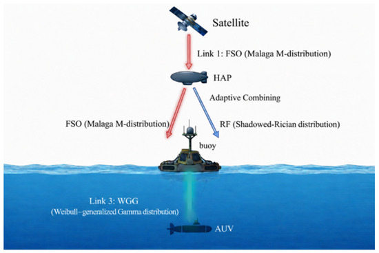
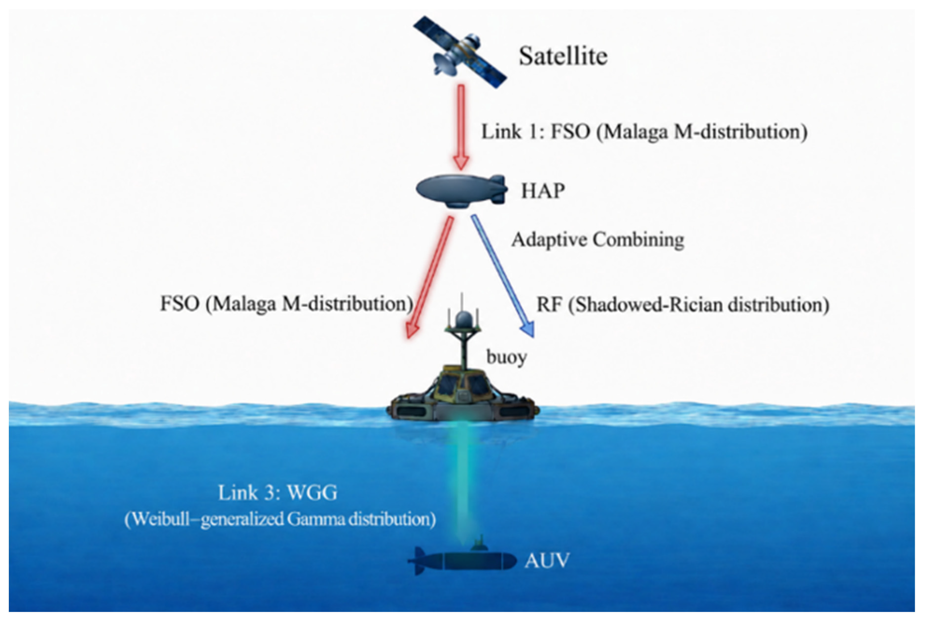
As shown in Figure 1, this paper considers a three-hop heterogeneous space–air–sea mixed communication system consisting of a satellite source node, a HAP relay, a sea-surface buoy, and an AUV, where both the HAP and the sea-surface buoy employ the decode-and-forward (DF) relaying protocol. Specifically, the first hop S→HAP is an FSO link, whose channel fading is modeled by the Málaga-$ℳ$ distribution with nonzero-boresight pointing errors. The second hop HAP→Buoy is a mixed FSO/RF link, where the FSO branch is characterized by the Málaga-$ℳ$ distribution with nonzero-boresight pointing errors, while the RF branch follows the shadowed-Rician distribution. The third hop Buoy→AUV is a UWOC link, whose fading statistics are described by the WGG distribution with nonzero-boresight pointing errors. To improve the transmission reliability of the system under complex maritime and atmospheric environments, an adaptive combining scheme based on the instantaneous received SNR threshold of the FSO branch is adopted for the second hop. When the instantaneous received SNR of the FSO branch falls below a predefined threshold, the RF backup branch is activated, and the signals from the FSO and RF branches are combined at the receiver using maximum ratio combining (MRC). Otherwise, transmission is independently completed through the FSO branch. Subsequently, the signal is forwarded by the sea-surface buoy and transmitted to the AUV through the UWOC link.

Figure 1. System model of the three-hop heterogeneous space–air–sea communication system with adaptive combining for the mixed FSO/RF link and UWOC transmission.

For analytical tractability, each hop is modeled as a quasi-static block-fading channel over one codeword, and the fading processes across different hops and between the FSO and RF branches are assumed to be mutually independent. The HAP and buoy are assumed to perform ideal DF processing, including regeneration and re-encoding, while relay decoding errors are accounted for through the individual-hop BERs in (23). Perfect symbol timing and, where applicable, carrier and phase synchronization are assumed, together with perfect instantaneous CSI at the corresponding receivers and independent AWGN at each receiver. Under these assumptions, the derived results should be interpreted as an idealized performance benchmark that isolates the effects of channel propagation and adaptive combining. In practical systems, cross-link correlation caused by common environmental conditions, imperfect channel estimation, residual synchronization errors, feedback errors, and relay hardware impairments may result in a higher BER than the analytical predictions.

The transmitted symbols $x_S$, $x_H$, and $x_B$ are normalized to unit average energy. Throughout this paper, $h_i\ge 0$ denotes the dimensionless composite optical irradiance (power) gain of optical link $i$, including turbulence and pointing loss; it is not a field-amplitude coefficient. The detection exponent is denoted by $R_i$, with $R_i=1$ for heterodyne detection (HD) and $R_i=2$ for intensity modulation/direct detection (IM/DD); $R_i$ is distinct from the radial displacement $r_i$ in (5). Accordingly, the equivalent post-detection electrical amplitude is proportional to $h_i^{R_i/2}$, and the corresponding electrical SNR is proportional to $h_i^{R_i}$. The terms $d_i^{-{\tau }_i}$ denote deterministic power-domain path-loss factors. Accordingly, the optical received-signal models employ ${\left({\eta }_i{P}_i{d}_i^{-{\tau }_i}{h}_i\right)}^{R_i/2}$, whereas the RF complex-baseband model employs $\sqrt{P_H{d}_{HB}^{-{\tau }_3}}\hspace{0.17em}{h}_{HB}^{\mathrm{R}\mathrm{F}}$. For the RF branch, $h_{HB}^{\mathrm{R}\mathrm{F}}$ is a complex field-amplitude coefficient, and ${\left|h_{HB}^{\mathrm{R}\mathrm{F}}\right|}^2$ is the RF power gain. After coherent demodulation for HD or direct detection for IM/DD, the optical received variables $y_{SH}$, $y_{HB}^{\mathrm{F}\mathrm{S}\mathrm{O}}$, and $y_{BU}$ denote equivalent scalar decision statistics. Therefore, their receiver noise terms are modeled as real zero-mean Gaussian variables, whereas the RF received signal $y_{HB}^{\mathrm{R}\mathrm{F}}$ is represented in complex baseband with circularly symmetric complex Gaussian noise. The physical meanings and units or dimensions of the principal symbols are summarized later in this paper. Unless otherwise stated, normalized channel gains, fading parameters, exponents, probabilities, and special-function parameters are dimensionless.

During the first-hop transmission phase, the satellite source node transmits the signal $x_S$ to the HAP relay, where $\mathbb{E}\left[{\left|x_S\right|}^2\right]=1$. Accordingly, the received signal at the HAP, denoted by $y_{SH}$, can be expressed as [22]

$$y_{SH}={\left({\eta }_1{P}_S{d}_{SH}^{-{\tau }_1}{h}_{SH}\right)}^{R_1/2}{x}_S+n_H$$

(1)

where $P_S$ denotes the transmit power of the satellite, $d_{SH}$ is the satellite-to-HAP distance, ${\tau }_1$ is the corresponding path-loss exponent, ${\eta }_1$ is the optical-to-electrical conversion factor, $h_{SH}\ge 0$ is the normalized optical irradiance gain following the Málaga-$ℳ$ distribution, $R_1$ is the detection exponent defined above, and $n_H$ is real AWGN with a zero mean and variance ${\sigma }_H^2$.

During the second-hop transmission phase, the HAP decodes the received signal and forwards the signal $x_H$ to the sea-surface buoy according to the DF relaying protocol, where $\mathbb{E}\left[{\left|x_H\right|}^2\right]=1$. Since the second hop is a mixed FSO/RF link, the signal received at the sea-surface buoy through the FSO branch can be expressed as [27]

$$y_{HB}^{\mathrm{F}\mathrm{S}\mathrm{O}}={\left({\eta }_2{P}_H{d}_{HB}^{-{\tau }_2}{h}_{HB}^{\mathrm{F}\mathrm{S}\mathrm{O}}\right)}^{R_2/2}{x}_H+n_B^{\mathrm{F}\mathrm{S}\mathrm{O}}$$

(2)

where $P_H$ denotes the transmit power of the HAP, $d_{HB}$ is the HAP-to-buoy distance, ${\tau }_2$ is the FSO path-loss exponent, ${\eta }_2$ is the optical-to-electrical conversion factor, $h_{HB}^{\mathrm{F}\mathrm{S}\mathrm{O}}\ge 0$ is the normalized FSO irradiance gain following the Málaga-$ℳ$ distribution, $R_2$ is the detection exponent, and $n_B^{\mathrm{F}\mathrm{S}\mathrm{O}}$ is real AWGN with variance ${\left({\sigma }_B^{\mathrm{F}\mathrm{S}\mathrm{O}}\right)}^2$.

Correspondingly, the signal received at the sea-surface buoy through the RF branch can be expressed as

$$y_{HB}^{RF}={\displaystyle \frac{\sqrt{P_H}}{\sqrt{d_{HB}^{{\tau }_3}}}}{h}_{HB}^{RF}{x}_H+n_B^{RF}$$

(3)

where ${\tau }_3$ denotes the RF path-loss exponent, $h_{HB}^{\mathrm{R}\mathrm{F}}$ is the complex RF field-amplitude coefficient following the shadowed-Rician distribution, and $n_B^{\mathrm{R}\mathrm{F}}$ is circularly symmetric complex AWGN with variance ${\left({\sigma }_B^{\mathrm{R}\mathrm{F}}\right)}^2$.

During the third-hop transmission phase, the sea-surface buoy decodes the received signal and forwards the signal $x_B$ to the AUV according to the DF relaying protocol, where $\mathbb{E}\left[{\left|x_B\right|}^2\right]=1$. Accordingly, the received signal at the underwater receiving terminal can be expressed as [28]

$$y_{BU}={\left({\eta }_3{P}_B{d}_{BU}^{-{\tau }_4}{h}_{BU}\right)}^{R_3/2}{x}_B+n_U$$

(4)

where $P_B$ denotes the transmit power of the sea-surface buoy, $d_{BU}$ is the buoy-to-AUV distance, ${\tau }_4$ is the UWOC path-loss exponent, ${\eta }_3$ is the optical-to-electrical conversion factor, $h_{BU}\ge 0$ is the normalized underwater optical irradiance gain described by the WGG distribution, $R_3$ is the detection exponent, and $n_U$ is real AWGN with zero mean and variance ${\sigma }_U^2$.

Dividing the conditional desired-signal energy in (1)–(4) by the corresponding noise variance gives

$$\begin{array}{rrrr}{\gamma }_{SH}& ={\displaystyle \frac{{\left({\eta }_1{P}_S{d}_{SH}^{-{\tau }_1}{h}_{SH}\right)}^{R_1}}{{\sigma }_H^2}},& {\gamma }_{HB}^{\mathrm{F}\mathrm{S}\mathrm{O}}& ={\displaystyle \frac{{\left({\eta }_2{P}_H{d}_{HB}^{-{\tau }_2}{h}_{HB}^{\mathrm{F}\mathrm{S}\mathrm{O}}\right)}^{R_2}}{{\left({\sigma }_B^{\mathrm{F}\mathrm{S}\mathrm{O}}\right)}^2}},\\ {\gamma }_{HB}^{\mathrm{R}\mathrm{F}}& ={\displaystyle \frac{P_H{d}_{HB}^{-{\tau }_3}{\left|h_{HB}^{\mathrm{R}\mathrm{F}}\right|}^2}{{\left({\sigma }_B^{\mathrm{R}\mathrm{F}}\right)}^2}},& {\gamma }_{BU}& ={\displaystyle \frac{{\left({\eta }_3{P}_B{d}_{BU}^{-{\tau }_4}{h}_{BU}\right)}^{R_3}}{{\sigma }_U^2}}.\end{array}$$

Here, ${\eta }_1$, ${\eta }_2$, and ${\eta }_3$ denote the corresponding optical-to-electrical conversion factors. For an optical link, let ${\mu }_i$ collect the deterministic transmit-power, path-loss, conversion, and noise terms. Then, ${\gamma }_i={\mu }_i{h}_i^{R_i}$, ${\bar{\gamma }}_i=\mathbb{E}\left[{\gamma }_i\right]={\mu }_i\mathbb{E}\left[h_i^{R_i}\right]$, and, hence, ${\mu }_i={\bar{\gamma }}_i/\mathbb{E}\left[h_i^{R_i}\right]$. This normalized convention is used consistently in (10), (12)–(16), and (20)–(22). Specifically, $R_1=R_2=1$ for the HD FSO results, whereas $R_3=1$ and $R_3=2$ represent HD and IM/DD, respectively, for the UWOC link.

2.1. Nonzero-Boresight Pointing Errors

Considering that the first-hop satellite-to-HAP FSO link, the FSO branch of the second-hop HAP-to-sea surface buoy link, and the third-hop sea-surface buoy-to-AUV UWOC link may all be affected by platform jitter, attitude drift, tracking errors, and alignment deviations during practical transmission, a unified nonzero-boresight composite pointing error model is introduced for all optical links in this paper. This model can more accurately characterize the impact of link misalignment on system performance in practical engineering environments.

Let the displacement vector of the i-th optical link at the receiving plane be denoted by ${\mathbf{r}}_i={\left[r_{x,i},r_{y,i}\right]}^T,i\in \left\{\mathrm{S}\mathrm{H},\mathrm{H}\mathrm{B},\mathrm{B}\mathrm{U}\right\}$, where SH, HB, and BU represent the satellite-to-HAP FSO link, the HAP-to-sea-surface buoy FSO link, and the sea-surface buoy-to-AUV UWOC link, respectively. The variables $r_{x,i}$ and $r_{y,i}$ represent the displacement components in the horizontal and vertical directions, respectively. When nonzero-boresight pointing errors are considered, these components are modeled as mutually independent nonzero-mean Gaussian random variables with generally unequal variances, i.e., $r_{x,i}\sim \mathcal{N}\left({\mu }_{x,i},{{\sigma }_{x,i}}^2\right)$ and $r_{y,i}\sim \mathcal{N}\left({\mu }_{y,i},{{\sigma }_{y,i}}^2\right)$, where ${{\sigma }_{x,i}}^2$ and ${{\sigma }_{y,i}}^2$ denote the horizontal and vertical jitter variances, while ${\mu }_{x,i}$ and ${\mu }_{y,i}$ denote the corresponding fixed boresight displacements.

The radial displacement magnitude is $r_i= \parallel {\mathbf{r}}_i\parallel =\sqrt{{r_{x,i}}^2+{r_{y,i}}^2}$. When ${\sigma }_{x,i}={\sigma }_{y,i}={\sigma }_{s,i}$, $r_i$ follows the Rician distribution, and its PDF is given by (5) [29]. For unequal jitter variances, $r_i$ follows the more general Beckmann distribution.

$$f_{r_i}(r)={\displaystyle \frac{r}{{\sigma }_{s,i}^2}}\exp \left(-{\displaystyle \frac{r^2+s_i^2}{2{\sigma }_{s,i}^2}}\right)I_0\left({\displaystyle \frac{r{s}_i}{{\sigma }_{s,i}^2}}\right),\hspace{1em}\hspace{1em}r>0$$

(5)

where $s_i=\sqrt{{\mu }_{x,i}^2+{\mu }_{y,i}^2}$ denotes the fixed boresight displacement of the i-th link, and $I_0\left(\cdot \right)$ is the zeroth-order modified Bessel function of the first kind.

Furthermore, when the generalized nonzero-boresight pointing error model is adopted, the PDF of the pointing error fading coefficient $h_{p,i}$ of the i-th optical link can be expressed as [29]

$$f_{h_{p,i}}(h)={\displaystyle \frac{{\xi }_{i,\mathrm{mod}}^2}{A_{0,i,\mathrm{mod}}^{{\xi }_{i,\mathrm{mod}}^2}}}{h}^{{\xi }_{i,\mathrm{mod}}^2-1},\hspace{1em}\hspace{1em}0\le h\le A_{0,i,\mathrm{mod}}$$

(6)

where ${\sigma }_{i,\mathrm{m}\mathrm{o}\mathrm{d}}={\left[{\displaystyle \frac{{\sigma }_{x,i}^6+{\sigma }_{y,i}^6+3{\sigma }_{x,i}^4{\mu }_{x,i}^2+3{\sigma }_{y,i}^4{\mu }_{y,i}^2}{2}}\right]}^{1/6}, {\xi }_{i,\mathrm{m}\mathrm{o}\mathrm{d}}={\displaystyle \frac{w_{\mathrm{e}\mathrm{q},i}}{2{\sigma }_{i,\mathrm{m}\mathrm{o}\mathrm{d}}}}$, and $A_{0,i,\mathrm{m}\mathrm{o}\mathrm{d}}=A_{0,i}{G}_i$. Here, $w_{\mathrm{e}\mathrm{q},i}$ denotes the equivalent beamwidth of the i-th link, and $A_{0,i}$ represents the maximum collected power fraction under the zero-boresight condition.

Furthermore, ${\xi }_{x,i}={\displaystyle \frac{w_{\mathrm{e}\mathrm{q},i}}{2{\sigma }_{x,i}}}$ and ${\xi }_{y,i}={\displaystyle \frac{w_{\mathrm{e}\mathrm{q},i}}{2{\sigma }_{y,i}}}$. The correction factor appearing in $A_{0,i,\mathrm{m}\mathrm{o}\mathrm{d}}=A_{0,i}{. G}_i$ is $G_i=\mathrm{e}\mathrm{x}\mathrm{p}\left({\displaystyle \frac{1}{{{\xi }_{i,\mathrm{m}\mathrm{o}\mathrm{d}}}^2}}-{\displaystyle \frac{1}{2{{\xi }_{x,i}}^2}}-{\displaystyle \frac{1}{2{{\xi }_{y,i}}^2}}-{\displaystyle \frac{{{\mu }_{x,i}}^2}{2{{\sigma }_{x,i}}^2{{\xi }_{x,i}}^2}}-{\displaystyle \frac{{{\mu }_{y,i}}^2}{2{{\sigma }_{y,i}}^2{{\xi }_{y,i}}^2}}\right).$

Status and derivation of (6). Under the adopted Gaussian-beam aperture approximation $\left[h_{p,i}=A_{0,i}\exp \left(-{\displaystyle \frac{2r_i^2}{w_{\mathrm{e}\mathrm{q},i}^2}}\right)\right]$, the change in variables from the equal-variance Rician radial displacement gives the following exact transformed pointing-loss density under this aperture relation:

$$f_{h_{p,i}}\left(h\right)={\displaystyle \frac{{\xi }_i^2}{A_{0,i}^{{\xi }_i^2}}}\exp \left(-{\displaystyle \frac{s_i^2}{2{\sigma }_{s,i}^2}}\right)h^{{\xi }_i^2-1}{I}_0\left[{\displaystyle \frac{s_i}{{\sigma }_{s,i}^2}}\sqrt{-{\displaystyle \frac{w_{\mathrm{e}\mathrm{q},i}^2}{2}}\ln \left({\displaystyle \frac{h}{A_{0,i}}}\right)}\right],\hspace{1em}0<h\le A_{0,i}$$

where $s_i=\sqrt{{{\mu }_{x,i}}^2+{{\mu }_{y,i}}^2}$, ${\xi }_i={\displaystyle \frac{w_{\mathrm{e}\mathrm{q},i}}{2{\sigma }_{s,i}}}$, and $I_0\left(·\right)$ denotes the zeroth-order modified Bessel function of the first kind.

For $s_i>0$, Equation (6) is an effective power-law approximation rather than the exact transformation of the Rician displacement density. It replaces the Bessel-modulated exact density and, for unequal jitter variances, the additional anisotropic dependence of the Beckmann model with the effective parameters $A_{0,i,\mathrm{m}\mathrm{o}\mathrm{d}}$ and ${\xi }_{i,\mathrm{m}\mathrm{o}\mathrm{d}}$. This approximation enables the subsequent composite-channel and BER expressions to remain analytically tractable. In the isotropic zero-boresight limit, it reduces to the conventional exact power-law pointing-loss model.

The tested normalized parameter combinations are the zero-boresight case and $\left({\mu }_{x,i}/a_i,{\mu }_{y,i}/a_i;{\sigma }_{x,i}/a_i,{\sigma }_{y,i}/a_i\right)\in \left\{\left(\mathrm{1,2};\mathrm{2,1}\right),\left(\mathrm{3,3};\mathrm{2,1}\right),\left(\mathrm{5,4};\mathrm{2,1}\right),\left(\mathrm{1,2};\mathrm{3,2}\right),\left(\mathrm{1,2};\mathrm{5,3}\right)\right\}$, as reported in the corresponding figure legend. These cases define the parameter set examined in this paper rather than a universal accuracy bound. The approximation may become less accurate for severe boresight offsets, strong jitter anisotropy, or pronounced aperture clipping; in these regimes, the exact Rician/Beckmann density or direct numerical integration should be employed.

Comparison with the exact density above shows that Equation (6) removes the Bessel-function modulation and represents its effect through an effective exponent and maximum collected-power parameter. Equation (6) is used to evaluate the pointing-error component of the analytical BER curves. For an independent check, the Monte Carlo markers are generated directly from independent Gaussian horizontal and vertical displacement components; the resulting radial displacement follows the Rician model for equal jitter variances and the Beckmann model for unequal variances. Over all BER points and pointing-error cases examined in the numerical results, the mean and maximum relative differences between the analytical and independent Monte Carlo results are $0.41\%$and $2.41\%$, respectively. This agreement supports the effective power-law approximation within the tested normalized boresight displacement and jitter range, but it does not establish a uniform accuracy bound for arbitrary parameters. For severe boresight offsets, strong jitter anisotropy, or pronounced aperture clipping, the exact Rician/Beckmann density or direct numerical integration should be used.

On this basis, the dimensionless composite optical irradiance gain of each optical link is expressed as

$$h_i=h_{t,i}{h}_{p,i}, i\in \{SH,HB,BU\}$$

(7)

where $h_{p,i}\ge 0$ denotes the pointing-loss component, and $h_{t,i}\ge 0$ denotes the turbulence-induced irradiance component. For the satellite-to-HAP FSO link and the HAP-to-buoy FSO branch, respectively,

$$h_{t,i}=h_{a,i}, i\in \{SH,HB\}$$

(8)

where $h_{a,i}$ follows the Málaga-$ℳ$ distribution. For the buoy-to-AUV UWOC link,

$$h_{t,BU}=h_{w,BU}$$

(9)

where $h_{w,BU}$ follows the WGG distribution. Thus, $h_i$ has the same physical meaning as a nonnegative optical irradiance gain in both the received-signal models and all subsequent PDF and CDF expressions.

2.2. FSO Links

For the two FSO links considered in this paper, namely, the first-hop satellite-to-HAP FSO link and the FSO branch of the second-hop HAP-to-sea-surface buoy link, their corresponding link indices are denoted by $i \in \left\{\mathrm{1,2}\right\}$. Under the unified convention above, the instantaneous electrical SNR can be expressed as [30]

$${\gamma }_i={\mu }_i{h}_i^{R_i}={\bar{\gamma }}_i{\displaystyle \frac{h_i^{R_i}}{\mathbb{E}\left[h_i^{R_i}\right]}}, i\in \{1,2\}$$

(10)

Here, $h_i\ge 0$ is the dimensionless composite optical irradiance gain. The average electrical SNR is ${\overline{\gamma }}_i=E\left[{\gamma }_i\right]$, and the detection-dependent deterministic SNR scale is defined as ${\mu }_i={\overline{\gamma }}_i/E\left[h_i^{R_i}\right]$. This scale incorporates the optical-to-electrical conversion factor, transmit power, deterministic path loss, and receiver-noise power. The FSO analysis in (12)–(16) adopts HD, so $R_1=R_2=1$; consequently, ${\mu }_i={\overline{\gamma }}_i/E\left[h_i\right]$, without requiring $E\left[h_i\right]=1$.

Considering that the FSO links are jointly affected by the Málaga-$ℳ$ distribution and nonzero-boresight pointing errors, the composite channel gain of the i-th FSO link can be written as

$$h_i=h_{a,i}{h}_{p,i},\hspace{1em}\hspace{1em}i\in \{1,2\}$$

(11)

where $h_{a,i}$ denotes the Málaga-$ℳ$ distribution-induced fading component, and $h_{p,i}$ represents the nonzero-boresight pointing error fading component.

Based on the aforementioned nonzero-boresight composite pointing error model [29], this paper further considers the joint impact of the Málaga-$ℳ$ distribution and nonzero-boresight pointing errors on the FSO links. Let the instantaneous SNR and average SNR of the $i$-th FSO link be denoted by ${\gamma }_i$ and ${\bar{\gamma }}_i$, respectively, where $i\in \{1,2\}$ corresponds to the first-hop satellite-to-HAP FSO link and the FSO branch of the second-hop HAP-to-sea-surface buoy link, respectively. Under HD, i.e., $R_i=1$, the PDF and CDF of the instantaneous SNR are obtained as [31]

$$f_{{\gamma }_i}(\gamma )={\displaystyle \frac{{\xi }_{i,\mathrm{mod}}^2{A}_i}{2\gamma }}{\displaystyle \sum _{m^{\prime }=1}^{{\beta }_i}{b}_{m^{\prime }}^{(i)}}{G}_{1,3}^{3,0}\left[{\displaystyle \frac{B_i\gamma }{A_{i,\mathrm{mod}}{\overline{\gamma }}_i}}|\begin{array}{c}{\xi }_{i,\mathrm{mod}}^2+1\\ {\xi }_{i,\mathrm{mod}}^2,{\alpha }_i,m^{\prime }\end{array}\right]$$

(12)

$$F_{{\gamma }_i}(\gamma )={\displaystyle \frac{{\xi }_{i,\mathrm{mod}}^2{A}_i}{2}}{\displaystyle \sum _{m^{\prime }=1}^{{\beta }_i}{b}_{m^{\prime }}^{(i)}}{G}_{2,4}^{3,1}\left[{\displaystyle \frac{B_i\gamma }{A_{i,\mathrm{mod}}{\overline{\gamma }}_i}}|\begin{array}{c}1,{\xi }_{i,\mathrm{mod}}^2+1\\ {\xi }_{i,\mathrm{mod}}^2,{\alpha }_i,m^{\prime },0\end{array}\right]$$

(13)

where $i\in \left\{\mathrm{1,2}\right\}$ denotes the first-hop satellite-to-HAP FSO link and the FSO branch of the second-hop HAP-to-sea-surface buoy link, respectively; $\overline{\gamma }i$ represents the average SNR of the corresponding link; ${\alpha }_i$ and ${\beta }_i$ are the shaping parameters related to the large-scale and small-scale turbulence scattering components, respectively; ${\xi }_{i,\mathrm{m}\mathrm{o}\mathrm{d}}$ denotes the pointing error parameter after considering nonzero-boresight errors, which represents the ratio between the equivalent beam radius and the standard deviation of beam jitter displacement; $A_{i,\mathrm{m}\mathrm{o}\mathrm{d}}$ is the power term modified by nonzero-boresight pointing errors; and $G\left[\cdot \right]$ denotes the Meijer-G function. The parameters $A_i$ and $B_i$ and the coefficient $b_m^{\left(i\right)}$ in (12) and (13) are defined as follows:

$$A_i={\displaystyle \frac{2{\alpha }_i^{{\alpha }_i/2}}{g_i^{1+{\alpha }_i/2}\Gamma ({\alpha }_i)}}{\left({\displaystyle \frac{g_i{\beta }_i}{g_i{\beta }_i+{\Omega }_{i^{\prime }}}}\right)}^{{\beta }_i+{\alpha }_i/2}$$

(14)

$$B_i={\displaystyle \frac{{\xi }_{i,\mathrm{mod}}^2}{{\xi }_{i,\mathrm{mod}}^2+1}}{\displaystyle \frac{{\alpha }_i{\beta }_i(g_i+{\Omega }_{i^{\prime }})}{{\beta }_i{g}_i+{\Omega }_{i^{\prime }}}}$$

(15)

$$b_{m^{\prime }}^{(i)}=\left(\begin{array}{c}{\beta }_i-1\\ m^{\prime }-1\end{array}\right){\displaystyle \frac{{(g_i{\beta }_i+{\Omega }_{i^{\prime }})}^{1-m^{\prime }/2}}{(m^{\prime }-1)!}}{\left({\displaystyle \frac{{\Omega }_{i^{\prime }}}{g_i}}\right)}^{m^{\prime }-1}{\left({\displaystyle \frac{{\alpha }_i}{{\beta }_i}}\right)}^{m^{\prime }/2}$$

(16)

where $\Gamma \left(\cdot \right)$ denotes the Gamma function; ${\Omega }_i$ represents the average power of the line-of-sight (LOS) component; $2b_{0,i }$ denotes the total scattered power; and ${\rho }_i$, $0\le {\rho }_i\le 1$ is the fraction of the scattered power coherently coupled to the LOS component. Accordingly, $g_i=2b_{0,i}\left(1-{\rho }_i\right)$represents the diffuse scattering power, while ${\mathsf{\Omega }}_{i }^{\prime }$ denotes the effective coherent power combining the LOS and coupled-scattering components.

Physically, ${\alpha }_i$and ${\beta }_i$characterize the effective large-scale and small-scale turbulence degrees of freedom, respectively, in the Málaga-$ℳ$ model. With the other parameters fixed, larger values generally correspond to weaker scintillation and a more concentrated received irradiance. ${\mathsf{\Omega }}_i$is the average LOS power, $2b_{0,i}$is the total scattered power, and ${\rho }_i$ is the fraction of scattered power coupled coherently to the LOS component. Accordingly, $g_i=2b_{0,i}(1-{\rho }_i)$represents the diffuse scattering power, whereas ${\mathsf{\Omega }}_i^{\prime }$collects the coherent LOS and coupled-scattering contributions, including their phase difference. The shape parameters mainly control the lower-tail behavior and, hence, the high-SNR slope, while the coherent/diffuse power partition primarily shifts the BER curve.

2.3. RF Link

For the RF branch of the second-hop HAP-to-sea-surface buoy link, considering the joint influence of the line-of-sight (LOS) component and shadowed fading, the shadowed-Rician distribution is adopted in this paper to model its fading statistics. Let $h_2^{\mathrm{R}\mathrm{F}}\equiv h_{HB}^{\mathrm{R}\mathrm{F}}$ denote the complex field-amplitude coefficient of the RF branch. Accordingly, ${\left|h_2^{\mathrm{R}\mathrm{F}}\right|}^2$ denotes the corresponding RF power gain. Then, the instantaneous received SNR can be expressed as

$${\gamma }_2={\displaystyle \frac{P_H({\left|h_2^{\mathrm{RF}}\right|}^2)}{d_{HB}^{{\tau }_3}{\left({\sigma }_B^{\mathrm{RF}}\right)}^2}}={\overline{\gamma }}_2{\displaystyle \frac{|h_2{|}^2}{\mathbb{E}[{\left|h_2^{\mathrm{RF}}\right|}^2]}},\hspace{1em}$$

(17)

where $P_H$ denotes the transmit power of the HAP, $d_{HB}$ is the transmission distance from the HAP to the sea-surface buoy, ${\tau }_3$ represents the path-loss exponent of the second-hop RF link, ${\left({\sigma }_B^{\mathrm{R}\mathrm{F}}\right)}^2$denotes the AWGN power at the RF receiver of the sea-surface buoy, and ${\overline{\gamma }}_2^{\mathrm{R}\mathrm{F}}$ is the average SNR of the RF branch.

On this basis, let the instantaneous received SNR and the average SNR of the RF link be denoted by ${\gamma }_2^{\mathrm{R}\mathrm{F}}$ and ${\overline{\gamma }}_2^{\mathrm{R}\mathrm{F}}$, respectively. Then, the PDF and CDF can be respectively expressed as [32]

$$f_{{\gamma }_2^{RF}}(\gamma )={\displaystyle \frac{1}{2b_{0,2}{\overline{\gamma }}_{rf,2}}}{\left({\displaystyle \frac{2b_{0,2}{m}_2}{2b_{0,2}{m}_2+{\Omega }_2}}\right)}^{m_2}\exp {\left(-{\displaystyle \frac{\gamma }{2b_{0,2}{\overline{\gamma }}_{rf,2}}}\right)}_1{F}_1\left(m_2,1,{\displaystyle \frac{{\Omega }_2\gamma }{2b_{0,2}{\overline{\gamma }}_{rf,2}(2b_{0,2}{m}_2+{\Omega }_2)}}\right)$$

(18)

$$F_{{\gamma }_2^{RF}}(\gamma )=1-{\left({\displaystyle \frac{2b_{0,2}{m}_2}{2b_{0,2}{m}_2+{\Omega }_2}}\right)}^{m_2}{\displaystyle \sum _{k=0}^{\infty }\frac{\Gamma (m_2+k)}{\Gamma (m_2){(k!)}^2}}{\left({\displaystyle \frac{{\Omega }_2}{2b_{0,2}{m}_2+{\Omega }_2}}\right)}^k\Gamma \left(k+1,{\displaystyle \frac{\gamma }{2b_{0,2}{\overline{\gamma }}_{rf,2}}}\right)$$

(19)

where ${}_{1}F_1\left(\cdot \right)$ denotes the confluent hypergeometric function of the first kind; $m_2$ denotes the Nakagami-$m$ shadowing parameter of the shadowed-Rician fading model; ${\Omega }_2$ represents the average power of the LOS component; $2b_{\mathrm{0,2}}$ denotes the average power of the multipath scattering component; $\Gamma \left(\cdot \right)$ is the Gamma function; and $\Gamma \left(\cdot ,\cdot \right)$ denotes the upper incomplete Gamma function.

2.4. UWOC Link

For the third-hop UWOC link from the sea-surface buoy to the AUV, the WGG distribution with nonzero-boresight pointing errors is adopted to characterize the joint effects of underwater turbulence and misalignment. Let $h_3\ge 0$ denote the composite normalized underwater optical irradiance gain. Then, the instantaneous electrical SNR can be expressed as

$${\gamma }_3={\mu }_3{h}_3^{R_3}={\bar{\gamma }}_3{\displaystyle \frac{h_3^{R_3}}{\mathbb{E}\left[h_3^{R_3}\right]}}$$

(20)

Here, ${\bar{\gamma }}_3=\mathbb{E}\left[{\gamma }_3\right]$ is the average electrical SNR. The detection-dependent scale is ${\mu }_3={\bar{\gamma }}_3/\mathbb{E}\left[h_3^{R_3}\right]$, which contains transmit power, underwater path loss, optical-to-electrical conversion, and receiver-noise power. The choices $R_3=1$ and $R_3=2$ correspond to HD and IM/DD, respectively.

Based on the nonzero-boresight pointing error model in [29] and the statistical characteristics of the WGG distribution channel in [33], the PDF and CDF of the instantaneous received SNR ${\gamma }_3$ of the third-hop UWOC link can be obtained as follows, respectively:

$$f_{{\gamma }_3}({\gamma }_3)={\displaystyle \frac{{\omega }_3{\xi }_{3,\mathrm{mod}}^2}{R_3{\gamma }_3}}{G}_{1,2}^{2,0}\left[{\left({\displaystyle \frac{{\gamma }_3^{\frac{1}{R_3}}}{A_{3,\mathrm{mod}}{\lambda }_3{h}_3{\mu }_3^{\frac{1}{R_3}}}}\right)}^{k_3}|\begin{array}{c}{\xi }_{3,\mathrm{mod}}^2+1\\ k_3,{\xi }_{3,\mathrm{mod}}^2\end{array}\right]+{\displaystyle \frac{(1-{\omega }_3){\xi }_{3,\mathrm{mod}}^2}{R_3{\gamma }_3\Gamma ({\alpha }_3)}}{G}_{1,2}^{2,0}\left[{\left({\displaystyle \frac{{\gamma }_3^{\frac{1}{R_3}}}{A_{3,\mathrm{mod}}{b}_3{h}_3{\mu }_3^{\frac{1}{R_3}}}}\right)}^{c_3}|\begin{array}{c}{\xi }_{3,\mathrm{mod}}^2+1\\ {\alpha }_3,{\xi }_{3,\mathrm{mod}}^2\end{array}\right]$$

(21)

$$F_{{\gamma }_3}({\gamma }_3)={\displaystyle \frac{{\omega }_3{\xi }_{3,\mathrm{mod}}^2}{k_3}}{G}_{2,3}^{2,1}\left[{\left({\displaystyle \frac{{\gamma }_3^{\frac{1}{R_3}}}{A_{3,\mathrm{mod}}{\lambda }_3{h}_3{\mu }_3^{\frac{1}{R_3}}}}\right)}^{k_3}|\begin{array}{c}1,{\xi }_{3,\mathrm{mod}}^2+1\\ k_3,{\xi }_{3,\mathrm{mod}}^2,0\end{array}\right]+{\displaystyle \frac{(1-{\omega }_3){\xi }_{3,\mathrm{mod}}^2}{c_3\Gamma ({\alpha }_3)}}{G}_{2,3}^{2,1}\left[{\left({\displaystyle \frac{{\gamma }_3^{\frac{1}{R_3}}}{A_{3,\mathrm{mod}}{b}_3{h}_3{\mu }_3^{\frac{1}{R_3}}}}\right)}^{c_3}|\begin{array}{c}1,{\xi }_{3,\mathrm{mod}}^2+1\\ {\alpha }_3,{\xi }_{3,\mathrm{mod}}^2,0\end{array}\right]$$

(22)

Here, ${\omega }_3$ denotes the mixture weight of the Weibull component, while $k_3$, ${\lambda }_3$, $a_3$, $b_3$, and $c_3$ are the WGG parameters. The quantity ${\mu }_3$ is the detection-dependent SNR scale defined in (20). Because ${\mu }_3={\bar{\gamma }}_3/\mathbb{E}\left[h_3^{R_3}\right]$, it is not generally identical to the average electrical SNR under IM/DD. In addition, ${\xi }_{3,\mathrm{m}\mathrm{o}\mathrm{d}}$ is the equivalent pointing-error parameter after considering nonzero-boresight errors, $A_{3,\mathrm{m}\mathrm{o}\mathrm{d}}$ is the corresponding modified collected-power fraction, $\Gamma \left(\cdot \right)$ is the Gamma function, and $G\left(\cdot \right)$ is the Meijer-G function.

In the WGG model, ${\omega }_3\in \left[0,\hspace{0.33em}1\right]$is the mixture weight of the Weibull component, whereas $1-{\omega }_3$is the weight of the generalized-Gamma component. The parameters $k_3$ and ${\lambda }_3$are the shape and scale parameters of the Weibull component, respectively, while $a_3$and $c_{3 }$ are the shape parameters, and $b_{3 }$ is the scale parameter of the generalized-Gamma component. These empirical mixture parameters jointly characterize the measured irradiance fluctuations rather than representing two separate physical links. The scintillation index ${\sigma }_I^2$quantifies the normalized irradiance variance, with a larger value indicating more severe turbulence. The temperature gradient $G_T$, salinity gradient $G_S$, and air-bubble flow rate $R_A$specify the experimental thermocline and bubble conditions under which the WGG parameters were fitted [34]. The shape parameters primarily govern the dispersion and lower-tail behavior of the irradiance distribution, whereas the scale parameters determine its characteristic irradiance levels.

3. Performance Analysis

In the three-hop relay system employing the DF protocol, the HAP and the sea-surface buoy demodulate and detect the received signals and then re-encode and forward them to the next node. Let the average BERs of the first hop, the second hop, and the third hop be denoted by ${\overline{P}}_1$, ${\overline{P}}_2$, and ${\overline{P}}_3$, respectively. Then, the end-to-end average BER of the three-hop DF system can be expressed as [35]

$${\overline{P}}_{\mathrm{total}}^{\mathrm{DF}}={\overline{P}}_1+{\overline{P}}_2+{\overline{P}}_3-2{\overline{P}}_1{\overline{P}}_2-2{\overline{P}}_1{\overline{P}}_3-2{\overline{P}}_2{\overline{P}}_3+4{\overline{P}}_1{\overline{P}}_2{\overline{P}}_3$$

(23)

The end-to-end DF BER expression in (23) assumes hard-decision DF relaying at the HAP and buoy, statistically independent per-hop bit-error events, and consistent bit labeling and bit-to-symbol mapping across all hops. After demodulation and hard decision, each hop is treated as a binary-symmetric bit channel; hence, an odd number of erroneous decisions causes an end-to-end bit error, whereas an even number restores the original bit. For higher-order modulation, (23) applies, therefore, to the average bit-level error probability under consistent labeling and mapping, rather than directly to symbol-error events.

In this paper, hexagonal quadrature amplitude modulation (HQAM) is adopted, and the corresponding instantaneous BER can be expressed as [36]

$$P_{HQAM}\left(\gamma \right)=K_{CN}Q\left(\sqrt{\tau \gamma }\right)+{\displaystyle \frac{2}{3}}{K}_{CN}{Q}^2\left(\sqrt{{\displaystyle \frac{2\tau \gamma }{3}}}\right)-2K_{CN}Q\left(\sqrt{\tau \gamma }\right)Q\left(\sqrt{{\displaystyle \frac{\tau \gamma }{3}}}\right)$$

(24)

where $Q\left(\cdot \right)$ denotes the Gaussian Q-function, and $K_{CN}$ and $\tau$ are constant parameters related to the HQAM modulation scheme.

To facilitate the subsequent theoretical derivation, the higher-order terms and product terms involving $Q^2\left(\cdot \right)$ in (24) are neglected, and $P_{\mathrm{H}\mathrm{Q}\mathrm{A}\mathrm{M}}\left(\gamma \right)$ can be approximately expressed as

$$P_{HQAM}\left(\gamma \right)\approx K_{CN}Q\left(\sqrt{\tau \gamma }\right)$$

(25)

Approximation control. Equation (25) retains only the first term of the complete HQAM BER expression in (24) and is employed as a controlled high-SNR approximation rather than an identity. Define $R_{\mathrm{H}\mathrm{Q}\mathrm{A}\mathrm{M}}\left(\gamma \right)$ as the difference between the complete expression in (24) and the approximation in (25). According to (24), $R_{\mathrm{H}\mathrm{Q}\mathrm{A}\mathrm{M}}\left(\gamma \right)={\displaystyle \frac{2}{3}}{K}_{CN}{Q}^2\left(\sqrt{{\displaystyle \frac{2\tau \gamma }{3}}}\right)-2K_{CN}Q\left(\sqrt{\tau \gamma }\right.)Q\left(\sqrt{{\displaystyle \frac{\tau \gamma }{3}}}\right)$). Using $Q\left(x\right)\sim {\displaystyle \frac{{\mathrm{e}}^{-x^2/2}}{x\sqrt{2\pi }}}$ as $x\to \infty$, the residual satisfies $R_{\mathrm{H}\mathrm{Q}\mathrm{A}\mathrm{M}}\left(\gamma \right)=O\left[\exp \left(-2\tau \gamma /3\right)\right]$, whereas the retained term is $O\left[\exp \left(-\tau \gamma /2\right)\right]$. Consequently, the relative approximation error, defined as ${\epsilon }_{\mathrm{r}\mathrm{e}\mathrm{l}}\left(\gamma \right)=\left|R_{\mathrm{H}\mathrm{Q}\mathrm{A}\mathrm{M}}\left(\gamma \right)\right|/P_{\mathrm{H}\mathrm{Q}\mathrm{A}\mathrm{M}}\left(\gamma \right)$, approaches zero as $\tau \gamma \to \infty$. Direct pointwise evaluation gives ${\epsilon }_{\mathrm{r}\mathrm{e}\mathrm{l}}=4.97\%$ at $\tau \gamma =10$ and ${\epsilon }_{\mathrm{r}\mathrm{e}\mathrm{l}}=0.69\%$ at $\tau \gamma =20$, with the error decreasing thereafter. Equations (27)–(37) employ the approximation in (25). To independently validate both this approximation and the end-to-end DF formulation, the complete instantaneous HQAM BER expression in (24) is numerically averaged over the corresponding hop-SNR distributions and then substituted into the exact DF relation in (23). In addition, the HQAM Monte Carlo markers used in the numerical results are generated using the exact 16-HQAM decision rule. The close agreement in the medium- and high-SNR regions supports the validity of the adopted approximation for the considered 16-HQAM system.

By using the relationship between the Gaussian $Q$-function and the Meijer-$G$ function, the Gaussian $Q$-function can be represented as [37].

$$Q(\sqrt{\tau \gamma })={\displaystyle \frac{1}{2\sqrt{\pi }}}{G}_{1,2}^{2,0}\left({\displaystyle \frac{\tau }{2}}\gamma |\begin{array}{c}1\\ 0,{\displaystyle \frac{1}{2}}\end{array}\right)$$

(26)

Based on (26) and the definition of the average BER, the average BER of the j-th hop can be expressed as

$${\overline{P}}_j={\displaystyle \frac{K_{CN}\sqrt{\tau }}{2\sqrt{2\pi }}}{\displaystyle {\int }_0^{\infty }{e}^{-\frac{\tau }{2}\gamma }}{\gamma }^{-{\displaystyle \frac{1}{2}}}{F}_{{\gamma }_j}(\gamma )d\gamma ,\hspace{1em}j\in \{1,2,3\}$$

(27)

For the first-hop satellite-to-HAP FSO link, by substituting (13) into (27) and using the integral identity (07.34.21.0082.01) in [38], after further simplification, the average BER of the first-hop link can be obtained as

$${\overline{P}}_1={\displaystyle \frac{K_{CN}{\xi }_{1,mod}^2{A}_1}{4\sqrt{\pi }}}{\displaystyle \sum _{m^{\prime }=1}^{{\beta }_1}{b}_{m^{\prime }}^{(1)}}{G}_{3,4}^{3,2}\left({\displaystyle \frac{2B_1}{\tau A_{1,mod}{\overline{\gamma }}_1}}|\begin{array}{c}1,{\displaystyle \frac{1}{2}},{\xi }_{1,mod}^2+1\\ {\xi }_{1,mod}^2,{\alpha }_1,m^{\prime },0\end{array}\right)$$

(28)

For the second-hop mixed FSO/RF link with adaptive combining from the HAP to the sea-surface buoy, let the instantaneous received SNRs of the second-hop FSO branch, RF branch, and the MRC-combined branch be denoted by ${\gamma }_2^{\mathrm{F}\mathrm{S}\mathrm{O}}$, ${\gamma }_2^{\mathrm{R}\mathrm{F}}$, and ${\gamma }_2^{MRC}$, respectively, and let their corresponding average SNRs be denoted by ${\overline{\gamma }}_2^{\mathrm{F}\mathrm{S}\mathrm{O}}$, ${\overline{\gamma }}_2^{\mathrm{R}\mathrm{F}}$, and ${\overline{\gamma }}_2^{\mathrm{M}\mathrm{R}\mathrm{C}}$. The output instantaneous received SNR of the mixed FSO/RF link with adaptive combining is denoted by ${\gamma }_2$, and the threshold is denoted by ${\gamma }_T$. According to the definition of the adaptive transmission scheme, when the instantaneous received SNR of the second-hop FSO branch is lower than the threshold ${\gamma }_T$, the RF backup branch is activated, and the FSO/RF dual-branch signals are combined using MRC at the receiver. Otherwise, if the SNR of the FSO branch is not lower than the threshold ${\gamma }_T$, transmission is performed independently through the FSO branch. Therefore, the probability density function of the output instantaneous received SNR of the second hop can be expressed as follows [39].

Adaptive FSO/RF protocol operation. At the beginning of each HAP-to-buoy coherence block, the buoy estimates the FSO channel state and receiver-noise power from optical pilot symbols and obtains the instantaneous FSO SNR ${\gamma }_2^{\mathrm{F}\mathrm{S}\mathrm{O}}$. The analytical model assumes perfect CSI; therefore, the estimated SNR is denoted directly by ${\gamma }_2^{\mathrm{F}\mathrm{S}\mathrm{O}}$. If $({\gamma }_2^{\mathrm{F}\mathrm{S}\mathrm{O}}<{\gamma }_T)$, the buoy sends a one-bit RF activation command to the HAP through a reliable control channel. The HAP then transmits the same DF-decoded symbol block $x_H$ over the RF branch, while the buoy retains the previously received FSO observation $y_{HB}^{\mathrm{F}\mathrm{S}\mathrm{O}}$. The buoy estimates the RF channel state and receiver-noise power from RF pilot symbols and obtains ${\gamma }_2^{\mathrm{R}\mathrm{F}}$. After time alignment, channel compensation, and noise-power normalization of $y_{HB}^{\mathrm{F}\mathrm{S}\mathrm{O}}$ and $y_{HB}^{\mathrm{R}\mathrm{F}}$, the two observations are combined using conventional MRC. Accordingly, the instantaneous MRC output SNR is ${\gamma }_2^{\mathrm{M}\mathrm{R}\mathrm{C}}={\gamma }_2^{\mathrm{F}\mathrm{S}\mathrm{O}}+{\gamma }_2^{\mathrm{R}\mathrm{F}}$, which leads to the convolution expression in (30). If $({\gamma }_2^{\mathrm{F}\mathrm{S}\mathrm{O}}\ge {\gamma }_T)$, the RF branch remains inactive, and the FSO observation is decoded alone. Thus, instantaneous FSO CSI is always required at the buoy, whereas RF CSI is required only when the RF branch is activated. The HAP requires only the one-bit activation command rather than the instantaneous channel coefficients of the two branches. The analysis assumes mutually independent FSO and RF fading, independent receiver-noise processes, error-free feedback, and ideal synchronization. The independence assumption also justifies the convolution of the FSO and RF SNR densities in (30).

In a practical receiver, the CSI and SNR of each branch must be estimated using pilot symbols, which introduces signaling and processing overhead. The received FSO and RF signals must also be time-synchronized and appropriately calibrated before MRC. The overall forwarding latency includes CSI acquisition, RF-chain activation and mode switching, buffering, DF decoding and re-encoding, synchronization, and combining operations. Moreover, a hysteresis band around the switching threshold and/or a minimum dwell time between mode changes can be introduced to prevent frequent mode toggling when the estimated FSO SNR fluctuates near the threshold. Maintaining separate FSO and RF front ends increases hardware complexity and implementation cost, while keeping the RF chain in warm standby can reduce the activation delay at the expense of additional power consumption. Therefore, the results obtained under perfect CSI and ideal synchronization should be regarded as idealized performance benchmarks; practical implementations with finite CSI accuracy, pilot overhead, synchronization errors, and nonzero switching and processing delays may exhibit degraded performance.

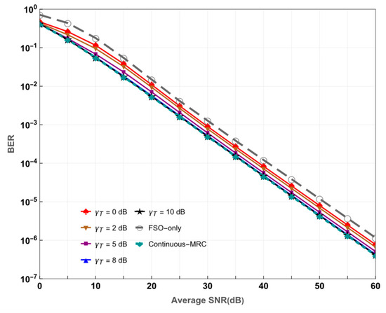
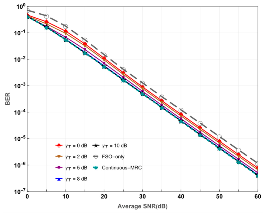
According to the activation rule, the probability that the RF branch is activated is $P_{\mathrm{a}\mathrm{c}\mathrm{t}}=\mathrm{P}\mathrm{r}\{{\gamma }_2^{\mathrm{F}\mathrm{S}\mathrm{O}}<{\gamma }_T\}=F_{{\gamma }_2^{\mathrm{F}\mathrm{S}\mathrm{O}}}\left({\gamma }_T\right)$, where $F_{{\gamma }_2^{\mathrm{F}\mathrm{S}\mathrm{O}}}(\cdot )$is given in (13). Therefore, increasing ${\gamma }_{T }$ increases the proportion of fading blocks processed by dual-branch MRC and tends to reduce the second-hop BER, approaching the continuous-MRC limit as ${\gamma }_T\to \infty$. However, it also increases the RF activation duty cycle, average RF energy consumption, and implementation overhead. Conversely, decreasing ${\gamma }_T$conserves RF resources but causes more impaired FSO blocks to be decoded without RF assistance. To explicitly examine this tradeoff, Figure 2 evaluates the end-to-end BER for ${\gamma }_{T,\mathrm{d}\mathrm{B}}=0, 2, 5, 8,$and $10 \mathrm{d}\mathrm{B}$, together with the FSO-only and continuous-MRC limiting cases. Accordingly, ${\gamma }_{T,\mathrm{d}\mathrm{B}}=5 \mathrm{d}\mathrm{B}$, which lies near the knee of the reliability–resource tradeoff observed in Figure 2, is adopted in Table 2 as a representative baseline operating point rather than being claimed as a universal optimum. For practical deployment, ${\gamma }_T$may be determined through a one-dimensional search using (34), subject to a prescribed RF activation constraint $P_{\mathrm{a}\mathrm{c}\mathrm{t}}\le {\eta }_{\mathrm{m}\mathrm{a}\mathrm{x}}$, where ${\eta }_{\mathrm{m}\mathrm{a}\mathrm{x}}$reflects the allowable RF duty cycle or average-energy budget.

Figure 2. End-to-end BER performance under different RF activation thresholds and the FSO-only and continuous-MRC limiting cases.

Table 2. Simulation parameters of the mixed FSO/RF links.

System Parameter	Symbol	Value	System Parameter	Symbol	Value
Laser wavelength	λ	1550 nm	RF carrier frequency	fRF	5 GHz
Satellite altitude	HS	3600 km	HAP altitude	HH	20 km
LOS phase difference	φA − φB	π/2	Shadowing parameter	m2	19.4
Scattering power	2 b0,2	0.158	Turbulence parameter	Cn2(0)	7.5 × 10−17
Switching threshold	γT	5 dB	Wind speed	v	21 m/s
LOS component power	Ω2	1.29	Constellation size	M	16
Transmit beam waist	ω0	0.1 m	Aperture diameter	D	0.2 m
Zenith angle	ζ	30°	RF average SNR	${\overline{\gamma }}_2^{\mathit{RF}}$	10 dB

Figure 2 compares the end-to-end BER for ${\gamma }_{T,\mathrm{d}\mathrm{B}}=0, 2, 5, 8,$ and $10 \mathrm{d}\mathrm{B}$, together with the FSO-only and continuous-MRC limiting cases. At a BER of ${10}^{-4}$, increasing ${\gamma }_{T,\mathrm{d}\mathrm{B}}$ from $0$ to $5 \mathrm{d}\mathrm{B}$ reduces the required average SNR from approximately $39.2$ to $37.6 \mathrm{d}\mathrm{B}$, whereas increasing it further from $5$ to $10 \mathrm{d}\mathrm{B}$ provides only about $0.8 \mathrm{d}\mathrm{B}$ of additional gain. This confirms the diminishing BER improvement at higher thresholds and supports $5 \mathrm{d}\mathrm{B}$ as a representative reliability–resource tradeoff point rather than a universal optimum.

It should be emphasized that the ${\gamma }_{T,\mathrm{d}\mathrm{B}}=0 \mathrm{d}\mathrm{B}$ curve represents a finite-threshold operating point and is not the FSO-only limit. Because ${\gamma }_T$in (29)–(34) is defined on a linear SNR scale, the FSO-only case is obtained for ${\gamma }_T=0$(or equivalently ${\gamma }_T\to 0^{+}$), corresponding to ${\gamma }_{T,\mathrm{d}\mathrm{B}}\to -\mathrm{\infty }$, for which $P_{\mathrm{a}\mathrm{c}\mathrm{t}}=0$. Conversely, as ${\gamma }_T\to \mathrm{\infty }$, $P_{\mathrm{a}\mathrm{c}\mathrm{t}}\to 1$, and the RF branch is continuously activated, yielding continuous two-branch MRC. The continuous-MRC case is a distinct limiting protocol with the RF branch always active and is not asymptotically equivalent to any fixed finite threshold.

Under the common high-SNR scaling adopted in Section 3 and the assumed independence of the FSO and RF branches, the FSO-only second hop has diversity order $d_2^{\mathrm{F}\mathrm{S}\mathrm{O}}$. Any fixed finite threshold retains the same diversity order because the RF activation probability vanishes as the average SNR tends to infinity, although the threshold changes the asymptotic coefficient and, over the examined range, improves the corresponding coding gain. In contrast, continuous MRC achieves diversity order $d_2^{\mathrm{F}\mathrm{S}\mathrm{O}}+1$, since the independent shadowed-Rician RF branch contributes first-order diversity. Hence, $d_{\mathrm{e}2\mathrm{e}}^{\mathrm{f}\mathrm{i}\mathrm{n}\mathrm{i}\mathrm{t}\mathrm{e}}=d_{\mathrm{e}2\mathrm{e}}^{FSO-only}=\mathrm{m}\mathrm{i}\mathrm{n}\left\{d_1,d_2^{\mathrm{F}\mathrm{S}\mathrm{O}},d_3\right\},$whereas $d_{\mathrm{e}2\mathrm{e}}^{\mathrm{c}\mathrm{o}\mathrm{n}\mathrm{t}\mathrm{i}\mathrm{n}\mathrm{u}\mathrm{o}\mathrm{u}\mathrm{s}-\mathrm{M}\mathrm{R}\mathrm{C}}=\mathrm{m}\mathrm{i}\mathrm{n}\left\{d_1,d_2^{\mathrm{F}\mathrm{S}\mathrm{O}}+1,d_3\right\}.$ Thus, continuous MRC increases the end-to-end diversity order only when $d_2^{\mathrm{F}\mathrm{S}\mathrm{O}}<\mathrm{m}\mathrm{i}\mathrm{n}\{d_1,d_3\}$; otherwise, another hop remains the diversity bottleneck.

$$f_{{\gamma }_2}(y)=\left\{\begin{array}{ll}{f}_{{\gamma }_2^{\mathrm{MRC}}}(y),\hfill & 0<y\le {\gamma }_T\hfill \\ G(y)+f_{{\gamma }_2^{\mathrm{FSO}}}(y),\hfill & y>{\gamma }_T\hfill \end{array}\right.$$

(29)

$$f_{{\gamma }_2^{\mathrm{MRC}}}(y)={\displaystyle {\int }_0^y{f}_{{\gamma }_2^{\mathrm{FSO}}}}(t)f_{{\gamma }_2^{\mathrm{RF}}}(y-t)dt$$

(30)

$$G(y)={\displaystyle {\int }_0^{{\gamma }_T}{f}_{{\gamma }_2^{\mathrm{FSO}}}}(t)f_{{\gamma }_2^{\mathrm{RF}}}(y-t)dt$$

(31)

To decouple the integration variables in (30) and (31), the binomial theorem, the Taylor-series expansion of the exponential function, and the infinite-series expansion of the confluent hypergeometric function ${}_{1}F_1\left(\cdot \right)$are employed. By substituting (12) and (18) into (30) and (31), and further using the integral identity (07.34.21.0003.01) given in [38], $f_{{\gamma }_2^{\mathrm{M}\mathrm{R}\mathrm{C}}}(y)$and $G\left(y\right)$can be respectively derived as follows:

$$\begin{array}{ll}{f}_{{\gamma }_2^{\mathrm{MRC}}}(\gamma )=& {\displaystyle \frac{{\xi }_{2,mod}^2{A}_2{\left(\frac{2b_{0,2}{m}_2}{2b_{0,2}{m}_2+{\Omega }_2}\right)}^{m_2}}{4b_{0,2}{\overline{\gamma }}_{rf,2}}}\exp \left(-{\displaystyle \frac{\gamma }{2b_{0,2}{\overline{\gamma }}_{rf,2}}}\right)\times {\displaystyle \sum _{k_2=0}^{\infty }{\displaystyle \sum _{j=0}^{k_2}{\displaystyle \sum _{k_3=0}^{\infty }\frac{\Gamma (m_2+k_2)}{\Gamma (m_2){(k_2!)}^2{k}_3!}}}}{\left({\displaystyle \frac{{\Omega }_2}{2b_{0,2}{\overline{\gamma }}_{rf,2}(2b_{0,2}{m}_2+{\Omega }_2)}}\right)}^{k_2}\\ & {\left({\displaystyle \frac{1}{2b_{0,2}{\overline{\gamma }}_{rf,2}}}\right)}^{k_3}\left(\begin{array}{c}{k}_2\\ j\end{array}\right){(-1)}^j{\gamma }^{k_2+k_3}\times {\displaystyle \sum _{m^{\prime }=1}^{{\beta }_2}{b}_{m^{\prime }}^{(2)}}{G}_{2,4}^{3,1}\left({\displaystyle \frac{B_2\gamma }{A_{2,mod}{\overline{\gamma }}_{fso,2}}}|\begin{array}{c}1-j-k_3,{\xi }_{2,mod}^2+1\\ {\xi }_{2,mod}^2,{\alpha }_2,m^{\prime },-j-k_3\end{array}\right)\end{array}$$

(32)

$$\begin{array}{ll}G(\gamma )=& {\displaystyle \frac{{\xi }_{2,mod}^2{A}_2{\left(\frac{2b_{0,2}{m}_2}{2b_{0,2}{m}_2+{\Omega }_2}\right)}^{m_2}}{4b_{0,2}{\overline{\gamma }}_{rf,2}}}\exp \left(-{\displaystyle \frac{\gamma }{2b_{0,2}{\overline{\gamma }}_{rf,2}}}\right)\times {\displaystyle \sum _{k_2=0}^{\infty }{\displaystyle \sum _{j=0}^{k_2}{\displaystyle \sum _{k_3=0}^{\infty }\frac{\Gamma (m_2+k_2)}{\Gamma (m_2){(k_2!)}^2{k}_3!}}}}{\left({\displaystyle \frac{{\Omega }_2}{2b_{0,2}{\overline{\gamma }}_{rf,2}(2b_{0,2}{m}_2+{\Omega }_2)}}\right)}^{k_2}{\left({\displaystyle \frac{1}{2b_{0,2}{\overline{\gamma }}_{rf,2}}}\right)}^{k_3}\\ & \left(\begin{array}{c}{k}_2\\ j\end{array}\right){(-1)}^j{\gamma }^{k_2-j}{\gamma }_T^{j+k_3}\times {\displaystyle \sum _{m^{\prime }=1}^{{\beta }_2}{b}_{m^{\prime }}^{(2)}}{G}_{2,4}^{3,1}\left({\displaystyle \frac{B_2{\gamma }_T}{A_{2,mod}{\overline{\gamma }}_{fso,2}}}|\begin{array}{c}1-j-k_3,{\xi }_{2,mod}^2+1\\ {\xi }_{2,mod}^2,{\alpha }_2,m^{\prime },-j-k_3\end{array}\right)\end{array}$$

(33)

On this basis, according to the definition of the average BER and by substituting the piecewise PDF of the second-hop output SNR, the average BER of the second-hop adaptive link can be expressed as

$${\overline{P}}_2=K_{CN}{\displaystyle {\int }_0^{{\gamma }_T}{f}_{{\gamma }_2^{\mathrm{MRC}}}}(y)Q(\sqrt{\tau y})dy+K_{CN}{\displaystyle {\int }_{{\gamma }_T}^{\infty }\left[G(y)+f_{{\gamma }_2^{\mathrm{FSO}}}(y)\right]}Q(\sqrt{\tau y})dy$$

(34)

Since the above integral expression is difficult to solve directly, the Gauss–Legendre and Gauss–Laguerre quadrature formulas are adopted to numerically approximate the finite interval $\left[0,{\gamma }_T\right]$ and the infinite interval [${\gamma }_T$, ∞), respectively. Let $x_m$ and $w_m$ denote the nodes and weights of the M-order Gauss–Legendre quadrature, respectively, and let ${\lambda }_n$ and ${\omega }_n$ denote the nodes and weights of the N-order Gauss–Laguerre quadrature, respectively. By applying variable transformations, the average BER of the second hop can be decomposed as $\overline{P_2}=\overline{P_{21}}+\overline{P_{22}}$. The corresponding approximate analytical expressions based on Gaussian quadrature are given as follows:

$$\begin{array}{ll}{\overline{P}}_{21}=& {\displaystyle \frac{{\gamma }_T{K}_{CN}{\xi }_{2,mod}^2{A}_2{\left(\frac{2b_{0,2}{m}_2}{2b_{0,2}{m}_2+{\Omega }_2}\right)}^{m_2}}{16\sqrt{\pi }{b}_{0,2}{\overline{\gamma }}_{rf,2}}}{\displaystyle {\displaystyle \sum _{m=1}^M}{w}_m}\exp \left(-{\displaystyle \frac{{\gamma }_T(x_m+1)}{4b_{0,2}{\overline{\gamma }}_{rf,2}}}\right)\times {\displaystyle {\displaystyle \sum _{k_2=0}^{\infty }}{\displaystyle \sum _{j=0}^{k_2}{\displaystyle \sum _{k_3=0}^{\infty }\frac{\Gamma (m_2+k_2)}{\Gamma (m_2){(k_2!)}^2{k}_3!}}}}\\ & {\left({\displaystyle \frac{{\Omega }_2}{2b_{0,2}{\overline{\gamma }}_{rf,2}(2b_{0,2}{m}_2+{\Omega }_2)}}\right)}^{k_2}{\left({\displaystyle \frac{1}{2b_{0,2}{\overline{\gamma }}_{rf,2}}}\right)}^{k_3}\left(\begin{array}{c}{k}_2\\ j\end{array}\right){(-1)}^j{\left({\displaystyle \frac{{\gamma }_T(x_m+1)}{2}}\right)}^{k_2+k_3}\times {\displaystyle \sum _{m^{\prime }=1}^{{\beta }_2}{b}_{m^{\prime }}^{(2)}}{G}_{2,4}^{3,1}\\ & \left({\displaystyle \frac{B_2{\gamma }_T(x_m+1)}{2A_{2,mod}{\overline{\gamma }}_{fso,2}}}|\begin{array}{c}1-j-k_3,{\xi }_{2,mod}^2+1\\ {\xi }_{2,mod}^2,{\alpha }_2,m^{\prime },-j-k_3\end{array}\right)G_{1,2}^{2,0}\left({\displaystyle \frac{\tau {\gamma }_T(x_m+1)}{4}}|\begin{array}{c}1\\ 0,{\displaystyle \frac{1}{2}}\end{array}\right)\end{array}$$

(35)

$$\begin{array}{ll}{\overline{P}}_{22}=& {\displaystyle \frac{K_{CN}{\xi }_{2,mod}^2{A}_2}{2\sqrt{\pi }}}{\displaystyle {\displaystyle \sum _{n=1}^N}{\omega }_n}{e}^{{\lambda }_n}\{{\displaystyle \frac{{\left(\frac{2b_{0,2}{m}_2}{2b_{0,2}{m}_2+{\Omega }_2}\right)}^{m_2}}{4b_{0,2}{\overline{\gamma }}_{rf,2}}}\exp \left(-{\displaystyle \frac{{\lambda }_n+{\gamma }_T}{2b_{0,2}{\overline{\gamma }}_{rf,2}}}\right)\times {\displaystyle {\displaystyle \sum _{k_2=0}^{\infty }}{\displaystyle \sum _{j=0}^{k_2}{\displaystyle \sum _{k_3=0}^{\infty }\frac{\Gamma (m_2+k_2)}{\Gamma (m_2){(k_2!)}^2{k}_3!}}}}{\left({\displaystyle \frac{{\Omega }_2}{2b_{0,2}{\overline{\gamma }}_{rf,2}(2b_{0,2}{m}_2+{\Omega }_2)}}\right)}^{k_2}\\ & {\left({\displaystyle \frac{1}{2b_{0,2}{\overline{\gamma }}_{rf,2}}}\right)}^{k_3}\left(\begin{array}{c}{k}_2\\ j\end{array}\right){(-1)}^j{({\lambda }_n+{\gamma }_T)}^{k_2-j}{\gamma }_T^{j+k_3}\times {\displaystyle \sum _{m^{\prime }=1}^{{\beta }_2}{b}_{m^{\prime }}^{(2)}}{G}_{2,4}^{3,1}\left({\displaystyle \frac{B_2{\gamma }_T}{A_{2,mod}{\overline{\gamma }}_{fso,2}}}|\begin{array}{c}1-j-k_3,{\xi }_{2,mod}^2+1\\ {\xi }_{2,mod}^2,{\alpha }_2,m^{\prime },-j-k_3\end{array}\right)+\\ & {\displaystyle \frac{1}{2({\lambda }_n+{\gamma }_T)}}{\displaystyle \sum _{m^{\prime }=1}^{{\beta }_2}{b}_{m^{\prime }}^{(2)}}{G}_{1,3}^{3,0}\left({\displaystyle \frac{B_2({\lambda }_n+{\gamma }_T)}{A_{2,mod}{\overline{\gamma }}_{fso,2}}}|\begin{array}{c}{\xi }_{2,mod}^2+1\\ {\xi }_{2,mod}^2,{\alpha }_2,m^{\prime }\end{array}\right)\}{G}_{1,2}^{2,0}\left({\displaystyle \frac{\tau ({\lambda }_n+{\gamma }_T)}{2}}|\begin{array}{c}1\\ 0,{\displaystyle \frac{1}{2}}\end{array}\right)\end{array}$$

(36)

where $w_m={\displaystyle \frac{2}{{\left(1-x_m\right)}^2{\left[P_M^{\prime }\left(x_m\right)\right]}^2}}$; the Legendre polynomial is given by $P_M\left(x\right)={\displaystyle \frac{1}{2^{M}M!}}{\displaystyle \frac{d^M}{d{x}^M}}{\left(x^2-1\right)}^M$. Similarly, ${\omega }_n={\displaystyle \frac{{\lambda }_n}{{\left(N+1\right)}^2{\left[L_{N+1}\left({\lambda }_n\right)\right]}^2}}$; the Laguerre polynomial is given by $L_N\left(x\right)={\displaystyle \frac{e^x}{N!}}{\displaystyle \frac{d^N}{d{x}^N}}\left(x^N{e}^{-x}\right)$.

$$\begin{array}{ll}{\overline{P}}_3=& {\displaystyle \frac{K_{CN}{\xi }_{3,mod}^2}{2\sqrt{\pi }}}[{\displaystyle \frac{{\omega }_3}{k_3{(2\pi )}^{\frac{k_3-1}{2}}}}{G}_{2k_3+1,k_3+2}^{2,2k_3}\left({\left({\displaystyle \frac{2k_3}{\tau A_{3,mod}{\lambda }_3{h}_3{\mu }_3}}\right)}^{k_3}|\begin{array}{c}\Delta (k_3,1),\Delta (k_3,{\displaystyle \frac{1}{2}}),{\displaystyle \frac{{\xi }_{3,mod}^2}{k_3}}+1\\ 1,{\displaystyle \frac{{\xi }_{3,mod}^2}{k_3}},\Delta (k_3,0)\end{array}\right)+\\ & {\displaystyle \frac{1-{\omega }_3}{\Gamma (a_3)c_3{(2\pi )}^{\frac{c_3-1}{2}}}}{G}_{2c_3+1,c_3+2}^{2,2c_3}\left({\left({\displaystyle \frac{2c_3}{\tau A_{3,mod}{b}_3{h}_3{\mu }_3}}\right)}^{c_3}|\begin{array}{c}\Delta (c_3,1),\Delta (c_3,{\displaystyle \frac{1}{2}}),{\displaystyle \frac{{\xi }_{3,mod}^2}{c_3}}+1\\ a_3,{\displaystyle \frac{{\xi }_{3,mod}^2}{c_3}},\Delta (c_3,0)\end{array}\right)]\end{array}$$

(37)

where $\mathsf{\Delta }\left(k,x\right)$ is defined as the parameter sequence $\mathsf{\Delta }\left(k,x\right)={\displaystyle \frac{x}{k}},{\displaystyle \frac{x+1}{k}},\dots ,{\displaystyle \frac{x+k-1}{k}}$.

By directly substituting the derived $\overline{P_1}$, $\overline{P_2}$ (where $\overline{P_2}=\overline{P_{21}}+\overline{P_{22}}$), and ${\overline{P}}_3$ into (23), the end-to-end average BER of the considered system can be obtained.

The analytical BER expressions are mainly intended for offline performance evaluation and system parameter selection. Let $K_2$and $K_3$denote the truncation orders of the infinite series indexed by $k_2$and $k_3$, respectively, and let $M$and $N$denote the Gauss–Legendre and Gauss–Laguerre quadrature orders. Since the inner index $j$ ranges from $0$to $k_2$, the number of truncated series terms at each quadrature node is ${ S}_{K_2,K_3}={\displaystyle {\sum }_{k_2=0}^{K_2}}\left(k_2+1\right)\left(K_3+1\right)={\displaystyle \frac{\left(K_2+1\right)\left(K_2+2\right)\left(K_3+1\right)}{2}}.$

Considering the finite summation associated with the Málaga-$ℳ$ parameter ${\mathsf{\beta }}_2$, the dominant computational cost for evaluating one average SNR point is proportional to ${\mathsf{\beta }}_2\left(\mathrm{M}+\mathrm{N}\right){\mathrm{S}}_{{\mathrm{K}}_2,{\mathrm{K}}_3}$, corresponding asymptotically to $\mathcal{O}\hspace{0.17em}\left({\mathsf{\beta }}_2\left(\mathrm{M}+\mathrm{N}\right){\mathrm{K}}_2^2{\mathrm{K}}_3\right)$special function evaluations. The numerical cost is mainly determined by the evaluation of the Meijer-$\mathrm{G}$ functions. The truncation and quadrature orders can be increased until the relative change in the calculated BER falls below a prescribed tolerance.

Importantly, these analytical series, quadratures, and Meijer-$G$ functions are evaluated only for offline performance analysis. For a fixed two-branch receiver, online implementation requires FSO-SNR estimation and one threshold comparison; when the threshold condition is satisfied, RF-channel estimation, RF-branch activation, and two-branch MRC are additionally performed. Therefore, the online decision and combining complexity is $\mathcal{O}\left(1\right)$with respect to $K_2$, $K_3$, $M$, and $N$, although channel estimation, synchronization, and RF-chain activation still introduce practical overhead.

As $\rho \to \infty$, the average-SNR-dependent arguments of the Meijer-$G$ functions in (28) and (35)–(37) approach zero. By applying the small-argument expansion of the Meijer-$G$ function given in [38], Equation (07.34.06.0001.01) and retaining the leading residue terms, the asymptotic average BER of the first-hop satellite-to-HAP FSO link is obtained as

$$\begin{array}{l}{\overline{P}}_1^{\mathrm{asy}}={\displaystyle \frac{K_{CN}{\xi }_{1,\mathrm{mod}}^2{A}_1}{4\sqrt{\pi }}}{\displaystyle \sum _{m^{\prime }=1}^{{\beta }_1}{b}_{m^{\prime }}^{(1)}}[{\displaystyle \frac{\Gamma ({\alpha }_1-{\xi }_{1,\mathrm{mod}}^2)\Gamma (m^{\prime }-{\xi }_{1,\mathrm{mod}}^2)\Gamma ({\xi }_{1,\mathrm{mod}}^2)\Gamma \left({\xi }_{1,\mathrm{mod}}^2+\frac{1}{2}\right)}{\Gamma (1+{\xi }_{1,\mathrm{mod}}^2)}}{\left({\displaystyle \frac{2B_1}{\tau A_{1,\mathrm{mod}}{\overline{\gamma }}_1}}\right)}^{{\xi }_{1,\mathrm{mod}}^2}\\ +{\displaystyle \frac{\Gamma ({\xi }_{1,\mathrm{mod}}^2-{\alpha }_1)\Gamma (m^{\prime }-{\alpha }_1)\Gamma ({\alpha }_1)\Gamma \left({\alpha }_1+\frac{1}{2}\right)}{\Gamma ({\xi }_{1,\mathrm{mod}}^2+1-{\alpha }_1)\Gamma (1+{\alpha }_1)}}{\left({\displaystyle \frac{2B_1}{\tau A_{1,\mathrm{mod}}{\overline{\gamma }}_1}}\right)}^{{\alpha }_1}+{\displaystyle \frac{\Gamma ({\xi }_{1,\mathrm{mod}}^2-m^{\prime })\Gamma ({\alpha }_1-m^{\prime })\Gamma (m^{\prime })\Gamma \left(m^{\prime }+\frac{1}{2}\right)}{\Gamma ({\xi }_{1,\mathrm{mod}}^2+1-m^{\prime })\Gamma (1+m^{\prime })}}{\left({\displaystyle \frac{2B_1}{\tau A_{1,\mathrm{mod}}{\overline{\gamma }}_1}}\right)}^{m^{\prime }}]\end{array}$$

(38)

For the adaptive mixed FSO/RF second hop, the asymptotic average BER can first be decomposed as

$${\overline{P}}_2^{\mathrm{a}\mathrm{s}\mathrm{y}}={\overline{P}}_{21}^{\mathrm{a}\mathrm{s}\mathrm{y}}+{\overline{P}}_{22}^{\mathrm{a}\mathrm{s}\mathrm{y}}$$

(39)

Applying the same small-argument Meijer-$G$ expansion in [38], Equation (07.34.06.0001.01) to the two BER components in (35) and (36), and retaining their leading residue terms, gives, respectively,

$$\begin{array}{l}{\overline{P}}_{21}^{\mathrm{asy}}={\displaystyle \frac{{\gamma }_T{K}_{CN}{\xi }_{2,\mathrm{mod}}^2{A}_2}{16\sqrt{\pi }{b}_{0,2}{\overline{\gamma }}_{\mathrm{rf},2}}}{\left({\displaystyle \frac{2b_{0,2}{m}_2}{2b_{0,2}{m}_2+{\Omega }_2}}\right)}^{m_2}{\displaystyle \sum _{m=1}^M{w}_m}\exp \left[-{\displaystyle \frac{{\gamma }_T(x_m+1)}{4b_{0,2}{\overline{\gamma }}_{\mathrm{rf},2}}}\right]\times \\ {\displaystyle \sum _{k_2=0}^{\infty }{\displaystyle \sum _{j=0}^{k_2}{\displaystyle \sum _{k_3=0}^{\infty }\frac{\Gamma (m_2+k_2)}{\Gamma (m_2){(k_2!)}^2{k}_3!}}}}{\left[{\displaystyle \frac{{\Omega }_2}{2b_{0,2}{\overline{\gamma }}_{\mathrm{rf},2}(2b_{0,2}{m}_2+{\Omega }_2)}}\right]}^{k_2}{\left({\displaystyle \frac{1}{2b_{0,2}{\overline{\gamma }}_{\mathrm{rf},2}}}\right)}^{k_3}\left(\begin{array}{c}{k}_2\\ j\end{array}\right){(-1)}^j{\left[{\displaystyle \frac{{\gamma }_T(x_m+1)}{2}}\right]}^{k_2+k_3}\\ \times {\displaystyle \sum _{m^{\prime }=1}^{{\beta }_2}{b}_{m^{\prime }}^{(2)}}[{\displaystyle \frac{\Gamma ({\alpha }_2-{\xi }_{2,\mathrm{mod}}^2)\Gamma (m^{\prime }-{\xi }_{2,\mathrm{mod}}^2)}{j+k_3+{\xi }_{2,\mathrm{mod}}^2}}{\left[{\displaystyle \frac{B_2{\gamma }_T(x_m+1)}{2A_{2,\mathrm{mod}}{\overline{\gamma }}_{\mathrm{fso},2}}}\right]}^{{\xi }_{2,\mathrm{mod}}^2}+{\displaystyle \frac{\Gamma ({\xi }_{2,\mathrm{mod}}^2-{\alpha }_2)\Gamma (m^{\prime }-{\alpha }_2)}{\Gamma ({\xi }_{2,\mathrm{mod}}^2+1-{\alpha }_2)(j+k_3+{\alpha }_2)}}{\left[{\displaystyle \frac{B_2{\gamma }_T(x_m+1)}{2A_{2,\mathrm{mod}}{\overline{\gamma }}_{\mathrm{fso},2}}}\right]}^{{\alpha }_2}\\ +{\displaystyle \frac{\Gamma ({\xi }_{2,\mathrm{mod}}^2-m^{\prime })\Gamma ({\alpha }_2-m^{\prime })}{\Gamma ({\xi }_{2,\mathrm{mod}}^2+1-m^{\prime })(j+k_3+m^{\prime })}}{\left[{\displaystyle \frac{B_2{\gamma }_T(x_m+1)}{2A_{2,\mathrm{mod}}{\overline{\gamma }}_{\mathrm{fso},2}}}\right]}^{m^{\prime }}]\times G_{1,2}^{2,0}\left({\displaystyle \frac{\tau {\gamma }_T(x_m+1)}{4}}\left|\begin{array}{c}1\\ 0,{\displaystyle \frac{1}{2}}\end{array}\right.\right)\end{array}$$

(40)

$$\begin{array}{l}{\overline{P}}_{22}^{\mathrm{asy}}={\displaystyle \frac{K_{CN}{\xi }_{2,\mathrm{mod}}^2{A}_2}{2\sqrt{\pi }}}{\displaystyle \sum _{n=1}^N{\omega }_n}{e}^{{\lambda }_n}\{{\displaystyle \frac{1}{4b_{0,2}{\overline{\gamma }}_{\mathrm{rf},2}}}{\left({\displaystyle \frac{2b_{0,2}{m}_2}{2b_{0,2}{m}_2+{\Omega }_2}}\right)}^{m_2}\exp \left[-{\displaystyle \frac{{\lambda }_n+{\gamma }_T}{2b_{0,2}{\overline{\gamma }}_{\mathrm{rf},2}}}\right]\times \\ {\displaystyle \sum _{k_2=0}^{\infty }{\displaystyle \sum _{j=0}^{k_2}{\displaystyle \sum _{k_3=0}^{\infty }\frac{\Gamma (m_2+k_2)}{\Gamma (m_2){(k_2!)}^2{k}_3!}}}}{\left[{\displaystyle \frac{{\Omega }_2}{2b_{0,2}{\overline{\gamma }}_{\mathrm{rf},2}(2b_{0,2}{m}_2+{\Omega }_2)}}\right]}^{k_2}{\left({\displaystyle \frac{1}{2b_{0,2}{\overline{\gamma }}_{\mathrm{rf},2}}}\right)}^{k_3}\left(\begin{array}{c}{k}_2\\ j\end{array}\right){(-1)}^j{({\lambda }_n+{\gamma }_T)}^{k_2-j}{\gamma }_T^{j+k_3}\times \\ {\displaystyle \sum _{m^{\prime }=1}^{{\beta }_2}{b}_{m^{\prime }}^{(2)}}[{\displaystyle \frac{\Gamma ({\alpha }_2-{\xi }_{2,\mathrm{mod}}^2)\Gamma (m^{\prime }-{\xi }_{2,\mathrm{mod}}^2)}{j+k_3+{\xi }_{2,\mathrm{mod}}^2}}{\left[{\displaystyle \frac{B_2{\gamma }_T}{A_{2,\mathrm{mod}}{\overline{\gamma }}_{\mathrm{fso},2}}}\right]}^{{\xi }_{2,\mathrm{mod}}^2}+{\displaystyle \frac{\Gamma ({\xi }_{2,\mathrm{mod}}^2-{\alpha }_2)\Gamma (m^{\prime }-{\alpha }_2)}{\Gamma ({\xi }_{2,\mathrm{mod}}^2+1-{\alpha }_2)(j+k_3+{\alpha }_2)}}{\left[{\displaystyle \frac{B_2{\gamma }_T}{A_{2,\mathrm{mod}}{\overline{\gamma }}_{\mathrm{fso},2}}}\right]}^{{\alpha }_2}\\ +{\displaystyle \frac{\Gamma ({\xi }_{2,\mathrm{mod}}^2-m^{\prime })\Gamma ({\alpha }_2-m^{\prime })}{\Gamma ({\xi }_{2,\mathrm{mod}}^2+1-m^{\prime })(j+k_3+m^{\prime })}}{\left[{\displaystyle \frac{B_2{\gamma }_T}{A_{2,\mathrm{mod}}{\overline{\gamma }}_{\mathrm{fso},2}}}\right]}^{m^{\prime }}]+{\displaystyle \frac{1}{2({\lambda }_n+{\gamma }_T)}}{\displaystyle \sum _{m^{\prime }=1}^{{\beta }_2}{b}_{m^{\prime }}^{(2)}}[\Gamma ({\alpha }_2-{\xi }_{2,\mathrm{mod}}^2)\Gamma (m^{\prime }-{\xi }_{2,\mathrm{mod}}^2){\left[{\displaystyle \frac{B_2({\lambda }_n+{\gamma }_T)}{A_{2,\mathrm{mod}}{\overline{\gamma }}_{\mathrm{fso},2}}}\right]}^{{\xi }_{2,\mathrm{mod}}^2}\\ +{\displaystyle \frac{\Gamma ({\xi }_{2,\mathrm{mod}}^2-{\alpha }_2)\Gamma (m^{\prime }-{\alpha }_2)}{\Gamma ({\xi }_{2,\mathrm{mod}}^2+1-{\alpha }_2)}}{\left[{\displaystyle \frac{B_2({\lambda }_n+{\gamma }_T)}{A_{2,\mathrm{mod}}{\overline{\gamma }}_{\mathrm{fso},2}}}\right]}^{{\alpha }_2}+{\displaystyle \frac{\Gamma ({\xi }_{2,\mathrm{mod}}^2-m^{\prime })\Gamma ({\alpha }_2-m^{\prime })}{\Gamma ({\xi }_{2,\mathrm{mod}}^2+1-m^{\prime })}}{\left[{\displaystyle \frac{B_2({\lambda }_n+{\gamma }_T)}{A_{2,\mathrm{mod}}{\overline{\gamma }}_{\mathrm{fso},2}}}\right]}^{m^{\prime }}]\}\times G_{1,2}^{2,0}\left({\displaystyle \frac{\tau ({\lambda }_n+{\gamma }_T)}{2}}\left|\begin{array}{c}1\\ 0,{\displaystyle \frac{1}{2}}\end{array}\right.\right)\end{array}$$

(41)

For any fixed finite activation threshold, the RF-assisted contributions contain an additional inverse RF-SNR factor relative to the FSO-only contribution. Consequently, the threshold changes the dominant asymptotic coefficient and, hence, the coding gain, but it does not change the second-hop diversity order.

For the third-hop UWOC link, applying the small-argument series expansion of the Meijer-$G$ function in [38], Equation (07.34.06.0001.01) to the representation in (22) and retaining the dominant near-zero power terms yields the following asymptotic expressions for the two WGG mixture components:

$${\overline{P}}_3^{\hspace{0.17em}\mathrm{a}\mathrm{s}\mathrm{y}}={\overline{P}}_{3,\mathrm{W}}^{\hspace{0.17em}\mathrm{a}\mathrm{s}\mathrm{y}}+{\overline{P}}_{3,\mathrm{G}}^{\hspace{0.17em}\mathrm{a}\mathrm{s}\mathrm{y}}$$

(42)

For the Weibull component, the turbulence term dominates when the Weibull exponent is smaller than the pointing-error exponent, yielding

$${\overline{P}}_{3,\mathrm{W}}^{\hspace{0.17em}\mathrm{a}\mathrm{s}\mathrm{y}}={\displaystyle \frac{K_{CN}{2}^{\frac{k_3}{R_3}-1}\Gamma \left(\frac{k_3}{R_3}+\frac{1}{2}\right)}{\sqrt{\pi }\hspace{0.17em}{\tau }^{\frac{k_3}{R_3}}}}{\displaystyle \frac{{\omega }_3{\xi }_{3,\mathrm{m}\mathrm{o}\mathrm{d}}^2}{{\xi }_{3,\mathrm{m}\mathrm{o}\mathrm{d}}^2-k_3}}{\displaystyle \frac{{\mu }_3^{-\frac{k_3}{R_3}}}{{\left(A_{3,\mathrm{m}\mathrm{o}\mathrm{d}}{\lambda }_3{h}_3\right)}^{k_3}}} ,\hspace{1em}\hspace{1em}{k}_3<{\xi }_{3,\mathrm{m}\mathrm{o}\mathrm{d}}^2$$

(43a)

When the pointing-error exponent is smaller than the Weibull exponent, the corresponding dominant term is

$${\overline{P}}_{3,\mathrm{W}}^{\hspace{0.17em}\mathrm{a}\mathrm{s}\mathrm{y}}={\displaystyle \frac{K_{CN}{2}^{\frac{{\xi }_{3,\mathrm{m}\mathrm{o}\mathrm{d}}^2}{R_3}-1}\Gamma \left(\frac{{\xi }_{3,\mathrm{m}\mathrm{o}\mathrm{d}}^2}{R_3}+\frac{1}{2}\right)}{\sqrt{\pi }\hspace{0.17em}{\tau }^{\frac{{\xi }_{3,\mathrm{m}\mathrm{o}\mathrm{d}}^2}{R_3}}}}{\omega }_3\Gamma \left(1-{\displaystyle \frac{{\xi }_{3,\mathrm{m}\mathrm{o}\mathrm{d}}^2}{k_3}}\right){\displaystyle \frac{{\mu }_3^{-\frac{{\xi }_{3,\mathrm{m}\mathrm{o}\mathrm{d}}^2}{R_3}}}{{\left(A_{3,\mathrm{m}\mathrm{o}\mathrm{d}}{\lambda }_3{h}_3\right)}^{{\xi }_{3,\mathrm{m}\mathrm{o}\mathrm{d}}^2}}}$$

(43b)

For the generalized-Gamma component, the turbulence term dominates when its low-end exponent is smaller than the pointing-error exponent, yielding

$${\overline{P}}_{3,\mathrm{G}}^{\hspace{0.17em}\mathrm{a}\mathrm{s}\mathrm{y}}={\displaystyle \frac{K_{CN}{2}^{\frac{a_3{c}_3}{R_3}-1}\Gamma \left(\frac{a_3{c}_3}{R_3}+\frac{1}{2}\right)}{\sqrt{\pi }\hspace{0.17em}{\tau }^{\frac{a_3{c}_3}{R_3}}}}{\displaystyle \frac{\left(1-{\omega }_3\right){\xi }_{3,\mathrm{m}\mathrm{o}\mathrm{d}}^2}{a_3\Gamma \left(a_3\right)\left({\xi }_{3,\mathrm{m}\mathrm{o}\mathrm{d}}^2-a_3{c}_3\right)}}{\displaystyle \frac{{\mu }_3^{-\frac{a_3{c}_3}{R_3}}}{{\left(A_{3,\mathrm{m}\mathrm{o}\mathrm{d}}{b}_3{h}_3\right)}^{a_3{c}_3}}} ,\hspace{1em}\hspace{1em}{a}_3{c}_3<{\xi }_{3,\mathrm{m}\mathrm{o}\mathrm{d}}^2$$

(44a)

When ${\xi }_{3,\mathrm{m}\mathrm{o}\mathrm{d}}^2<a_3{c}_3$, the pointing-error term controls the generalized-Gamma component, yielding

$${\overline{P}}_{3,\mathrm{G}}^{\hspace{0.17em}\mathrm{a}\mathrm{s}\mathrm{y}}={\displaystyle \frac{K_{CN}{2}^{\frac{{\xi }_{3,\mathrm{m}\mathrm{o}\mathrm{d}}^2}{R_3}-1}\Gamma \left(\frac{{\xi }_{3,\mathrm{m}\mathrm{o}\mathrm{d}}^2}{R_3}+\frac{1}{2}\right)}{\sqrt{\pi }\hspace{0.17em}{\tau }^{\frac{{\xi }_{3,\mathrm{m}\mathrm{o}\mathrm{d}}^2}{R_3}}}}{\displaystyle \frac{\left(1-{\omega }_3\right)\Gamma \left(a_3-\frac{{\xi }_{3,\mathrm{m}\mathrm{o}\mathrm{d}}^2}{c_3}\right)}{\Gamma \left(a_3\right)}}{\displaystyle \frac{{\mu }_3^{-\frac{{\xi }_{3,\mathrm{m}\mathrm{o}\mathrm{d}}^2}{R_3}}}{{\left(A_{3,\mathrm{m}\mathrm{o}\mathrm{d}}{b}_3{h}_3\right)}^{{\xi }_{3,\mathrm{m}\mathrm{o}\mathrm{d}}^2}}},\hspace{1em}\hspace{1em}{\xi }_{3,\mathrm{m}\mathrm{o}\mathrm{d}}^2<a_3{c}_3$$

(44b)

Equations (43a)–(44b) assume noncoincident dominant exponents, i.e., $k_3\ne {\xi }_{3,\mathrm{m}\mathrm{o}\mathrm{d}}^2$ and $a_3{c}_3\ne {\xi }_{3,\mathrm{m}\mathrm{o}\mathrm{d}}^2$. The coincident cases can be obtained through the corresponding limiting procedure and are not encountered in the parameter sets considered in this paper.

Accordingly, the three per-hop diversity orders are

$$d_1=\mathrm{m}\mathrm{i}\mathrm{n}\left\{{\xi }_{1,\mathrm{m}\mathrm{o}\mathrm{d}}^2,{\alpha }_1,{\beta }_1\right\}$$

(45a)

$$d_2=\mathrm{m}\mathrm{i}\mathrm{n}\left\{{\xi }_{2,\mathrm{m}\mathrm{o}\mathrm{d}}^2,{\alpha }_2,{\beta }_2\right\}$$

(45b)

$$d_3=\mathrm{m}\mathrm{i}\mathrm{n}\left\{{\displaystyle \frac{k_3}{R_3}},{\displaystyle \frac{{\xi }_{3,\mathrm{m}\mathrm{o}\mathrm{d}}^2}{R_3}},{\displaystyle \frac{a_3{c}_3}{R_3}}\right\}$$

(45c)

Substituting (38), (40)–(42) into the exact three-hop DF BER relation in (23) gives the following composite high-SNR approximation, in which the DF cross-product terms are retained:

$$\begin{array}{ll}{\overline{P}}_{\mathrm{total}}^{\mathrm{DF},\mathrm{asy}}=& {\overline{P}}_1^{\mathrm{asy}}+{\overline{P}}_{21}^{\mathrm{asy}}+{\overline{P}}_{22}^{\mathrm{asy}}+{\overline{P}}_3^{\mathrm{asy}}-2{\overline{P}}_1^{\mathrm{asy}}\left({\overline{P}}_{21}^{\mathrm{asy}}+{\overline{P}}_{22}^{\mathrm{asy}}\right)-\\ & 2{\overline{P}}_1^{\mathrm{asy}}{\overline{P}}_3^{\mathrm{asy}}-2\left({\overline{P}}_{21}^{\mathrm{asy}}+{\overline{P}}_{22}^{\mathrm{asy}}\right){\overline{P}}_3^{\mathrm{asy}}+4{\overline{P}}_1^{\mathrm{asy}}\left({\overline{P}}_{21}^{\mathrm{asy}}+{\overline{P}}_{22}^{\mathrm{asy}}\right){\overline{P}}_3^{\mathrm{asy}}\end{array}$$

(46)

Because all second- and third-order BER product terms decay faster than the individual-hop terms as the average SNR tends to infinity, a first-order high-SNR approximation, obtained by neglecting the higher-order BER product terms, reduces to

$${\overline{P}}_{\mathrm{total}}^{\mathrm{DF}}\underset{\rho \to \infty }{~}{\overline{P}}_1^{\mathrm{asy}}+{\overline{P}}_{21}^{\mathrm{asy}}+{\overline{P}}_{22}^{\mathrm{asy}}+{\overline{P}}_3^{\mathrm{asy}}$$

(47)

Therefore, the end-to-end diversity order is

$$d_{\mathrm{e}2\mathrm{e}}=\mathrm{m}\mathrm{i}\mathrm{n}\left\{d_1,d_2,d_3\right\}$$

(48)

Writing the leading asymptotic BER of the $i$-th hop as ${\stackrel{-}{P}}_i^{\mathrm{a}\mathrm{s}\mathrm{y}}\sim C_i{\rho }^{-d_i}$, the strict dominant end-to-end form, the corresponding dominant coefficient, and the coding gain are given by

$$\begin{array}{l}{\overline{P}}_{\mathrm{t}\mathrm{o}\mathrm{t}\mathrm{a}\mathrm{l}}^{\mathrm{D}\mathrm{F}}\underset{\rho \to \infty }{\sim }{C}_{\mathrm{e}2\mathrm{e}}{\rho }^{-d_{\mathrm{e}2\mathrm{e}}}={\left(G_c\rho \right)}^{-d_{\mathrm{e}2\mathrm{e}}}\\ C_{\mathrm{e}2\mathrm{e}}={\displaystyle \sum _{i\in {\mathcal{L}}_{\mathrm{m}\mathrm{i}\mathrm{n}}}}{C}_i,\hspace{1em}\hspace{1em}{\mathcal{L}}_{\mathrm{m}\mathrm{i}\mathrm{n}}=\left\{i\in \left\{\mathrm{1,2},3\right\}\mid d_i=d_{\mathrm{e}2\mathrm{e}}\right\},\\ G_c=C_{\mathrm{e}2\mathrm{e}}^{-1/d_{\mathrm{e}2\mathrm{e}}}\end{array}$$

(49)

Thus, the smallest per-hop diversity order determines the high-SNR slope. If several hops attain the same minimum order, their leading asymptotic coefficients jointly determine the coding gain.

4. Simulation Analysis

Based on the above theoretical analysis and formula derivations, under the channel models of the Málaga-$ℳ$ distribution for the first hop, the shadowed-Rician fading distribution for the second hop, and the WGG distribution for the third hop, Monte Carlo simulations are conducted to verify the end-to-end transmission performance of the three-hop heterogeneous space–air–sea communication system employing the DF protocol. The simulation results validate the correctness of the derived analytical expressions for the end-to-end BER and illustrate the asymptotic behavior of the system in the high-SNR region. On this basis, the effects of key factors such as underwater turbulence, nonzero-boresight pointing errors, modulation schemes, underwater transmission distance, and shadowed fading on the system BER performance are further investigated. The detailed simulation parameters are listed in Table 2 and Table 3, where the mixed FSO/RF link parameters are mainly taken from [6,7,32], while the WGG distribution parameters of the UWOC link are mainly taken from [34].

Table 3. Turbulence parameters of the WGG distribution for the UWOC link.

GT (°C/cm)	GS (g/(L·cm))	RA (L/min)	σI2	(ω3, k3, λ3, a3, b3, c3)
0.1	0.05	5	0.3571	(0.2676, 2.1737, 0.3609, 72.4188, 1×10−6, 0.3053)
0.2	0.20	2	0.6725	(0.4200, 1.6400, 0.2870, 69.8487, 1.0248×10−6, 0.2974)
0.2	0.20	5	1.7670	(0.3150, 2.6702, 3.1768, 0.1755, 0.5155, 4.3411)

For clarity, Table 4 summarizes the physical meanings and units or dimensions of the principal system and channel parameters. Unless otherwise stated, normalized channel gains, noise powers, fading parameters, SNRs, and probabilities are dimensionless.

Table 4. Principal symbols and their units or dimensions.

Category	Symbol(s)	Physical Meaning	Unit/Dimension
Link parameters	$P_S,P_H,P_B;d_{SH},d_{HB},d_{BU}$	Transmit powers and hop distances	W; m or km
Receiver parameters	${\eta }_1, { \eta }_2,{ \eta }_3{; \sigma }_H^2,{\left({\sigma }_B^{FSO}\right)}^2, {\left({\sigma }_B^{RF}\right)}^2,{\sigma }_U^2$	Conversion factors and receiver-noise powers	A/W; dimensionless
Channel gains	$h_{SH},h_{HB}^{FSO},h_{BU}{;h}_{HB}^{RF},{\left|h_{HB}^{RF}\right|}^2$	Optical irradiance gains; RF amplitude and power gains	Dimensionless
SNR and detection	${\gamma }_i,{\overline{\gamma }}_i,{\gamma }_T;R_i$	Instantaneous/average SNR, threshold, and detection exponent	Dimensionless; dB when plotted
Pointing and geometry	${\mu }_{x,i},{\mu }_{y,i},{\sigma }_{x,i},{\sigma }_{y,i}{;w}_{eq,i},w_0,D,a$	Boresight, jitter, beamwidth, and aperture parameters	m; normalized ratios are dimensionless
Atmospheric quantities	$\lambda ,f_{RF},H_S,H_H,C_n^2,v,\zeta$	Wavelength, RF frequency, altitudes, turbulence strength, wind speed, and zenith angle	m; Hz; m;${ m}^{-2/3}$; m/s; rad
Atmospheric/RF fading	${\alpha }_i,{\beta }_i,g_i,{\Omega }_i\prime {;m}_2,2b_{\mathrm{0,2}},{\Omega }_2$	Málaga-$ℳ$ and shadowed-Rician parameters	Dimensionless
WGG parameters	${\omega }_3,k_3,{\lambda }_3,a_3,b_3,c_3,{\sigma }_I^2;G_T,G_S,R_A$	WGG channel and experimental parameters	Dimensionless; °C/cm; g/(L·cm); L/min
Performance/numerical	${\bar{P}}_1,{\bar{P}}_2,{\bar{P}}_3,{\bar{P}}_{\mathrm{t}\mathrm{o}\mathrm{t}\mathrm{a}\mathrm{l}}^{\mathrm{D}\mathrm{F}},P_{\mathrm{a}\mathrm{c}\mathrm{t}};K_2,K_3,M,N$	BERs, RF activation probability, truncation orders, and quadrature orders	Dimensionless probabilities; integers

The parameter sets in Table 2 and Table 3 are literature-based benchmarks selected to represent a plausible satellite–HAP–buoy–AUV configuration rather than measurements from a single deployment site. The satellite altitude of $3600 \mathrm{k}\mathrm{m}$ lies within the medium Earth orbit (MEO) regime, while an altitude of $20 \mathrm{k}\mathrm{m}$ is representative of a stratospheric HAP. The $1550 \mathrm{n}\mathrm{m}$ wavelength supports high-capacity FSO transmission, whereas the $5 \mathrm{G}\mathrm{H}\mathrm{z}$ RF branch is comparatively less sensitive to fog- and cloud-induced attenuation and, therefore, serves as a backup when the FSO branch is impaired [6,7]. The Málaga-$ℳ$ parameters $\left({\alpha }_i,\hspace{0.33em}{\beta }_i\right)=\left(2.296,\hspace{0.33em}2\right)$ provide a representative atmospheric turbulence benchmark [30], while the wind speed $v=21 \mathrm{m}/\mathrm{s}$ and the ground-level refractive index structure parameter $C_n^2\left(0\right)=7.5\times {10}^{-17} {\mathrm{m}}^{-2/3}$ specify the adopted reference atmospheric turbulence profile [6,7]. For the RF branch, the baseline shadowed-Rician tuple $\left(m_2,\hspace{0.33em}2b_{\mathrm{0,2}},\hspace{0.33em}{\mathsf{\Omega }}_2\right)=\left(19.4,\hspace{0.33em}0.158,\hspace{0.33em}1.29\right)$ represents infrequent light shadowing, where $m_2$ controls the LOS shadowing severity, $2b_{\mathrm{0,2}}$ denotes the average diffuse multipath power, and ${\mathsf{\Omega }}_2$ denotes the average LOS power [32]. The moderate- and heavy-shadowing cases considered in the numerical results are included as sensitivity benchmarks. The boresight displacement and jitter parameters are normalized by the receiver-aperture radius $a$, allowing rescaling for different terminal sizes [29]. The WGG parameter sets are fitted to measured thermocline and bubble conditions spanning different temperature gradients, salinity gradients, and air-bubble flow rates [34]. Accordingly, site-specific deployment requires recalibration using the actual orbit geometry, atmospheric profile, HAP station-keeping accuracy, sea state, water type, and AUV operating depth.

The two FSO links use the Málaga-$ℳ$ parameters ${\mathsf{\alpha }}_1={\mathsf{\alpha }}_2=2.296$, ${\mathsf{\beta }}_1={\mathsf{\beta }}_2=2$, ${\mathrm{g}}_1={\mathrm{g}}_2=0.087$, and ${\mathsf{\Omega }}_1^{\prime }={\mathsf{\Omega }}_2^{\prime }=1.455$. The baseline normalized pointing-error parameters are $\left({\mathsf{\mu }}_{\mathrm{x}}/\mathrm{a},{\mathsf{\mu }}_{\mathrm{y}}/\mathrm{a})=(\mathrm{1,2}\right)$ and $\left({\mathsf{\sigma }}_{\mathrm{x}}/\mathrm{a},{\mathsf{\sigma }}_{\mathrm{y}}/\mathrm{a})=(\mathrm{2,1}\right)$. The shadowed-Rician and WGG parameter sets are provided in Table 2 and Table 3, respectively, and the considered UWOC distances are $10$, $30$, $50$, and $70 \mathrm{m}$. The UWOC link employs HD or IM/DD, as indicated in each figure.

The numerical study is conducted in the normalized average electrical SNR domain. The relevant channel parameters are summarized in Table 2 and Table 3, while the deterministic link-budget and receiver parameters are incorporated into the corresponding average electrical SNR scales rather than treated as independent simulation variables. For Equations (32)–(36), the series truncation orders are $K_2=K_3=30$, and the Gauss–Legendre and Gauss–Laguerre quadrature orders are $M=N=40$, with relative and absolute tolerances of ${10}^{-6}$and ${10}^{-12}$, respectively. Numerical averaging uses four independently scrambled Sobol replicates, each containing $2^{20 }$samples, with the base seed 20260722. Independent conditional-average Monte Carlo simulations use seed 20261722, batches of $5\times {10}^5$samples, ${10}^6$–$4\times {10}^6$ samples per SNR point, and a $2\%$relative standard error stopping criterion. The Málaga-$ℳ$, shadowed-Rician, WGG, and pointing-error random variables are generated according to the corresponding channel models defined in Section 2. A concise overview of the Monte Carlo generation and BER evaluation procedure is provided in Algorithm 1.

Algorithm 1. Monte Carlo channel generation and BER evaluation.

Require: Channel and pointing-error parameters, SNR range, switching threshold, random seeds, sample limits, and tolerance. Ensure: End-to-end BER results and Monte Carlo verification.

1: Initialize the numerical settings and the sampling sequences used for numerical averaging and independent Monte Carlo verification. 2: Generate the Málaga-$ℳ$ atmospheric-fading samples from large-scale, coherent, and diffuse components using the normalized construction                 $I_{\mathcal{M},i}={\displaystyle \frac{X_i{\left|\sqrt{{\mathsf{\Omega }}_i\prime U_i}+Z_i\right|}^2}{{\mathsf{\Omega }}_i\prime +g_i}}$  where $X_i$and $U_i$are Gamma-distributed components, and $Z_i$is a diffuse complex Gaussian component. 3: Generate the shadowed-Rician RF samples by combining a Gamma-distributed shadowed LOS component with diffuse complex Gaussian scattering, and form the normalized RF power gain                $G_{\mathrm{R}\mathrm{F}}={\displaystyle \frac{{\left|\sqrt{{\Omega }_2{G}_{\mathrm{L}\mathrm{O}\mathrm{S}}}+Z_{\mathrm{R}\mathrm{F}}\right|}^2}{{\Omega }_2+2b_{0,2}}}$ 4: Generate the WGG underwater-irradiance samples from the Bernoulli mixture          IWGG ∼ Weibull(k3, λ3), B = 1; GG(a3, b3, c3), B = 0.  where $B\sim \mathrm{B}\mathrm{e}\mathrm{r}\mathrm{n}\mathrm{o}\mathrm{u}\mathrm{l}\mathrm{l}\mathrm{i}\left({\omega }_3\right)$. Normalize the resulting irradiance samples to unit mean. 5: Generate the horizontal and vertical nonzero-mean Gaussian pointing displacements          $r_{x,i}={\mu }_{x,i}+{\sigma }_{x,i}{Z}_x,\hspace{1em}\hspace{1em}{r}_{y,i}={\mu }_{y,i}+{\sigma }_{y,i}{Z}_y$  Calculate and normalize the corresponding pointing-loss samples using        ${\tilde{h}}_{p,i}=\exp \left[-{\displaystyle \frac{2\left(r_{x,i}^2+r_{y,i}^2\right)}{w_{\mathrm{e}\mathrm{q},i}^2}}\right],\hspace{1em}\hspace{1em}{h}_{p,i}={\displaystyle \frac{{\tilde{h}}_{p,i}}{\mathbb{E}\left[{\tilde{h}}_{p,i}\right]}}$ 6: Combine the turbulence and pointing-loss samples to obtain the composite optical channel gains.  7: for each average-SNR point do  8: Calculate the instantaneous SNRs of all relevant links and branches.  9: if the second-hop FSO SNR is below the switching threshold then  10: Activate the RF branch and perform FSO/RF MRC.  11: else  12: Use the FSO branch alone.  13: end if  14: Evaluate the conditional BER of each hop and calculate the end-to-end BER using Equation (23). 15: end for 16: Repeat the sample-generation and BER-evaluation steps in batches at each average-SNR point until the relative-standard-error criterion is satisfied or the maximum sample limit is reached. 17: return the end-to-end BER results.

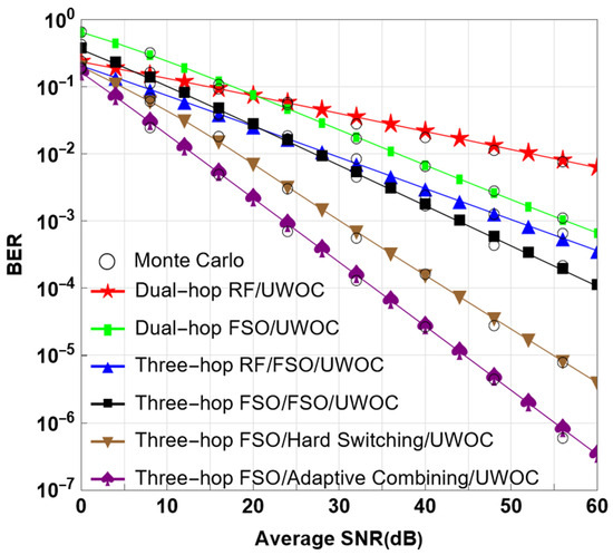
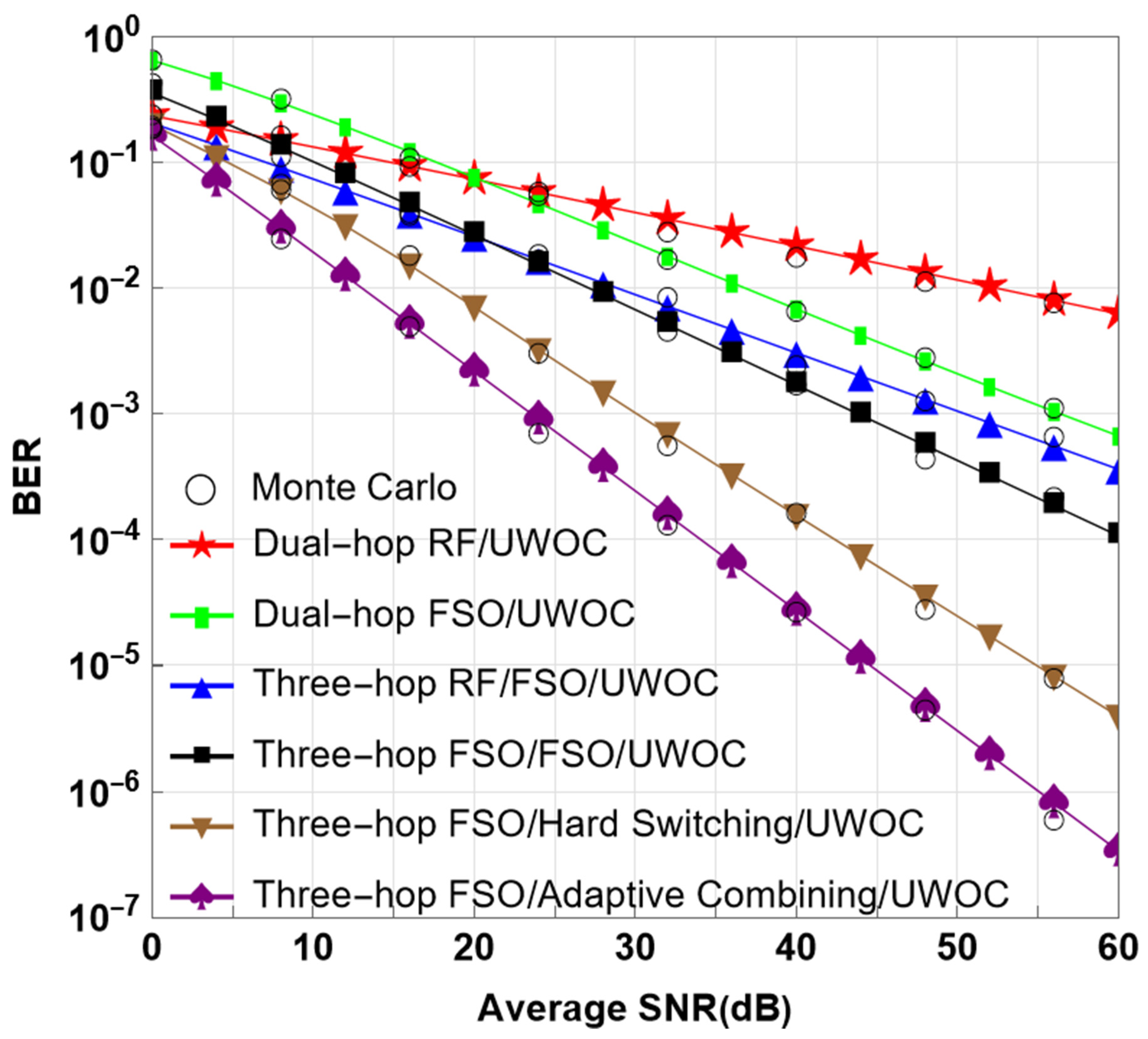
For Figure 3, the horizontal-axis variable ${\rho }_{\mathrm{d}\mathrm{B}}$ denotes a normalized reference post-detection average electrical SNR. For the i-th architecture, the effective average SNR used in the BER calculation is ${\stackrel{-}{\gamma }}_{i,\mathrm{d}\mathrm{B}}=a_i{\rho }_{\mathrm{d}\mathrm{B}}+b_i$, where $a_i$ and $b_i$ are route-dependent mapping parameters specified in the simulation settings. The resulting average SNR is applied synchronously to all active links of the corresponding dual-hop or three-hop architecture. Therefore, owing to the different link types and numbers of hops, the actual link SNRs are not necessarily identical among the compared schemes.

Figure 3. BER performance comparison of the three-hop heterogeneous space–air–sea communication system under different transmission schemes.

The scheme-specific coefficient pairs are listed in Table 5. Here, $a_i$ is a dimensionless slope, and $b_i$ is an additive offset expressed in dB.

Table 5. Scheme-specific SNR-mapping coefficients for Figure 3.

Transmission Scheme	${\mathit{a}}_{\mathit{i}}$	${\mathit{b}}_{\mathit{i}}\left(\mathit{d}\mathit{B}\right)$
Dual-hop RF/UWOC	0.32997268	4.85751972
Dual-hop FSO/UWOC	0.75081562	−0.03105999
Three-hop RF/FSO/UWOC	0.63170002	10.28494865
Three-hop FSO/FSO/UWOC	0.83832972	8.46120704
Three-hop FSO/Hard Switching/UWOC	1.10220421	9.33548339
Three-hop FSO/Adaptive Combining/UWOC	1.26950000	11.92923621

For the subsequent numerical results, the proposed three-hop FSO/adaptive FSO–RF/UWOC architecture and the common SNR mapping ${\stackrel{-}{\gamma }}_{\mathrm{e}\mathrm{f}\mathrm{f},\mathrm{d}\mathrm{B}}=1.2695{\rho }_{\mathrm{d}\mathrm{B}}+11.92923621$ are retained. The $10 \mathrm{d}\mathrm{B}$ value listed for the RF branch in Table 2 denotes the nominal baseline value of the reference parameter configuration. In the subsequent numerical evaluations, however, ${\overline{\gamma }}_2^{\mathrm{R}\mathrm{F}}$ is not fixed at $10 \mathrm{d}\mathrm{B}$ but is varied synchronously with the reference average SNR according to the corresponding SNR mapping. Accordingly, the nominal average SNRs of the first-hop FSO link, the second-hop FSO link, the RF branch when activated, and the UWOC link are varied synchronously. For the subsequent numerical evaluations, only one group of parameters is varied at a time: the 16-ary modulation format; the pointing displacement and jitter parameters; the WGG turbulence parameters and detection exponent $R_3$; and $d_{\mathrm{B}\mathrm{U}}=10,\hspace{0.33em}30,\hspace{0.33em}50,$ and $70 \mathrm{m}$ together with $R_3$, where ${\rho }_{\mathrm{d}\mathrm{B}}$ represents the reference average SNR at $d_0=10 \mathrm{m}$, and ${\overline{\gamma }}_{\mathrm{U}\mathrm{W}\mathrm{O}\mathrm{C}}\left(d_{\mathrm{B}\mathrm{U}}\right)={\overline{\gamma }}_{\mathrm{r}\mathrm{e}\mathrm{f}}{\left({\displaystyle \frac{d_{\mathrm{B}\mathrm{U}}}{10 \mathrm{m}}}\right)}^{-2}$; and the shadowed-Rician parameters $\left(m,\hspace{0.33em}2b_0,\hspace{0.33em}\mathsf{\Omega }\right)$. All other parameters are kept fixed within each numerical evaluation.

For normalized resource accounting, the constellation symbols are normalized to unit average energy, $E_{s,\mathrm{n}\mathrm{o}\mathrm{r}\mathrm{m}}=1$, while the end-to-end transmit-energy budget is separately normalized to $E_{\mathrm{t}\mathrm{o}\mathrm{t}\mathrm{a}\mathrm{l},\mathrm{n}\mathrm{o}\mathrm{r}\mathrm{m}}=1$. All schemes also use $M=16$, $B_{\mathrm{n}\mathrm{o}\mathrm{r}\mathrm{m}}=1$, and $T_{\mathrm{s}\mathrm{l}\mathrm{o}\mathrm{t},\mathrm{n}\mathrm{o}\mathrm{r}\mathrm{m}}=1$. The normalized total energy is uniformly allocated among the active hops, giving $E_{\mathrm{h}\mathrm{o}\mathrm{p},\mathrm{n}\mathrm{o}\mathrm{r}\mathrm{m}}=1/2$ for dual-hop schemes and $E_{\mathrm{h}\mathrm{o}\mathrm{p},\mathrm{n}\mathrm{o}\mathrm{r}\mathrm{m}}=1/3$ for three-hop schemes. A common three-slot comparison frame is adopted, corresponding to an end-to-end spectral efficiency of ${\eta }_{\mathrm{e}2\mathrm{e}}={\mathrm{l}\mathrm{o}\mathrm{g}}_2\left(16\right)/3=4/3$ bit/s/Hz. The RF branch is activated when ${\gamma }_2^{\mathrm{F}\mathrm{S}\mathrm{O}}<{\gamma }_T$, where ${\gamma }_{T,\mathrm{d}\mathrm{B}}=5 \mathrm{d}\mathrm{B}$, equivalently ${\gamma }_T={10}^{{\gamma }_{T,\mathrm{d}\mathrm{B}}/10}$. Thus, $P_{\mathrm{a}\mathrm{c}\mathrm{t}}=\mathrm{P}\mathrm{r}({\gamma }_2^{\mathrm{F}\mathrm{S}\mathrm{O}}<{\gamma }_T)$, and with $E_{\mathrm{R}\mathrm{F},\mathrm{o}\mathrm{n},\mathrm{n}\mathrm{o}\mathrm{r}\mathrm{m}}=1$, the normalized average RF energy is ${\stackrel{-}{E}}_{\mathrm{R}\mathrm{F},\mathrm{n}\mathrm{o}\mathrm{r}\mathrm{m}}=P_{\mathrm{a}\mathrm{c}\mathrm{t}}$. In Figure 3, $P_{\mathrm{a}\mathrm{c}\mathrm{t}}$ decreases approximately from $0.4572$ at $0$ dB to $1.03\times {10}^{-5}$ at $60$ dB for hard switching, whereas it decreases from approximately $0.3268$ to $9.54\times {10}^{-7}$ for adaptive combining. The different activation probabilities of the hard-switching and adaptive-combining schemes arise from their scheme-specific second-hop FSO-SNR mappings in Figure 3. Accordingly, these normalized assumptions provide a common resource-accounting basis for all considered schemes in terms of energy, bandwidth, transmission time, and end-to-end spectral efficiency.

Figure 3 presents the BER performance comparison of the three-hop heterogeneous space–air–sea communication system under different transmission schemes as the average SNR varies. It can be observed that the BERs of all transmission schemes decrease as the average SNR increases, indicating that improving the average link SNR can effectively improve the BER performance of the system. Meanwhile, the Monte Carlo simulation results are in good agreement with the theoretical analytical curves, which verifies the correctness of the derived analytical BER expressions.

From the performance comparison of different schemes, it can be seen that the dual-hop RF/UWOC scheme exhibits the worst BER performance. This indicates that when only the RF link is used for the space-to-sea-surface transmission segment, the end-to-end BER remains relatively high. In contrast, the dual-hop FSO/UWOC scheme performs better in the medium- and high-SNR regions. This is because, under favorable channel conditions, the FSO link can fully exploit its advantages of a high data rate and low-error transmission. However, under low-SNR conditions, the received signal power is relatively weak, and the BER performance of the FSO link is more significantly affected by atmospheric turbulence, path loss, and pointing errors.

Furthermore, compared with the three-hop scheme, the FSO/Hard Switching/UWOC scheme outperforms the fixed three-hop transmission structure, indicating that the link-switching mechanism can improve the reliability of the HAP-to-buoy link. The proposed three-hop FSO/adaptive combining/UWOC scheme achieves the lowest BER over the entire SNR range, and its advantage becomes more pronounced in the medium- and high-SNR regions. This is because the proposed scheme can not only use the RF link as compensation under low-SNR conditions or when the FSO link is impaired, but also fully exploit the low-error transmission advantage of the FSO link under high-SNR conditions. Therefore, the reliability of the HAP-to-sea-surface buoy link is enhanced, and the end-to-end BER performance is further improved. These results demonstrate that the proposed adaptive combining transmission mechanism can fully exploit the complementary advantages of FSO and RF links, thereby effectively improving the end-to-end transmission reliability of the three-hop heterogeneous space–air–sea communication system.

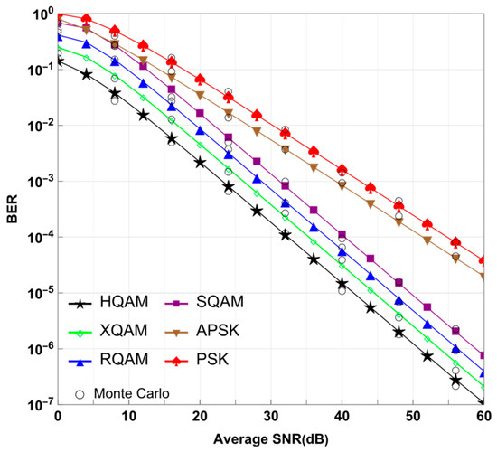
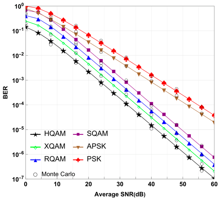
Across the subsequent numerical results, the Monte Carlo markers closely follow the analytical curves. Where asymptotic curves are shown, they approach the analytical results in the high-SNR region. Figure 4 compares the BER performance of the considered 16-ary modulation schemes.

Figure 4. BER performance comparison of the three-hop heterogeneous space–air–sea communication system under different 16-ary modulation schemes.

Phase-shift keying (PSK) and amplitude phase-shift keying (APSK) exhibit the highest BERs, while square quadrature amplitude modulation (SQAM) and rectangular quadrature amplitude modulation (RQAM) provide intermediate performance. Cross quadrature amplitude modulation (XQAM) outperforms SQAM and RQAM, whereas HQAM achieves the lowest BER over the considered SNR range. This performance ordering is mainly attributed to differences in constellation geometry and symbol separation, which affect the sensitivity of the decision regions to noise and channel fading.

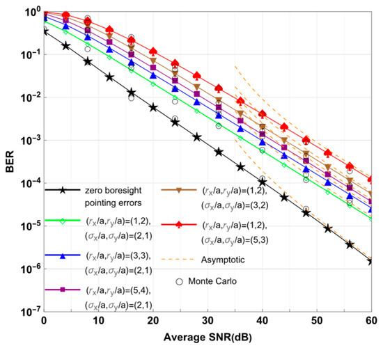
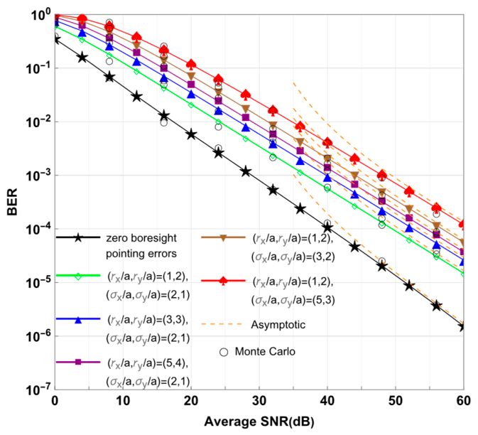
Figure 5 shows the BER performance under different boresight pointing-error parameters.

Figure 5. BER performance comparison of the three-hop heterogeneous space–air–sea communication system under different boresight pointing error parameters.

Figure 5 shows close agreement between the analytical and Monte Carlo results, while the asymptotic curves approach the analytical curves at a high SNR. The zero-boresight case yields the lowest BER. Larger boresight displacement and pointing jitter increase the BER because stronger misalignment reduces the collected optical power.

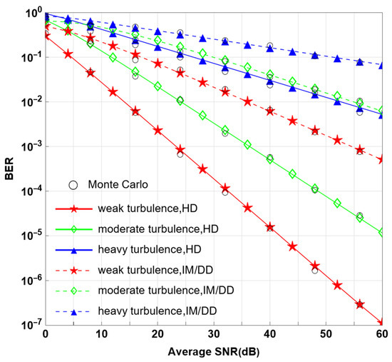
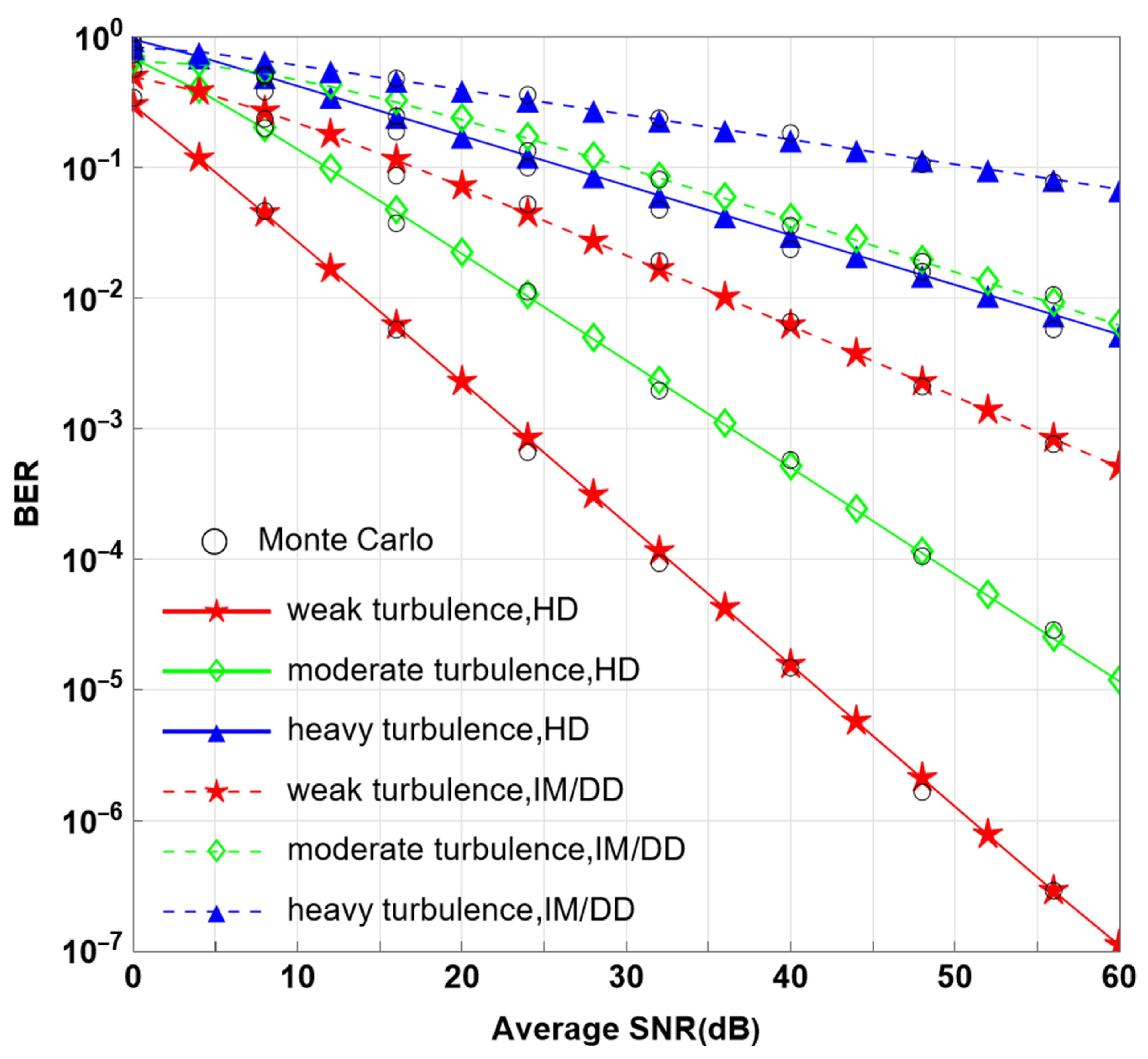
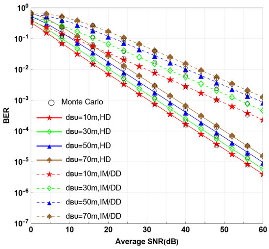
Figure 6 illustrates the effects of underwater turbulence and detection techniques.

Figure 6. BER performance comparison of the three-hop heterogeneous space–air–sea communication system under different underwater turbulence conditions and detection techniques.

For both HD and IM/DD, the BER decreases as the average SNR increases. Stronger underwater turbulence shifts the BER curves upward because larger irradiance fluctuations degrade the buoy-to-AUV optical link. Under the same turbulence condition, HD consistently achieves a lower BER than IM/DD, particularly in the medium- and high-SNR regions.

Figure 7 illustrates the effects of underwater transmission distance and detection technique.

Figure 7. BER performance comparison of the three-hop heterogeneous space–air–sea communication system under different underwater transmission distances and detection techniques.

The BER decreases as the average SNR increases in all cases. Increasing the transmission distance from 10 m to 70 m shifts the BER curves upward because greater underwater attenuation reduces the received optical power. At the same distance, HD consistently outperforms IM/DD, particularly in the medium- and high-SNR regions.

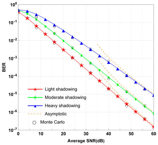
Figure 8 illustrates the effects of different shadowed-Rician fading conditions.

Figure 8. BER performance comparison of the three-hop heterogeneous space–air–sea communication system under different shadowed fading conditions.

The analytical and Monte Carlo results agree closely, while the asymptotic curves approach the analytical curves in the high-SNR region. The light-shadowing case achieves the lowest BER, whereas moderate and heavy shadowing shift the BER curves upward. This degradation occurs because more severe shadowing degrades the reliability of the HAP-to-buoy RF backup branch.

5. Conclusions

In this paper, a three-hop heterogeneous space–air–sea communication system jointly considering nonzero-boresight pointing errors and an adaptive combining scheme for mixed FSO/RF transmission was proposed for complex space–air–sea cross-domain communication scenarios. The system adopts the DF relaying protocol and consists of a satellite, a HAP, a sea-surface buoy, and an AUV. Specifically, the satellite-to-HAP link employs FSO transmission, the HAP-to-sea-surface buoy link adopts an adaptive combining scheme for mixed FSO/RF transmission, and the sea-surface buoy-to-AUV link employs UWOC transmission. To more accurately characterize the impact of alignment mismatch in practical optical links, a nonzero-boresight pointing error model was introduced into the two FSO links and the UWOC link. Moreover, the fading characteristics of different links were modeled by the Málaga-$ℳ$ distribution, the shadowed-Rician distribution, and the WGG distribution, respectively. On this basis, an analytical expression for the end-to-end average BER of the system was derived, and the theoretical analysis was validated through Monte Carlo simulations.

The simulation results show that the average BER of the system gradually decreases as the average SNR increases, and the theoretical curves agree well with the Monte Carlo simulation results, which verifies the validity of the derived analytical BER expressions. Compared with conventional dual-hop schemes and hard-switching schemes, the proposed adaptive combining scheme for mixed FSO/RF transmission can flexibly select the transmission mode according to the link state and introduce the RF branch to enhance link stability when the FSO link is impaired, thereby improving the end-to-end transmission reliability of the three-hop heterogeneous space–air–sea communication system. The comparison of different modulation schemes indicates that, under the same 16-ary modulation order, HQAM achieves the best BER performance, demonstrating that optimizing the modulation constellation structure can effectively reduce the system BER. In addition, nonzero-boresight pointing errors significantly degrade system performance, and the BER further increases with the increase in boresight displacement and random jitter. Stronger underwater turbulence, longer underwater transmission distance, and more severe shadowed fading of the RF link all lead to degraded BER performance. Meanwhile, under the same underwater turbulence and transmission distance conditions, HD achieves better BER performance than IM/DD. In summary, the proposed three-hop heterogeneous space–air–sea communication system can improve end-to-end transmission reliability through the integration of FSO, RF, and UWOC links. The results of this work can provide theoretical guidance for link design and parameter optimization of cross-domain heterogeneous communication systems in complex space–air–sea environments.

The present analysis assumes independent block fading, perfect CSI, ideal synchronization, a fixed switching threshold, and a quasi-static buoy-to-AUV UWOC link, while practical switching delay, channel correlation, AUV mobility, detailed hardware-level and system-level energy consumption, and hardware impairments are not explicitly modeled. Future work will investigate imperfect CSI, time-varying correlated channels, mobility-aware transmission, energy-aware threshold optimization, practical switching and processing delays, and experimental validation. In addition, a hybrid UAC/UWOC underwater link with environment-aware switching will be explored to combine the high data rate of UWOC with the wider coverage and stronger robustness of acoustic communication.

References

- Sharif, S.; Zeadally, S.; Ejaz, W. Space-aerial-ground-sea integrated networks: Resource optimization and challenges in 6G. J. Netw. Comput. Appl. 2023, 215, 103647. [Google Scholar] [CrossRef] [Scilit]
- Zhao, H.; Ji, F.; Wang, Y.; Yao, K.; Chen, F. Space-Air-Ground-Sea Integrated Network with Federated Learning. Remote Sens. 2024, 16, 1640. [Google Scholar] [CrossRef] [Scilit]
- Jung, S.; Jeong, S.; Kang, J.; Kang, J. Marine IoT Systems With Space-Air-Sea Integrated Networks: Hybrid LEO and UAV Edge Computing. IEEE Internet Things J. 2023, 10, 20498–20510. [Google Scholar] [CrossRef] [Scilit]
- Jahid, A.; Alsharif, M.H.; Hall, T.J. A Contemporary Survey on Free Space Optical Communication: Potentials, Technical Challenges, Recent Advances and Research Direction. J. Netw. Comput. Appl. 2022, 200, 103311. [Google Scholar] [CrossRef] [Scilit]
- Arum, S.C.; Grace, D.; Mitchell, P.D. A Review of Wireless Communication Using High-Altitude Platforms for Extended Coverage and Capacity. Comput. Commun. 2020, 157, 232–256. [Google Scholar] [CrossRef] [Scilit]
- Yahia, O.B.; Erdogan, E.; Kurt, G.K.; Altunbas, I.; Yanikomeroglu, H. HAPS Selection for Hybrid RF/FSO Satellite Networks. IEEE Trans. Aerosp. Electron. Syst. 2022, 58, 2855–2867. [Google Scholar] [CrossRef] [Scilit]
- Swaminathan, R.; Sharma, S.; Vishwakarma, N.; Madhukumar, A.S. HAPS-Based Relaying for Integrated Space-Air-Ground Networks with Hybrid FSO/RF Communication: A Performance Analysis. IEEE Trans. Aerosp. Electron. Syst. 2021, 57, 1581–1599. [Google Scholar] [CrossRef] [Scilit]
- Mohsan, S.A.H.; Khan, M.A.; Amjad, H. Hybrid FSO/RF Networks: A Review of Practical Constraints, Applications and Challenges. Opt. Switch. Netw. 2023, 47, 100697. [Google Scholar] [CrossRef] [Scilit]
- Junejo, N.U.R.; Habaebi, M.H.; Islam, M.R. A Survey on Physical Layer Techniques and Challenges in Underwater Acoustic Communication. J. Mar. Sci. Eng. 2023, 11, 885. [Google Scholar] [CrossRef] [Scilit]
- Saeed, N.; Celik, A.; Al-Naffouri, T.Y.; Alouini, M.-S. Underwater Optical Wireless Communications, Networking, and Localization: A Survey. Ad. Hoc Netw. 2019, 94, 101935. [Google Scholar] [CrossRef] [Scilit]
- Li, G.; Wang, J.; Dai, J.; Zhao, T.; Chen, D.; Chen, C. Adaptive Path Planning for Autonomous Underwater Vehicle (AUV) Based on Spatio-Temporal Graph Neural Networks and Conditional Normalizing Flow Probabilistic Reconstruction. Algorithms 2026, 19, 147. [Google Scholar] [CrossRef] [Scilit]
- Palitharathna, K.W.S.; Suraweera, H.A.; Godaliyadda, R.I.; Herath, V.R.; Thompson, J.S. Multi-AUV Placement for Coverage Maximization in Underwater Optical Wireless Sensor Networks. In Proceedings of the 2020 Global Oceans 2020: Singapore–U.S. Gulf Coast, Biloxi, MS, USA, 5–30 October 2020; pp. 1–8. [Google Scholar]
- Gamal, C.; Elsayed, M.; Samir, A.; Tageldien, H.A.; Chatzinotas, S.; Fouda, M.M.; ElHalawany, B.M. Reliability of Spectrum-Efficient Mixed Satellite-Underwater Systems. IEEE Open J. Commun. Soc. 2022, 3, 2237–2244. [Google Scholar] [CrossRef] [Scilit]
- Teng, T.; He, A. Performance of Satellite UWOC Network with Generalized Boresight Error and AWGGN. Radioengineering 2023, 32, 616–624. [Google Scholar] [CrossRef] [Scilit]
- Zhou, S.; Ding, D.; Wang, J.; Yang, D.; Yuan, S. Performance Analysis of Hybrid RF-UWOC Dual-Hop Link for Satellite-Underwater Communication. Proc. SPIE 2024, 13153, 131530V. [Google Scholar] [CrossRef] [Scilit]
- Rahman, Z.; Zafaruddin, S.M.; Chaubey, V.K. Direct Air-to-Underwater Optical Wireless Communication: Statistical Characterization and Outage Performance. IEEE Trans. Veh. Technol. 2023, 72, 2655–2660. [Google Scholar] [CrossRef] [Scilit]
- Li, S.; Yang, L.; da Costa, D.B.; Yu, S. Performance Analysis of UAV-Based Mixed RF-UWOC Transmission Systems. IEEE Trans. Commun. 2021, 69, 5559–5572. [Google Scholar] [CrossRef] [Scilit]
- Devaja, T.; Petkovic, M.; Beko, M.; Vukobratovic, D. Performance Analysis of UAV-Assisted RF-UOWC Systems. In Proceedings of the 2024 7th International Balkan Conference on Communications and Networking (BalkanCom), Ljubljana, Slovenia, 3–6 June 2024; pp. 280–284. [Google Scholar]
- Nallagonda, V.R.; Maturi, R.R.; Manchikalapudi, S.S.R.; Dantuluri, B. Performance Analysis of High-Altitude Platform-Underwater Wireless Optical Communication Systems with Decode-and-Forward Relaying. Opt. Eng. 2026, 65, 026101. [Google Scholar] [CrossRef] [Scilit]
- Sarma, P.; Deka, R.; Anees, S. Performance Analysis of DF-Based Mixed Triple-Hop RF-FSO-UWOC Cooperative System. In Proceedings of the 2020 IEEE 92nd Vehicular Technology Conference (VTC2020-Fall), Victoria, BC, Canada, 18 November–16 December 2020; pp. 1–5. [Google Scholar]
- Yadav, S.; Aggarwal, M.; Ahuja, S.; Vats, A.; Sabherwal, P. Performance Analysis of UAV Assisted Triple-Hop Mixed FSO/RF/UWOC System with Altitude Optimization. J. Opt. Commun. 2024, 45, s1851–s1861. [Google Scholar] [CrossRef] [Scilit]
- Bankey, V.; Sharma, S.; Swaminathan, R.; Madhukumar, A.S. Physical Layer Security of HAPS-Based Space-Air-Ground-Integrated Network With Hybrid FSO/RF Communication. IEEE Trans. Aerosp. Electron. Syst. 2023, 59, 4680–4688. [Google Scholar] [CrossRef] [Scilit]
- Payal, N.; Gurjar, D.S. Hybrid FSO/RF and UWOC System for Enabling Terrestrial-Underwater Communication: Performance Analysis. Phys. Commun. 2025, 68, 102540. [Google Scholar] [CrossRef] [Scilit]
- Alhalabi, M.; Sonmezocak, T.; El-Nahal, F. Design and Performance Analysis of a Directly Modulated Direct Current-Biased Optical Orthogonal Frequency-Division Multiplexing Visible-Light Optical Wireless Link Under Atmospheric Turbulence. Appl. Sci. 2026, 16, 6324. [Google Scholar] [CrossRef] [Scilit]
- Alhalabi, M.; Taşpınar, N.; Wadi, M.; Salemdeeb, M. Performance Analysis of a Low-Cost Directly Modulated OFDM-Based Optical Wireless Communication Systems. Wirel. Pers. Commun. 2026, 146, 1415–1441. [Google Scholar] [CrossRef] [Scilit]
- Alhalabi, M. Performance Analysis of a 16-QAM Directly Modulated OFDM Visible Optical Wireless Link Without External Modulators. J. Opt. Photonics Res. 2026; Online First. [CrossRef] [Scilit]
- Liu, X.; Lin, M.; Zhu, W.-P.; Wang, J.-Y.; Upadhyay, P.K. Outage Performance for Mixed FSO-RF Transmission in Satellite-Aerial-Terrestrial Networks. IEEE Photonics Technol. Lett. 2020, 32, 1349–1352. [Google Scholar] [CrossRef] [Scilit]
- Hao, W.; Wang, P.; Pang, W.; Zhou, B.; Zhang, L. Performance Analysis of an AUV-Aided NOMA-Based Vertical UWOC System With a Cascaded WGG Turbulence Model. J. Opt. Soc. Am. A 2024, 41, 2112–2124. [Google Scholar] [CrossRef] [Scilit] [PubMed]
- Yang, F.; Cheng, J.; Tsiftsis, T.A. Free-Space Optical Communication With Nonzero Boresight Pointing Errors. IEEE Trans. Commun. 2014, 62, 713–725. [Google Scholar] [CrossRef] [Scilit]
- Ansari, I.S.; Yilmaz, F.; Alouini, M.-S. Performance Analysis of Free-Space Optical Links Over Málaga () Turbulence Channels With Pointing Errors. IEEE Trans. Wirel. Commun. 2016, 15, 91–102. [Google Scholar] [CrossRef] [Scilit]
- Alshaer, N.; Ismail, T.; Nasr, M.E. Generic Evaluation of FSO System Over Málaga Turbulence Channel With MPPM and Nonzero-Boresight Pointing Errors. IET Commun. 2020, 14, 1534–1542. [Google Scholar] [CrossRef] [Scilit]
- Abdi, A.; Lau, W.C.; Alouini, M.-S.; Kaveh, M. A New Simple Model for Land Mobile Satellite Channels: First- and Second-Order Statistics. IEEE Trans. Wirel. Commun. 2003, 2, 519–528. [Google Scholar] [CrossRef] [Scilit]
- Zhou, B.; Wang, P.; Cao, T.; Li, G.; Li, S.; Yang, P. Performance Analysis of AUV-Carried RISs-Aided Multihop UWOC Convergent With RF MRC Systems Over WGG Oceanic Turbulence. Veh. Commun. 2024, 45, 100722. [Google Scholar] [CrossRef] [Scilit]
- Qiu, H.; Huang, Z.; Xu, J.; Zhai, W.; Gao, Y.; Ji, Y. Unified Statistical Thermocline Channel Model for Underwater Wireless Optical Communication. Opt. Lett. 2023, 48, 636–639. [Google Scholar] [CrossRef] [Scilit] [PubMed]
- Morgado, E.; Mora-Jiménez, I.; Vinagre, J.J.; Ramos, J.; Caamaño, A.J. End-to-End Average BER in Multihop Wireless Networks over Fading Channels. IEEE Trans. Wirel. Commun. 2010, 9, 2478–2487. [Google Scholar] [CrossRef] [Scilit]
- Bilim, M. Different QAM Schemes Analyses for ARS Fading Channels. Trans. Emerg. Telecommun. Technol. 2021, 32, e4119. [Google Scholar] [CrossRef] [Scilit]
- Yilmaz, F.; Alouini, M.-S. A Novel Unified Expression for the Capacity and Bit Error Probability of Wireless Communication Systems over Generalized Fading Channels. IEEE Trans. Commun. 2012, 60, 1862–1876. [Google Scholar] [CrossRef] [Scilit]
- Trott, M. The Wolfram Functions Site. Available online: http://functions.wolfram.com (accessed on 1 July 2026).
- Vishwakarma, N.; Sharma, S.; Madhukumar, A.S. On the Maximal-Ratio Combining of FSO and RF Links Over Generalized Fading Channels. Optik 2022, 266, 169564. [Google Scholar]
Disclaimer/Publisher’s Note: The statements, opinions and data contained in all publications are solely those of the individual author(s) and contributor(s) and not of MDPI and/or the editor(s). MDPI and/or the editor(s) disclaim responsibility for any injury to people or property resulting from any ideas, methods, instructions or products referred to in the content. |
© 2026 by the authors. Licensee MDPI, Basel, Switzerland. This article is an open access article distributed under the terms and conditions of the Creative Commons Attribution (CC BY) license.