A Physics-Guided Dehazing Method Based on Polarization Imaging

Abstract

Haze conditions degrade image quality via atmospheric scattering and absorption, posing challenges for optical imaging applications. In recent years, deep learning has emerged as an effective method for dehazing images. However, data-driven deep learning dehazing methods typically require large amounts of labeled training data and offer limited interpretability. In this paper, we propose a physics-guided dehazing method based on polarization imaging. By integrating polarization imaging with the physical model, the proposed method enables neural network training using only a set of hazy images captured at different polarization angles, thereby reducing the reliance on labeled training data. Experimental results show that the proposed method significantly outperforms commonly used deep learning dehazing methods in terms of contrast and mean gradient, while exhibiting strong generalization and physical interpretability. By integrating physical model and polarization imaging into deep learning, this method overcomes the limitations of traditional deep learning dehazing methods and paves the way for optical imaging in haze conditions.

1. Introduction

Hazy conditions pose severe challenges to fields such as transportation, aviation, and environmental monitoring. In transportation, hazy conditions lead to a sharp decline in visibility, significantly increasing the risk of traffic accidents and compromising the safety and efficiency of public transport [1]. In environmental monitoring, hazy conditions obscure visibility, making it difficult to measure key indicators such as air quality and visibility, thereby affecting the accuracy and timeliness of environmental data [2,3]. Therefore, research on dehazing methods is of great significance for improving the quality of images under hazy conditions.

Existing dehazing methods are mainly divided into physical model-based and deep learning-based. Physical model-based methods exploit physical priors and assumptions to estimate the key parameters required for dehazing, such as the dark channel prior (DCP) [4], boundary constraint and contextual regularization (BCCR) [5], and the color attenuation prior (CAP) [6]. These methods are grounded in the atmospheric scattering model and rely on intensity information from a single hazy image, together with statistical regularities or physical priors, to estimate key model parameters, most notably the transmission $t\left(x\right)$ and airlight $A$, and then recover a dehazed image via model inversion. However, real-world atmospheric scattering and absorption are often more complex than model assumptions. Estimating $t\left(x\right)$ and $A$ using only intensity makes it difficult to fully characterize the true degradation process. This issue is pronounced in complex outdoor conditions, these methods struggle to recover fine details [7,8]. To improve the accuracy of parameter estimation beyond relying solely on intensity, one can incorporate polarimetric information that reflects the medium’s scattering characteristics. The polarimetric properties of light reflected from a target are closely related to its surface roughness, geometry, material properties, and structural characteristics. Compared with conventional intensity imaging, polarimetric imaging provides stronger target enhancement in complex backgrounds and under low-visibility conditions, offering a clear advantage [9].

Polarization-based dehazing leverages the polarization characteristics of $A$. For a given scene, four polarimetric images are captured at different rotating polarizer angles (e.g., 0°, 45°, 90°, and 135°). From the Stokes vector, two parameters closely tied to the properties of scattered light are computed: the degree of linear polarization P and the angle of polarization θ. These provide physical constraints for estimating $t\left(x\right)$ and $A$. Combined with the atmospheric scattering model, these constraints yield the dehazed image. This method preserves fine object details and has significant practical value for image dehazing. Building on this, Wu et al. incorporated the Polarization Block-Matching and 3D Filtering denoising technique, effectively suppressing noise and improving dehazing performance under dense fog conditions [10]. Liang et al. introduced low-pass filtering to suppress noise in polarization images under dense fog, improving the accuracy of $t\left(x\right)$ estimation and thereby enhancing dehazing performance [11]. Despite providing physical constraints for estimating $t\left(x\right)$ and $A$, polarization-based dehazing still faces limitations in practical applications. In outdoor conditions, climate and illumination vary significantly over time. Changes in solar elevation and azimuth and cloud cover alter the spatial distribution and polarization of airlight, introducing errors in estimating P and θ and reducing the accuracy of $t\left(x\right)$ and $A$ estimation [12].

Deep learning is a powerful method for modeling complex relationships and has steadily matured in image dehazing due to its strong performance [13,14]. Deep learning methods typically rely on large, high-quality paired datasets to train end-to-end convolutional neural networks, such as DehazeNet [15], lightweight models like AOD [16], or architectures based on DehazeFormer [17], to learn the mapping from hazy images to clear images. Recent studies have further extended learning-based image restoration to challenging conditions, including underground and nighttime dehazing, remote-sensing image dehazing, and depth completion for scene-structure recovery [18,19,20,21]. Compared with physical model-based dehazing methods, deep learning-based methods can extract multi-scale features and demonstrate greater robustness and dehazing performance in complex haze conditions [22,23,24]. However, this method is highly dependent on high-quality paired training data; in complex haze conditions, data acquisition is costly and has limited coverage, leading to insufficient cross-domain generalization of the model [25,26]. Moreover, most current deep learning dehazing methods are end-to-end and data-driven, with limited physical interpretability. To address these issues, researchers have explored an unsupervised mechanism combined with physical priors. For example, the polarization-based unsupervised dehazing network [27], which incorporates polarimetric measurements, has achieved certain improvements in generalization. However, in outdoor conditions, the strongly time-varying illumination and weather, and the scarcity of high-quality paired data pose significant challenges to the generalization and interpretability of existing deep learning dehazing methods.

Here, we propose a physics-guided dehazing method based on polarization imaging. The main contributions of this work are summarized as follows. First, the network is optimized separately for each scene from random initialization using only four polarimetric images of the same scene, without requiring paired data or an external training dataset. Second, a three-component loss function is designed by combining the physical-consistency reconstruction loss, TV loss, and DCP loss to maintain physical consistency, suppress noise and over-enhancement, and reduce residual haze. Experimental results on synthetic and real polarimetric data show that the proposed method achieves favorable performance in both qualitative and quantitative evaluations.

2. Methodology

2.1. Atmospheric Scattering Model

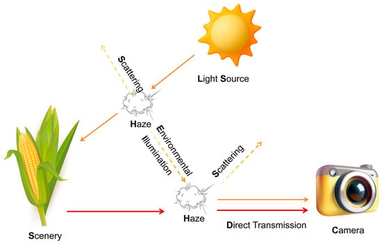
Figure 1 illustrates the atmospheric scattering model. In hazy conditions, suspended aerosol particles scatter and absorb incident light, attenuating the direct transmission and redirecting photons from their original paths before they reach the imaging system. During propagation, a portion of the light is scattered by aerosols into the camera’s line of sight, producing an approximately spatially uniform airlight. The remainder of the light illuminates scene surfaces, is reflected, and, while traversing the hazy medium, undergoes attenuation before finally reaching the image plane as direct transmission. At the image plane, these two components sum to form the observed pixel intensity. This image formation process can be expressed as follows [28]:

$$I\left(x\right)=J\left(x\right)t\left(x\right)+A\left[1-t\left(x\right)\right],$$

(1)

where $I\left(x\right)$ denotes the captured image intensity at pixel location $x$, $J\left(x\right)$ denotes the target reflected light, $A$ denotes the spatially uniform airlight, and $t\left(x\right)$ denotes the transmission characterizing attenuation and is expressed as

$$t\left(x\right)=exp\left(-\beta d\left(x\right)\right),$$

(2)

where $\beta$ and $d\left(x\right)$ denote the scattering coefficient and scene depth, respectively. In haze, $t\left(x\right)$ decays exponentially with depth, degrading contrast and fine details. $\beta$ depends on aerosol size, concentration, and wavelength, and can vary spatially under non-uniform haze.

Figure 1. Schematic illustration of the atmospheric scattering model.

Equation (1) shows that the key to image dehazing lies in accurately estimating $t\left(x\right)$ and $A$, which enables effective recovery of the dehazed image $J\left(x\right)$. In complex real-world hazy conditions, spatial non-uniformity in $t\left(x\right)$ and $A$ renders the inversion ill-posed, leading to inaccurate parameter estimates and heightened noise sensitivity [29].

2.2. Polarized Image Information

In the atmospheric scattering model, conventional imaging systems typically rely on image intensity to estimate $A$ and $t\left(x\right)$. However, in real-world hazy conditions, $A$ and $J\left(x\right)$ are heavily intermixed spatially, and intensity alone cannot reliably separate them, which degrades dehazing performance. Polarimetric imaging captures both intensity and polarization, providing additional information to distinguish $A$ from $J\left(x\right)$, and enabling them to be estimated more accurately, thus improving dehazing performance. According to scattering theory, Mie scattering of incident light by atmospheric aerosol particles imparts distinct polarization properties to the scattered light. To describe the polarization state of the incident light using the Stokes vector, images are captured with rotating polarizer angles of 0°, 45°, 90°, and 135° ($I_0$, $I_{45}$, $I_{90}$, $I_{135}$). The Stokes parameters $S_0$, $S_1$ and $S_2$ can be expressed as follows [30]:

$$\left\{\begin{array}{l}{S}_0=I_0+I_{90}\\ S_1=I_0-I_{90}\\ S_2=I_{45}-I_{135}\end{array}\right.,$$

(3)

where $S_0$ denotes the total intensity, that is, $I\left(x\right)$ in the atmospheric scattering model, $S_1$ denotes the intensity difference between the 0° and 90° polarization orientations, and $S_2$ denotes the intensity difference between 45° and 135°. Based on the Stokes parameters, $P$ and $\theta$ can be obtained, which are expressed as follows:

$$P={\displaystyle \frac{\sqrt{S_1^2+S_2^2}}{S_0}},$$

(4)

$$\theta ={\displaystyle \frac{1}{2}}arctan\left({\displaystyle \frac{S_2}{S_1}}\right).$$

(5)

From Equations (4) and (5), it can be seen that $P$ is related to $S_0$, whereas $\theta$ is independent of $S_0$. In hazy conditions, the polarization information of $J\left(x\right)$ is very weak, primarily reflected in $S_0$, with little influence on $S_1$ and $S_2$. According to Equation (5), the polarization angle of each pixel in the image is computed, the polarization angle with the highest occurrence probability is selected as the airlight polarization angle ${\theta }_A$, the degree of polarization from the pixels that satisfy this angle is then computed, and the maximum value is taken as the airlight degree of polarization $P_A$. This estimation assumes that a single dominant airlight polarization angle exists within the scene. In scenes with complex scattering conditions, the polarization-angle distribution may have multiple peaks, and using a single value of ${\theta }_A$ for the entire scene may introduce errors in the estimation of airlight and transmission. Using the estimated ${\theta }_A$ and $P_A$, the polarized component of the airlight can be expressed as follows:

$$A_p={\displaystyle \frac{I_0-S_0(1-P)/2}{{cos}^2{\theta }_A}}={\displaystyle \frac{I_{90}-S_0(1-P)/2}{{sin}^2{\theta }_A}},$$

(6)

and according to $A=A_p/P_A$, together with Equation (6), $A$ can be obtained.

The expression for the infinity airlight intensity estimated using the Stokes parameters is as follows:

$$A_{\infty }(x,y)={\displaystyle \frac{2I_0}{1+P_A{cos}^2{\theta }_A}},$$

(7)

and given A and $t(x)=A/A_{\infty }$, together with Equation (1), the dehazed image can be obtained.

2.3. Physics-Guided U-Net for Polarimetric Dehazing

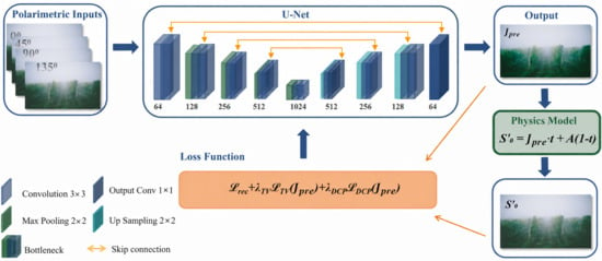
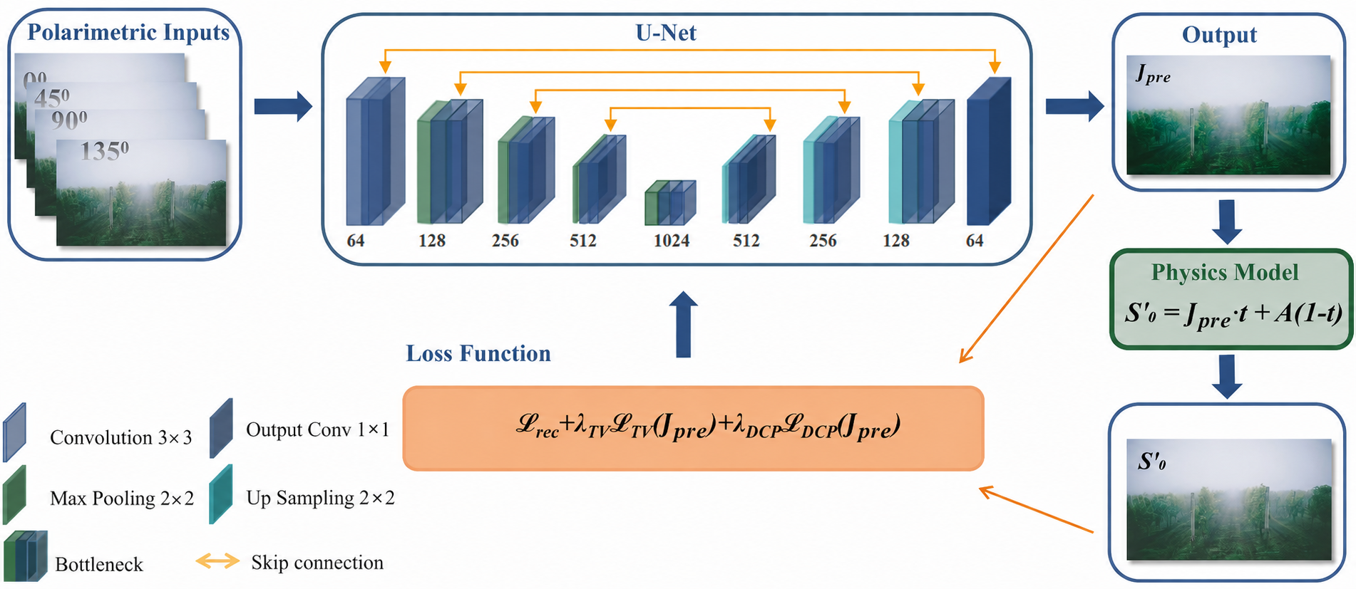
In this paper, U-Net was employed to predict the dehazed image. Its symmetric encoder–decoder architecture extracts multi-scale features, while the skip connections preserve spatial details that are important for image restoration [31]. These characteristics are suitable for dehazing, which requires both haze removal and structural detail preservation. As shown in Figure 2, the network takes as input four color images captured at rotating polarizer angles of 0°, 45°, 90°, and 135°, each with a resolution of 1024 × 768 pixels. The input data are concatenated along the channel dimension to form a multi-channel tensor, where the number of input channels given is by $C_{in}=3N_{angel}$. In the encoding stage, features are first extracted by a double-convolution block consisting of two 3 × 3 convolutions (stride 1), each followed by batch normalization and a ReLU. This is then followed by four downsampling modules, each comprising a max pooling operation and a double-convolution block, thereby halving the spatial resolution and doubling the number of channels at each stage. In the decoding stage, four upsampling modules are employed. Each module upsamples the feature map by a factor of 2 using a 2 × 2 transposed convolution (stride 2), concatenates it with the corresponding encoder features via a skip connection, and applies a double-convolution block for feature fusion and refinement. Finally, a 1 × 1 convolution maps the features to a $C_{out}=3$ color image, followed by Sigmoid activation to normalize pixel values to [0, 1], yielding the predicted dehazed image $J_{\mathit{pre}}$.

Figure 2. Overview of the physics-guided dehazing method based on polarization imaging.

To further improve the interpretability and generalization of the network in image dehazing, the loss function is designed with a physical-consistency constraint, which is derived from the atmospheric scattering model and polarization information, thereby ensuring that the dehazing process adheres to physical principles. In addition, regularization and statistical prior constraints are incorporated to suppress noise and artifacts during optimization [27,32]. The loss function is as follows:

$$L_{total}=L_{rec}+{{\lambda }_{TV}L}_{TV}(J_{pre})+{{\lambda }_{DCP}L}_{DCP}(J_{pre}),$$

(8)

where $L_{\mathit{rec}}$ denotes the reconstruction loss between the reconstructed total intensity S′₀, computed from the predicted dehazed image $J_{\mathit{pre}}$ using the atmospheric scattering model, and the observed total intensity $S_0$. It serves as the main physical-consistency constraint in the loss function. $L_{\mathit{TV}}$ denotes the total variation (TV) loss applied to the dehazed image $J_{\mathit{pre}}$, which suppresses noise and abrupt local intensity changes. The DCP loss $L_{\mathit{DCP}}$ denotes the dark channel prior loss computed from $J_{\mathit{pre}}$, which helps reduce residual haze and color distortion. ${\lambda }_{\mathit{TV}}$ and ${\lambda }_{\mathit{DCP}}$ denote the weighting parameters of $L_{\mathit{TV}}$ and $L_{\mathit{DCP}}$, respectively. The detailed design of each loss term will be described in the following subsections.

The intensity reconstruction loss is defined as the mean squared error (MSE) based on the L2 loss function, as follows:

$$L_{rec}={\displaystyle \frac{1}{N}}{‖{S^{\prime }}_0-S_0‖}_2^2,$$

(9)

where $N$ denotes the total number of pixels in the image. We first obtain initial estimates of $A$ and $t(x)$ from the four polarimetric input images using Equations (3)–(7). Next, using Equation (1), we compute S′₀ from the network’s prediction $J_{\mathit{pre}}$. On this basis, we further refine the estimates of $A$ and $t(x)$ via an optimization procedure. This procedure imposes a physical-consistency constraint on the network by minimizing the discrepancy between the reconstructed total intensity S′₀ and the observed total intensity $S_0$, thereby ensuring that the dehazing process conforms to the atmospheric scattering model.

However, in unsupervised optimization, relying solely on an L2 loss from the physical-consistency constraint tends to overfit noise and introduce artifacts. This is exacerbated by prolonged optimization without priors or regularization [33,34]. Accordingly, we introduce regularization and statistical prior constraints and jointly optimize them with the physical-consistency constraint to improve dehazed image quality. TV loss promotes gradient smoothness between neighboring pixels, preventing noise amplification due to oversharpening during dehazing, while preserving the natural smoothness of structures such as crop canopies and ground textures, thereby enhancing the visual consistency of dehazed images. The expression is as follows [35]:

$$L_{TV}(J_{pre})={\displaystyle \frac{1}{N}}{\sum }_{i,j,c}\left[{(J_{pre}^{(c)}(i+1,j)-J_{pre}^{(c)}(i,j))}^2+{(J_{pre}^{(c)}(i,j+1)-J_{pre}^{(c)}(i,j))}^2\right],$$

(10)

where $c$ denotes the color channel in the dehazed image.

The DCP loss leverages the statistical property of dehazed images, where in a local region at least one color channel contains dark pixels with intensities close to zero. Specifically, by constraining the dark channel characteristics of $J_{\mathit{pre}}$, the network can learn the intrinsic features of dehazed images without requiring ground-truth data, thereby effectively reducing residual haze and mitigating color distortion. The expression is as follows [36]:

$$L_{DCP}(J_{pre})={\displaystyle \frac{1}{N}}{\sum }_{i,j}\left[{min}_c({min}_{(p,q)\in {\Omega }_{i,j}}{J}_{pre}^{(c)}(p,q))\right],$$

(11)

where ${\Omega }_{i,j}$ denotes the local patch of size 15 × 15 centered at (i,j).

In summary, the proposed dehazing method can be trained using only four polarized images of the same scene acquired at four distinct angles of the rotating polarizer, without any additional training data. The resulting network exhibits a certain degree of physical interpretability.

2.4. Experimental Setup

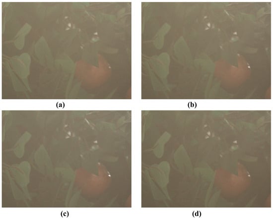
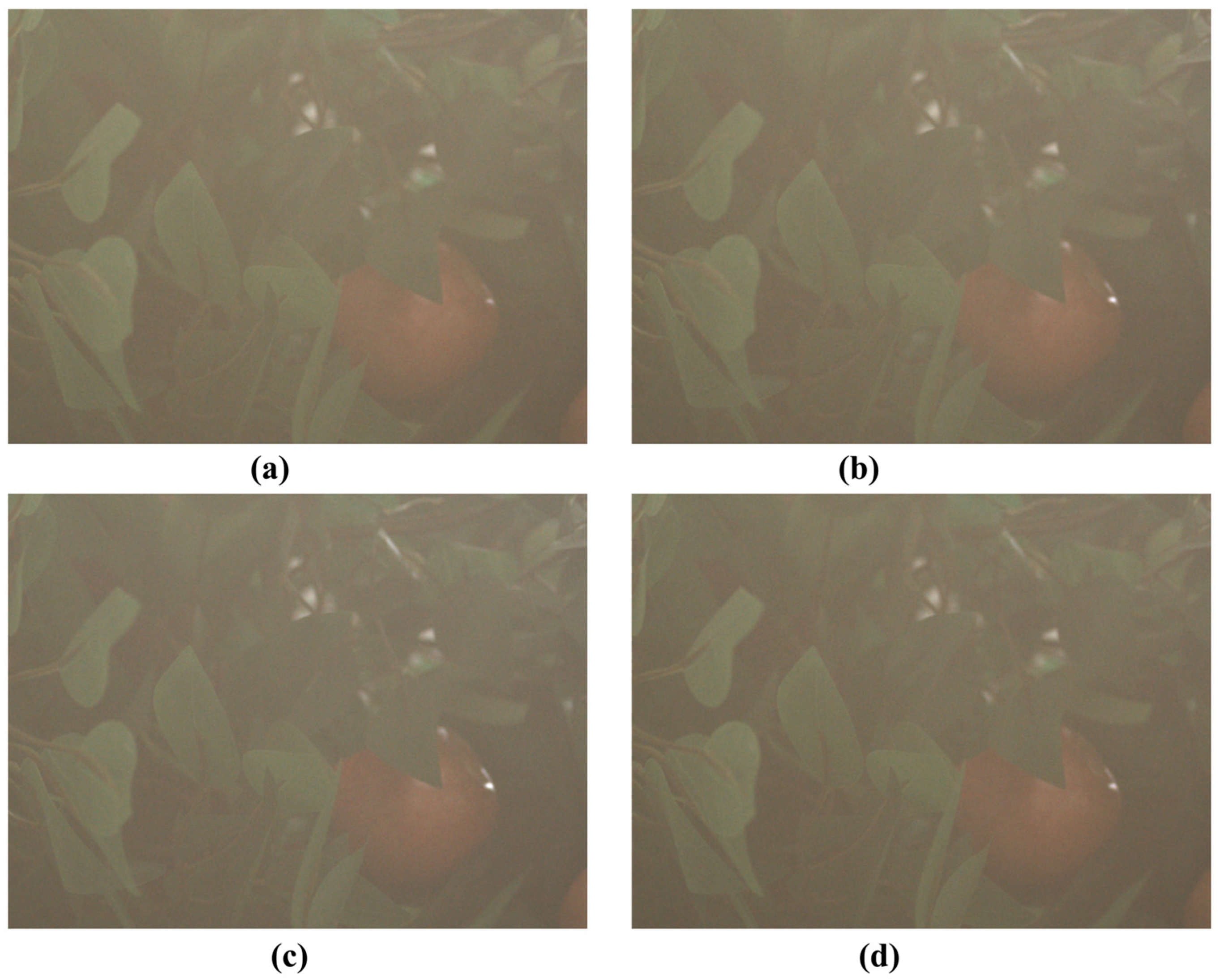
Two types of experimental data were used to evaluate the proposed method. First, real-world polarimetric hazy images were acquired using an MER2-503-23GC-P industrial camera with a resolution of 1024 × 768 pixels and fitted with a rotating polarizer. Color images were captured at four polarization angles 0°, 45°, 90°, and 135°for each scene. The dataset comprises diverse scenarios, including crops, mountainous vegetation, fruit trees, and village architecture, spanning both near- and far-field views. This diversity provides a solid basis for assessing the algorithm’s generalization ability and robustness. Figure 3 presents fruit tree images acquired at the four polarization angles.

Figure 3. Polarimetric images captured at four polarization angles: (a) 0°, (b) 45°, (c) 90°, and (d) 135°.

Second, to enable full-reference evaluation, two hazy/haze-free image pairs were selected from the real-world LMHaze dataset [37]. Since LMHaze provides conventional intensity images rather than polarimetric images, four polarimetric images at rotating polarizer angles of 0°, 45°, 90°, and 135° were synthesized from each hazy image using the polarization imaging model. Spatially varying P and θ were generated, with P constrained to 0.03–0.28. The corresponding haze-free images were used as the ground truth for quantitative evaluation.

To comprehensively evaluate the performance of different dehazing methods, both qualitative and quantitative evaluations were conducted. The qualitative evaluation was based on visual comparisons in terms of haze removal, color fidelity, and detail preservation. For quantitative evaluation, different metrics were used for the constructed paired polarimetric data and the real polarimetric hazy images. For the paired polarimetric data constructed from the LMHaze dataset, peak signal-to-noise ratio (PSNR), structural similarity index measure (SSIM), and the Fog Aware Density Evaluator (FADE) [38] were employed. PSNR and SSIM were used to compare the dehazed images with the corresponding haze-free ground-truth images, while FADE was used to estimate the remaining haze. For the real polarimetric hazy images, where aligned haze-free reference images were unavailable, contrast (C) [39], mean gradient (MG) [40], and FADE were used to evaluate image contrast, edge and texture details, and remaining haze, respectively. Higher PSNR and SSIM values indicate that the dehazed images are closer to the ground-truth images. Higher C and MG values generally indicate stronger contrast and clearer details, whereas a lower FADE value indicates less remaining haze.

In this paper, the neural network model was trained on a high-performance server equipped with an NVIDIA RTX A6000 GPU. All experiments were conducted using the PyTorch 2.5 deep learning framework, with source code written in Python 3.6.5. The Adam optimizer was employed with an initial learning rate of 1 × 10⁻⁴. Based on preliminary experiments, the TV and DCP weights were set to ${\lambda }_{\mathit{TV}}=1\times {10}^{-4}$ and ${\lambda }_{\mathit{DCP}}=5\times {10}^{-3}$, respectively. The training was performed for 500 epochs using a ReduceLROnPlateau scheduler to adaptively adjust the learning rate and enhance convergence stability.

3. Results and Discussion

To assess the performance of our method, we compared it with several representative dehazing methods, including the physical model-based DCP [4], the supervised convolutional network AOD [16], the Transformer-based DehazeFormer [17], the unsupervised method D4 [40], and Learning to Dehaze with Polarization (LDP) [41], using both qualitative and quantitative evaluations. To ensure a fair comparison, the traditional DCP method used the parameter settings reported in the original paper, whereas the deep learning-based methods, including AOD, DehazeFormer, D4, and LDP were evaluated using their official pretrained models. All methods were tested on the same scenes.

3.1. Evaluation on Synthetic Data

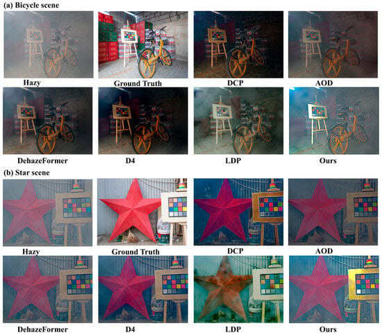
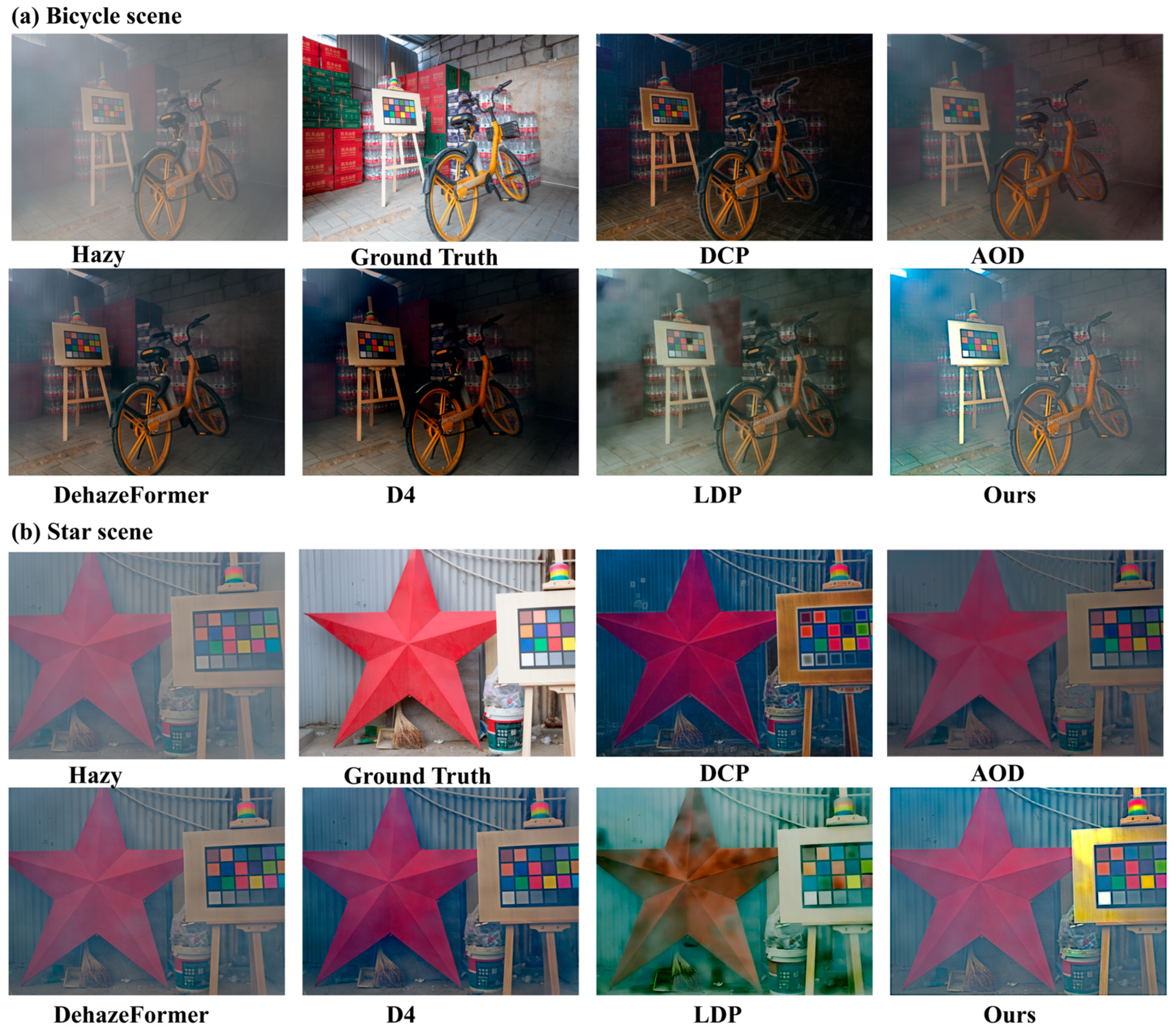
Comparative experiments were first conducted on the synthetic polarimetric data described in Section 2.4. As shown in Figure 4, the different methods exhibit noticeable differences in haze removal, color recovery, and detail preservation. DCP and D4 enhance image contrast, but their results are relatively dark, leading to detail loss in shadow regions. AOD and DehazeFormer alleviate part of the haze; however, residual haze remains, and the restored images exhibit insufficient contrast. LDP improves scene visibility by exploiting polarization information but introduces obvious color distortion and spatially nonuniform artifacts, particularly in the star scene. In comparison, the proposed method produces results that are visually closer to the corresponding ground-truth images, with more natural color recovery, clearer structural details, and fewer artifacts. Although slight brightness deviations remain in some local regions, the proposed method achieves a better overall balance among haze removal, color preservation, and detail recovery across both scenes.

Figure 4. Qualitative comparison of different dehazing methods on synthetic polarimetric data. (a) Bicycle scene and (b) star scene.

As shown in Table 1, the proposed method achieves the highest PSNR values in both scenes. For the (a) bicycle scene, it also obtains the highest SSIM and the lowest FADE. For the (b) star scene, DehazeFormer achieves the highest SSIM, while DCP obtains the lowest FADE. Nevertheless, the proposed method achieves the highest PSNR and the second-lowest FADE, demonstrating a favorable balance between reconstruction accuracy and haze removal.

Table 1. Quantitative comparison of different dehazing methods on synthetic data.

Method	(a) Bicycle Scene			(b) Star Scene
	PSNR ↑	SSIM ↑	FADE ↓	PSNR ↑	SSIM ↑	FADE ↓
DCP	7.9977	0.3609	1.0705	9.0512	0.5889	0.6058
AOD	10.2485	0.4838	1.6566	9.6170	0.6530	1.3963
DehazeFormer	9.8389	0.4963	1.6242	11.7781	0.7634	1.3755
D4	8.0705	0.3508	1.2849	11.1071	0.7446	0.8781
LDP	11.0038	0.5385	1.4774	12.6346	0.7361	0.9844
Ours	13.1160	0.5437	0.8368	13.2107	0.7268	0.6839

Note: Bold values indicate the best performance for each metric.

3.2. Evaluation on Real Data

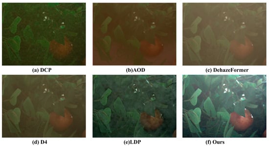
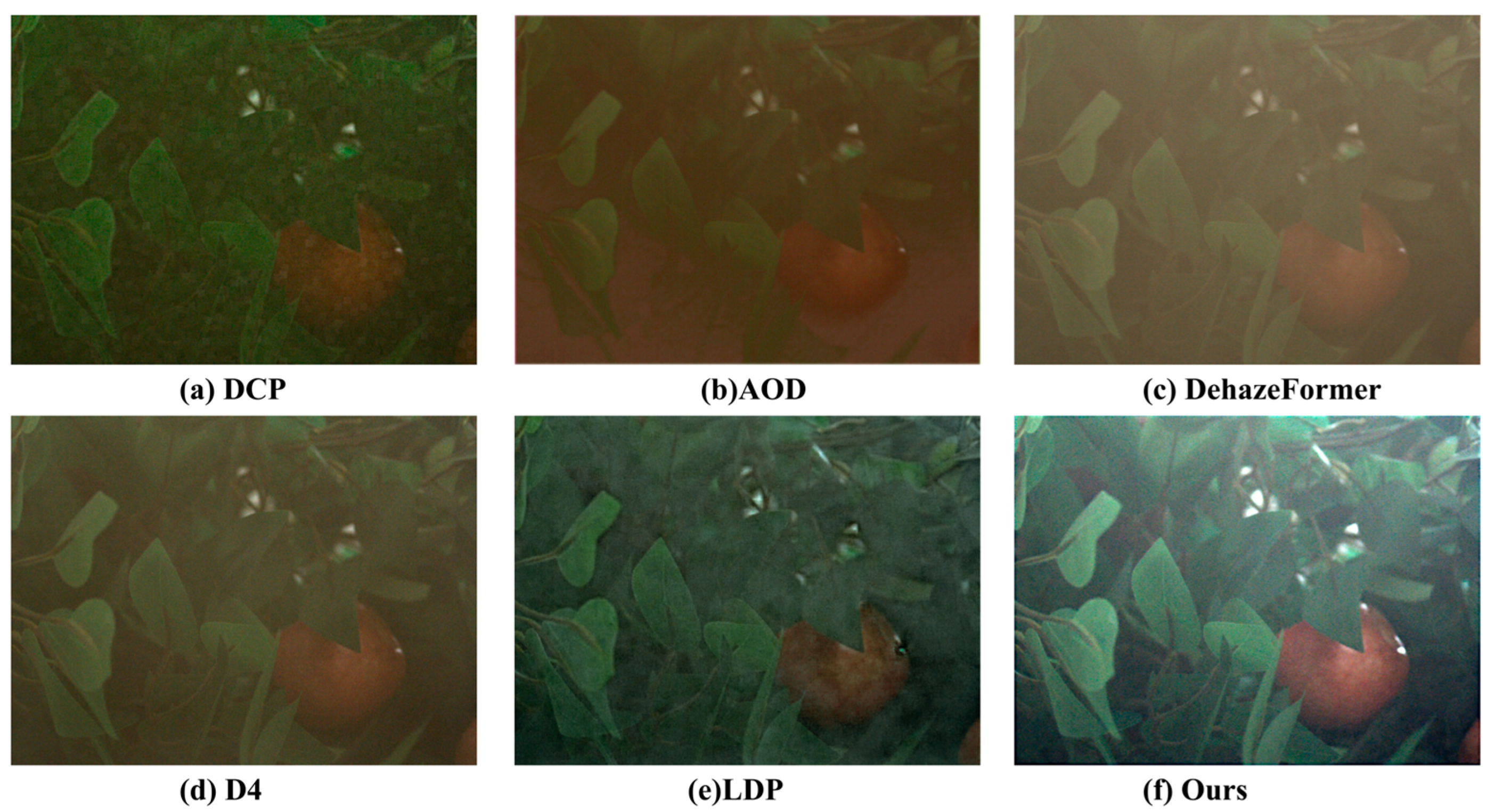
Following the evaluation on synthetic polarimetric data, the proposed method was further evaluated on real polarimetric hazy images. Since accurately haze-free reference images were unavailable for these scenes, the comparison was conducted through visual evaluation and the no-reference metrics C, MG, and FADE. The restoration results for the fruit-tree scene shown in Figure 3 are presented in Figure 5. DCP enhances local contrast but produces an excessively dark result, accompanied by noticeable color distortion and loss of details in shadow regions. AOD and D4 provide limited haze removal, and considerable residual haze remains, resulting in low contrast and unclear structural details. DehazeFormer increases the overall brightness; however, the restored image exhibits a yellowish color deviation, and some fine details remain blurred. LDP improves the visibility of leaves and fruits but produces a relatively dark result with evident color deviation. In comparison, the proposed method more effectively suppresses residual haze and restores clearer leaf contours and fruit details. Although slight color deviation and local over-enhancement remain, the proposed method achieves a better balance among haze removal, contrast enhancement, color preservation, and detail recovery.

Figure 5. Comparison of dehazing results in haze scenes using different methods. (a) DCP method, (b) AOD method, (c) DehazeFormer method, (d) D4 method, (e) LDP method and (f) our method.

Subsequently, quantitative analysis was conducted using the no-reference metrics C, MG, and FADE, and the results are presented in Table 2. Compared with the original hazy image, all dehazing methods increase C and MG while reducing FADE, indicating improvements in image contrast, detail visibility, and haze removal. DCP produces a large increase in MG and a substantial decrease in FADE, but its result in Figure 5 appears excessively dark and exhibits noticeable color distortion. AOD improves image contrast and details, whereas DehazeFormer shows relatively limited changes in all three metrics, which is consistent with the residual haze observed in Figure 5. Compared with AOD, D4 obtains a higher MG and a lower FADE, although its C value is slightly lower, indicating stronger detail enhancement and haze removal but more limited contrast improvement. LDP considerably increases C and MG; however, its FADE value remains relatively close to that of the original hazy image, suggesting that its improvement is mainly reflected in contrast and detail enhancement rather than haze removal. The proposed method achieves the highest C and MG values and the lowest FADE value among all evaluated methods, indicating simultaneous improvements in image contrast, detail visibility, and haze suppression. These quantitative results are consistent with the visual comparison in Figure 5.

Table 2. Comparison of image quality metrics for different dehazing methods.

	Hazy	DCP	AOD	DehazeFormer	D4	LDP	Ours
C ↑	0.0769	0.1732	0.1689	0.1045	0.1565	0.2502	0.3492
MG ↑	1.7952	3.4637	2.5514	2.1180	2.8303	3.0503	4.6746
FADE ↓	1.2199	0.6224	0.8786	0.8839	0.7762	1.0070	0.4443

Note: Bold values indicate the best performance for each metric.

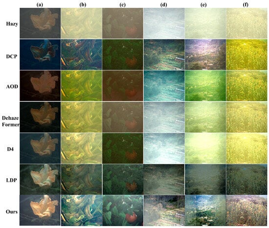
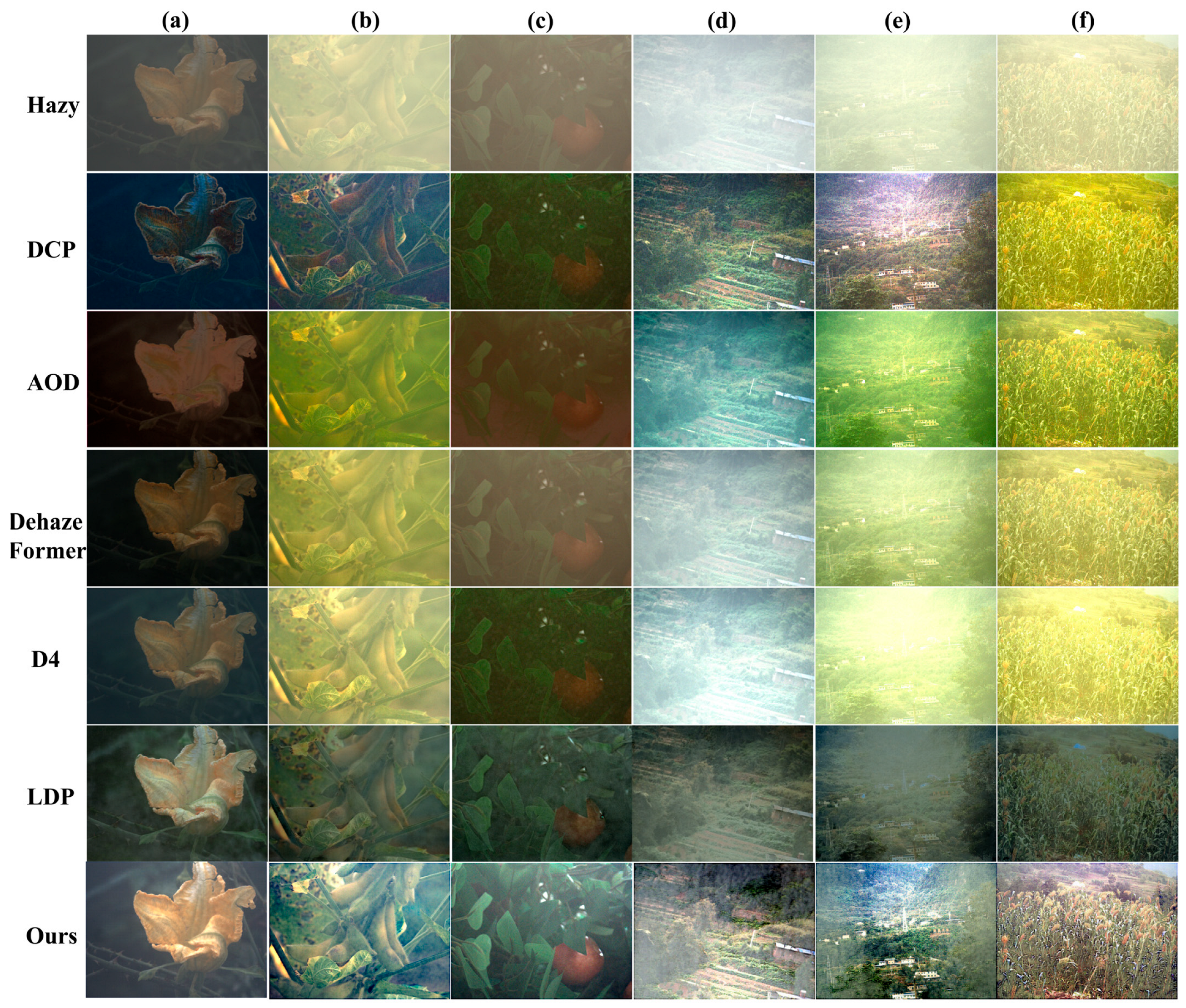
To further evaluate the robustness of our method across different scenes and haze conditions, we selected six real polarimetric hazy images, including close-range views of leaves and fruits and distant views of farmland and mountainous areas. The comparison results are presented in Figure 6. The original hazy images exhibit low contrast, noticeable color shifts, and blurred details, particularly in the distant scenes shown in Figure 6d–f. DCP enhances image contrast but often produces dark results, strong color shifts, and overly enhanced edges. AOD and DehazeFormer improve image visibility to some extent; however, residual haze and yellowish or greenish color shifts remain in several scenes. D4 provides limited improvement in the close-range scenes, while considerable haze remains in the distant scenes, resulting in unclear details. LDP improves the visibility of leaves, fruits, and distant objects, but its results are generally dark and show noticeable color differences across scenes. In comparison, our method more effectively reduces residual haze and restores clearer leaf contours, fruit textures, and details in distant farmland and mountainous areas. Although overly bright regions and slight color shifts remain in some scenes, our method achieves a better overall balance among haze removal, detail recovery, and color preservation across the six scenes.

Figure 6. Qualitative comparison of dehazing performance. (a) Pumpkin flower, (b) citrus, (c) soybean, (d) mountain terraces, (e) mountain village, and (f) sorghum field.

Our method employs a physical-consistency constraint derived from the atmospheric scattering model and polarization information to guide network learning. It requires only four polarization images of the same scene, captured at different rotating polarizer angles, to complete neural network training, thereby eliminating the reliance on large-scale training datasets and providing the network with a certain degree of interpretability. Experimental results indicate that, in real-world outdoor conditions, the image dehazing performance of our method surpasses that of commonly used deep learning-based methods. However, the method also faces several challenges. First, the accuracy of the physical model significantly affects the reconstruction results. If the selected model deviates from the actual scene, the dehazed images output by the network may still suffer from detail loss and color distortion. Second, polarimetric image acquisition is highly susceptible to interference from electronic noise, which can degrade image quality and consequently cause artifacts and other defects in the dehazed output.

3.3. Ablation Study of the Loss Function

To verify the contribution of each loss term, we used $L_{\mathit{rec}}$ as the baseline and added $L_{TV}$ and $L_{DCP}$ separately, resulting in four loss configurations. All configurations were evaluated under the same experimental settings. The quantitative results are presented in Table 3, and the corresponding visual results are shown in Figure 7.

Table 3. Ablation study of different loss terms on real polarimetric hazy image.

Lrec	LTV	LDCP	C ↑	MG ↑	FADE ↓
√			0.1639	2.2545	0.8936
√	√		0.1622	2.3051	0.9097
√		√	0.3636	5.7497	0.3761
√	√	√	0.3492	4.6746	0.4443

Note: Bold values indicate the best performance for each metric.

Figure 7. Visual comparison of different loss configurations on a real polarimetric hazy image. (a) Hazy image, (b) $L_{\mathit{rec}}$, (c) ${L_{\mathit{rec}}+{\lambda }_{\mathit{TV}}L}_{TV}$, (d) ${L_{\mathit{rec}}+{\lambda }_{DCP}L}_{DCP}$, and (e) the full loss.

As shown in Table 3, adding $L_{TV}$ alone produces only small changes in C, MG, and FADE, indicating that it does not directly improve haze removal. In contrast, adding $L_{DCP}$ substantially increases C and MG and reduces FADE, demonstrating its contribution to contrast enhancement and haze suppression. However, Figure 7d shows that using $L_{DCP}$ without $L_{TV}$ introduces noticeable noise, color shifts, and over-enhanced local regions. When $L_{TV}$ is combined with $L_{DCP}$, these problems are reduced, although the three metric values are slightly lower than those obtained using $L_{DCP}$ alone. These results indicate that $L_{DCP}$ mainly improves haze removal and image contrast, whereas $L_{TV}$ helps suppress noise and over-enhancement. Consequently, the full loss produces a more natural balance between haze removal and detail preservation.

3.4. Optimization Process Analysis

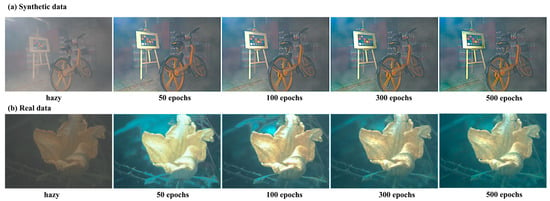
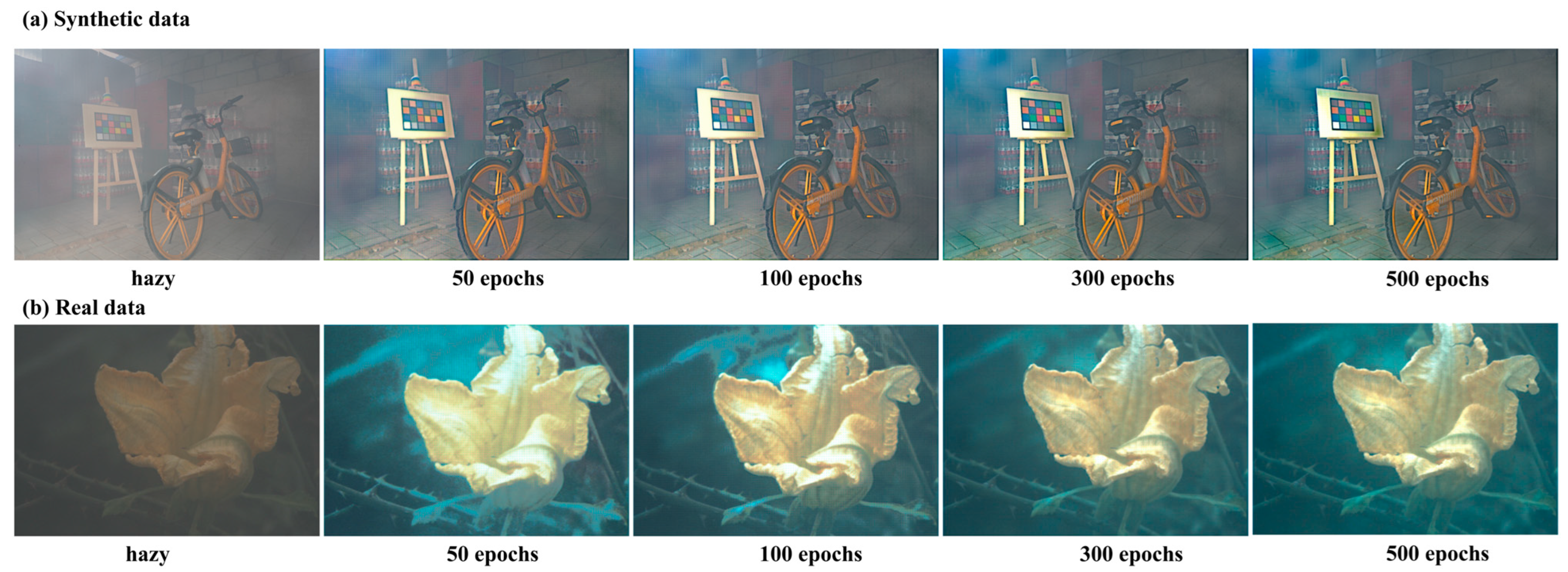
To examine the optimization process of the proposed method, Figure 8 presents the dehazing results obtained at different epochs. At epoch 100, residual haze remains in the image, particularly in the background. As the optimization proceeds, the residual haze is gradually reduced, while the image contrast and structural details of Figure 8a,b are improved. After epoch 300, the differences among the results become relatively small, indicating that the optimization is close to convergence. At epoch 500, the predicted dehazed image shows clearer structural details and more natural color recovery. These changes indicate that the physical-consistency constraint provided by $L_{rec}$, together with $L_{TV}$ and $L_{DCP}$, progressively guides the network output during optimization.

Figure 8. Evolution of the dehazing results during optimization.

4. Conclusions

This paper proposed a physics-guided dehazing method based on polarization imaging. The proposed method uses only four polarimetric images of the same scene acquired at distinct rotating polarizer angles, eliminating the need for large paired datasets while retaining physical interpretability. The experimental results show that it outperforms commonly used deep learning-based dehazing methods in both qualitative and quantitative evaluations. Furthermore, using a physical model to guide the neural network in generating high-quality dehazed images provides strong support for the further development and application of transportation, aviation, and environmental monitoring in complex, foggy environments, and opens up new avenues for the application of deep learning in image processing, optics, and related fields [2,3].

In the future, we will improve the dehazing performance by optimizing the physical model and integrating polarimetric image denoising. Specifically, we will conduct an in-depth analysis of the applicability of atmospheric scattering and related models. Meanwhile, polarimetric image denoising techniques will be integrated to suppress electronic noise and other interference, thereby providing the neural network with high-quality polarimetric inputs and improving the clarity and accuracy of the resulting dehazed images. Finally, the robustness of the proposed method to polarizer-angle errors will be further investigated. Controlled angular perturbations will be introduced to evaluate their effects on the Stokes parameter calculation, transmission estimation, and final dehazing performance.

References

- Israël, H.; Kasten, F. KOSCHMIEDERs Theorie der horizontalen Sichtweite. In Die Sichtweite im Nebel und Die Möglichkeiten Ihrer Künstlichen Beeinflussung; Springer: Berlin, Germany, 1959; pp. 7–10. [Google Scholar]
- Jiang, J.; Zuo, Z.; Wu, G.; Jiang, K.; Liu, X. A Survey on All-in-One Image Restoration: Taxonomy, Evaluation and Future Trends. IEEE Trans. Pattern Anal. Mach. Intell. 2025, 47, 11892–11911. [Google Scholar] [CrossRef] [Scilit] [PubMed]
- Yin, S.; Shi, Y.; Wang, Y.; Yang, Y.-H. When Aware Haze Density Meets Diffusion Model for Synthetic-to-Real Dehazing. IEEE Trans. Circuits Syst. Video Technol. 2025, 35, 4242–4255. [Google Scholar] [CrossRef] [Scilit]
- He, K.; Sun, J.; Tang, X. Single image haze removal using dark channel prior. IEEE Trans. Pattern Anal. Mach. Intell. 2011, 33, 2341–2353. [Google Scholar] [CrossRef] [Scilit] [PubMed]
- Meng, G.; Wang, Y.; Duan, J.; Xiang, S.; Pan, C. Efficient image dehazing with boundary constraint and contextual regularization. In Proceedings of the IEEE International Conference on Computer Vision (ICCV), Sydney, Australia, 1–8 December 2013; pp. 617–624. [Google Scholar]
- Zhu, Q.; Mai, J.; Shao, L. A fast single image haze removal algorithm using color attenuation prior. IEEE Trans. Image Process. 2015, 24, 3522–3533. [Google Scholar] [CrossRef] [Scilit] [PubMed]
- Sun, H.; Yao, Z.; Du, B.; Wan, J.; Ren, D.; Tong, L. Spatial–Frequency Residual-Guided Dynamic Perceptual Network for Remote Sensing Image Haze Removal. IEEE Trans. Geosci. Remote Sens. 2025, 63, 5612416. [Google Scholar] [CrossRef] [Scilit]
- Zhang, J.; Wang, X.; Yang, C.; Zhang, J.; He, D.; Song, H. Image dehazing based on dark channel prior and brightness enhancement for agricultural remote sensing images from consumer-grade cameras. Comput. Electron. Agric. 2018, 151, 196–206. [Google Scholar] [CrossRef] [Scilit]
- Yang, K.; Liu, F.; Liang, S.Y.; Xiang, M.; Han, P.; Liu, J.; Dong, X.; Wei, Y.; Wang, B.; Shimizu, K.; et al. Data-driven polarimetric imaging: A review. Opto-Electron. Sci. 2024, 3, 230042. [Google Scholar] [CrossRef] [Scilit]
- Wu, Q.; Wei, X.; Su, X.; Ma, L.; Cai, C. Polarization-based dehazing algorithm under dense hazy conditions. J. Appl. Phys. 2025, 138, 104903. [Google Scholar] [CrossRef] [Scilit]
- Liang, J.; Ren, L.; Liang, R. Low-pass filtering based polarimetric dehazing method for dense haze removal. Opt. Express 2021, 29, 28178–28189. [Google Scholar] [CrossRef] [Scilit] [PubMed]
- Schechner, Y.Y.; Narasimhan, S.G.; Nayar, S.K. Polarization-based vision through haze. Appl. Opt. 2003, 42, 511–525. [Google Scholar] [CrossRef] [Scilit] [PubMed]
- LeCun, Y.; Bengio, Y.; Hinton, G. Deep learning. Nature 2015, 521, 436–444. [Google Scholar] [CrossRef] [Scilit] [PubMed]
- Goodfellow, I.; Bengio, Y.; Courville, A. Deep Learning, 1st ed.; MIT Press: Cambridge, MA, USA, 2016. [Google Scholar]
- Cai, B.; Xu, X.; Jia, K.; Qing, C.; Tao, D. DehazeNet: An end-to-end system for single image haze removal. IEEE Trans. Image Process. 2016, 25, 5187–5198. [Google Scholar] [CrossRef] [Scilit] [PubMed]
- Li, B.; Peng, X.; Wang, Z.; Xu, J.; Feng, D. AOD-Net: All-in-one dehazing network. In Proceedings of the IEEE International Conference on Computer Vision (ICCV), Venice, Italy, 22–29 October 2017; pp. 4770–4778. [Google Scholar] [CrossRef] [Scilit]
- Song, Y.; He, Z.; Qian, H.; Du, X. Vision transformers for single image dehazing. IEEE Trans. Image Process. 2023, 32, 1927–1941. [Google Scholar] [CrossRef] [Scilit] [PubMed]
- Wang, W.; Yuan, X.; Wu, X.; Liu, Y. Fast Image Dehazing Method Based on Linear Transformation. IEEE Trans. Multimed. 2017, 19, 1142–1155. [Google Scholar] [CrossRef] [Scilit]
- Jiang, S.; Mei, Y.; Wang, P.; Liu, Q. Exposure difference network for low-light image enhancement. Pattern Recognit. 2024, 156, 110796. [Google Scholar] [CrossRef] [Scilit]
- Liu, Y.; Li, T.; Zhou, Z.; Ren, W.; Lin, W. Real-World Nighttime Image Dehazing via Bayesian-Based Fractional-Order Variational Model. IEEE Trans. Image Process. 2026, 35, 4673–4685. [Google Scholar] [CrossRef] [Scilit] [PubMed]
- Zhou, H.; Wang, Y.; Zhang, Q.; Tao, T.; Ren, W. A Dual-Stage Residual Diffusion Model with Perceptual Decoding for Remote Sensing Image Dehazing. IEEE Trans. Geosci. Remote Sens. 2025, 63, 4109312. [Google Scholar] [CrossRef] [Scilit]
- Simonyan, K.; Zisserman, A. Very deep convolutional networks for large-scale image recognition. arXiv 2015, arXiv:1409.1556. [Google Scholar]
- Szegedy, C.; Liu, W.; Jia, Y.; Sermanet, P.; Reed, S.; Anguelov, D.; Erhan, D.; Vanhoucke, V.; Rabinovich, A. Going deeper with convolutions. In Proceedings of the IEEE Conference on Computer Vision and Pattern Recognition, Boston, MA, USA, 7–12 June 2015; pp. 1–9. [Google Scholar] [CrossRef] [Scilit]
- Chen, Z.; He, Z.; Lu, Z.M. DEA-net: Single image dehazing based on detail-enhanced convolution and content-guided attention. IEEE Trans. Image Process. 2024, 33, 1002–1015. [Google Scholar] [CrossRef] [Scilit] [PubMed]
- Li, B.; Gou, Y.; Gu, S.; Liu, J.Z.; Zhou, J.T.; Peng, X. You only look yourself: Unsupervised and untrained single image dehazing neural network. Int. J. Comput. Vis. 2021, 129, 1754–1767. [Google Scholar] [CrossRef] [Scilit]
- Zhang, S.; Zhang, X.; Wan, S.; Ren, W.; Zhao, L.; Shen, L. Generative adversarial and self-supervised dehazing network. IEEE Trans. Ind. Inform. 2024, 20, 4187–4197. [Google Scholar] [CrossRef] [Scilit]
- Bi, P.; Wang, D.; Chen, W.; Yang, L.; Liang, J.; Li, G.; Zhang, F.; Wang, Z.; Zhang, X. Image dehazing based on polarization information and deep prior learning. Optik 2022, 267, 169746. [Google Scholar] [CrossRef] [Scilit]
- Narasimhan, S.G.; Nayar, S.K. Contrast restoration of weather degraded images. IEEE Trans. Pattern Anal. Mach. Intell. 2003, 25, 713–724. [Google Scholar] [CrossRef] [Scilit]
- Pandey, P.; Gupta, R.; Goel, N. Comprehensive review of single image defogging techniques: Enhancement, prior, and learning based approaches. Artif. Intell. Rev. 2025, 58, 116. [Google Scholar] [CrossRef] [Scilit]
- Goldstein, D.H. Chapter 5: Stokes Polarization Parameters. In Polarized Light, 3rd ed.; Chemical Rubber Company: Cleveland, OH, USA, 2017; pp. 60–77. [Google Scholar]
- Ronneberger, O.; Fischer, P.; Brox, T. U-Net: Convolutional Networks for Biomedical Image Segmentation. In Medical Image Computing and Computer-Assisted Intervention—MICCAI 2015; Navab, N., Hornegger, J., Wells, W., Frangi, A., Eds.; Lecture Notes in Computer Science; Springer: Cham, Switzerland, 2015; Volume 9351, pp. 234–241. [Google Scholar] [CrossRef] [Scilit]
- Li, B.; Gou, Y.; Liu, J.Z.; Zhu, H.; Zhou, J.T.; Peng, X. Zero-Shot Image Dehazing. IEEE Trans. Image Process. 2020, 29, 8457–8466. [Google Scholar] [CrossRef] [Scilit] [PubMed]
- Ulyanov, D.; Vedaldi, A.; Lempitsky, V. Deep Image Prior. In Proceedings of the IEEE Conference on Computer Vision and Pattern Recognition (CVPR), Salt Lake City, UT, USA, 18–23 June 2018; pp. 9446–9454. [Google Scholar]
- Rudin, L.I.; Osher, S.; Fatemi, E. Nonlinear total variation based noise removal algorithms. Phys. D Nonlinear Phenom. 1992, 60, 259–268. [Google Scholar] [CrossRef] [Scilit]
- Golts, A.; Freedman, D.; Elad, M. Unsupervised single image dehazing using dark channel prior loss. IEEE Trans. Image Process. 2019, 29, 2692–2701. [Google Scholar] [CrossRef] [Scilit] [PubMed]
- Zhang, R.; Yang, H.; Yang, Y.; Fu, Y.; Pan, L. LMHaze: Intensity-aware Image Dehazing with a Large-scale Multi-intensity Real Haze Dataset. In Proceedings of the 6th ACM International Conference on Multimedia in Asia–MMAsia 2024, Auckland, New Zealand, 3–6 December 2024; ACM: New York, NY, USA, 2024; Article No. 18. [Google Scholar]
- Choi, L.K.; You, J.; Bovik, A.C. Referenceless prediction of perceptual fog density and perceptual image defogging. IEEE Trans. Image Process. 2015, 24, 3888–3901. [Google Scholar] [CrossRef] [Scilit] [PubMed]
- Liang, J.; Ren, L.; Ju, H.; Zhang, W.; Qu, E. Polarimetric dehazing method for dense haze removal based on distribution analysis of angle of polarization. Opt. Express 2015, 23, 26146–26157. [Google Scholar] [CrossRef] [Scilit] [PubMed]
- Wang, W.; Yuan, X. Recent advances in image dehazing. IEEE/CAA J. Autom. Sin. 2017, 4, 410–436. [Google Scholar] [CrossRef] [Scilit]
- Yang, Y.; Wang, C.; Liu, R.; Zhang, L.; Guo, X.; Tao, D. Self-augmented unpaired image dehazing via density and depth decomposition. In Proceedings of the IEEE/CVF Conference on Computer Vision and Pattern Recognition (CVPR), New Orleans, LA, USA, 19–24 June 2022; pp. 2037–2046. [Google Scholar]
- Zhou, C.; Teng, M.; Han, Y.; Xu, C.; Shi, B. Learning to dehaze with polarization. In Proceedings of the Advances in Neural Information Processing Systems (NeurIPS), Virtual, 6–14 December 2021. [Google Scholar]
Disclaimer/Publisher’s Note: The statements, opinions and data contained in all publications are solely those of the individual author(s) and contributor(s) and not of MDPI and/or the editor(s). MDPI and/or the editor(s) disclaim responsibility for any injury to people or property resulting from any ideas, methods, instructions or products referred to in the content. |
© 2026 by the authors. Licensee MDPI, Basel, Switzerland. This article is an open access article distributed under the terms and conditions of the Creative Commons Attribution (CC BY) license.