Landau–Zener–Stückelberg–Majorana Interference in Optical Resonators: A Temporal Coupled-Mode Theory Approach

Abstract

Landau–Zener–Stückelberg–Majorana (LZSM) interference describes the coherent superposition of nonadiabatic transitions when a quantum system is driven through an avoided crossing, but its classical optical analog remains largely unexplored. This work establishes an optical-resonator-based platform for exploring LZSM interference in atomic polarization dynamics using temporal coupled-mode theory. By exploiting the formal correspondence between the cavity mode and atomic polarization in a weakly driven two-level system (TLS), exact analytical solutions are derived for linear frequency sweeps and sinusoidal modulation. The results reveal that the Landau–Zener transition of atomic polarization occurs even when the input frequency transiently sweeps across resonance. The finite temporal memory inherent in the cavity response gives rise to Stückelberg interference, manifesting as oscillations in transmission and cavity energy. The dependence of the interference pattern on sweep rate, linewidth, and modulation is systematically analyzed, and a non-monotonic behavior of oscillation amplitude versus the cavity linewidth is identified. Furthermore, the conventional critical coupling concept is reexamined in the nonadiabatic regime, where counterintuitively the deepest transmission dip occurs under over-coupling rather than critical coupling. Finally, an inverse-design approach engineering both the amplitude and frequency of the input frequency is introduced to tailor the LZSM interference pattern. Our results provide a new platform to all-optical simulation of complex quantum interference.

1. Introduction

Landau–Zener–Stückelberg–Majorana (LZSM) interference describes the coherent superposition of nonadiabatic transitions when a quantum system is driven through an avoided crossing [1,2,3,4,5,6,7,8,9,10]. It has been extensively studied in diverse physical platforms, including superconducting qubits [11,12,13,14], cold atoms and molecules [15,16,17,18,19,20], quantum dots [21,22,23,24,25], solid-state defects [26,27,28,29,30], topological photonics [31,32,33] and optomechanics [34,35]. Conventional LZSM theories focus primarily on level populations, as population readout is natural in many quantum information contexts. However, in several atom–field interaction systems, experimental observations increasingly focus on atomic polarization [36,37,38,39,40,41,42,43]. This quantity carries both amplitude and phase information, governs the optical absorption and dispersion of the medium, and is naturally measured via interferometric techniques [44,45,46]. Moreover, its dephasing time is typically much shorter than the population relaxation time, facilitating the observation of fast transient dynamics that are inaccessible in population measurements. These considerations naturally raise the question of whether the characteristic LZSM interference, conventionally associated with population dynamics, can also emerge in the evolution of atomic polarization.

Optical resonators have achieved significant success in simulating quantum optical phenomena such as Rabi oscillation [47], electromagnetically induced transparency (EIT) [48,49], and electromagnetically induced absorption (EIA) [50], where atomic polarization plays a central role. Temporal coupled-mode theory (TCMT) provides a simple yet powerful description of optical resonators [51,52,53]. In this theory, the cavity field obeys a first-order linear differential equation that is mathematically isomorphic to the evolution equation of atomic polarization in a two-level system (TLS) under the weak excitation approximation. This isomorphism suggests that an optical resonator can serve as a classical platform to emulate LZSM interference. Existing studies of transient responses in optical ring resonators have mainly relied on round-trip series expansion methods [54,55], which are well suited for describing distributed field propagation. However, these methods primarily focus on the round-trip evolution of optical fields at specific points, and their connection to the dynamics of atomic coherence is not explicit. Consequently, it remains desirable to establish an analytical framework that directly connects nonadiabatic cavity dynamics with LZSM interference in atomic polarization.

In this work, we explore LZSM interference from the perspective of atomic polarization by exploiting the analogy between optical resonators and weakly driven TLS. By temporal coupled-mode theory and the mapping between cavity mode and atomic polarization, we establish an atomic polarization-based framework for investigating LZSM dynamics in optical ring resonators. Within this framework, we derive exact analytical solutions for both linear frequency sweeps and sinusoidal modulation. These analytical results demonstrate that Landau–Zener transitions can be manifested in atomic polarization dynamics when the input frequency sweeps through resonance, and that temporal memory arising from the cavity response gives rise to Stückelberg interference, observed as oscillations in transmission and intracavity energy with a non-monotonic dependence on cavity linewidth. We further reexamine the critical coupling concept in the nonadiabatic regime, revealing that the deepest transmission dip counterintuitively occurs under over-coupling rather than critical coupling. Finally, we introduce an inverse-design approach that tailors the nonadiabatic response by engineering the amplitude and frequency of the input field, enabling the recovery of adiabatic Lorentzian transmission lineshapes. These results provide an all-optical platform for exploring nonadiabatic interference phenomena beyond conventional population-based measurements.

2. Theoretical Models

2.1. LZSM Interference in Atomic Polarization Picture

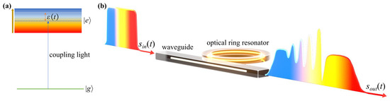
We consider a TLS with diabatic ground state $|g⟩$ and excited state $|e⟩$, shown in Figure 1a. The resonant angular frequency ${\omega }_0\left(t\right)$ of the TLS is time-dependent, and the laser interacting with the TLS has a constant angular frequency of ${\omega }_L$ and a constant Rabi frequency of g. Under the rotating wave approximation, the Hamiltonian in the Schrödinger picture can be written as

$$H^S=-{\displaystyle \frac{\hslash \Delta \left(t\right)}{2}}{\sigma }_z-{\displaystyle \frac{\hslash g}{2}}{\sigma }_x,$$

(1)

where $\Delta \left(t\right)={\omega }_0\left(t\right)-{\omega }_L$ is the detuning and the Pauli matrices are defined as

$${\sigma }_x=\left[\begin{array}{cc}0& 1\\ 1& 0\end{array}\right],{\sigma }_y=\left[\begin{array}{cc}0& -i\\ i& 0\end{array}\right],{\sigma }_z=\left[\begin{array}{cc}1& 0\\ 0& -1\end{array}\right],$$

(2)

with the basis states $|g⟩$ and $|e⟩$ represented by vectors ${\left[\begin{array}{cc}1& 0\end{array}\right]}^T$ and ${\left[\begin{array}{cc}0& 1\end{array}\right]}^T$, respectively. To establish a direct correspondence between atomic coherence dynamics and the evolution of a classical resonator mode, we describe the TLS in the Heisenberg picture. In this picture, the evolution of operators follows dynamical equations analogous to those of classical field amplitudes, meaning the Pauli matrices become time-dependent and can be expressed as

$${\sigma }_{x,y,z}^H\left(t\right)=U^{†}\left(t\right){\sigma }_{x,y,z}U\left(t\right),$$

(3)

where the unitary evolution operator is defined as

$$U\left(t\right)=\mathcal{T}{e}^{-{\displaystyle \frac{i}{\hslash }}{\int }_{t_0}^t{H}^S\left(t^{\prime }\right)d{t}^{\prime }}.$$

(4)

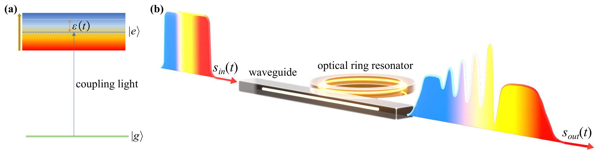
Figure 1. The illustrations of the LZSM inteference in a TLS (a) and an optical ring resonator coupled to a waveguide (b). In (a), $\epsilon \left(t\right)$ is the time-varying energy bias in a rotating frame. In (b), a quasi-continuous field with linear frequency sweep is incident into the system.

Here, $\mathcal{T}$ denotes the time-ordering operator, which arranges operators at later times to the left of those at earlier times, and $t_0$ is the initial time. Following a similar transformation, the Hamiltonian in the Heisenberg picture is given by $H^H\left(t\right)=U^{†}\left(t\right)H^{S}U\left(t\right)$ and is expressed as

$$H^H\left(t\right)=-{\displaystyle \frac{ϵ\left(t\right)}{2}}{\sigma }_z^H\left(t\right)-{\displaystyle \frac{G}{2}}{\sigma }_x^H\left(t\right).$$

(5)

At this point, we replace $\hslash \Delta \left(t\right)$ and $\hslash g$ with the energy bias $ϵ\left(t\right)$ and coupling strength G, which are more preferred in studies of LZSM interference [2]. The Heisenberg equation

$${\displaystyle \frac{d{\sigma }_{x,y,z}^H\left(t\right)}{dt}}={\displaystyle \frac{i}{\hslash }}[H^H\left(t\right),{\sigma }_{x,y,z}^H\left(t\right)],$$

(6)

is then employed to study the time evolution of the Pauli matrices. The Bloch vector of the TLS can be defined as ${[u\left(t\right),v\left(t\right),w\left(t\right)]}^T$, with each component representing the ensemble average of the corresponding Pauli matrix, namely, $u\left(t\right)=⟨{\sigma }_x^H\left(t\right)⟩$, $v\left(t\right)=⟨{\sigma }_y^H\left(t\right)⟩$ and $w\left(t\right)=⟨{\sigma }_z^H\left(t\right)⟩$. Substituting Equation (5) and the definition of the Bloch vector into Equation (6), and introducing relaxation phenomenologically [56], we obtain

$$\begin{array}{cc}\hfill {\displaystyle \frac{du\left(t\right)}{dt}}& =-{\displaystyle \frac{u\left(t\right)}{T_2}}+{\displaystyle \frac{ϵ\left(t\right)}{\hslash }}v\left(t\right),\hfill \\ \hfill {\displaystyle \frac{dv\left(t\right)}{dt}}& =-{\displaystyle \frac{v\left(t\right)}{T_2}}-{\displaystyle \frac{ϵ\left(t\right)}{\hslash }}u\left(t\right)+{\displaystyle \frac{G}{\hslash }}w\left(t\right),\hfill \\ \hfill {\displaystyle \frac{dw\left(t\right)}{dt}}& =-{\displaystyle \frac{w\left(t\right)-w_{eq}}{T_1}}-{\displaystyle \frac{G}{\hslash }}v\left(t\right),\hfill \end{array}$$

(7)

where $T_1$ and $T_2$ are the population relaxation time and the dephasing time, respectively, and $w_{eq}$ is the equilibrium population inversion.

The atomic polarization can be constructed via $p\left(t\right)=u\left(t\right)+iv\left(t\right)$ to describe the coherence in the TLS. Assuming that only the ground state is populated at equilibrium and applying the weak-excitation limit, the evolution equation for $p\left(t\right)$ simplifies to

$${\displaystyle \frac{dp\left(t\right)}{dt}}=-\left[{\displaystyle \frac{1}{T_2}}+i{\displaystyle \frac{ϵ\left(t\right)}{\hslash }}\right]p\left(t\right)-i{\displaystyle \frac{G}{\hslash }}.$$

(8)

Assuming the system starts in the ground state at $t\to -\infty$, i.e., $p(-\infty )=0$, we can express the solution of Equation (8) as

$$p\left(t\right)=-i{\displaystyle \frac{G}{\hslash }}{\int }_{-\infty }^t{e}^{-{\int }_{\tau }^t\left[{\displaystyle \frac{1}{T_2}}+i{\displaystyle \frac{ϵ\left(s\right)}{\hslash }}\right]ds}d\tau .$$

(9)

This expression represents a convolution of the driving term $-iG/\hslash$ with the memory kernel

$$K(t,\tau )=e^{-{\int }_{\tau }^t\left[{\displaystyle \frac{1}{T_2}}+i{\displaystyle \frac{ϵ\left(s\right)}{\hslash }}\right]ds}.$$

(10)

The convolution form reveals the memory effect of the system, wherein the atomic polarization retains a memory of the energy bias history $\epsilon \left(t\right)$ that is exponentially weighted by the dephasing time $T_2$ and the accumulated phase.

This memory effect is essential for LZSM interference. Each time the system passes through the avoided crossing, it acquires a phase that depends on the entire preceding trajectory. When the bias is modulated periodically, the interference between different passages is encoded in the convolution integral, leading to constructive or destructive superposition of the atomic polarization amplitude. Thus, the atomic polarization picture naturally captures the essence of Stückelberg oscillations as a history-dependent interference phenomenon.

2.2. Optical Analog of LZSM Interference in a Waveguide-Coupled Ring Resonator

We consider a single-mode ring resonator coupled to a straight waveguide, as illustrated in Figure 1b. The resonator supports a discrete cavity mode with resonant frequency ${\omega }_c$ and total decay rate $\mathsf{\Gamma }={\gamma }_i+{\gamma }_e$, where ${\gamma }_i$ accounts for intrinsic losses and ${\gamma }_e$ for the coupling to the waveguide. The cavity field amplitude $a\left(t\right)$ obeys the temporal coupled-mode equation [57]

$${\displaystyle \frac{da}{dt}}=-(i{\omega }_c+\mathsf{\Gamma })a-\sqrt{2{\gamma }_e}{s}_{\mathrm{in}}\left(t\right),$$

(11)

where $s_{\mathrm{in}}\left(t\right)$ is the input field. The output field from the straight waveguide is given by the input–output relationship [57]

$$s_{\mathrm{out}}\left(t\right)=s_{\mathrm{in}}\left(t\right)+\sqrt{2{\gamma }_e}a\left(t\right).$$

(12)

Physically, the input field excites the cavity mode, which subsequently re-radiates into the waveguide. The interference between the directly transmitted field and the re-radiated field determines the output. This configuration represents a coupled system with both continuum and bound states.

In a rotating frame, we can define $a\left(t\right)=\tilde{a}\left(t\right)e^{-i{\omega }_{0}t}$ and $s_{\mathrm{in}}\left(t\right)={\tilde{s}}_{\mathrm{in}}\left(t\right)e^{-i{\omega }_{0}t}$, where $\tilde{a}\left(t\right)$ and ${\tilde{s}}_{\mathrm{in}}\left(t\right)$ are the slowly varying envelopes of the cavity mode and input field with a central angular frequency of ${\omega }_0$. Substituting these two transformations into Equation (11), we obtain

$${\displaystyle \frac{d\tilde{a}}{dt}}=(i\Delta -\mathsf{\Gamma })\tilde{a}-\sqrt{2{\gamma }_e}{\tilde{s}}_{\mathrm{in}}\left(t\right),$$

(13)

where $\Delta ={\omega }_0-{\omega }_c$ is the detuning between the input field and the optical resonator. Equations (8) and (13) clearly share a highly similar mathematical form. A key insight for establishing the analogy with the LZSM problem is that the cavity mode amplitude in Equation (13) can be treated as a mathematical analogue of the atomic polarization in Equation (8) and Equation (13) can be solved explicitly as a convolution. For an arbitrary input ${\tilde{s}}_{\mathrm{in}}\left(t\right)$ and a zero initial condition $\tilde{a}\left(t\right)=0$, the solution is

$$\tilde{a}\left(t\right)=-\sqrt{2{\gamma }_e}{\int }_{-\infty }^t{e}^{(i\Delta -\mathsf{\Gamma })(t-t^{\prime })}{\tilde{s}}_{\mathrm{in}}\left(t^{\prime }\right)d{t}^{\prime }.$$

(14)

The cavity mode is thus the convolution of the input with a complex exponential memory kernel $h(t-t^{\prime })=\sqrt{2{\gamma }_e}{e}^{(i\Delta -\mathsf{\Gamma })(t-t^{\prime })}\mathsf{\Theta }(t-t^{\prime })$, where $\mathsf{\Theta }\left(\tau \right)$ is the Heaviside step function. The slowly varying part of the output field then becomes

$${\tilde{s}}_{\mathrm{out}}\left(t\right)={\tilde{s}}_{\mathrm{in}}\left(t\right)-2{\gamma }_e{\int }_{-\infty }^t{e}^{(i\Delta -\mathsf{\Gamma })(t-t^{\prime })}{\tilde{s}}_{\mathrm{in}}\left(t^{\prime }\right)d{t}^{\prime }.$$

(15)

This history-dependent form—where the output depends on the entire history of the input—is the precise analog of the atomic polarization dynamics in the LZSM problem, where the atomic polarization at time t depends on the entire history of the applied field via a convolution with a memory kernel determined by the atomic relaxation. This effect is also responsible for the conventional cavity buildup and decay dynamics observed when the input signal is switched on or off [58].

In the LZSM problem, the system itself is modulated; i.e., the energy bias $\epsilon \left(t\right)$ varies in time. In an optical resonator, however, the system is static and the modulation is applied to the input field. This distinction is physically crucial due to the fact that it is far easier to modulate the laser frequency than to rapidly tune a cavity resonance. Nevertheless, despite these structural differences, the two systems are mathematically equivalent if the input field of the optical resonator has a time-dependent phase while keeping its amplitude constant.

We first consider a linear frequency sweep through resonance to construct the optical analog of the Landau–Zener transition. In this case, the input phase is

$$\phi \left(t\right)={\omega }_{0}t+{\displaystyle \frac{\alpha }{2}}{(t-t_0)}^2,$$

(16)

where $\alpha$ is the sweep rate and $t_0$ is the time when the instantaneous angular frequency reaches ${\omega }_0$. In the rotating frame defined above, the input envelope becomes ${\tilde{s}}_{\mathrm{in}}\left(t\right)=e^{-i{\displaystyle \frac{\alpha }{2}}{(t-t_0)}^2}$. In an ideal single-pass frequency sweep, $\Delta$ can be arbitrary and here we assume $\Delta =0$ for simplicity. Substituting this assumption and the expression for ${\tilde{s}}_{\mathrm{in}}\left(t\right)$ into the convolution integral in Equation (14) yields

$$\tilde{a}\left(t\right)=-\sqrt{2{\gamma }_e}{\int }_{-\infty }^t{e}^{-\mathsf{\Gamma }(t-t^{\prime })}{e}^{-i{\displaystyle \frac{\alpha }{2}}{(t^{\prime }-t_0)}^2}d{t}^{\prime }.$$

(17)

This integral can be evaluated exactly as (see the details in the Supplementary Materials)

$$\begin{array}{cc}\hfill \tilde{a}\left(t\right)=-& \sqrt{2{\gamma }_e}\sqrt{{\displaystyle \frac{\pi }{i\alpha }}}{e}^{-\mathsf{\Gamma }(t-t_0)}{e}^{-{\displaystyle \frac{{\mathsf{\Gamma }}^2}{2i\alpha }}}\hfill \\ & \times {\displaystyle \frac{1+\mathrm{erf}\left(\sqrt{\frac{i\alpha }{2}}\left(t-t_0+\frac{i\mathsf{\Gamma }}{\alpha }\right)\right)}{2}},\hfill \end{array}$$

(18)

where $\mathrm{erf}\left(z\right)$ is the error function of a complex argument. This solution explicitly shows how the cavity field builds up as the sweep passes through resonance. According to Equation (12), the output intensity can then be obtained as $I_{\mathrm{out}}\left(t\right)=|{\tilde{s}}_{\mathrm{out}}{\left(t\right)|}^2={|{\tilde{s}}_{\mathrm{in}}\left(t\right)+\sqrt{2{\gamma }_e}\tilde{a}\left(t\right)|}^2$, and the transmission can be defined as $T\left(t\right)=I_{\mathrm{out}}\left(t\right)/{\left|{\tilde{s}}_{\mathrm{in}}\left(t\right)\right|}^2$, which is exactly $I_{\mathrm{out}}\left(t\right)$ if the input field has unit intensity.

Next, we consider a sinusoidal frequency modulation, which is the direct analog of periodic LZSM driving, in order to capture the optical analog of Stückelberg-like oscillations. In this case, the phase of the input signal is $\phi \left(t\right)={\omega }_{0}t+A\sin \left(\mathsf{\Omega }t\right)/\mathsf{\Omega }$, where A is the modulation depth and $\mathsf{\Omega }$ is the modulation frequency. The instantaneous angular frequency is ${\omega }_{\mathrm{in}}\left(t\right)={\omega }_0+A\cos \left(\mathsf{\Omega }t\right)$, and the input envelope becomes ${\tilde{s}}_{\mathrm{in}}\left(t\right)=e^{-iA\sin \left(\mathsf{\Omega }t\right)/\mathsf{\Omega }}$ when transformed to a frame rotating at an angular frequency of ${\omega }_0$. Using the Jacobi–Anger expansion $e^{-iA\sin \left(\mathsf{\Omega }t\right)/\mathsf{\Omega }}={\sum }_{k=-\infty }^{\infty }{J}_k(A/\mathsf{\Omega })e^{-ik\mathsf{\Omega }t}$ and substituting it into the convolution integral in Equation (14), we can express the convolution as a series summation

$$\tilde{a}\left(t\right)=-\sqrt{2{\gamma }_e}{\displaystyle \sum _{k=-\infty }^{\infty }}{J}_k\left({\displaystyle \frac{A}{\mathsf{\Omega }}}\right){\displaystyle \frac{e^{-ik\mathsf{\Omega }t}}{i(\Delta +k\mathsf{\Omega })-\mathsf{\Gamma }}}.$$

(19)

This solution has a clear physical interpretation. The input field generates a series of frequency sidebands, each of which can resonantly excite the cavity mode when its frequency matches the cavity resonance (i.e., $\Delta +k\mathsf{\Omega }=0$). This resonant excitation is analogous to the Landau–Zener transition in a TLS. The interference among different sidebands within $\tilde{a}\left(t\right)$ gives rise to Stückelberg-like oscillations. These oscillations manifest in both the amplitude and the phase of $\tilde{a}\left(t\right)$. The amplitude oscillations reflect the coherent superposition of contributions from multiple sidebands, while the phase oscillations capture the varying interference condition as the relative phases among sidebands evolve over time. The squared modulus $|\tilde{a}{\left(t\right)|}^2$ directly represents the intracavity energy, providing a measure of the excitation stored in the bound state and revealing the Stückelberg-like oscillations in the time domain. The transmission can then be expressed as

$$T\left(t\right)={\left|e^{-i{\displaystyle \frac{A}{\mathsf{\Omega }}}\sin \left(\mathsf{\Omega }t\right)}+\sqrt{2{\gamma }_e}\tilde{a}\left(t\right)\right|}^2,$$

(20)

where the interference term further reveals the oscillatory behavior of the complex ratio between the continuum and the bound states. Therefore, both the intracavity energy $|\tilde{a}{\left(t\right)|}^2$ and the transmission serve as observables to characterize the Stückelberg-like oscillations.

3. Results and Discussion

3.1. Landau–Zener Transition Driven by Linear Frequency Sweep

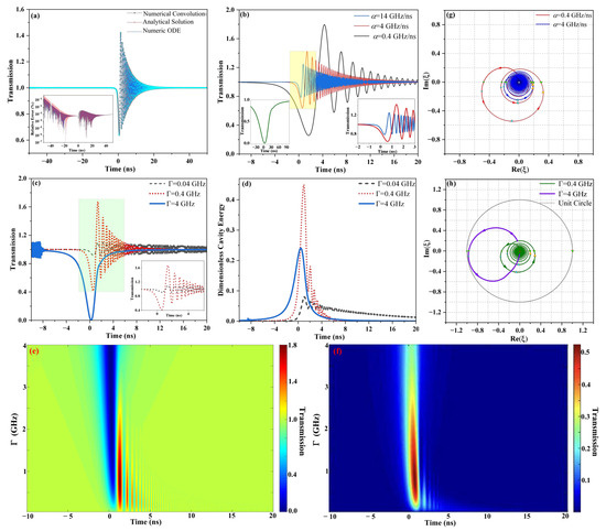
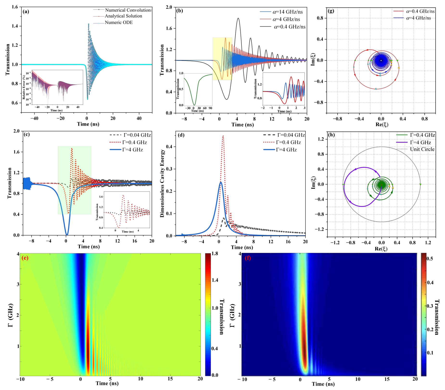
To verify the validity of the exact analytical solution given by Equation (18), we compare it with two independent numerical methods: numerically solving the ordinary differential equation (ODE) in Equation (13), and numerically integrating the convolution in Equation (17). Figure 2a shows the calculated transmission $T\left(t\right)$ versus time for a linear frequency sweep through resonance. The three curves—numerical convolution, analytical solution, and numerical ODE—are plotted together and are nearly indistinguishable. The inset displays the relative error of both the analytical solution and the numerical convolution with respect to the ODE reference. Over the entire time range of interest, the relative error remains below $0.2\%$, confirming excellent agreement among the three approaches. This validation verifies the accuracy of Equation (13), which will be used in the subsequent analysis of nonadiabatic cavity dynamics.

Figure 2. (a) Temporal evolution of the transmission under a linear frequency sweep of the input signal, calculated using the analytical expression (red stars), numerical integration of the convolution (black circles), and direct numerical solution of the dynamic equation (cyan diamonds). The inset shows the relative errors of the analytical method (navy line) and numerical convolution (red line) with respect to the numerical solution of the dynamic equation. (b) Analytically calculated temporal evolution of the transmission for sweep rates $\alpha =0.4$ GHz/ns (black line), 4 GHz/ns (red line), and 14 GHz/ns (blue line). The evolution over a longer time scale for $\alpha =0.01$ GHz/ns is shown in the left inset, while the magnified details within the shaded yellow rectangle are shown in the right inset. (c) Analytically calculated transmission and (d) dimensionless cavity energy for $\mathsf{\Gamma }=0.04$ GHz (black dashed line), $0.4$ GHz (red dotted line), and 4 GHz (blue solid line). The inset in (c) shows a magnified view of the curves within the shaded yellow-green rectangle. (e) shows the analytically calculated transmission with $\mathsf{\Gamma }$ set at $0.04$ GHz (black dashed line), $0.4$ GHz (red dotted line), and 4 GHz (blue solid line), while (f) shows the corresponding dimensionless cavity energy. (g) Calculated trajectories of the discrete–continuum ratio $\xi$ in the complex plane for $\alpha =0.4$ GHz/ns (red line) and $\alpha =4$ GHz/ns (blue line). (h) Calculated trajectories of $\xi$ for $\mathsf{\Gamma }=0.4$ GHz (green line) and $\mathsf{\Gamma }=4$ GHz (violet line). The black solid line represents the unit circle of $\xi$.

Figure 2b shows the time evolution of the transmission $T\left(t\right)$ for four different sweep rates $\alpha =0.01$, $0.4$, 4, and 14 GHz/ns, with the cavity linewidth fixed at $\mathsf{\Gamma }=0.2$ GHz. For the slowest sweep with $\alpha =0.01$ GHz/ns, the transmission closely resembles the Lorentzian lineshape typically observed under adiabatic frequency sweeping, i.e., when $\alpha$ is infinitesimally small. The slight differences are that the curve is asymmetric and the minimum does not occur exactly at the cavity resonance frequency reached at $t=0$. For the other three values of $\alpha$, the transmission deviates significantly from the Lorentzian lineshape. As the instantaneous frequency approaches the cavity resonance from below, the transmission first decreases, reaching a minimum that is blue-shifted relative to the resonance frequency. This dip results from destructive interference between the directly transmitted field and the cavity mode re-radiation. Although the cavity mode builds up near resonance, its phase is determined by the entire past history of the input via the convolution integral in Equation (17) and is therefore no longer an integer multiple of $2\pi$ as it is in the adiabatic case. Consequently, the deepest destructive interference occurs at a frequency slightly above resonance. Immediately after passing the minimum, the transmission rises rapidly, overshooting unity and forming a pronounced peak. This overshoot is followed by a train of decaying oscillations, indicating that the cavity mode continues to evolve and interfere with the input even after the instantaneous frequency has moved away from resonance. Such oscillatory behavior is a direct manifestation of the finite temporal memory inherent in the convolution solution.

Comparing the three faster sweep rates reveals a clear trade-off between the amplitude of the interference features and the frequency of the subsequent oscillations. For $\alpha =0.4$ GHz/ns, the transmission dip is the deepest and the overshoot is the largest, but the subsequent oscillations have a low frequency. For the fastest sweep with $\alpha =14$ GHz/ns, the dip and overshoot are much shallower, yet the oscillations exhibit a markedly higher frequency. The intermediate sweep rate $\alpha =4$ GHz/ns yields an intermediate behavior. This can be understood from Equation (17), where the exponential kernel limits the effective integration window to approximately $1/\mathsf{\Gamma }$. When $\alpha$ is small, the phase factor $e^{-i{\displaystyle \frac{\alpha }{2}}{(\tau -t_0)}^2}$ varies little within this window, allowing the cavity mode to build up efficiently, which produces a deep dip and a large overshoot. The slow sweep weakens the phase accumulation that governs the alternation between constructive and destructive interference, leading to low-frequency oscillations in the output. Conversely, when $\alpha$ is large, the rapid oscillation of the phase factor within the same window averages down the cavity amplitude, resulting in a shallow dip and a small overshoot. However, the rapid frequency change forces the accumulated phase to vary quickly, yielding high-frequency oscillations. This dependence on the sweep rate differs fundamentally from the traditional Landau–Zener transition of population, which typically increases with higher $\alpha$. This distinction arises because the LZSM interference of atomic polarization results from a first-order perturbation to the Bloch equations, whereas population dynamics must be calculated self-consistently. Since a direct classical counterpart to atomic population is absent in the optical resonator, population dynamics cannot be accessed in the system illustrated in Figure 1b.

Figure 2c,d show the analytically calculated transmission and dimensionless cavity energy, respectively, for three different cavity linewidths $\mathsf{\Gamma }=0.04$, $0.4$, and 4 GHz at a fixed sweep rate of $\alpha =4$ GHz/ns. The dimensionless cavity energy is defined as the intracavity energy $|\tilde{a}{\left(t\right)|}^2$ under unit input power $|{\tilde{s}}_{\mathrm{in}}{\left(t\right)|}^2=1$. For the largest linewidth of $\mathsf{\Gamma }=4$ GHz, corresponding to a short photon lifetime of ${\tau }_c=0.25$ ns, the frequency changes negligibly during the photon lifetime. Consequently, the transmission exhibits a single symmetric dip and the intracavity energy appears as a single peak, both closely resembling the adiabatic Lorentzian lineshape. When the linewidth is reduced to $\mathsf{\Gamma }=0.4$ GHz (${\tau }_c=2.5$ ns), the frequency sweeps by as much as 10 GHz within the photon lifetime, pushing the system into the nonadiabatic regime. Under these conditions, clear nonadiabatic signatures emerge, including that the transmission dip becomes asymmetric and is followed by a train of decaying oscillations, while the intracavity energy develops pronounced oscillations on the blue-detuned side of the resonance. Further reducing the linewidth to $\mathsf{\Gamma }=0.04$ GHz still yields a nonadiabatic response; however, the amplitudes of both the transmission oscillations and the intracavity energy are significantly reduced compared to the case with $\mathsf{\Gamma }=0.4$ GHz. This reduction can be understood by noting that the photon lifetime becomes so long (25 ns) that the frequency sweeps over a wide range of $\sim 100$ GHz during the convolution window. The rapidly oscillating phase factor $e^{-i{\displaystyle \frac{\alpha }{2}}{(\tau -t_0)}^2}$ averages out the convolution integral, effectively suppressing the buildup of the cavity mode.

Figure 2e,f illustrate the temporal evolution of the transmission and intracavity energy, respectively, as the cavity linewidth $\mathsf{\Gamma }$ is continuously varied from $0.04$ to 4 GHz at a fixed sweep rate of $\alpha =4$ GHz/ns. As $\mathsf{\Gamma }$ increases, the amplitude of the transient oscillations first grows, reaches a maximum, and then weakens, eventually recovering the adiabatic Lorentzian lineshape. This non-monotonic behavior reflects a trade-off between two competing factors. For very small $\mathsf{\Gamma }$, the photon lifetime is long, providing an extended memory for phase accumulation. However, the coupling between the waveguide and the cavity is proportionally weak. Consequently, the cavity mode builds up slowly and the overall excitation efficiency is low, resulting in weak transient oscillations. As $\mathsf{\Gamma }$ increases, the coupling becomes stronger, allowing the cavity mode to be excited more efficiently. Simultaneously, the photon lifetime remains sufficiently long for the nonadiabatic phase to accumulate over several oscillations, leading to pronounced transient features. If $\mathsf{\Gamma }$ becomes too large, the photon lifetime is so short that the frequency sweep does not change appreciably within the integration window. The system then exhibits a nearly steady-state response to each instantaneous frequency, recovering the adiabatic Lorentzian lineshape and suppressing transient oscillations. Thus, the most intense nonadiabatic response—characterized by the strongest transient oscillations—occurs at an intermediate linewidth, where the coupling is strong enough to efficiently excite the cavity, yet the memory time is long enough to support phase accumulation and interference. Notably, as $\mathsf{\Gamma }$ varies, the oscillation period remains nearly constant, indicating that the oscillation frequency is determined primarily by the sweep rate $\alpha$ rather than the cavity linewidth. Physically, these output oscillations arise from the rapid change in the phase difference between the directly transmitted field and the cavity-radiated field as the input frequency sweeps through resonance.

This behavior reveals a key difference between the optical resonator system and a conventional atomic population LZSM system. In the atomic case, the coupling strength G and the population relaxation rate $T_1^{-1}$ are independent parameters, meaning that a larger G increases the transition probability without directly affecting the decay of atomic coherence. In contrast, in the resonator-waveguide structure, the same parameter ${\gamma }_e$ simultaneously governs two opposing effects. On one hand, a larger ${\gamma }_e$ enhances the excitation efficiency of the cavity mode, allowing a stronger field to build up. On the other hand, it increases the total decay rate $\mathsf{\Gamma }={\gamma }_i+{\gamma }_e$, shortening the photon lifetime and thereby reducing the time available for phase accumulation and interference. Consequently, the net nonadiabatic response exhibits a non-monotonic dependence on $\mathsf{\Gamma }$.

According to the input–output relationship in Equation (12), the transmission can be generally expressed as $T\left(t\right)=|1+\sqrt{2{\gamma }_e}\tilde{a}\left(t\right)/{\tilde{s}}_{\mathrm{in}}{\left(t\right)|}^2$, allowing us to define a complex ratio $\xi \left(t\right)=\sqrt{2{\gamma }_e}\tilde{a}\left(t\right)/{\tilde{s}}_{\mathrm{in}}\left(t\right)$. In the complex plane, as $\xi$ approaches $-1$, the destructive interference dip in the transmission becomes progressively deeper, whereas as $\xi$ tends toward 1, the constructive interference peak grows increasingly higher. Figure 2g illustrates the theoretically calculated complex-plane trajectories of $\xi$ for linear frequency sweep rates $\alpha =0.4$ GHz/ns and 4 GHz/ns. In both scenarios, $\xi$ alternately passes through points with phase angles $\varphi =(2p+1)\pi$ ($p\in \mathbb{Z}$) and $\varphi =2p\pi$, marked on the trajectories by green circles and triangles, respectively. Consequently, the transmission manifests alternating dips and peaks, as depicted in Figure 2b, while the monotonic decrease in the magnitude of $\xi$ over time accurately reflects the inherently decaying nature of these oscillations. Furthermore, a comparative analysis of the two trajectories demonstrates that the higher sweep rate of $\alpha =4$ GHz/ns yields a smaller average magnitude for $\xi$, thereby resulting in the correspondingly attenuated oscillation amplitude observed in Figure 2b.

Given that the magnitudes of $\xi$ are smaller than 1 for both $\alpha =0.4$ GHz/ns and $\alpha =4$ GHz/ns, optimal conditions for destructive interference require a maximized magnitude of $\xi$ and a phase approaching $\varphi =(2p+1)\pi$. Within the half-plane of $\mathrm{Re}\left(\xi \right)<0$ in Figure 2g, the points corresponding to the maximum magnitude of $\xi$ during the initial periods are designated by cyan circles. This indicates that the nadir of the transmission dip must invariably manifest between $\varphi =(2p+1)\pi$ and the cyan circles. However, as the number of oscillation periods increases, the progressively diminishing distance between consecutive pairs of green and cyan circles suggests that, for later periods, the apex of strongest destructive interference effectively converges exactly at $\varphi =(2p+1)\pi$. Conversely, because the magnitude of $\xi$ monotonically decays with temporal evolution each time it crosses $\varphi =2p\pi$, the constructive interference peak within any given period must precede the $\varphi =2p\pi$ coordinate. Specifically, since the points immediately succeeding $\varphi =2p\pi$ that exhibit maximized imaginary and real parts are delineated by cyan and yellow triangles, respectively, the transmission peak is constrained to emerge between these two bounds. In summary, a robust criterion is established for identifying transmission extrema via the complex trajectories of $\xi$.

Figure 2h plots the theoretically calculated complex trajectories of $\xi$ for $\mathsf{\Gamma }=0.4$ GHz and 4 GHz, alongside a reference unit circle. Here, $\xi$ undergoes repeated crossings between $\varphi =(2p+1)\pi$ and $\varphi =2p\pi$ when $\mathsf{\Gamma }=0.4$ GHz, whereas it traverses $\varphi =\pi$ only once for $\mathsf{\Gamma }=4$ GHz. This fundamentally accounts for the multiple oscillations versus the isolated single-dip structure observed in Figure 2c. Furthermore, for the case with $\mathsf{\Gamma }=4$ GHz, $\mathrm{Re}\left(\xi \right)$ exhibits a negligible increase from the green to the cyan circles, while $\mathrm{Im}\left(\xi \right)$ undergoes substantial amplification. This demonstrates that the corresponding transmission dip in Figure 2c is predominantly governed by the out-of-phase interference between the continuum mode and the re-radiation emanating from the bound cavity mode.

For the experimental realization, silicon or silicon nitride microring resonators coupled to strip waveguides serve as excellent candidates. To achieve the dynamics shown in Figure 2a, the required frequency sweep range for a single resonance exceeds 10 nm, and the Q factor approaches $5\times {10}^4$ at 1550 nm; this can be experimentally realized by a compact single silicon microring resonator [59]. For the scenarios in Figure 2b–d, the sweep range is roughly 1 nm, and the maximum Q factor approaches $5\times {10}^6$ at 1550 nm. To simultaneously achieve the requisite large free spectral range and high Q factor, a compound structure comprising two cascaded microring resonators utilizing the Vernier effect can be employed [60]. Furthermore, the necessary frequency sweeps are well within the capabilities of lasers developed for swept-source optical coherence tomography. Sweep rates from $\alpha =0.01$ GHz/ns to $\alpha =4$ GHz/ns can be generated using a laser equipped with a polygon mirror scanner [61], whereas a rate of $\alpha =14$ GHz/ns is achievable with a Fourier-domain mode-locked laser [62].

3.2. Sinusoidal Frequency Modulation: Stückelberg Oscillations

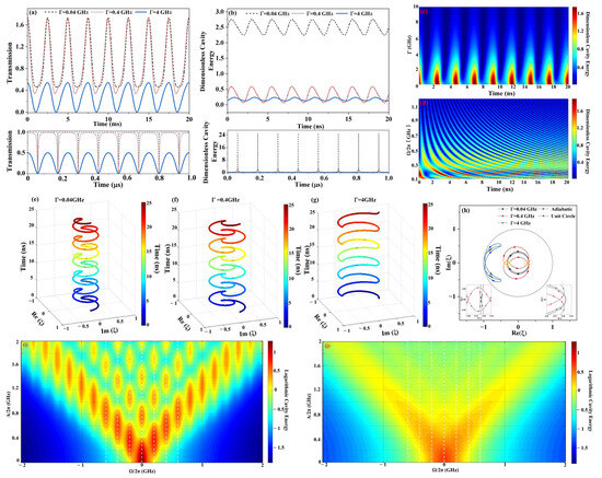
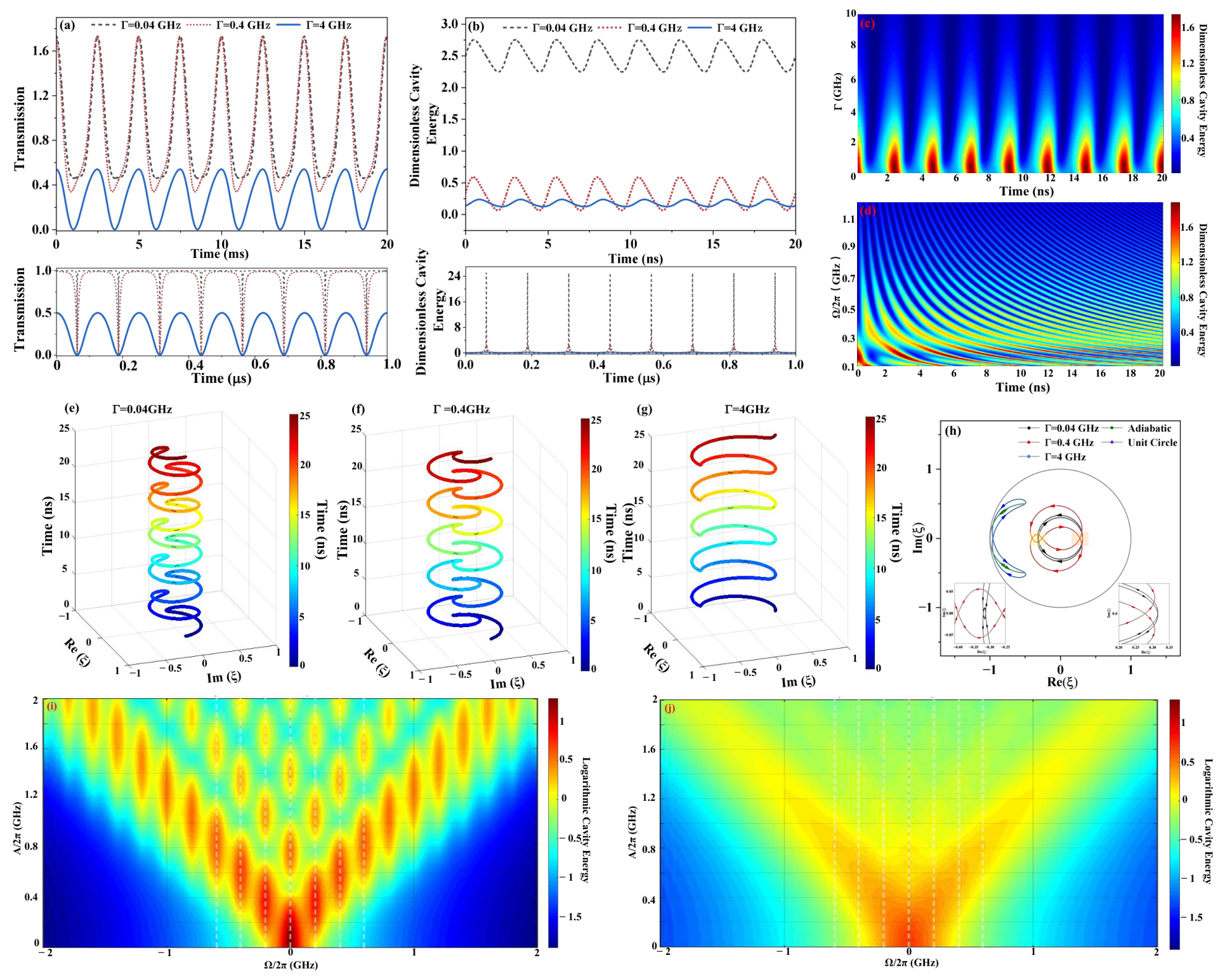
When the input signal has sinusoidal frequency modulation, the nonadiabatic response of the optical resonator can be calculated based on Equations (19) and (20). Figure 3a,b show the calculated transmission and dimensionless cavity energy, respectively, under sinusoidal frequency modulation of the input signal with a modulation depth of $A=4$ rad and a modulation frequency of $\mathsf{\Omega }/\left(2\pi \right)=0.2$ GHz. In both panels, the cavity linewidth is set to $\mathsf{\Gamma }=0.04$, $0.4$, and 4 GHz, while the intrinsic detuning $\Delta$ is set to zero. For comparison, the corresponding adiabatic responses are also plotted.

Figure 3. In (a,b), the top panels show the analytically calculated transmission and dimensionless cavity energy, respectively, under sinusoidal frequency modulation of the input signal, while the bottom panels present the corresponding adiabatic results. In the calculation of the adiabatic response, each frequency point is maintained for 50 ns. In all four panels of (a,b), the black dashed, red dotted, and blue solid lines correspond to $\mathsf{\Gamma }=0.04$ GHz, $0.4$ GHz, and 4 GHz, respectively. (c) Calculated transmission as $\mathsf{\Gamma }$ is continuously varied from $0.04$ GHz to 10 GHz. (d) Calculated transmission as the modulation frequency $\mathsf{\Omega }/2\pi$ is continuously varied from $0.1$ GHz to 2 GHz. (e–g) are the time-dependent trajectories of $\xi$ over five modulation periods for $\mathsf{\Gamma }=0.04$ GHz, $0.4$ GHz, and 4 GHz, respectively. (h) Single-period projected trajectories in the complex plane in the nonadiabatic regime for $\mathsf{\Gamma }=0.04$ GHz (black solid line), $0.4$ GHz (red solid line), and 4 GHz (blue solid line), alongside the adiabatic response (green solid line). The unit circle is indicated by violet dots. (i,j) The maximum dimensionless cavity energy as a function of A and ${\Delta }_0$ for $\mathsf{\Gamma }=0.4$ GHz and 4 GHz, respectively.

For the narrowest linewidth ($\mathsf{\Gamma }=0.04$ GHz), the cavity lifetime is much longer than the 5 ns modulation period. As the instantaneous frequency sweeps periodically across the resonance, the cavity mode undergoes a nonadiabatic excitation each time it passes through the resonance region. In the intervals far from resonance, the cavity field evolves adiabatically, accumulating a phase that depends on its entire preceding history. The interference between successive nonadiabatic excitations gives rise to Stückelberg oscillations, which are clearly visible in both the transmission and the intracavity energy. The output waveform exhibits a periodic anharmonic structure with a period equal to half of the modulation period. Over many cycles, the coherent accumulation of nonadiabatic excitations eventually balances with cavity dissipation, leading to a stable average intracavity energy, which represents the optical analog of the Landau–Zener transition of atomic polarization. When the linewidth is increased to $\mathsf{\Gamma }=0.4$ GHz, the photon lifetime decreases to about $2.5$ ns, which is still comparable to the modulation period. Coherent phase accumulation remains possible, but over a reduced number of cycles. Consequently, the average intracavity energy is lower than that for $\mathsf{\Gamma }=0.04$ GHz, and the Stückelberg oscillations become less pronounced. For $\mathsf{\Gamma }=4$ GHz, the cavity lifetime drops to approximately 250 ps, which is much shorter than the modulation period. Under this condition, nonadiabatic excitations from consecutive cycles can no longer accumulate coherently; i.e., each excitation decays before the next one occurs. The effective Landau–Zener transition probability is further reduced, and the average intracavity energy reaches its lowest value among the three cases, as shown in Figure 3b. However, the waveguide transmission in Figure 3a does not simply follow the trend of the intracavity energy. At this larger linewidth, the coupling coefficient between the resonator and the waveguide is higher, meaning that a greater portion of the cavity field participates in destructive interference with the directly transmitted continuum mode. Despite the low cavity energy, the output intensity exhibits a deep dip and a significant modulation depth. This behavior highlights the dual role of the cavity linewidth: it governs both the excitation efficiency of the cavity mode and the interference visibility via the coupling strength. The observed output transmission is determined by the competition between these two effects. In fact, at $\mathsf{\Gamma }=4$ GHz, the LZSM interference result is already very close to the adiabatic response.

In all three cases, the adiabatic response fails to capture the oscillatory structure and the asymmetric waveform. The deviation from the adiabatic limit is most pronounced for $\mathsf{\Gamma }=0.04$ GHz, where the photon lifetime is long enough to support coherent accumulation over many cycles. As $\mathsf{\Gamma }$ increases, the system gradually approaches adiabatic behavior, and at $\mathsf{\Gamma }=4$ GHz, only remnants of nonadiabatic interference remain. These observations confirm that the optical ring resonator faithfully reproduces the essential features of LZSM interference, including the coherent accumulation of nonadiabatic transitions and the resulting Stückelberg oscillations.

Figure 3c shows the temporal evolution of the transmission as the linewidth $\mathsf{\Gamma }$ is continuously varied over a wide range. In this calculation, the modulation depth and modulation frequency are set to $A=4$ rad and $\mathsf{\Omega }/\left(2\pi \right)=0.2$ GHz, respectively. When $\mathsf{\Gamma }$ is small, the Stückelberg oscillations exhibit peaks exceeding unity ($T>1$), indicating strong constructive interference between the directly transmitted field and the cavity-radiated field. As $\mathsf{\Gamma }$ increases, the peak and valley amplitudes of the output decrease progressively. For a sufficiently large $\mathsf{\Gamma }$, the frequency sweep always remains near the cavity resonance, and the output becomes very low, approaching the adiabatic response. This transition reflects the gradual loss of the coherent accumulation of nonadiabatic excitations as the photon lifetime shortens. Figure 3d presents the waveguide transmission versus time as the modulation frequency $\mathsf{\Omega }/\left(2\pi \right)$ is continuously varied from $0.1$ GHz to $1.2$ GHz with fixed $\mathsf{\Gamma }=0.4$ GHz and $A=4$ rad. As the modulation frequency increases, the oscillation frequency of the Stückelberg fringes increases accordingly, while the waveform shape changes significantly. The peak amplitude exhibits a clear overall increase accompanied by a superimposed oscillatory structure as $\mathsf{\Omega }/\left(2\pi \right)$ rises. When the modulation frequency becomes very high, the output approaches a nearly harmonic oscillation. This behavior can be understood by examining the origins of the Landau–Zener transition and Stückelberg interference. As $\mathsf{\Omega }/\left(2\pi \right)$ increases, the number of nonadiabatic passages within the photon lifetime grows, and the Landau–Zener transition probability tends to increase, leading to a higher average output. However, the relative phase between two consecutive nonadiabatic pathways also varies with $\mathsf{\Omega }/\left(2\pi \right)$, producing an oscillatory modulation of the peak amplitude. When the modulation frequency is very high, the relative phase between the two pathways becomes very small, the Stückelberg interference is significantly weakened, and the output approaches a simple harmonic oscillation.

To further explain the Stückelberg oscillations in transmission, we calculate $\xi \left(t\right)$ as in Figure 2g,h and plot the evolution of $\xi \left(t\right)$ in Figure 3e–g for $\mathsf{\Gamma }=0.04$, $0.4$, and 4 GHz, respectively. In each case, $\xi \left(t\right)$ exhibits periodic evolution, while the trajectory morphology reveals a strong dependence on the cavity linewidth $\mathsf{\Gamma }$. A clearer comparison is provided in Figure 3h, which overlays the $\xi$ trajectories over a single modulation period for all three damping rates.

When $\mathsf{\Gamma }=0.04$ GHz, the trajectory of $\xi \left(t\right)$ passes through points with $\varphi =(2p+1)\pi$ ($p\in \mathbb{Z}$) four times within one period, as shown in Figure 3h. Although the first two points are temporally far apart, the phases of nearby points on the trajectory are all close to $\varphi =(2p+1)\pi$, while the variation in the amplitude of $\xi$ remains very small. This causes the destructive interference to be distributed over a relatively large range, leading to the relatively flat bottom in the oscillation for $\mathsf{\Gamma }=0.04$ GHz shown in Figure 3a. Moreover, within one frequency sweep period, the trajectory of $\xi \left(t\right)$ during the first half of the period is the complex conjugate of the trajectory during the second half. As a result, the oscillation period of the waveguide output in Figure 3a is exactly half of the frequency sweep period. In each period, the trajectory passes twice through the points with $\varphi =2p\pi$, and the amplitude of $\xi$ varies significantly near these points, producing two sharp constructive-interference peaks in the transmission. When $\mathsf{\Gamma }$ increases to $0.4$ GHz, the amplitude of $\xi$ within a half-period varies greatly between the two $\varphi =(2p+1)\pi$ points. Therefore, only one of them forms a sharp destructive-interference dip, while the contrast of the destructive interference at the other point is lower than its surroundings, preventing the formation of a dip. Since the points with $\varphi =2p\pi$ along the trajectory have a positive $\mathrm{Re}\left(\xi \right)$, the transmission in Figure 3a still exhibits constructive-interference peaks with $T>1$. When $\mathsf{\Gamma }$ is further increased to 4 GHz, the trajectory of $\xi$ moves far away from the $\varphi =2p\pi$ points, resulting in the absence of $T>1$ peaks in the transmission shown in Figure 3a. On the other hand, within half a period, the trajectory of $\xi$ passes through the $\varphi =(2m+1)\pi$ point only once. This point lies near $\xi =-1$, forming a destructive-interference dip close to zero in the transmission. The entire trajectory of $\xi$ approaches a section of the unit circle, representing the adiabatic response under critical coupling conditions. Consequently, the transmission in Figure 3a also approaches the Lorentzian lineshape.

Figure 3i presents the time-averaged dimensionless cavity energy ${⟨\left|a\right|}^2{⟩}_t$ as a function of the modulation amplitude A and the central detuning $\Delta$ for $\mathsf{\Gamma }=0.05$ GHz. This parameter regime corresponds to the fast-passage limit of LZSM interference. The data are displayed on a logarithmic scale to reveal fine details. Distinct maxima can be observed along the lines $\Delta =m\mathsf{\Omega }$ ($m=0,\pm 1,\pm 2,\dots$), corresponding to the m-th order sideband resonances. For a given sideband order m, significant cavity excitation occurs only when A exceeds a threshold value roughly given by $A\gtrsim \left|m\right|\mathsf{\Omega }$. Only when this condition is satisfied can the frequency sweep pass through the resonance point, thereby generating a pronounced nonadiabatic response and inducing an effective Landau–Zener transition. Beyond this threshold, the cavity energy exhibits a series of oscillations superimposed on a gradual decay, appearing as alternating bright and dark bands in the logarithmic plot. The minima are located at values of A where $J_m(A/\mathsf{\Omega })=0$, indicating destructive interference for the corresponding sideband. The decaying envelope arises because the Landau–Zener transition probability decreases with increasing A, thereby reducing the energy stored in the resonator. When $\mathsf{\Gamma }$ is set to $0.2$ GHz, the LZSM interference falls into the slow-passage limit, where the cavity linewidth is comparable to the modulation frequency. In this regime, the behavior changes qualitatively, as shown in Figure 3j. Although the resonance maxima still appear near $\Delta =m\mathsf{\Omega }$, individual sidebands are no longer resolved since adjacent sidebands overlap and the spectral structure becomes blurred. Compared with Figure 3i, the oscillatory banded pattern is largely washed out, leaving only a few broad peaks distinguishable at small A. Furthermore, the amplitude of the Stückelberg oscillations is strongly suppressed. In the slow-passage limit, the cavity mode experiences almost exclusively adiabatic excitation, leading to a low Landau–Zener transition probability and suppressed Stückelberg oscillation amplitudes.

3.3. Revisiting Critical Coupling in the Nonadiabatic Regime

In waveguide-resonator coupled systems, a key concept is critical coupling, which physically corresponds to a balance between the intrinsic cavity loss rate ${\gamma }_i$ and the external coupling rate ${\gamma }_e$ (i.e., ${\gamma }_e={\gamma }_i$). Under this condition, the transmission at resonance ideally drops to zero due to perfect destructive interference between the directly transmitted field and the resonantly re-radiated field. However, whether this strict correspondence between critical coupling and zero transmission holds in the nonadiabatic regime has yet to be investigated.

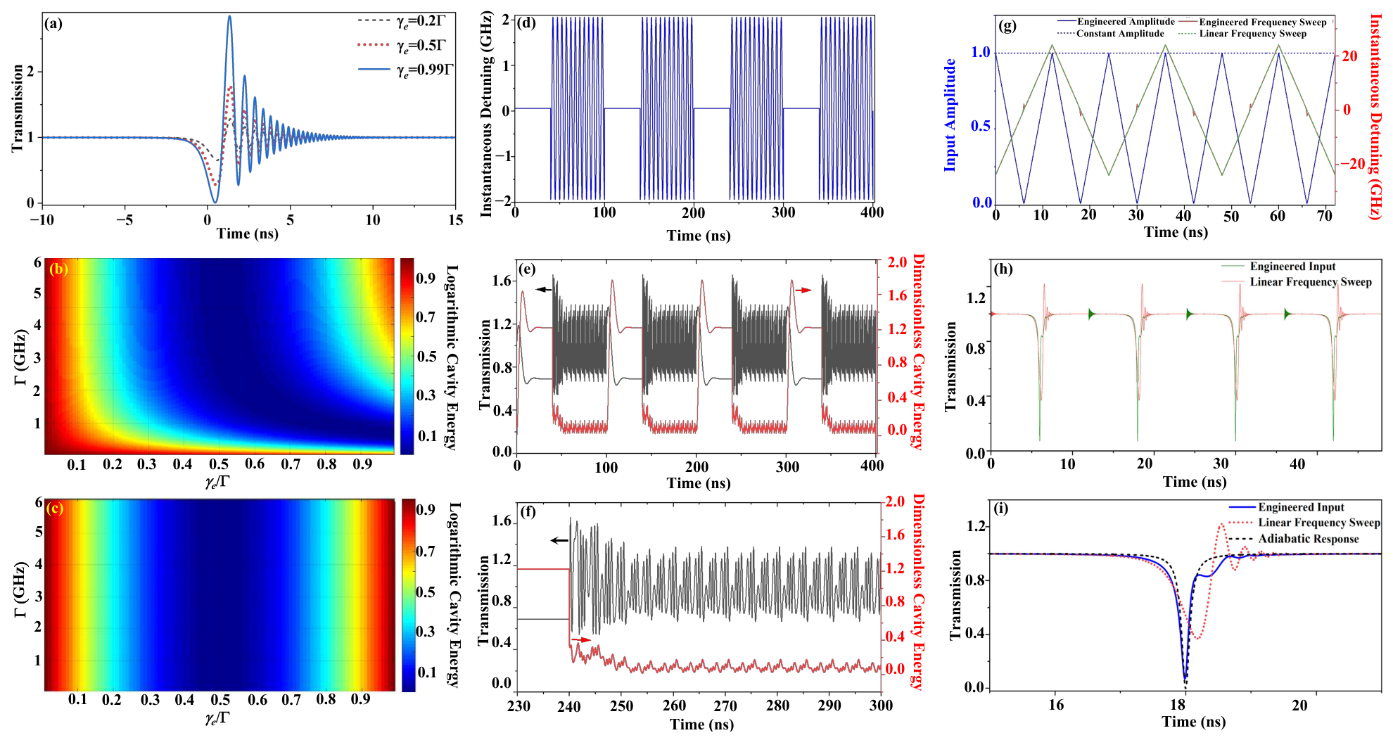
Calculated using Equation (18), the temporal evolution of the transmission is shown in Figure 4a with the total decay rate fixed at $\mathsf{\Gamma }=0.6$ GHz and the coupling coefficients set to ${\gamma }_e=0.2\mathsf{\Gamma }$, $0.5\mathsf{\Gamma }$, and $0.99\mathsf{\Gamma }$ under a linear frequency sweep. These three values of ${\gamma }_e$ correspond to the under-coupled, critically coupled, and over-coupled conditions, respectively. In the adiabatic limit, they are expected to produce narrow and shallow, moderately narrow and deep, and broad and shallow transmission dips, respectively. Counterintuitively, in the nonadiabatic regime shown in Figure 4a, the over-coupled case yields the deepest transmission dip. For a fixed $\mathsf{\Gamma }$, increasing the external coupling rate ${\gamma }_e$ enhances the energy exchange between the resonator and the waveguide, thereby promoting cavity excitation even when the input frequency is chirped. From the perspective of the Landau–Zener transition formula [2], the nonadiabatic transition probability increases with the coupling strength for a fixed total linewidth.

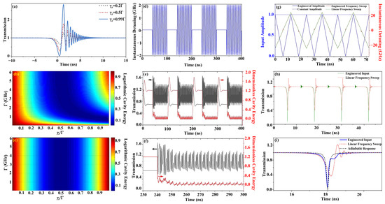
Figure 4. (a) Theoretically calculated temporal evolution of the transmission for ${\gamma }_e=0.2\mathsf{\Gamma }$ (black dashed line), ${\gamma }_e=0.5\mathsf{\Gamma }$ (red dotted line), and ${\gamma }_e=0.99\mathsf{\Gamma }$ (blue solid line). (b,c) Theoretically calculated dependence of the nonadiabatic and adiabatic transmission on ${\gamma }_e/\mathsf{\Gamma }$ and $\mathsf{\Gamma }$, respectively. (d) Instantaneous detuning of the input signal, featuring alternating intervals of constant frequency and sinusoidal frequency modulation. (e) Temporal evolution of the transmission (black line) and cavity mode energy (red line) for the input signal shown in (d). (f) Magnified view of the dynamics in (e) for the time window between 230 ns and 300 ns. In (e,f), the black and red arrows indicate that the black and red lines correspond to the left and right vertical axes, respectively. (g) Amplitudes and instantaneous detunings of the engineered amplitude-and-frequency-modulated signal and the standard linearly frequency-swept signal. The blue solid and red solid lines represent the amplitude and instantaneous detuning of the engineered signal, respectively, while the black dotted and green dotted lines represent the corresponding quantities for the linearly swept signal. (h) Temporal evolution of the transmission for the engineered signal (green line) and the linearly swept signal (red line). (i) Magnified view of the transmission evolution within a single period. The blue solid, red dotted, and black dashed lines correspond to the engineered signal, the linearly swept signal, and the adiabatic response, respectively.

Figure 4b illustrates the depth of the first transmission dip under continuous variations of $\mathsf{\Gamma }$ and the ratio ${\gamma }_e/\mathsf{\Gamma }$ when the input frequency is linearly swept, while Figure 4c shows the corresponding adiabatic results. As observed in Figure 4b, when $\mathsf{\Gamma }$ is relatively small, increasing ${\gamma }_e/\mathsf{\Gamma }$ significantly enhances the depth of the transmission dip. This enhancement occurs because a larger ${\gamma }_e/\mathsf{\Gamma }$ markedly improves the nonadiabatic excitation efficiency of the cavity mode, corresponding to a higher Landau–Zener transition probability. Conversely, when $\mathsf{\Gamma }$ is large, the optimal condition for the deepest transmission dip gradually converges to ${\gamma }_e/\mathsf{\Gamma }=1/2$. This is attributed to the excessively short photon lifetime under these conditions, which renders the nonadiabatic phase accumulation inefficient. Consequently, the nonadiabatic response in Figure 4b approaches the adiabatic response shown in Figure 4c. This underlying behavior reflects a trade-off mechanism between the absolute coupling rate and coherent phase accumulation, similar to what is observed in Figure 2e.

In a potential experimental implementation using waveguide-coupled microring resonators, the external coupling rate ${\gamma }_e$ can be precisely controlled by adjusting the coupling gap between the waveguide and the resonator [63].Independent tuning of the intrinsic loss rate ${\gamma }_i$ can be achieved by introducing an auxiliary coupling waveguide or by inserting a movable near-field tip into the evanescent field of the resonators to introduce controlled scattering loss [64].

3.4. LZSM Interference for Complex and Engineered Modulation

Based on the theory presented in Section 2, the LZSM interference originates from the non-negligible memory effect of the cavity mode with respect to the input field. Consequently, optical fields with distinct time–frequency distributions can induce qualitatively different LZSM interference patterns. In contrast to the previously studied linear frequency chirp starting from negative infinity and the continuous sinusoidal frequency modulation, a pulsed frequency-modulated field can be designed to generate more complex interference fringes. In this scheme, the field amplitude remains constant, while its frequency switches periodically between a fixed detuning ${\Delta }_0$ and a modulated detuning ${\Delta }_0+A\cos \left(\mathsf{\Omega }t\right)$. Figure 4d shows the time evolution of the instantaneous detuning for this engineered input field.

In each modulation segment $t\in [t_1,t_2]$, Equation (13) has the solution

$$\tilde{a}\left(t\right)=\left[\tilde{a}\left(t_1\right)-{\displaystyle \frac{\sqrt{2{\gamma }_e}}{i{\Delta }_0-\mathsf{\Gamma }}}\right]e^{(i{\Delta }_0-\mathsf{\Gamma })(t-t_1)}-{\displaystyle \frac{\sqrt{2{\gamma }_e}}{i{\Delta }_0-\mathsf{\Gamma }}}$$

(21)

for the fixed detuning segment, and

$$\begin{array}{cc}\hfill \tilde{a}\left(t\right)=& \left[\tilde{a}\left(t_1\right)-{\displaystyle \sum _{m=-\infty }^{\infty }}{\displaystyle \frac{\sqrt{2{\gamma }_e}{J}_m(A/\mathsf{\Omega })}{i({\Delta }_0+mA/\mathsf{\Omega })-\mathsf{\Gamma }}}\right]e^{-(i{\Delta }_0+\mathsf{\Gamma })(t-t_1)}\hfill \\ & -{\displaystyle \sum _{m=-\infty }^{\infty }}{\displaystyle \frac{\sqrt{2{\gamma }_e}{J}_m(A/\mathsf{\Omega })}{i({\Delta }_0+mA/\mathsf{\Omega })-\mathsf{\Gamma }}}{e}^{im\mathsf{\Omega }(t-t_1)},\hfill \end{array}$$

(22)

for the sinusoidal detuning modulation. On the right-hand side of both Equations (21) and (22), the first and second terms represent the transient and steady-state responses, respectively. Using these expressions, we sequentially calculate the nonadiabatic response for each modulation segment. The resulting temporal evolution of the transmission and the intracavity energy are shown in Figure 4e. For both the fixed and sinusoidally modulated detuning segments, a transient response is observed before the system settles into a steady state. This transient response arises from the abrupt frequency switching, which effectively acts as a rapid frequency sweep and thus drives a distinct Landau–Zener transition. Within the fixed detuning segments, cavity dissipation forces the cavity excitation induced by the Landau–Zener transition to gradually relax toward a steady-state value determined by the adiabatic response under a constant detuning. In contrast, within the sinusoidally modulated segments, the sudden frequency jump and the subsequent continuous frequency modulation are superimposed via the cavity memory effect, giving rise to pronounced transient dynamics at the beginning of each segment. Figure 4f displays a magnified view of a single modulated segment extracted from Figure 4e. Although the cavity mode amplitude does not exhibit a drastic change, its phase varies rapidly, leading to significant oscillations in the transmission. These oscillations gradually damp out and evolve into steady-state Stückelberg oscillations. The parameters chosen for this calculation are $\mathsf{\Gamma }=0.04$ GHz, $A/\left(2\pi \right)=4$ GHz, $\mathsf{\Omega }/\left(2\pi \right)=0.2$ GHz, and ${\Delta }_0=0.06$ GHz. Under these conditions, the higher-order harmonic components of the Stückelberg oscillation are clearly resolved, and multiple oscillations occur within a single modulation period.

The results shown in Figure 4e,f also reveal that adiabaticity and the steady state are two distinct concepts. The Stückelberg oscillation can indeed reach a steady state, even though its origin involves nonadiabatic phase accumulation. In other words, the steady-state interference pattern is built upon phase differences acquired during nonadiabatic passages through resonance, despite the asymptotic dynamics appearing periodic and stationary.

It can be inferred from Equation (17) that the LZSM interference pattern is jointly determined by the intrinsic response function of the waveguide-cavity system and the temporal evolution of the amplitude and phase of the input field. Consequently, it becomes possible to engineer the input signal via inverse design to customize the LZSM interference fringes.

As shown in Figure 2b, the LZSM interference fringes obtained with purely linearly frequency-swept signals deviate significantly from the Lorentzian lineshape characteristic of the adiabatic response. Based on Equation (14), an inverse design model (see the Supplementary Materials for details) is established to engineer both the amplitude envelope and the frequency chirp profile of the input field. This approach enables the LZSM transmission dip to be restored to the adiabatic response lineshape. Figure 4g presents the amplitude profile and instantaneous detuning of the engineered signal. The engineered input signal exhibits a deliberately shaped amplitude and frequency trajectory designed to compensate for the nonadiabatic memory effects inherent in the cavity response. Figure 4h shows the transmission of the engineered input signal, obtained by numerically solving Equation (13), alongside the numerically solved response for a signal with a purely periodic linear frequency sweep for comparison. Whereas the pure linear frequency sweep yields a characteristic pattern of decaying oscillatory fringes, the engineered signal produces a clean interference pattern with negligible oscillations and no overshoot. A direct comparison of the single-period transmission profiles is shown in Figure 4i, where the transmission dip produced by the engineered input closely approximates the Lorentzian lineshape of the ideal adiabatic response, while the unshaped signal exhibits substantial deviation. It is worth emphasizing that our inverse design model is currently formulated for a single period of the frequency sweep. The residual discrepancy between the engineered transmission and the ideal Lorentzian lineshape arises from Landau–Zener transitions that occurred during the preceding temporal history and persist into the steady-state response. This limitation can be overcome by extending the inverse design framework to account for multiple periods, thereby compensating for the cumulative effects of repeated nonadiabatic transitions across successive frequency sweeps.

4. Conclusions

In this work, we have explored whether Landau–Zener–Stückelberg–Majorana (LZSM) interference, traditionally characterized through population dynamics, can also emerge in atomic polarization dynamics and be investigated using an all-optical platform. By exploiting the formal correspondence between optical resonators and weakly driven TLS, we established an atomic polarization-based framework for studying LZSM interference in optical ring resonators using temporal coupled-mode theory. Exact analytical solutions have been derived for two representative driving schemes. For linear frequency sweep and sinusoidal frequency modulation of the input signal, the cavity fields are expressed in terms of complex error functions and Bessel series, respectively, while a bound-to-continuum complex ratio is defined to explain the interference pattern in the transmission.

The theoretical results revealed several key features of the nonadiabatic dynamics. The transmission for linear frequency sweep exhibits a train of decaying oscillations following the main dip, which is analogous to Landau–Zener transition and directly reflects the finite temporal memory of the cavity response. The oscillation period is determined by the sweep rate, while the amplitude depends non-monotonically on the cavity linewidth due to the competition between excitation and decay of the cavity mode. For sinusoidal modulation, we demonstrated that the cavity energy and transmission exhibit Stückelberg oscillations with a period half that of the modulation frequency. The complex-plane trajectory of the bound-to-continuum ratio provides a unified criterion to find the dips and peaks in the Stückelberg oscillations of transmission. The fast-passage and slow-passage limits of LZSM interference are clearly distinguished by the resolution of sideband resonances in the time-averaged intracavity energy.

The limitations of the critical coupling concept in the nonadiabatic regime is discussed, and the results show that the over-coupled condition yields the deepest transmission dip, contrary to the adiabatic expectation that critical coupling produces perfect destructive interference. Finally, we demonstrated an inverse-design approach that engineers both the amplitude and frequency modulation of the input field to tailor the LZSM interference pattern. Utilizing this approach, we have successfully shaped the nonadiabatic transmission to approximate the adiabatic Lorentzian lineshape when the nonadiabatic memory effects are effectively compensated.

While this study is restricted to the weak-excitation regime, the proposed framework suggests a natural extension toward nonlinear LSZM phenomena [10,65,66]. In atomic systems, nonlinear effects may arise from atom–atom interactions or higher-order optical responses beyond the weak-excitation approximation, where the evolution of atomic polarization is governed by nonlinear dynamical equations. Although the analytical convolution framework developed here is no longer directly applicable, the atomic polarization remains the central observable and the resulting nonlinear dynamics are expected to exhibit substantially richer nonadiabatic phenomena. Correspondingly, optical resonators incorporating Kerr or saturable nonlinearities [52,67] provide a natural classical platform for simulating such nonlinear dynamics. The nonlinear phase accumulated during successive Landau–Zener transitions may give rise to modified interference conditions, leading to phenomena such as deformation and shifts of Stückelberg interference fringes [10,66].

References

- Shevchenko, S.N.; Ashhab, S.; Nori, F. Landau–Zener–Stückelberg interferometry. Phys. Rep. 2010, 492, 1–30. [Google Scholar] [CrossRef]
- Ivakhnenko, V.; Shevchenko, S.N.; Nori, F. Nonadiabatic Landau–Zener–Stückelberg–Majorana transitions, dynamics, and interference. Phys. Rep. 2023, 995, 1–89. [Google Scholar] [CrossRef]
- Di Giacomo, F.; Nikitin, E.E. The Majorana formula and the Landau–Zener–Stückelberg treatment of the avoided crossing problem. Phys.-Usp. 2005, 48, 515–517. [Google Scholar] [CrossRef]
- Damski, B. The simplest quantum model supporting the Kibble-Zurek mechanism of topological defect production: Landau-Zener transitions from a new perspective. Phys. Rev. Lett. 2005, 95, 035701. [Google Scholar] [CrossRef] [PubMed]
- Shytov, A.V. Landau-Zener transitions in a multilevel system: An exact result. Phys. Rev. A 2004, 70, 052708. [Google Scholar] [CrossRef]
- Ao, P.; Rammer, J. Influence of dissipation on the Landau-Zener transition. Phys. Rev. Lett. 1989, 62, 3004. [Google Scholar] [CrossRef] [PubMed]
- Huang, Z.; Zhao, Y. Dynamics of dissipative Landau-Zener transitions. Phys. Rev. A 2018, 97, 013803. [Google Scholar] [CrossRef]
- Avishai, Y.; Band, Y.B. Landau-Zener problem with decay and dephasing. Phys. Rev. A 2014, 90, 032116. [Google Scholar] [CrossRef]
- Grifoni, M.; Hänggi, P. Driven quantum tunneling. Phys. Rep. 1998, 304, 229–354. [Google Scholar] [CrossRef]
- Li, S.-C.; Fu, L.-B.; Liu, J. Nonlinear Landau-Zener-Stückelberg-Majorana interferometry. Phys. Rev. A 2018, 98, 013601. [Google Scholar] [CrossRef]
- Oliver, J.W.D.; Yu, Y.; Lee, J.C.; Berggren, K.K.; Levitov, L.S.; Orlando, T.P. Mach-Zehnder interferometry in a strongly driven superconducting qubit. Science 2005, 310, 1653–1657. [Google Scholar] [CrossRef] [PubMed]
- Berns, D.M.; Rudner, M.S.; Valenzuela, S.O.; Berggren, K.K.; Oliver, W.D.; Levitov, L.S.; Orlando, T.P. Amplitude spectroscopy of a solid-state artificial atom. Nature 2008, 455, 51–57. [Google Scholar] [CrossRef] [PubMed]
- Sun, G.; Wen, X.; Wang, Y.; Cong, S.; Chen, J.; Kang, L.; Xu, W.; Yu, Y.; Han, S.; Wu, P. Population inversion induced by Landau–Zener transition in a strongly driven rf superconducting quantum interference device. Appl. Phys. Lett. 2009, 94, 102502. [Google Scholar] [CrossRef]
- Xiang, Z.-L.; Ashhab, S.; You, J.Q.; Nori, F. Hybrid quantum circuits: Superconducting circuits interacting with other quantum systems. Rev. Mod. Phys. 2013, 85, 623–653. [Google Scholar] [CrossRef]
- Mark, M.; Kraemer, T.; Waldburger, P.; Herbig, J.; Chin, C.; Nägerl, H.-C.; Grimm, R. “Stückelberg interferometry” with ultracold molecules. Phys. Rev. Lett. 2007, 99, 113201. [Google Scholar] [CrossRef] [PubMed]
- Kling, S.; Salger, T.; Grossert, C.; Weitz, M. Atomic Bloch-Zener oscillations and Stückelberg interferometry in optical lattices. Phys. Rev. Lett. 2010, 105, 215301. [Google Scholar] [CrossRef] [PubMed]
- Liang, S.; Li, Z.-C.; Zhang, W.; Zhou, L.; Lan, Z. Stückelberg interferometry using spin-orbit-coupled cold atoms in an optical lattice. Phys. Rev. A 2020, 102, 033332. [Google Scholar] [CrossRef]
- Liu, W.-X.; Wang, T.; Zhang, X.-F.; Li, W.-D. Time-domain Landau-Zener-Stückelberg-Majorana interference in an optical lattice clock. Phys. Rev. A 2021, 104, 053318. [Google Scholar] [CrossRef]
- Tan, W.; Liu, W.-X.; Chen, Y.-X.; Zhou, C.-H.; Zhao, G.-D.; Chang, H.; Dai, J.; Wang, T. Realization of Landau-Zener Rabi oscillations on an optical lattice clock. Phys. Rev. A 2025, 111, 033102. [Google Scholar] [CrossRef]
- Saquet, N.; Cournol, A.; Beugnon, J.; Robert, J.; Pillet, P.; Vanhaecke, N. Landau-Zener transitions in frozen pairs of Rydberg atoms. Phys. Rev. Lett. 2010, 104, 133003. [Google Scholar] [CrossRef] [PubMed]
- Petta, J.R.; Lu, H.; Gossard, A.C. A coherent beam splitter for electronic spin states. Science 2010, 327, 669–672. [Google Scholar] [CrossRef] [PubMed]
- Cao, G.; Li, H.-O.; Tu, T.; Wang, L.; Zhou, C.; Xiao, M.; Guo, G.-C.; Jiang, H.-W.; Guo, G.-P. Ultrafast universal quantum control of a quantum-dot charge qubit using Landau–Zener–Stückelberg interference. Nat. Commun. 2013, 4, 1401. [Google Scholar] [CrossRef] [PubMed]
- Stehlik, J.; Dovzhenko, Y.; Petta, J.R.; Johansson, J.R.; Nori, F.; Lu, H.; Gossard, A.C. Landau-Zener-Stückelberg interferometry of a single electron charge qubit. Phys. Rev. B 2012, 86, 121303. [Google Scholar] [CrossRef]
- Forster, F.; Petersen, G.; Manus, S.; Hänggi, P.; Schuh, D.; Wegscheider, W.; Kohler, S.; Ludwig, S. Characterization of qubit dephasing by Landau-Zener-Stückelberg-Majorana interferometry. Phys. Rev. Lett. 2014, 112, 116803. [Google Scholar] [CrossRef] [PubMed]
- Ward, D.R.; Kim, D.; Savage, D.E.; Lagally, M.G.; Foote, R.H.; Friesen, M.; Coppersmith, S.N.; Eriksson, M.A. State-conditional coherent charge qubit oscillations in a Si/SiGe quadruple quantum dot. npj Quantum Inf. 2016, 2, 16032. [Google Scholar] [CrossRef]
- Huang, P.; Zhou, J.; Fang, F.; Kong, X.; Xu, X.; Ju, C.; Du, J. Landau-Zener-Stückelberg interferometry of a single electronic spin in a noisy environment. Phys. Rev. X 2011, 1, 011003. [Google Scholar] [CrossRef]
- Zhou, J.; Huang, P.; Zhang, Q.; Wang, Z.; Tan, T.; Xu, X.; Shi, F.; Rong, X.; Ashhab, S.; Du, J. Observation of Time-Domain Rabi Oscillations in the Landau-Zener Regime with a Single Electronic Spin. Phys. Rev. Lett. 2014, 112, 010503. [Google Scholar] [CrossRef] [PubMed]
- Ajoy, A.; Liu, K.; Nazaryan, R.; Lv, X.; Zangara, P.R.; Safvati, B.; Wang, G.; Arnold, D.; Li, G.; Lin, A.; et al. Orientation-independent room temperature optical 13C hyperpolarization in powdered diamond. Sci. Adv. 2018, 4, eaar5492. [Google Scholar] [CrossRef] [PubMed]
- Miao, K.C.; Bourassa, A.; Anderson, C.P.; Whiteley, S.J.; Crook, A.L.; Bayliss, S.L.; Wolfowicz, G.; Thiering, G.; Udvarhelyi, P.; Ivády, V.; et al. Electrically driven optical interferometry with spins in silicon carbide. Sci. Adv. 2019, 5, eaay0527. [Google Scholar] [CrossRef] [PubMed]
- Guo, A.-L.; Tu, T.; Zhu, L.-T.; Li, C.-F.; Guo, G.-C. Geometric Landau-Zener-Stückelberg-Majorana interferometry for hybrid spin registers. Phys. Rev. A 2022, 106, 032411. [Google Scholar] [CrossRef]
- Xia, S.; Danieli, C.; Zhang, Y.; Zhao, X.; Lu, H.; Tang, L.; Li, D.; Song, D.; Chen, Z. Higher-order exceptional point and Landau–Zener Bloch oscillations in driven non-Hermitian photonic Lieb lattices. APL Photonics 2021, 6, 126102. [Google Scholar] [CrossRef]
- Wang, S.; Qin, C.; Zhao, L.; Ye, H.; Longhi, S.; Lu, P.; Wang, B. Photonic Floquet Landau-Zener tunneling and temporal beam splitters. Sci. Adv. 2023, 9, eadh0415. [Google Scholar] [CrossRef] [PubMed]
- Hu, S.; Li, S.; Hu, M.; Lei, Z. Symmetry-protected Landau-Zener-Stückelberg-Majorana interference and nonadiabatic topological transport of edge states. Phys. Rev. A 2025, 111, 052414. [Google Scholar] [CrossRef]
- Heinrich, G.; Harris, J.G.E.; Marquardt, F. Photon shuttle: Landau-Zener-Stückelberg dynamics in an optomechanical system. Phys. Rev. A 2010, 81, 011801. [Google Scholar] [CrossRef]
- Wu, H.; Heinrich, G.; Marquardt, F. The effect of Landau–Zener dynamics on phonon lasing. New J. Phys. 2013, 15, 123022. [Google Scholar] [CrossRef]
- Fleischhauer, M.; Lukin, M.D. Dark-state polaritons in electromagnetically induced transparency. Phys. Rev. Lett. 2000, 84, 5094. [Google Scholar] [CrossRef] [PubMed]
- Liu, X.-J.; Jing, H.; Ge, M.-L. Solitons formed by dark-state polaritons in an electromagnetic induced transparency. Phys. Rev. A 2004, 70, 055802. [Google Scholar] [CrossRef]
- Fleischhauer, M.; Imamoglu, A.; Marangos, J.P. Electromagnetically induced transparency: Optics in coherent media. Rev. Mod. Phys. 2005, 77, 633–673. [Google Scholar] [CrossRef]
- Zhang, S.; Hu, Y.; Lin, G.; Niu, Y.; Xia, K.; Gong, J.; Gong, S. Thermal-motion-induced non-reciprocal quantum optical system. Nat. Photonics 2018, 12, 744–748. [Google Scholar] [CrossRef]
- Guo, J.; Feng, X.; Yang, P.; Yu, Z.; Chen, L.Q.; Yuan, C.-H.; Zhang, W. High-performance Raman quantum memory with optimal control in room temperature atoms. Nat. Commun. 2019, 10, 148. [Google Scholar] [CrossRef] [PubMed]
- Chen, Y.; Wang, C.; Jiang, Z.; Zhang, W.; Shen, Z.; Gao, H.; Li, F. Angular dependence of spatial frequency modulation in diffusion media. Phys. Rev. A 2022, 106, 013704. [Google Scholar] [CrossRef]
- Li, J.-F.; Wang, Y.-F.; Huang, P.-S.; Su, K.-Y.; Peng, Y.-Q.; Zhang, S.; Yan, H.; Zhu, S.-L. Nonreciprocity in cold atoms based on electromagnetically induced transparency. Phys. Rev. Appl. 2023, 20, 014027. [Google Scholar] [CrossRef]
- Zhang, H.-B.; Tang, Y.; Liu, Y.-C. Nuclear spin induced transparency. Phys. Rev. Res. 2025, 7, L012069. [Google Scholar] [CrossRef]
- Xiao, M.; Li, Y.-Q.; Jin, S.-Z.; Gea-Banacloche, J. Measurement of dispersive properties of electromagnetically induced transparency in rubidium atoms. Phys. Rev. Lett. 1995, 74, 666. [Google Scholar] [CrossRef] [PubMed]
- Wang, H.; Goorskey, D.; Xiao, M. Enhanced Kerr nonlinearity via atomic coherence in a three-level atomic system. Phys. Rev. Lett. 2001, 87, 073601. [Google Scholar] [CrossRef] [PubMed]
- Chen, B.; Qiu, S.; Guo, J.; Chen, L.Q.; Ou, Z.Y.; Zhang, W. Atom-light hybrid interferometer. Phys. Rev. A 2015, 91, 023823. [Google Scholar]
- Sherkunov, Y.; Whittaker, D.M.; Fal’ko, V. Superradiance and subradiance in a photonic waveguide. Phys. Rev. A 2016, 93, 023843. [Google Scholar] [CrossRef]
- Xu, Q.; Sandhu, S.; Povinelli, M.L.; Shakya, J.; Fan, S.; Lipson, M. Experimental Realization of an On-Chip All-Optical Analogue to Electromagnetically Induced Transparency. Phys. Rev. Lett. 2006, 96, 123901. [Google Scholar] [CrossRef] [PubMed]
- Liu, Y.-C.; Xiao, Y.-F.; Luan, X.; Wong, C.W. Optomechanically-induced-transparency cooling of massive mechanical resonators to the quantum ground state. Sci. China Phys. Mech. Astron. 2015, 58, 050301. [Google Scholar] [CrossRef]
- Guo, S.-T.; Zhang, Y.-H.; Wu, L.-L.; Ye, M.-Y.; Lin, X.-M. Transition between coupled-resonator-induced transparency and absorption. Phys. Rev. A 2021, 103, 033510. [Google Scholar] [CrossRef]
- Haus, H.A.; Huang, W. Coupled-mode theory. Proc. IEEE 1991, 79, 1505–1518. [Google Scholar] [CrossRef]
- Cao, Q.-T.; Wang, H.; Dong, C.-H.; Jing, H.; Liu, R.-S.; Chen, X.; Ge, L.; Gong, Q.; Xiao, Y.-F. Experimental demonstration of spontaneous chirality in a nonlinear microresonator. Phys. Rev. Lett. 2017, 118, 033901. [Google Scholar] [CrossRef] [PubMed]
- Zhao, Z.; Guo, C.; Fan, S. Connection of temporal coupled-mode-theory formalisms for a resonant optical system and its time-reversal conjugate. Phys. Rev. A 2019, 99, 033839. [Google Scholar] [CrossRef]
- Ioannidis, Z.K.; Radmore, P.M.; Giles, I.P. Dynamic response of an all-fiber ring resonator. Opt. Lett. 1988, 13, 422–424. [Google Scholar] [CrossRef] [PubMed]
- Seraji, F.E. Dynamic response of a fiber-optic ring resonator: Analysis with influences of light-source parameters. Prog. Quantum Electron. 2009, 33, 110–125. [Google Scholar] [CrossRef]
- DeVoe, R.G.; Brewer, R.G. Experimental test of the optical Bloch equations for solids. Phys. Rev. Lett. 1983, 50, 1269–1272. [Google Scholar] [CrossRef]
- Zhu, X.; Xiong, X.; Zhu, Z.; Liu, W.; Cao, Q.-T.; Xiao, Y.-F. Engineering Dispersive-Dissipative Modal Coupling in Hybrid Optical Microresonators. Phys. Rev. Lett. 2024, 132, 223801. [Google Scholar] [CrossRef] [PubMed]
- Biasi, S.; Guillemé, P.; Volpini, A.; Fontana, G.; Pavesi, L. Time response of a microring resonator to a rectangular pulse in different coupling regimes. J. Light. Technol. 2019, 37, 5091–5099. [Google Scholar] [CrossRef]
- Xiao, S.; Khan, M.H.; Shen, H.; Qi, M. Compact silicon microring resonators with ultra-low propagation loss in the C band. Opt. Express 2007, 15, 14467–14475. [Google Scholar] [CrossRef] [PubMed]
- Boeck, R.; Jaeger, N.A.F.; Rouger, N.; Chrostowski, L. Series-coupled silicon racetrack resonators and the Vernier effect: Theory and measurement. Opt. Express 2010, 18, 25151–25157. [Google Scholar] [CrossRef] [PubMed]
- Mao, Y.; Chang, S.; Murdock, E.; Flueraru, C. Simultaneous dual-wavelength-band common-path swept-source optical coherence tomography with single polygon mirror scanner. Opt. Lett. 2011, 36, 1990–1992. [Google Scholar] [CrossRef] [PubMed]
- Wieser, W.; Biedermann, B.R.; Klein, T.; Eigenwillig, C.M.; Huber, R. Multi-Megahertz OCT: High quality 3D imaging at 20 million A-scans and 4.5 GVoxels per second. Opt. Express 2010, 18, 14685–14704. [Google Scholar] [CrossRef] [PubMed]
- Tseng, C.-W.; Tsai, C.-W.; Lin, K.-C.; Lee, M.-C.; Chen, Y.-J. Study of coupling loss on strongly-coupled, ultra compact microring resonators. Opt. Express 2013, 21, 7250–7257. [Google Scholar] [CrossRef] [PubMed]
- Peng, B.; Özdemir, Ş.K.; Rotter, S.; Yilmaz, H.; Liertzer, M.; Monifi, F.; Bender, C.M.; Nori, F.; Yang, L. Loss-induced suppression and revival of lasing. Science 2014, 346, 328–332. [Google Scholar] [CrossRef] [PubMed]
- Dou, F.Q.; Fu, L.B.; Liu, J. High-fidelity fast quantum driving in nonlinear systems. Phys. Rev. A 2014, 89, 012123. [Google Scholar] [CrossRef]
- Wang, X.; Liu, H.D.; Fu, L.B. Nonlinear non-Hermitian Landau–Zener–Stückelberg–Majorana interferometry. New J. Phys. 2023, 25, 043032. [Google Scholar] [CrossRef]
- Hassan, A.U.; Hodaei, H.; Miri, M.-A.; Khajavikhan, M.; Christodoulides, D.N. Nonlinear reversal of the PT-symmetric phase transition in a system of coupled semiconductor microring resonators. Phys. Rev. A 2015, 92, 063807. [Google Scholar] [CrossRef]
Disclaimer/Publisher’s Note: The statements, opinions and data contained in all publications are solely those of the individual author(s) and contributor(s) and not of MDPI and/or the editor(s). MDPI and/or the editor(s) disclaim responsibility for any injury to people or property resulting from any ideas, methods, instructions or products referred to in the content. |
© 2026 by the authors. Licensee MDPI, Basel, Switzerland. This article is an open access article distributed under the terms and conditions of the Creative Commons Attribution (CC BY) license.