


Abstract
Visible light positioning (VLP) based on received signal strength (RSS) offers a low-cost solution for indoor localization, being easily implemented in a warehouse based on existing infrastructure. However, RSS-based VLP remains challenging in 3D and yields subpar performance compared to 2D due to the larger localization space, as well as the presence of dark spots where many LEDs are not bright enough. This limits the practical use cases of RSS-based VLP in industrial applications. We study the performance of RSS-based VLP on a 3D simulated environment by training various machine learning models, including Gaussian processes and Kolmogorov–Arnold networks on different representations of RSS data. Our findings show that the use of Gaussian processes for predicting distances to LEDs coupled with a logarithmic transformation and multilateration leads to both high-accuracy and high-precision predictions under thermal noise (p95 localization error of 10 cm under 50 dB SNR). With this technique, RSS-based VLP reaches levels of accuracy in our simulated 3D environment that are comparable to those reported for 2D applications, supporting the extension of RSS-based VLP to height-varying industrial use cases.
1. Introduction
The inability of global localization systems such as GPS to provide accurate position estimates indoors creates a demand for dedicated indoor localization techniques [1], which is exacerbated by the advent of automated vehicles in warehouses. Among the variety of techniques used in indoor positioning, visible light positioning (VLP) stands out as a good option due to its high precision and lack of need for expensive equipment or extensive computing power. Moreover, VLP can also be applied in warehouses where ultra-wideband or Wi-Fi-based localization techniques struggle due to interference, particularly in changing environments where the position of objects might not be the same from one day to the other [2]. The ultra-wideband and Wi-Fi-based localization techniques also have higher energy consumption than VLP-based techniques [3]. With VLP, the same light used to illuminate the workspace can also be used for localization, further driving down the energy costs. VLP can be deployed to localize forklifts and robots in warehouses, personnel, and equipment in mines, the positioning of drones being used indoors and the localization of robots in household applications [4,5].
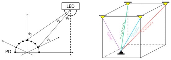
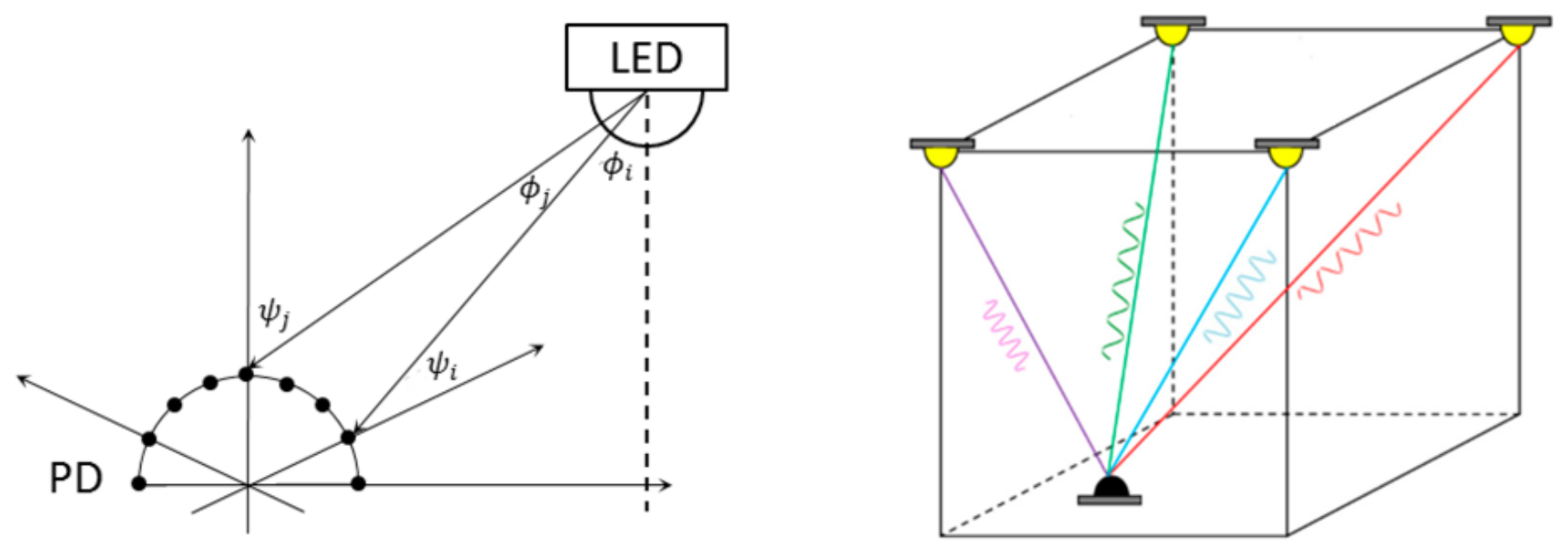
VLP is an infrastructure-based localization system, requiring deployed beacons to function. Within VLP, different localization techniques can be employed. Examples are shown in Figure 1. Time difference of arrival or angle difference of arrival techniques require either synchronized clocks [6] or multiple photodiodes to function [7], thus driving up the costs. Received signal strength (RSS)-based VLP, on the other hand, does not need any synchronized clocks and can be done with a single photodiode as long as the diode can distinguish the light emitted from different light-emitting diodes (LEDs) [7]. This distinction is made possible by modulating the light emitted from the different LEDs at different frequencies, which are also invisible to the human eye. A frequency analysis at the receiver output is then performed to extract the RSS from each LED [8]. The frequency analysis can either be done by a full fast Fourier transform or with techniques built around the Goertzel algorithm [9], which allows for the extraction of specific frequency components chosen beforehand, making for a low-cost design that does not require extensive computation power. Both of these approaches do not require any signal matching between receiver and transmitter, and are hence low-complexity implementations. The obtained RSS can then be used to determine the location of the photodiode within the warehouse with either trilateration techniques or machine learning models. Machine learning (ML) models are particularly useful because they can make up for the non-idealities of the environment, such as multipath propagation, the presence of fixed obstructions, misalignment of the LEDs and their asymmetrical radiation patterns. RSS-based VLP is very precise and has been shown to achieve decimeter-level accuracy [10,11] in 2D applications.
Figure 1.
VLP techniques for localization based on fixed LED positions and tag photodiode(s). On the left: an angle difference of arrival or time difference of arrival approach based on an array of photodiodes. On the right: a received signal strength-based technique relying on a single photodiode with light sources modulated at different frequencies.
The field has grown considerably in recent years, with many experimentally validated VLP prototypes, as discussed in recent survey papers on VLP and visible-light-based indoor localization [12,13,14]. Some of these prototypes even focus on the 3D setting. In [15], a receiver composed of four photodiodes placed behind imaging optics was combined with a neural network, reaching 90th-percentile errors of 3.7 mm in 2D and 51 mm in 3D, the latter within a 540 mm × 540 mm × 120 mm test volume; in [16], a convolutional network trained on the optical power received by four helmet-mounted photodiodes localized personnel within a 6 m × 3 m × 3.6 m underground gallery with a mean experimental error of 11 cm, and did this using only two LEDs (having more photodiodes allows for such a technique); in [17], a single luminaire observed by a low-cost camera yielded real-time 3D estimates with an average error of 4.3 cm in a 2 m × 2 m × 3 m volume, with the image sensor providing the angular information that a bare photodiode cannot. A related camera-based implementation was reported in [18], where a single LED attached to the tracked object was observed by low-resolution ceiling-mounted cameras, with sub-pixel light-spot estimation used to recover the 3D position. It should be noted that these systems rely on image sensors, multiple photodiodes, or comparatively small localization volumes; accurate 3D localization across a large, height-varying industrial space using a single fixed-orientation photodiode remains an open challenge.
VLP in 3D is generally more difficult than in 2D due to the larger search space. Another added complexity of RSS-based VLP in 3D is the presence of dark regions where most if not all LEDs become dim compared to background noise due to their directional propagation characteristics. This problem is at its worst in the corners of the room, which are likely far away from the LEDs, as well as being far away from their main axis of propagation. Though the problem of dark regions is also present in heights that near those of the LEDs, it is at these heights that the light emitted from the LEDs are most concentrated immediately under the LEDs, leaving much of the space dark and significantly reducing positioning accuracy.
The use of ML-based techniques has become quite popular in VLP [19]. In [20], the receiver consists of a single photodiode rotated through a sequence of orientations, in effect replicating a photodiode array with one sensor (albeit at the cost of having to wait for a rotation to obtain a measurement, decreasing the sample rate); this allows localization to be carried out with a single LED, with a random forest first assigning the receiver to an interior or wall-adjacent zone so that the accuracy degradation caused by diffuse wall reflections can be treated separately. Comparative studies between learned and model-based estimators have further shown that, given a careful hyperparameter tuning procedure, feedforward networks can match the accuracy of a maximum-likelihood estimator while substantially reducing prediction time [21]; learned fingerprinting approaches have likewise reached centimeter-level accuracy [22].
The calibration data required by learned models is not negligible, though. In [23], a robotic platform paired with virtual-reality tracking collected RSS measurements at more than 7000 locations to enable a comparison of positioning algorithms; classical model-based positioning was found to remain competitive with learned models when the calibration set is small. Gaussian processes are attractive in this regard, as their Bayesian uncertainty estimates can guide the data collection itself, leading to a better distribution of the data across space, an approach already demonstrated for RSS-based VLP [24]. Kolmogorov–Arnold networks have in turn been investigated for radio-frequency fingerprinting-based localization [25].
In this work, we perform a thorough benchmark of three types of machine learning models with various representations of VLP data collected from a simulator based on the radiation pattern measurements of three VLP LEDs. We find the best combinations by combining Gaussian processes with a logarithmic transformation and multilateration, and show that RSS-based VLP can also achieve high accuracy in 3D under the simulated conditions considered in this work; this strengthens the case for RSS-based VLP in 3D applications, though an experimental validation of the proposed scheme is left for future work. The proposed method is data-efficient and performs well according to all metrics (mean accuracy, 95th percentile precision, etc.) Lastly, we also investigate the impact of varying levels of noise on localization performance and show that our technique is robust down to an SNR of 50 dB, with accuracy degrading gradually at lower SNRs.
Section 2 describes the simulated VLP environment. Section 3 details the data generation process and the considered RSS data representations. Section 4 introduces the machine learning models used for localization. Section 5 provides the implementation details of the models and of the multilateration step. Section 6 presents the results and the noise robustness analysis. Section 7 discusses these results in the context of the existing literature.
2. Simulation Environment
In RSS-based VLP, the RSSs are used to determine the position of the photodiode. This is because real VLP environments pose quite a few challenges that make localization difficult. A non-comprehensive list of such challenges would be reflections; broken lines of sight from LED to photodiode [26]; dust particles in the air and accumulating over time on top of the LEDs or the photodiode surface area; inherent noise coming from ambient light sources; small manufacturing defects that cause LEDs to emit light according to a non-symmetrical radiation pattern; the false assumption that the LEDs are aligned perfectly vertically; etc. Due to the high number of unpredictable conditions in the environment, naive trilateration-based approaches struggle and have lower accuracy compared to algorithms trained on data from the environment [26]. Industry implementations of RSS-based VLP thus rely on data collected from the environment to integrate out the mentioned effects. The collection of said data to adapt model behavior is known as calibration. In [27], the question of how to rely on data to counteract the non-zero and non-negligible tilt of LEDs installed in warehouses is discussed.
In order to collect the data necessary to train and test predictive models using machine learning, we have created a simulation environment that models the behavior of LEDs and photodiodes within a warehouse.
LEDs: Each LED emits light according to its radiation pattern. The LEDs used for VLP are not spherical light sources, but rather a more directional type of light source that emit more light towards the normal direction. They are often modeled as Lambertian light sources [28] that emit light according to a radiation pattern described by the equation:
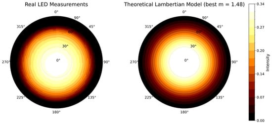
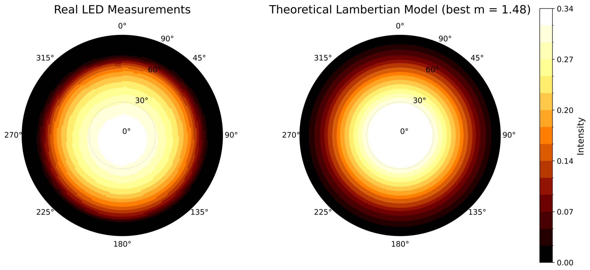
The intensity of light I as a function of the angle with respect to the normal vector of the LED and the distance d is proportional to some power m (called the Lambertian order) of the cosine of , and it also decreases with the square of d. It should be noted that the LED does not emit light towards the half-space that lies behind the normal direction of the LED. A real LED’s radiation pattern also depends on the azimuthal angle . To take this into account, we use measurements of three different real-world LEDs designed for RSS VLP, recording the intensity of light emitted in each direction. The difference in radiation pattern between the hypothetical model and real-life measurements (see Figure 2) can induce drastic accuracy degradations, especially for non-calibrated techniques. In our simulations, we use the real-life measurements of the LED radiation patterns to model the LED behavior. The radiation pattern data used in this work is from Xicato LED modules and is collected using a TechnoTeam Bildverarbeitung GmbH, Ilmenau, Germany RiGO801-L near-field goniophotometer (KU Leuven Light & Lighting Laboratory: https://iiw.kuleuven.be/onderzoek/lichttechnologie/english/equipment/nearfieldgoniophotometer, accessed on 11 July 2026). The radiation intensity is measured at every interval for all and combinations and is linearly interpolated to obtain a continuous radiation pattern.
Figure 2.
The manufacturing process results in asymmetries in how much light a real LED emits in each direction. On the left, the measured values for an LED manufactured for VLP purposes using a photo goniometer; on the right, a calibrated Lambertian radiation pattern that best matches the measurements for the same LED.
Photodiodes: The light emitted from each of the LEDs is captured by the photodiode, which can be located anywhere within the warehouse with any orientation, though in our experiments the diode surface area is restricted to always point upward. This sets the scope for our localization technique, which is in three spatial dimensions without taking into account the three extra dimensions that come from orientation.
The received signal strength of the LED with radiation pattern is calculated with:
where is simply the angle the LED has with respect to the normal direction of the photodiode and A represents the sensor’s sensitivity, active surface area and related constants. It should be noted that the values of such parameters are not individually consequential for the localization performance reported in this work, as they only affect the resulting RSS measurements multiplicatively. Their effect can thus be captured by the resulting signal-to-noise ratio (SNR). We therefore fix them to representative values and treat the SNR as the determining variable.
3. Data Generation and Representation
In this section, we describe how training and test data of our models is obtained.
3.1. The Room Configuration
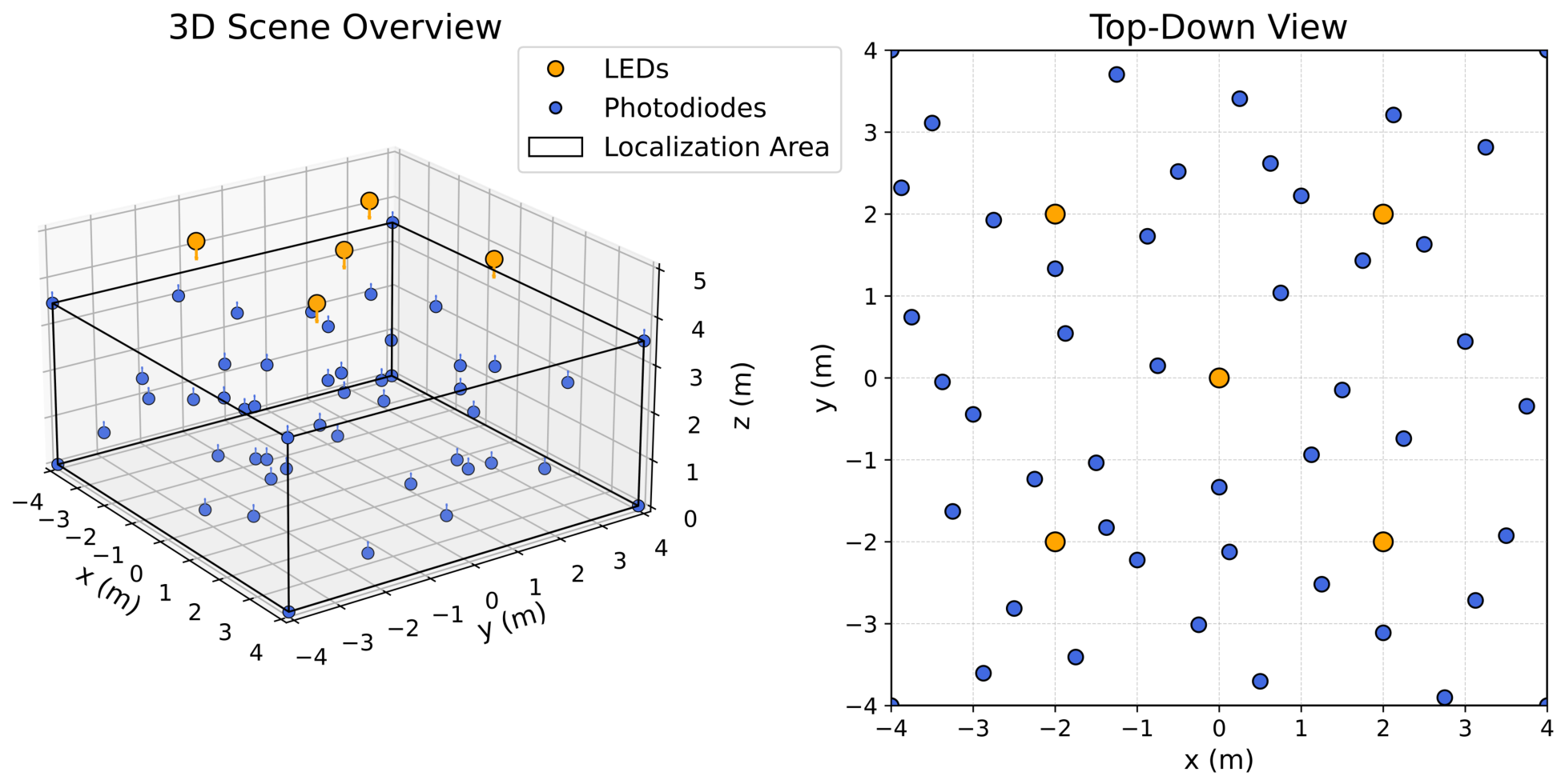
For testing the performance of RSS-based VLP in 3D, we consider a warehouse of 8 m × 8 m surface area with five LEDs placed at the ceiling at a height of 5 m with respect to the ground. One LED is placed at the center of the ceiling and the others are placed at the corners of a 4 m × 4 m square centered around the first and aligned with the walls. Localization in this warehouse is a challenge due to its large size. Due to the directional nature of the LED radiation patterns, the upper corners of the room are the darkest locations in the room, making accurate localization even more challenging. At heights near the ceiling, most of the locations receive practically no light from any of the LEDs, thus making RSS-based VLP infeasible. To combat this, we restrict the localization volume to the 8 m × 8 m × 3.5 m rectangular cuboid.
3.2. Sampling Technique
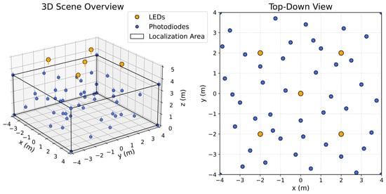
Training Data: The training data is sampled in a point-wise manner. The training samples contain no Gaussian noise because we assume that the photodiode can be halted for oversampling during calibration. An oversampling rate of four is enough to bring the SNR from 40 dB (worst-case scenario in practical settings) to 60 dB (where we later show that model performance is unimpaired compared to no noise). As for the sample locations, we use a space-filling Halton sequence to capture the global structure of the input-output mapping [29]. Samples from the eight corners of the room are also included in the training data to reduce the areas where the models must extrapolate. The warehouse configuration, as well as the sampling scheme, can be observed in Figure 3, where each photodiode shown corresponds to a location where the RSS from each LED is recorded. We report the findings for models trained on 50–400 training samples.
Figure 3.
The warehouse configuration for the localization scheme contains five LEDs all placed at the same height of 5 m above ground level. Localization is restricted only in the zone inside the cuboid where the height is less than 3.5 m. The LED radiation patterns come from measurements of real world LEDs. The sampling scheme includes samples on the boundaries of the room as well as space-filling samples according to the Halton sequence. The figure depicts eight corner samples and 42 Halton samples.
To test the robustness of our models, we generate 10 datasets per training size (ranging from 50 to 400 samples) according to different Halton seeds.
Test Data: To test the performance of the trained ML models, we collect samples in a fine grid according to a crystal of 50 × 50 × 50 samples along the three spatial dimensions.
These data are corrupted with varying levels of noise to quantify model performance under noisy environments. This corresponds to the scenario where we cannot rely on oversampling to reduce the effects of the additive noise (e.g., if the vehicle is moving). To this end, we fix the central LED and the floor of the localization area as baseline and tune the noise variance such that an average SNR of 60, 50, 40 and 30 dB is obtained.
We later provide the performance of our best model type under noisy and noiseless conditions to show the effects of added noise on localization accuracy.
3.3. Data Representations
In this paper, we address three possible transformations of the data and investigate their effects on model performance.
Absolute Representation: This is the most basic approach as it involves making no changes to the data apart from standardization. The received signal strengths from all the LEDs (five in our case) are used as inputs to the model and the models are trained to predict the x, y, and z locations in 3D space.
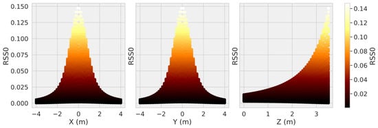
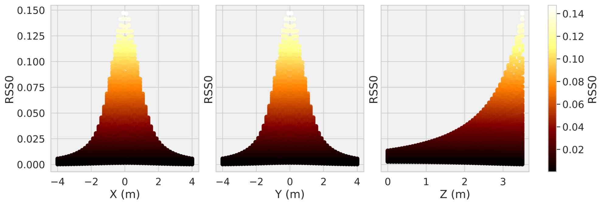
Figure 4 shows the pair plots between RSS from the central LED and the output features (position). Higher RSS generally corresponds to higher heights, although the relationship is non-linear. The data shown in this plot comes from the dense sampling used for the test set, training datasets include significantly fewer data points.
Figure 4.
Pairplots between the intensity of the central LED and the x, y, and z coordinates. The closer we are to the center of the room (right underneath the central LED), the higher the RSS. The higher we are in height (and thus closer to the LED), the higher the RSS.
The model input and outputs are
Relative Representation: The warehouses in which the photodiodes must be used for localization do not always have stationary conditions. Dust and other particles in the air may affect the transmittance of the air and these same particles may accumulate on the photodiode over time, resulting in reduced and thus faulty received signal strength measurements. Aside from continual calibration, another way to combat this would be to engineer features that inherently resist this type of degradation. The ratio of two received signal strengths is one such feature. Under the assumption that small dust particles can be modeled as casting a uniform shadow on the photodiode surface in an isotropic manner, all received strengths will be affected by the same transmittance. For a total of n LEDs, we may form pairs of distinct LEDs whose received signal strength ratios can be used as features for model training. The model inputs and outputs are
LogD Representation: The signal strength received from an LED gives us information on the photodiode’s distance to that LED. In the case of perfectly spherical light sources, this relation is a bijection assuming the photodiode is always pointed towards the LED. According to the inverse-square law and one calibration point, one may recover the distance to the LED based on the measured RSS. If this can be done for at least four LEDs and the locations of these four LEDs are known, then the position of the photodiode can be determined by multilateration.
The LEDs used for VLP, however, are not spherical and the photodiode orientation is also restricted to always remain pointing upwards. For this reason, the relationship between RSS and distance to LED is not a bijection. However the inverse-square propagation law persists along each direction, such that higher RSS likely means lower distance. Approaches based on estimating no longer the exact but the expected distance to the LED given the measured RSS have been used for VLP in the past, though models trained on the absolute data as discussed earlier have been shown to outperform this naive multilateration approach. This is because this approach does not take into account the asymmetries of the LEDs and the imperfections of the environment and base their multilateration scheme on a Lambertian modeling of the LEDs, resulting in poorer performance.
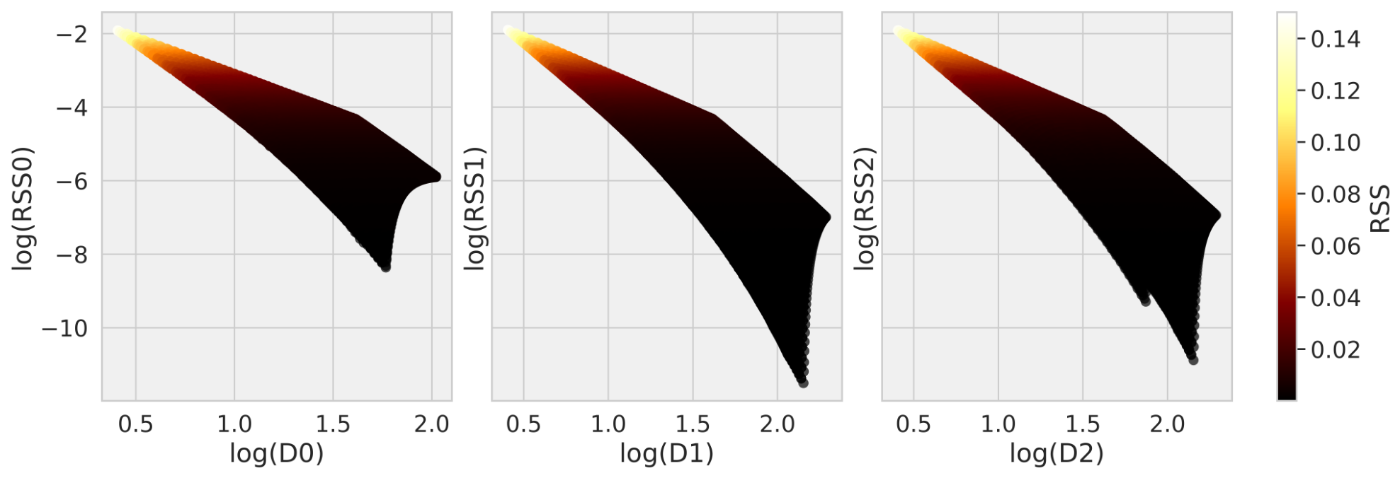
A different approach is to use machine learning models to predict the distances to the LEDs based on the RSS. This allows for the prediction of the distance to each LED to also take advantage of the knowledge of the RSS from other LEDs, and the asymmetries and imperfections of the environment will be learned through the data. To do this, we apply the following preprocessing step to the data which puts input features (RSS) in an (almost) linear relationship with the corresponding output features (distance to LEDs) according to the inverse square law:
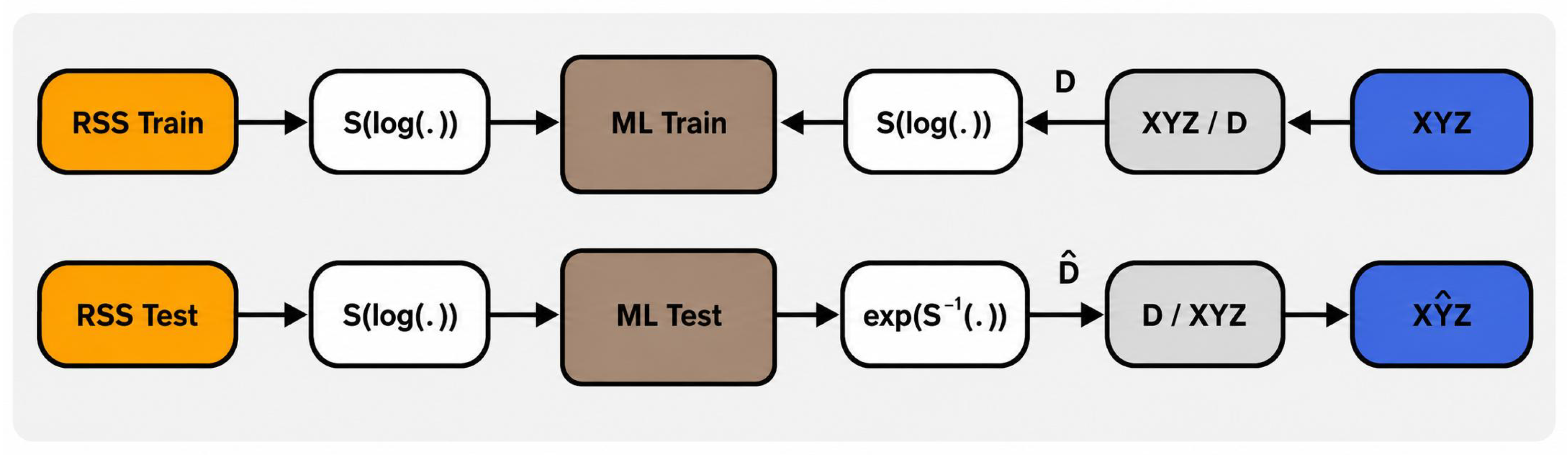
This (almost) linear relationship between corresponding input and output features for the same LED can be seen in Figure 5. This linearity is broken by non-isotropic radiation patterns and may be further broken by noise or reflections/refractions. The global localization scheme for models using this preprocessing of the data, including the multilateration step to obtain the XYZ, is shown in Figure 6. The multilateration step uses the known locations of the LEDs and is based on gradient descent. The multilateration was tested for accuracy and produces a worst-case error below 0.5 mm at the worst possible case (assuming the correct distances were output by the model). Any error at the output thus stems from the ML models.
Figure 5.
Pairplots between the logarithms of received signal strength and distance to the same LED.
Figure 6.
The logD models are trained to use the logarithms of RSS to predict the logarithms of distances to LEDs. At evaluation, the model outputs are converted back into the XYZ domain with multilateration based on distances to LEDs.
4. Machine Learning Models
In the proposed RSS-based VLP scheme, ML models are used to capture the relationship between the input and the output data. In its simplest form, this would be an ML model that takes the RSS measurements from all the LEDs as input and yields the x, y, and z location predictions as output. We consider three types of ML models:
Gaussian Processes (GPs): GPs are probability distributions over functions and provide a Bayesian framework for modeling the input–output behavior of functions. This is done by combining a prior distribution over functions, with a covariance matrix (a.k.a. kernel) that correlates the outputs of inputs that are close to each other in the input space, with the sampled input–output data to obtain a posterior distribution over functions. This posterior predictive distribution not only has a mean that we can use as the prediction but also an uncertainty, providing information on how certain the model is about its prediction for a certain input. This information can be used to guide the data-collection process towards more informative samples in what is more generally known as Bayesian Optimization or Active Learning and has already been implemented for RSS-based VLP [24].
Neural Networks (NNs): NNs are a basic yet powerful type of feedforward neural network composed of multiple layers of interconnected nodes [30]. Each node applies a learned linear transformation to its inputs, then passes the result through a non-linear activation function. The successive composition of such linear transformation + non-linear activation functions remains a differentiable function, meaning that gradient-descent-based methods can be used to teach the input–output behavior of the data to the model (e.g., from RSS measurements to predicted location) [31].
Kolmogorov–Arnold Networks (KANs): KANs are a relatively new type of machine learning model and are inspired by the Kolmogorov–Arnold representation theorem [32]. This theorem states that any continuous multivariate function can be expressed as a finite sum of univariate nonlinear functions applied to linear combinations of the inputs. In contrast to NNs, where the nonlinear activation functions (placed on the nodes) are fixed and it is the weights and the biases that must be tweaked for the model to learn, in KANs, it is these activation functions (placed on the edges) that must be learned and the nodes serve only for summation. One attractive point is the interpretability of the final trained models as the trained models can often be pruned before undergoing some slight retraining to give a functional representation of the input–output behavior of the data [33].
5. Materials and Methods
The simulation environment based on real-life LED radiation pattern measurements as well as the data sampled at various noise levels are made available at GitHub. The model training procedure and pretrained models are also provided so that the study can be fully reproduced.
5.1. Multilateration Implementation
For the LogD representation, the machine learning models predict the distances from the photodiode to the LEDs. These predicted distances are then converted to spatial coordinates by a multilateration step. This step is implemented as a bounded least-squares optimization problem using the L-BFGS-B algorithm [34], as implemented in SciPy [35].
Let denote the model-predicted distance to the ith LED, and let denote the known position of that LED. The estimated photodiode position is obtained by minimizing the mean squared distance residual
where n is the number of LEDs and denotes the imposed bound constraint. In our implementation, the only active bound is
This constraint is necessary due to the fact that all LEDs lie on the same plane (the ceiling), meaning that there are always two solutions possible to a set of given distances to the LEDs, one on each side of the plane. The constraint simply eliminates the solution which lies above the ceiling. The horizontal coordinates are left unbounded. The optimization is initialized at the centroid of the LED positions. The default L-BFGS-B convergence settings of SciPy were used in our implementation, corresponding to a relative reduction tolerance of approximately , a projected gradient tolerance of , and a maximum of 15,000 iterations.
Since the considered setup contains five LEDs and only three unknown spatial coordinates, the multilateration problem is over-determined. This makes the solution less sensitive to individual distance prediction errors than a minimally determined system, although systematic errors in the predicted distances can still bias the final position estimate. Across the full test grid, no convergence failures were observed when using the centroid initialization.
To verify that the multilateration step itself does not introduce a significant numerical error, we also evaluated it using the ground-truth distances from the test locations to the LEDs. In this case, the worst-case localization error introduced was below mm. The localization errors reported in Section 6 are therefore caused by model predictions.
5.2. GP Training
The GPs in this work are all implemented as standard exact GP regression with a zero mean function and a Squared Exponential kernel (such that the GP is a universal approximator) with automatic relevance determination in the gpflow library. Each input dimension carries its own length scale, giving five length scales for the Absolute and LogD representations and 10 for the Relative representation. GPs being non-parametric ML models, the free hyperparameters are jointly optimized by maximizing the log marginal likelihood with gpflow’s wrapper around SciPy’s L-BFGS-B implementation. The optimization is initialized with 0.2 for all length scales and a noise variance of , with the default gpflow initial kernel variance; since the inputs are pre-standardized to unit variance, a length scale of 0.2 corresponds to roughly 20 percent of the input scale, though this value was not further tuned. The optimizer terminates under SciPy’s default L-BFGS-B convergence criteria (relative reduction in the negative log marginal likelihood below approximately , gradient norm below , or a maximum of 15,000 iterations). For all three representations the GP is trained as a multi-output model with the kernel and its hyperparameters shared across output dimensions.
5.3. NN Training
The neural networks are implemented in TensorFlow/Keras and share an architecture across the three data representations: an input layer matching the representation’s feature dimension, two fully connected hidden layers of 15 units each with ReLU activations, and a linear output layer matching the target dimensionality (three outputs for Absolute and Relative, five outputs for LogD). Weight initialization is done according to Glorot uniform sampling for the kernels and zero for the biases, which are the default Keras defaults.
We train each network by minimizing the mean squared error between predicted and true targets using the Adam optimizer with its Keras default hyperparameters (eta = , = 0.9, = 0.999, epsilon = ), a batch size of 250, and a fixed number of training epochs: 20,000. In every configuration, the training loss was observed to plateau well before the chosen epoch limit.
The architectures and optimizer settings were kept identical across the three representations, with only the input and output dimensions adapted to each one; this was a deliberate choice, since the comparison of interest in this work is across the data representations and across the model classes, and applying the same configuration throughout ensures that any performance differences reflect the data representation and the model class rather than differences in tuning effort. A more thorough sweep of width, depth, activation, or learning rate could improve the NN’s performance further in each representation.
5.4. KAN Training
We use the reference pykan implementation of KANs. The architecture has the form : a single hidden layer of three KAN nodes connecting an input layer of size matching the representation to an output layer of size matching the target dimensionality. The learnable activations on each edge are based on B-splines of degree k = 3. Following the pykan grid-refinement procedure, training proceeds in two stages: we first train with a B-spline grid size G = 3 for 30,000 optimizer steps, then call on refine(10) to upsample the splines to G = 10 and train for another 30,000 steps. Both stages use pykan’s internal Adam optimizer with learning rate and a batch size of 128. The training losses were observed to plateau long before the optimizer steps expired at each stage.
As with the NN, the same architecture and hyperparameters are used across all three representations to maintain a controlled comparison; a more targeted KAN hyperparameter search could likewise improve performance in each representation.
The computation times reported in this study were carried out on a workstation equipped with Intel® Core™ Ultra 7 165U, 12 cores, 16 GB DDR5 RAM. Software versions used were Python 3.12.3, TensorFlow 2.16.2, gpflow 2.11.0, and pykan 0.2.8. It should be noted that NN training times could be reduced by training on GPUs, whereas the computations required to train a KAN do not parallelize to the same extent across multiple cores.
6. Results
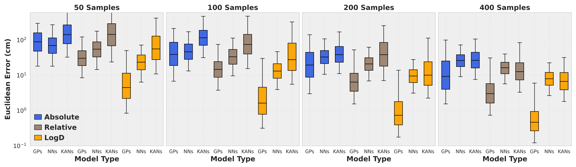
The error distribution for the different models is shown in Figure 7. Two observations can be made. The first is that within each data representation, the GP models seem to perform the best among the three types of ML models tested. The second is that among each type of ML model, the LogD representation of the data appears to be the best when it comes to accuracy. The combination of a GP model and a logD representation for the data is consistently the best.
Figure 7.
Prediction error in Euclidean distance of every type of model trained on every representation of the data for models trained on 50, 100, 200 and 400 training samples.
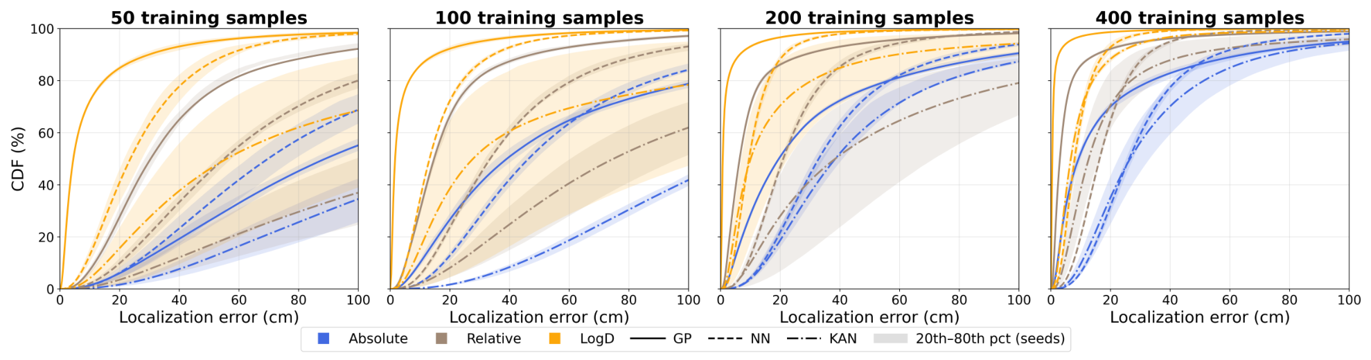
Additionally, the higher levels of accuracy achieved by the GPs are robust to different random Halton samplings. In contrast, NN and KAN performance may vary significantly based on different random parameter initialization and where the samples are taken. This can be observed in Figure 8 where the NNs and KANs have high variance in model performance, whereas the GP performance is robust. Although each GP received data sampled at different locations, they all have similar levels of accuracy. In contrast to GPs, both NN- and KAN-based ML models exhibited lower levels of accuracy, as well as more variability in model performance conditioned on different random initial samples and the initialization of the network parameters. A numerical representation of Figure 8 can be found in Appendix A.
Figure 8.
Cumulative error distribution based on Euclidean distance for all types of models. Lines show the mean CDF across the 10 different seeds (training samples at different locations, as well as different random model initialization); shaded bands span the 20th–80th percentile. Each of these 10 models also received a different set of Halton random samples in their training data.
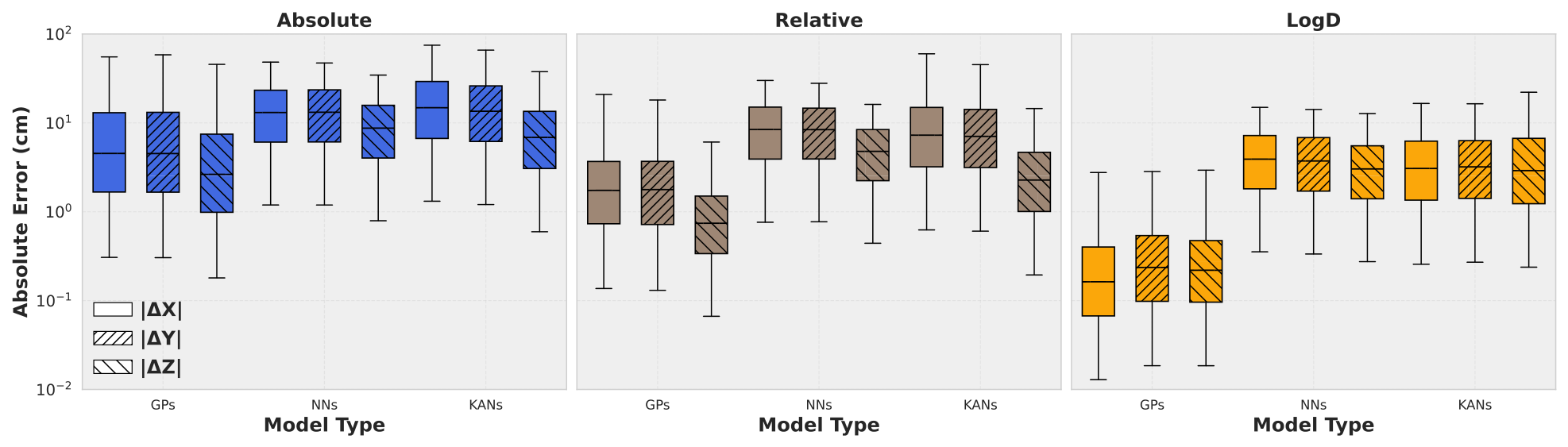
Decomposing the Euclidean error made by the models along the x, y, and z axes (z being the vertical axis) shows that the localization scheme favors localization along the vertical dimension, as shown in Figure 9. We can expect a difference in performance when comparing the z axis to the x and y axes because the LEDs are pointing from top to bottom, and also the localization height is limited to 3.5 m compared to the full 8 m along the other dimensions. Interestingly, however, using the LogD representation of the data seems to eliminate this asymmetry, causing model performance to be very similar along all three dimensions. It is unclear, however, whether this behavior is specific to the considered configuration.
Figure 9.
Breakdown of the error of every type of model along each spatial direction. The configuration (room size, LED positioning) shows a general favor towards the z axis as the models have significantly smaller errors along this direction apart from the LogD models.
It should be added that the additional accuracy achieved by the logD implementation comes with additional computational cost, as it requires an extra step of multilateration at the output, potentially slowing down the sample acquisition rate and responsiveness of localization. The runtimes for model inference are given in Table 1 where we can observe that multilateration slows down model inference by three orders of magnitude. However, it should be stated that our implementation of multilateration was not built with speed in mind and significantly faster multilateration speeds may be achieved by adding optimized solvers or closed-form initialization strategies. Regardless, when implementing the logD-based technique for VLP, more thought needs to be given to the speed of the multilateration if inference time is the bottleneck of the sample rate.
Table 1.
Mean inference time of models and the added time to convert log distances to spatial coordinates with multilateration. These models were trained on 400 samples.
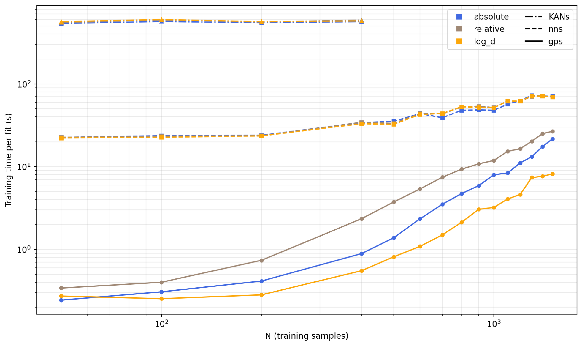
The three types of models compared in this work scale differently. Training an exact GP on n calibration points requires the Cholesky factorization of an matrix, which comes at in computation time; the posterior mean can then be inferred at an computation cost and the predictive uncertainty at an computation cost. NNs and KANs, on the other hand, are trained with stochastic gradient descent, meaning that the training cost can either be set in terms of a fixed number of optimizer steps (as we have done with the KANs, see Section 5.4) or in terms of a fixed number of epochs (as for the NNs). The training cost is then —independent of n—or , respectively, where P represents the number of network parameters being updated. Representative training times for individual models across all three model classes can be seen in Figure 10. Though the cubic scaling factor of the Cholesky decomposition is not yet dominating for the small dataset sizes that we consider, it is clear that the exact GP training time may impose scalability restrictions, especially if one is working with dense datasets or with localization areas much larger than the one reported in this study. That said, given that calibration only takes place once or upon every recalibration step, we posit that exact GPs can be adequate for datasets of up to 4000 samples. For larger datasets, a sparse variational GP is recommended, which introduces inducing points and reduces the computational cost of training to while preserving the ability to output a Bayesian uncertainty metric. An interesting observation is that the LogD GPs appear to finish training approximately three times faster than their absolute and relative counterparts. We suspect this is due to the linearizing effect of the logarithmic transform on the input–output relationship; the L-BFGS-B algorithm responsible for the hyperparameter optimization is likely working within a smoother landscape and is able to converge in fewer iterations.
Figure 10.
Average training time required for each individual model based on model type and data representations. Exact GP training time expected to scale cubically with training data size, though this regime is not yet attained with these dataset sizes.
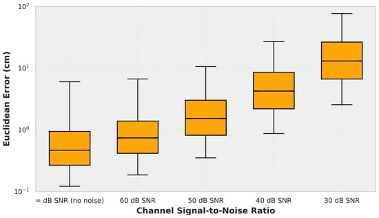
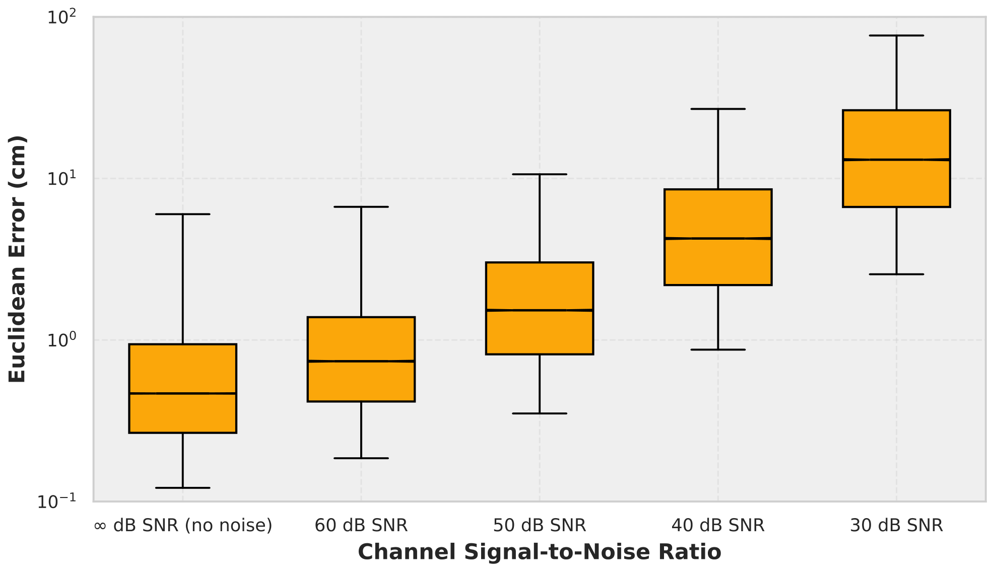
Finally, the impact of noise on model performance for the LogD-GPs can be seen in Figure 11 where significant accuracy drops below 50 dB SNR. The LogD-GPs can achieve a p95 of 10 cm in 50 dB SNR environments given the 400 training samples in our setup. A comparison between our work and VLP systems reported in the literature is summarized in Table 2. It should be noted that these systems differ in room dimensions, number of LEDs, localization volume, SNR conditions, receiver type, and validation methodology (simulation versus experiment); Table 2 therefore situates our results within the broader performance landscape rather than constituting a controlled benchmark.
Figure 11.
Noise can impact the performance of the models; this figure shows how the performance of models trained on 400 training samples fared against noise.
Table 2.
Comparison of RSS-based VLP systems reported in the literature with the GP-LogD models trained on 400 samples. The listed systems differ in geometry, LED count, SNR conditions, receiver type, and validation methodology; the reported errors are indicative rather than directly comparable.
7. Discussion
Within RSS-based VLP, there are many different techniques available. In [18], a single LED is attached to the object to be tracked with 12 low resolution image sensors placed on the ceiling (the inverse of our setup) and they perform localization in a 1 m × 1 m surface area at fixed height and report a 3D localization error of 2.5 cm.
In [37], the challenging task of performing localization and orientation simultaneously is undertaken. The localization and orientation are performed in a 9 m × 9 m × 4 m room (very similar to ours) with a similar setup, a photodiode that captures RSS from LEDs placed on the ceiling. The SNR of the signal from each LED was reported to be at around 20 dB in the study and they relied on a total of 81 LEDs to do the localization. The study is also simulation-based but relies on a Lambertian hypothesis. Based on the Lambertian hypothesis, they derive a closed-form algorithm for localization and are not data-reliant. The similar room sizes make this comparison relevant, as they report having a p95 accuracy of 21 cm. However, this is a significant accomplishment given that they localize the photodiode under different orientations than just upward-facing. Regardless, with the high number of LEDs used in the study, they are able to manage such accuracies. One drawback of their closed-form expression, however, is that the time it takes to obtain the position and orientation was reported to be more than two seconds on their system. This is orders of magnitude greater than the sampling rate found in photodiodes used for RSS-based VLP which is bound to be the bottleneck in the loop. Our proposed technique, on the other hand, takes less than 10 ms in the worst case to perform the localization, with the majority of time being spent performing multilateration which can further be reduced.
In [39], the setup is also similar to ours, with the object to be localized equipped with a single upward-pointing photodiode with LEDs placed on the ceiling. The LEDs are modulated at different frequencies, allowing for the distinction at the receiver to calculate the RSS used to localize the photodiode. Their method is based on equations derived from the Lambertian hypothesis for the LEDs and thus requires little calibration in comparison to our technique. A disadvantage of this type of approach is that multipath reflections have a large negative impact on the positioning accuracy. They test their technique in two separate room configurations. The first is a large 25 m × 15 m × 5 m room with a total of 15 LEDs placed on the ceiling in a grid formation. In a simulation where they also take into account the secondary light paths (something which their algorithm does not take into account as it is not data-based), they achieve a p90 accuracy of 30 cm, and they experimentally verify this p90 accuracy, measuring 36 cm. The same technique is also tested in an 4 m × 4 m × 4.1 m room where the photodiode ranges from a height of 0.64 m to 2.55 m, both in a simulation environment and a real experiment and report p90 accuracies of 4 cm and 24 cm, respectively. The large difference between the two results is explained by the non-ideal radiation pattern of the LEDs and mainly the multi-path reflections which were not accounted for in this study due to the non-trivial perimeter of the room. They report that the SNR values for LEDs ranged from 83 dB to 19 dB at different locations in the small room setup, the computation time for position estimation is not mentioned. The approach developed in this study can form the basis of a good baseline on top of which calibration-based ML models may be added for extra data efficiency, but the large drop in accuracy caused by secondary paths is precisely why calibration-based techniques such as ours are favored in industrial applications. Taken together, these comparisons serve to position our results within the existing literature; a like-for-like comparison would require evaluating the different approaches on a common geometry and dataset, which the public release of our algorithm and simulation framework is intended to facilitate.
We propose a 3D VLP simulation framework based on the radiation patterns of real LEDs. In our contributions, we demonstrate that ML models trained to predict distances to the LEDs based on LogD data followed by a multilateration step perform significantly better than training the models to predict spatial coordinates. With our proposed technique, 400 training samples from five LEDs were sufficient to achieve a p95 error of 10 cm and an average error of 3.7 cm in a space of 8 m × 8 m × 3.5 m dimensions with an average SNR of 50 dB for the central LED.
These findings indicate that single-photodiode RSS-based VLP is viable for height-varying scenarios. However, this requires knowledge or a good estimate of the position of the LEDs as well as the processing power to perform multilateration. The multilateration occurs after the ML models have made their predictions and thus cannot be calibrated, hence the importance of precise knowledge of their location. The multilateration algorithm also needs to be designed with speed in mind so as to not cause a bottleneck in sampling rate. We show that the performance of RSS-based VLP in 3D can approach 2D applications and is applicable under the simulated conditions considered here.
It should be noted that the validation presented in this work is entirely simulation-based. The simulator was designed to remain close to a practical deployment, relying on measured radiation patterns, a warehouse-scale geometry, and noise levels resembling those of real warehouses; effects such as multipath reflections and LED tilt are nevertheless not modeled. Since the proposed scheme is calibration-based, such non-idealities would be reflected in the collected training data and are expected to be at least partially absorbed by the models, as is already the case for the radiation–pattern asymmetries considered here; there are, however, non-idealities which are more difficult for ML models to absorb from the data, such as a non-stationary photodiode tilt. Quantifying this absorption requires measurements on a physical testbed, which is the natural next step of this work.
Author Contributions
This research was conducted by A.N.K. under the supervision of I.C. and T.D. and the domain expertise of N.S. Conceptualization, all authors; data curation, N.S.; formal analysis, A.N.K.; funding acquisition, I.C. and T.D.; investigation, A.N.K.; methodology, A.N.K., I.C. and T.D.; project administration, I.C. and T.D.; resources, T.D. and I.C.; software, A.N.K.; supervision, I.C. and T.D.; validation, A.N.K.; visualization, A.N.K.; writing—original draft, A.N.K.; writing—review and editing, all authors. All authors have read and agreed to the published version of the manuscript.
Funding
This work was supported by the Flemish Government under the “Onder-zoeksprogramma Artificiele Intelligentie (AI) Vlaanderen”. This research is financially supported by the Research Foundation—Flanders (FWO) (grant number G0A2824N).
Data Availability Statement
The original data presented in the study are openly available at https://github.com/Arman-Gent/RSS-based-VLP (accessed on 20 May 2026) under an MIT license.
Acknowledgments
We would also like to thank Frederic Leloup, Jan Audenaert and Wouter Ryckaert from the KU Leuven Light and Lighting Laboratory for taking the LED radiation pattern measurements. During the preparation of this manuscript, the author Arman N.K. used ChatGPT (GPT-4o, OpenAI) for the purposes of writing and debugging code, as well as generating the figures depicted in this work. The authors have reviewed and edited the output and take full responsibility for the content of this publication.
Conflicts of Interest
The funders had no role in the design of the study; in the collection, analyses, or interpretation of data; in the writing of the manuscript; or in the decision to publish the results. Authors Arman Nikraftar Khiabani, Tom Dhaene and Ivo Couckuyt were employed by IMEC. The remaining authors declare that the research was conducted in the absence of any commercial or financial relationships that could be construed as a potential conflict of interest.
Abbreviations
The following abbreviations are used in this manuscript:
| VLP | Visible light positioning |
| RSS | Received signal strength(s) |
| LED | Light-emitting diode |
| SNR | Signal-to-noise ratio |
| GP(s) | Gaussian process(es) |
| NN | Neural network |
| KAN | Kolmogorov–Arnold network |
| ML | Machine learning |
| CDF | Cumulative distribution function |
Appendix A
In the appendix, we report the mean and p95 errors committed by our models across the localization space using the test data. The confidence intervals, calculated based on the 10 separate datasets, are also provided to show how random model initializations and data acquisition locations can impact performance.
Table A1.
Mean Euclidean localization error by data representation, model type, and number of training samples. Values are reported in centimeters as mean [95% confidence interval] over ten randomized training sets.
Table A2.
The 95th-percentile Euclidean localization error by data representation, model type, and number of training samples. Values are reported in centimeters as mean [95% confidence interval] over ten randomized training sets.
References
- Sesyuk, A.; Ioannou, S.; Raspopoulos, M. A Survey of 3D Indoor Localization Systems and Technologies. Sensors 2022, 22, 9380. [Google Scholar] [CrossRef] [Scilit] [PubMed]
- Lymberopoulos, D.; Liu, J.; Yang, X.; Choudhury, R.R.; Handziski, V.; Sen, S. A realistic evaluation and comparison of indoor location technologies: Experiences and lessons learned. In IPSN’15: Proceedings of the 14th International Conference on Information Processing in Sensor Networks; Association for Computing Machinery: New York, NY, USA, 2015; pp. 178–189. [Google Scholar] [CrossRef] [Scilit]
- Aziz, T.; Koo, I. A Comprehensive Review of Indoor Localization Techniques and Applications in Various Sectors. Appl. Sci. 2025, 15, 1544. [Google Scholar] [CrossRef] [Scilit]
- Zhu, Z.; Guo, C.; Bao, R.; Chen, M.; Saad, W.; Yang, Y. Positioning Using Visible Light Communications: A Perspective Arcs Approach. arXiv 2022, arXiv:2204.08131. [Google Scholar] [CrossRef] [Scilit]
- Bastiaens, S.; Alijani, M.; Joseph, W.; Plets, D. An experimental analysis of visible light positioning in NLoS environments. In Work-in-Progress Papers at the 13th International Conference on Indoor Positioning and Indoor Navigation (IPIN-WiP 2023); Kaiser, S., Franke, N., Mutschler, C., Eds.; CEUR: Aachen, Germany, 2023; Volume 3581, p. 13. [Google Scholar]
- Cincotta, S.; He, C.; Neild, A.; Armstrong, J. High angular resolution visible light positioning using a quadrant photodiode angular diversity aperture receiver (QADA). Opt. Express 2018, 26, 9230–9242. [Google Scholar] [CrossRef] [Scilit] [PubMed]
- Bakar, A.H.A.; Glass, T.; Tee, H.Y.; Alam, F.; Legg, M. Accurate Visible Light Positioning Using Multiple-Photodiode Receiver and Machine Learning. IEEE Trans. Instrum. Meas. 2021, 70, 7500812. [Google Scholar] [CrossRef] [Scilit]
- Wang, Q.; Luo, H.; Gao, X.; Wei, J.; Zhao, F. An Indoor Three Dimensional Positioning Algorithm Based on Attitude Identification and Visible Light Propagation Model. In China Satellite Navigation Conference (CSNC) 2017 Proceedings: Volume I; Sun, J., Liu, J., Yang, Y., Fan, S., Yu, W., Eds.; Springer: Singapore, 2017; pp. 367–380. [Google Scholar] [CrossRef] [Scilit]
- Goertzel, G. An Algorithm for the Evaluation of Finite Trigonometric Series. Am. Math. Mon. 1958, 65, 34–35. [Google Scholar] [CrossRef] [Scilit] [PubMed]
- Raes, W.; De Strycker, L.; Stevens, N. Design and Accuracy Evaluation of a RSS-Based Visible Light Positioning Implementation. In Proceedings of the 2018 15th Workshop on Positioning, Navigation and Communications (WPNC), Bremen, Germany, 25–26 October 2018; pp. 1–5. [Google Scholar] [CrossRef] [Scilit]
- Bai, L.; Yang, Y.; Feng, C.; Guo, C. Received signal strength assisted perspective-three-point algorithm for indoor visible light positioning. Opt. Express 2020, 28, 28045–28059. [Google Scholar] [CrossRef] [Scilit] [PubMed]
- Rahman, A.B.M.M.; Li, T.; Wang, Y. Recent Advances in Indoor Localization via Visible Lights: A Survey. Sensors 2020, 20, 1382. [Google Scholar] [CrossRef] [Scilit] [PubMed]
- Bastiaens, S.; Alijani, M.; Joseph, W.; Plets, D. Visible Light Positioning as a Next-Generation Indoor Positioning Technology: A Tutorial. IEEE Commun. Surv. Tutor. 2024, 26, 2867–2913. [Google Scholar] [CrossRef] [Scilit]
- Wang, R.; Niu, G.; Cao, Q.; Chen, C.S.; Ho, S.W. A Survey of Visible-Light-Communication-Based Indoor Positioning Systems. Sensors 2024, 24, 5197. [Google Scholar] [CrossRef] [Scilit] [PubMed]
- Apolo, J.A.; Osahon, I.N.O.; Ortega, B.; Almenar, V.; Tang, J.; Rajbhandari, S. Experimental Demonstrations of High-Accuracy 3D/2D Indoor Visible Light Positioning Using Imaging Multiple-Input Multiple-Output Receivers and Artificial Neural Networks. IET Optoelectron. 2025, 19, e70000. [Google Scholar] [CrossRef] [Scilit]
- Deng, B.; Wang, F.; Qin, L.; Hu, X. A Visible Light 3D Positioning System for Underground Mines Based on Convolutional Neural Network Combining Inception Module and Attention Mechanism. Photonics 2023, 10, 918. [Google Scholar] [CrossRef] [Scilit]
- Ma, Z.; Li, J.; Fan, X.; Zeng, J.; Cao, H.; Zhou, B.; Pan, H.; Fang, J. A high-speed and high-accuracy single LED three-dimensional visible light positioning system based on virtual beacon. Opt. Commun. 2025, 578, 131479. [Google Scholar] [CrossRef] [Scilit]
- Khan, S.; Paradells, J.; Catalan, M. Low-Cost 3D Indoor Visible Light Positioning: Algorithms and Experimental Validation. Photonics 2024, 11, 626. [Google Scholar] [CrossRef] [Scilit]
- Rekkas, V.P.; Iliadis, L.A.; Sotiroudis, S.P.; Boursianis, A.D.; Sarigiannidis, P.; Plets, D.; Joseph, W.; Wan, S.; Christodoulou, C.G.; Karagiannidis, G.K.; et al. Artificial Intelligence in Visible Light Positioning for Indoor IoT: A Methodological Review. IEEE Open J. Commun. Soc. 2023, 4, 2838–2869. [Google Scholar] [CrossRef] [Scilit]
- Liu, R.; Liang, Z.; Yang, K.L.; Li, W. Machine Learning Based Visible Light Indoor Positioning With Single-LED and Single Rotatable Photo Detector. IEEE Photonics J. 2022, 14, 7322511. [Google Scholar] [CrossRef] [Scilit]
- Martins, R.; Mathias, L.; Abrão, T. 3-D Indoor Visible Light Positioning Using Machine Learning and Hyperparameter Tuning. J. Netw. Syst. Manag. 2025, 33, 79. [Google Scholar] [CrossRef] [Scilit]
- Xu, S.; Wu, Y.; Wang, X.; Wei, F. Indoor High Precision Positioning System Based on Visible Light Communication and Location Fingerprinting. J. Light. Technol. 2023, 41, 5564–5576. [Google Scholar] [CrossRef] [Scilit]
- Glass, T.; Alam, F.; Legg, M.; Noble, F. Autonomous Fingerprinting and Large Experimental Data Set for Visible Light Positioning. Sensors 2021, 21, 3256. [Google Scholar] [CrossRef] [Scilit] [PubMed]
- Garbuglia, F.; Raes, W.; De Bruycker, J.; Stevens, N.; Deschrijver, D.; Dhaene, T. Bayesian Active Learning for Received Signal Strength-Based Visible Light Positioning. IEEE Photonics J. 2022, 14, 8559208. [Google Scholar] [CrossRef] [Scilit]
- Gu, Y.; Xu, M.; Li, J.; Li, Q.; Huang, Z.; Li, M.; Guan, L.; Valkama, M. WiKAN: Lightweight Kolmogorov–Arnold Networks for accurate indoor WiFi localization. Pervasive Mob. Comput. 2025, 114, 102121. [Google Scholar] [CrossRef] [Scilit]
- Karibasappa, R.; Kumar, A. Comparative analysis of fingerprint-based models for indoor visible light positioning: Superior performance of ANN over KNN and DNN. J. Opt. 2024, 54, 2442–2452. [Google Scholar] [CrossRef] [Scilit]
- Wu, F.; Stevens, N.; De Strycker, L.; Rottenberg, F. Enhancing RSS-Based Visible Light Positioning by Optimal Calibration of LED Tilt and Gain. IEEE Trans. Commun. 2025, 73, 7771–7783. [Google Scholar] [CrossRef] [Scilit]
- Kahn, J.M.; Barry, J.R. Wireless Infrared Communications. Proc. IEEE 1997, 85, 265–298. [Google Scholar] [CrossRef] [Scilit]
- Halton, J.H. On the Efficiency of Certain Quasi-Random Sequences of Points in Evaluating Multi-Dimensional Integrals. Numer. Math. 1960, 2, 84–90. [Google Scholar] [CrossRef] [Scilit]
- Goodfellow, I.; Bengio, Y.; Courville, A. Deep Learning; MIT Press: Cambridge, MA, USA, 2016. [Google Scholar]
- Rumelhart, D.E.; Hinton, G.E.; Williams, R.J. Learning Representations by Back-Propagating Errors. Nature 1986, 323, 533–536. [Google Scholar] [CrossRef] [Scilit]
- Kolmogorov, A.N. On the Representation of Continuous Functions of Many Variables by Superposition of Continuous Functions of One Variable and Addition. Dokl. Akad. Nauk. SSSR 1957, 114, 953–956. [Google Scholar]
- Liu, Z.; Wang, Y.; Vaidya, S.; Ruehle, F.; Halverson, J.; Soljačić, M.; Hou, T.Y.; Tegmark, M. KAN: Kolmogorov-Arnold Networks. In Proceedings of the International Conference on Learning Representations, Singapore, 24–28 April 2025. [Google Scholar]
- Zhu, C.; Byrd, R.H.; Lu, P.; Nocedal, J. Algorithm 778: L-BFGS-B: Fortran Subroutines for Large-Scale Bound-Constrained Optimization. ACM Trans. Math. Softw. 1997, 23, 550–560. [Google Scholar] [CrossRef] [Scilit]
- Virtanen, P.; Gommers, R.; Oliphant, T.E.; Haberland, M.; Reddy, T.; Cournapeau, D.; Burovski, E.; Peterson, P.; Weckesser, W.; Bright, J.; et al. SciPy 1.0: Fundamental Algorithms for Scientific Computing in Python. Nat. Methods 2020, 17, 261–272. [Google Scholar] [CrossRef] [Scilit] [PubMed]
- Zhang, W.; Chowdhury, M.I.S.; Kavehrad, M. Asynchronous indoor positioning system based on visible light communications. Opt. Eng. 2014, 53, 045105. [Google Scholar] [CrossRef] [Scilit]
- Zhou, B.; Lau, V.; Chen, Q.; Cao, Y. Simultaneous Positioning and Orientating for Visible Light Communications: Algorithm Design and Performance Analysis. IEEE Trans. Veh. Technol. 2018, 67, 11790–11804. [Google Scholar] [CrossRef] [Scilit]
- Zhang, R.; Zhong, W.D.; Qian, K.; Wu, D. Image Sensor Based Visible Light Positioning System With Improved Positioning Algorithm. IEEE Access 2017, 5, 6087–6094. [Google Scholar] [CrossRef] [Scilit]
- Almadani, Y.; Ijaz, M.; Joseph, W.; Bastiaens, S.; Rajbhandari, S.; Adebisi, B.; Plets, D. A Novel 3D Visible Light Positioning Method Using Received Signal Strength for Industrial Applications. Electronics 2019, 8, 1311. [Google Scholar] [CrossRef] [Scilit]

Disclaimer/Publisher’s Note: The statements, opinions and data contained in all publications are solely those of the individual author(s) and contributor(s) and not of MDPI and/or the editor(s). MDPI and/or the editor(s) disclaim responsibility for any injury to people or property resulting from any ideas, methods, instructions or products referred to in the content. |
© 2026 by the authors. Licensee MDPI, Basel, Switzerland. This article is an open access article distributed under the terms and conditions of the Creative Commons Attribution (CC BY) license.