


Abstract
Free-space optical transceiver modules require precise lens assembly to achieve efficient laser-to-fiber coupling. However, optical coupling efficiency is highly sensitive to axial spacing, optical component parameters, and alignment conditions, making conventional parameter tuning time-consuming and inefficient. In this study, a simulation-assisted deep reinforcement learning (DRL) framework is proposed for lens assembly optimization in free-space optical transceiver modules. A dual-lens optical coupling system consisting of a laser diode, a collimating lens, a coupling lens, an optical isolator, and a single-mode fiber was established using a ray-tracing optical simulation environment. A deep deterministic policy gradient agent based on an actor–critic architecture was employed to search the continuous assembly parameter space and maximize the optical coupling efficiency. Under the common benchmark, all five methods produced solutions close to the independent reference efficiency. BO and PSO required the fewest evaluations to reach the 0.95ηREF and 0.99ηREF targets, whereas DDPG showed greater run-to-run variability. To further clarify the influence of reward design on optimization behavior, seven reward-weighting conditions spanning efficiency-only to stability-only formulations were investigated to examine the influence of reward composition on the DDPG optimization behavior. The reward-efficiency analysis indicates that an overemphasis on a single objective may lead to ineffective optimization behavior, whereas the equal-weight condition produced a visually more concentrated coupling-efficiency trajectory in the representative run; however, additional repeated-run and tolerance analyses are required to establish improved stability. These results demonstrate the potential of the proposed simulation-based framework for evaluating optimization strategies in optical design and lens assembly, while further experimental and hardware-level validation is required to assess its applicability to practical optical packaging.
1. Introduction
With the rapid growth of optical communication systems and data-center interconnects, increasing demands have been placed on high-capacity and compact optical interfaces [1,2,3,4]. In these modules, the optical power delivered from a laser diode into a single-mode fiber is strongly influenced by the coupling architecture, lens assembly condition, and optical alignment accuracy [5,6]. Although lens-based coupling schemes are widely used to improve the mode matching between laser sources and fibers, the practical coupling efficiency can still be limited by beam divergence, spot-size mismatch, component spacing, and packaging tolerance [7,8]. Therefore, an efficient design strategy is required to determine suitable lens assembly parameters while maintaining stable laser-to-fiber coupling performance. The coupling between a laser diode and a single-mode fiber is generally governed by mode-field matching, which includes the matching of beam shape, spot size, divergence angle, and focused beam distribution [9,10]. Various lens-based coupling schemes, including ball lenses, aspherical lenses, and fiber-tip microlenses with hyperbolic profiles, have been developed to improve mode matching and coupling efficiency between laser diodes and single-mode fibers [11,12,13]. Theoretical methods based on Gaussian-beam propagation, diffraction theory, and ABCD-matrix formalisms have been applied to estimate laser-to-fiber coupling behavior [10,14,15]. In addition, ray-tracing-based optical simulation provides a practical approach for analyzing laser-to-fiber coupling systems by accounting for lens geometry, aperture limitation, working distances, and relative component positions [16,17]. However, when multiple optical components are included in a compact transceiver package, the number of design variables increases and the optimization of the lens assembly becomes more complicated.
In practical free-space optical transceiver packaging, the axial positions of the laser diode, collimating lens, coupling lens, optical isolator, and single-mode fiber must be carefully adjusted. Small deviations in lens spacing or optical component position may cause obvious degradation of the coupling efficiency [7]. Traditional parameter tuning and exhaustive parameter sweep methods are simple and intuitive, but they usually require a large number of simulation runs or experimental trials. Population-based optimization methods, such as genetic algorithms and particle swarm optimization, can reduce the search effort to some extent; nevertheless, their convergence behavior may still be limited when the optical system contains multiple continuous design variables and nonlinear optical responses [18]. Therefore, a more efficient optimization framework is needed to accelerate the search for high-efficiency lens assembly conditions. In recent years, artificial intelligence (AI) has been increasingly introduced into optical communication and photonic engineering [18,19]. Typical applications in photonics include optical-response prediction and photonic-device inverse design [20,21,22]. In optical communication systems and networks, machine-learning techniques have also been applied to signal processing, impairment mitigation, performance monitoring, and network optimization [23]. Compared with conventional rule-based or sweep-based optimization, AI-based methods can learn complex relationships between design variables and optical responses from simulation or experimental feedback [24,25,26,27]. Deep learning and DRL are particularly attractive for optical engineering problems because they can address nonlinear and high-dimensional design spaces [18,28,29]. For free-space optical transceiver modules, reinforcement learning provides a possible route for automatic lens assembly optimization because the agent can continuously interact with an optical simulation environment, adjust assembly parameters, and update its search policy according to the obtained optical coupling performance [28,29]. Deep deterministic policy gradient (DDPG) is a suitable DRL algorithm for continuous control problems [30]. Since lens assembly optimization involves continuous axial positions and lens-related parameters, it can be formulated as a continuous decision-making problem. In this framework, the optical simulation model acts as the environment, the lens assembly parameters are treated as actions, and the optical coupling efficiency is used as the reward feedback. Through repeated interaction with the simulation environment, the agent can learn a policy for searching the continuous lens-assembly parameter space. Its optimization efficiency, statistical variability, and target-attainment performance must nevertheless be evaluated against other derivative-free optimization methods under a common evaluation protocol. This closed-loop formulation provides a framework for automated interaction between an optimization policy and an optical simulation environment, thereby reducing the need for manual parameter updates.
In this study, a simulation-assisted DRL framework is proposed for lens assembly optimization in free-space optical transceiver modules. A dual-lens laser-to-fiber coupling system consisting of a laser diode, a collimating lens, a coupling lens, an optical isolator, and a single-mode fiber was constructed using a ray-tracing optical simulation environment. The axial assembly distances and selected lens-related parameters were used as the design variables, and the optical coupling efficiency was selected as the main optimization objective. A deep deterministic policy gradient agent based on an actor–critic architecture was employed to search the continuous design space. The convergence behavior and statistical reliability of DDPG were evaluated against GA, PSO, Bayesian optimization (BO), and randomized grid search under a common optical-model evaluation budget. Each method was evaluated using 10 independent runs, and convergence was quantified using an independently determined model-specific reference efficiency and predefined target thresholds. In addition, different reward strategies, including efficiency-only, balanced, and stability-oriented rewards, were investigated to clarify their influence on optimization behavior and solution stability. This work evaluates the feasibility and limitations of simulation-assisted deep reinforcement learning for optical design automation and laser-to-fiber coupling optimization.
2. Methods
2.1. Optical System Configuration
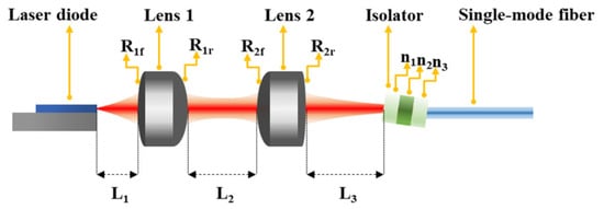
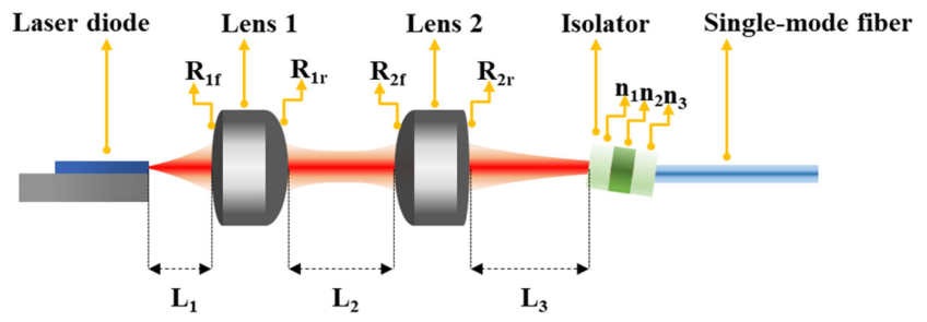
Figure 1 shows the free-space optical coupling architecture used in this study. The system was designed to represent a laser-to-fiber coupling path in a free-space optical transceiver module. The optical path consisted of a laser diode, Lens 1, Lens 2, an optical isolator, and a single-mode fiber. In this configuration, Lens 1 was used as the collimating lens to collect and reshape the divergent beam emitted from the laser diode, whereas Lens 2 was used as the coupling lens to focus the optical beam into the single-mode fiber after passing through the isolator. The axial positions and spacing among the optical components were regarded as critical assembly parameters because they directly influence the beam propagation, focusing condition, and final optical coupling efficiency. The laser diode was modeled with an asymmetric far-field divergence profile.
Figure 1.
Schematic configuration of the free-space laser-to-fiber coupling system.
The horizontal and vertical divergence angles were set to 32.7° and 42.1°, respectively. This asymmetric emission characteristic is important for laser-to-fiber coupling because the mode-field matching between the laser beam and the fiber mode strongly depends on both the beam divergence and the focused spot distribution [31]. These divergence angles were used as nominal input parameters to represent the asymmetric emission behavior of a high-speed telecom laser source rather than as experimentally measured values for the specific module investigated in this study. Therefore, the laser source model was included in the simulation to provide a realistic input condition for optical coupling optimization. The dual-lens structure was selected to improve the beam collimation and focusing process within the free-space coupling path [32,33]. Lens 1 had a thickness of 520 μm and a refractive index of 3.449. Lens 2 had a thickness of 500 μm and the same refractive index of 3.449. The refractive index was selected according to the optical properties of silicon at the operating wavelength, whereas the lens thicknesses were treated as nominal engineering dimensions representative of compact micro-optical components used in free-space optical packaging. The optical isolator was placed between the lens system and the fiber to represent the optical component commonly used in practical transceiver modules. The isolator consisted of three optical layers, in which the refractive indices of the first and third layers were 1.508 and the refractive index of the middle layer was 2.327. The thicknesses of the first and third layers were 200 μm, and the thickness of the middle layer was 320 μm. These values were used to construct a representative multilayer free-space isolator model consisting of cover-glass and Faraday-rotator regions. The specific refractive indices and layer thicknesses were treated as nominal simulation parameters reflecting representative material properties and practical component dimensions rather than values assigned to a single commercial isolator model. The output fiber was modeled as a single-mode fiber with a cladding refractive index of 1.447, a core refractive index of 1.452, a cladding diameter of 125 μm, a core diameter of 9 μm, and a numerical aperture of 0.12 [31]. The fiber geometry was selected to be consistent with standard telecom single-mode fiber characteristics, whereas the refractive-index and numerical-aperture values were adopted as nominal parameters for the present optical model. In particular, the 125 μm cladding diameter is consistent with ITU-T G.652-(characteristics of a single-mode optical fibre and cable. international telecommunication union: Geneva, Switzerland, 2024)-class single-mode fibers, while the remaining parameters define the baseline fiber model used in the simulation. Accordingly, the parameters used in this study include values informed by published references and commercial component specifications, together with nominal engineering assumptions introduced to define the baseline simulation model. Parameters not directly obtained from a published source or commercial datasheet should therefore be interpreted as simulation inputs rather than experimentally measured quantities. The detailed optical parameters used in the simulation are summarized in Table 1.
Table 1.
Optical component parameters used in the free-space laser-to-fiber coupling simulation.
2.2. Ray-Tracing Optical Simulation Model
The ray-tracing optical simulations were performed using LightTools 2024.03 (Synopsys, Inc., Sunnyvale, CA, USA). A ray-tracing optical simulation environment was established to evaluate the laser-to-fiber coupling performance under different lens assembly conditions [32,34]. The simulation model included the laser source, dual-lens optical system, isolator, and single-mode fiber. The optical coupling efficiency was calculated according to the optical power coupled into the single-mode fiber relative to the source power [10]. This efficiency was used as the main performance index for evaluating the lens assembly condition. In the simulation process, the axial positions and selected lens-related parameters were adjusted to search for high-efficiency optical coupling conditions [6,9,17,35]. For each set of assembly parameters, the optical beam propagation was calculated through the lens system and isolator, and the optical power coupled into the single-mode fiber was evaluated. The simulation result was then used as the feedback signal for the optimization algorithm. Through this procedure, the complex relationship between lens assembly parameters and optical coupling efficiency could be analyzed without relying on exhaustive manual tuning.
2.3. Simulation-Assisted Deep Reinforcement Learning Framework
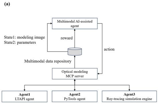
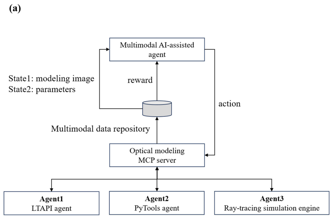
Figure 2 illustrates the simulation-assisted deep reinforcement learning workflow used for lens assembly optimization. As shown in Figure 2a, the proposed framework forms a closed-loop optimization process, in which the DRL agent updates the lens assembly parameters according to the reward feedback obtained from the ray-tracing optical simulation environment. In this framework, the optical simulation environment receives the lens assembly parameters from the agent, performs ray-tracing calculation, evaluates the optical coupling efficiency, and returns the corresponding reward to the agent. The agent then updates its policy according to the obtained reward and generates the next set of assembly parameters.
Figure 2.
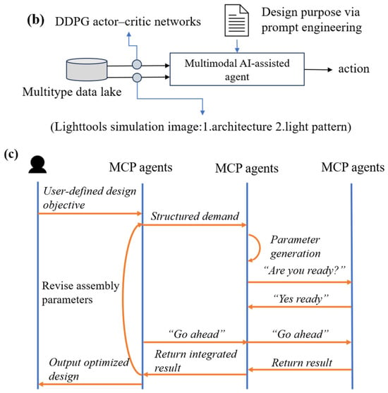
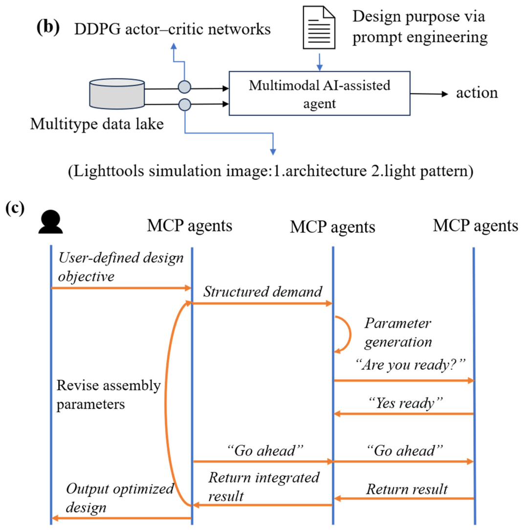
Overview of the simulation-assisted deep reinforcement learning framework. (a) Closed-loop optimization workflow for converting the design objective into structured lens assembly parameters and iteratively optimizing the optical coupling performance through ray-tracing simulation. (b) DDPG-based multimodal learning architecture using optical simulation images, light-pattern information, assembly parameters, and actor–critic networks. (c) Automated implementation flow integrating the AI-assisted agent, LTAPI/PyTools modules, MCP agents, and ray-tracing simulation engine for state, action, and reward exchange.
A deep deterministic policy gradient algorithm was employed in this study because the lens assembly optimization problem involves continuous design variables [30]. The DDPG algorithm is based on an actor–critic architecture [36,37]. The actor network determines the action used to modify the optical assembly parameters, whereas the critic network evaluates the expected reward associated with the current state and action [38]. Figure 2b further illustrates the learning architecture of the DDPG agent, where optical simulation information, light-pattern features, and assembly parameters are used as state information for actor–critic-based policy learning. This structure allows the agent to gradually learn an effective search policy in the continuous parameter space. For clarity and reproducibility, the main reinforcement learning formulation and training settings are summarized in Table 2. The learning rate was set to 5 × 10⁻⁵, the batch size was set to 4, and the maximum number of simulation runs per optimization episode was set to 200. These settings were used to train the DDPG agent through closed-loop interaction with the ray-tracing optical simulation environment.
Table 2.
Main reinforcement learning formulation and training settings.
2.4. Automated Modeling and Optimization Workflow
As shown in Figure 2c, an automated modeling and optimization workflow was established to improve the efficiency of data exchange between the optical simulation model and the DRL agent. The workflow included optical modeling, parameter update, ray-tracing calculation, performance evaluation, reward calculation, and policy update. The simulation images, optical patterns, and assembly parameters were treated as multimodal data sources for supporting the optimization process. The optimization process began with an initial optical model and a set of initial assembly parameters. After receiving the design objective, the agent generated an action to update the assembly condition. The ray-tracing simulation was then executed to calculate the optical response of the updated structure. The coupling efficiency was extracted and converted into a reward value. If the coupling performance was improved, the result was recorded and used to guide the next optimization step. If the result was not satisfactory, the agent revised the assembly parameters and repeated the simulation. This closed-loop process enabled automatic and iterative improvement of the lens assembly condition.
2.5. Reward Strategy Design
Based on the reward-feedback path shown in Figure 2a, different reward strategies were designed to investigate their influence on optimization behavior. Seven reward strategies were considered in this study: efficiency-only, balanced, and stability-oriented rewards. The efficiency-only reward was designed to directly maximize the optical coupling efficiency, whereas the balanced reward considered both coupling performance and local axial-perturbation stability to promote a more robust optical configuration [39,40]. The stability-oriented reward was introduced to examine whether the agent could avoid unstable or ineffective solutions during the search process. The reward strategy is an important factor in deep reinforcement learning because it determines the direction of policy update. If the reward only emphasizes a single objective, the agent may converge to a solution that is mathematically favorable but not physically meaningful for optical assembly. Therefore, different reward designs were compared to clarify their effects on convergence behavior, coupling performance, and solution stability. This analysis provides useful guidance for applying deep reinforcement learning to optical design automation and free-space optical transceiver packaging.
2.6. Reward Function Design
The reward function was designed to guide the reinforcement learning agent toward suitable lens assembly conditions. In this study, two optimization objectives were considered: optical coupling efficiency and local axial-perturbation stability. The optical coupling efficiency term was used to encourage the agent to search for high-efficiency laser-to-fiber coupling conditions, whereas the axial-sensitivity-related term was used to reduce the sensitivity of the optimized solution to small assembly deviations [39]. Accordingly, the total reward was constructed as a weighted combination of the coupling-efficiency-related reward and the assembly-stability-related reward, as
where is the total reward, is the coupling-efficiency-related reward, and is the assembly-stability-related reward. The weighting factors a and b determine the relative importance of coupling efficiency and local axial-perturbation stability, respectively. This metric evaluates only the local axial sensitivity of Lens 1 and Lens 2 and should not be interpreted as a complete manufacturing-tolerance or packaging-robustness metric. To quantitatively evaluate the local axial-perturbation stability, small positive and negative axial perturbations ranging from approximately ±2 μm were applied to the selected lens assembly parameters around each nominal configuration. During each perturbation, one selected assembly parameter was varied while the remaining parameters were kept unchanged. For a nominal configuration with a coupling efficiency of , the coupling efficiency was recalculated after each perturbation. The assembly-stability-related reward was evaluated according to the relative change in coupling efficiency and was expressed as
where is the coupling efficiency obtained after the i-th perturbation and N is the total number of perturbed configurations. The resulting axial-sensitivity score is dimensionless and has an upper bound of 1. The calculated value was not clipped to the interval [0, 1]. Therefore, negative values can occur when the mean relative variation in coupling efficiency exceeds unity. Such negative values were retained and interpreted as a penalty for configurations exhibiting high axial sensitivity. A value closer to 1 indicates a smaller variation in coupling efficiency under the applied axial perturbations. In this work, to examine the sensitivity of the DDPG optimization behavior to the reward weighting, seven weighting combinations satisfying (a + b = 1) were evaluated: ((a, b) = (1.0, 0.0)), ((0.8, 0.2)), ((0.6, 0.4)), ((0.5, 0.5)), ((0.4, 0.6)), ((0.2, 0.8)), and ((0.0, 1.0)). Here, (a) and (b) denote the contributions of the coupling-efficiency and assembly-stability terms, respectively. All other optical-model and DDPG settings were kept unchanged across the weighting conditions. This analysis was designed as a sensitivity assessment of the selected reward weights rather than as a formal multiobjective Pareto optimization.
2.7. Comparative Benchmark and Statistical Analysis
Five optimization methods were evaluated: deep deterministic policy gradient (DDPG), genetic algorithm (GA), particle swarm optimization (PSO), Bayesian optimization (BO), and randomized grid search. All methods used the same seven-dimensional parameter bounds and a common maximum budget of 20,000 optical-model evaluations per run. No method was terminated early; target attainment was evaluated retrospectively from the stored best-so-far efficiency histories. DDPG, GA, PSO, and BO were each evaluated using 10 independent random seeds. These four adaptive methods received the same seed-specific set of 40 scrambled-Sobol initial designs. Grid search used a fixed 5 × 7-point grid, of which 20,000 points were evaluated under each of 10 independently randomized traversal orders. Thus, the parameter bounds and evaluation budgets were identical, while the initialization procedures were kept consistent with the operating principle of each method. BO was included as a surrogate-based and sample-efficient baseline. It used an Extra-Trees ensemble to estimate the objective response and predictive uncertainty, followed by an expected-improvement acquisition criterion. Surrogate-assisted reinforcement learning was not included because it would introduce an additional approximation model whose training cost, predictive error, and out-of-distribution behavior would require separate validation. An independent model-specific reference efficiency was obtained using 131,072 scrambled-Sobol samples followed by Powell refinement from the 12 best Sobol candidates, with a maximum of 600 local evaluations per start. This procedure produced ηREF = 20.854%. The value is used as a reproducible numerical reference for the specified optical model and parameter bounds and is not claimed to be a mathematically proven global optimum. The primary high-efficiency target was defined as ηtarget = 0.95ηREF = 19.811%. Sensitivity analyses were additionally performed at 0.90ηREF and 0.99ηREF. For each run, the evaluations-to-target value was calculated as the first evaluation n satisfying
Runs that did not attain a target within the common budget were retained in the success-rate calculation and assigned the full budget of 20,000 evaluations for the budget-penalized time-to-target statistic. The convergence curves are reported as the mean best-so-far efficiency ± one standard deviation across 10 independent runs. Evaluations to target are reported as mean ± standard deviation, bootstrap 95% confidence interval, median, interquartile range, and success rate. Overall differences among the five methods were evaluated using the Friedman test. Post hoc pairwise comparisons used two-sided Wilcoxon signed-rank tests with Holm correction for multiple comparisons.
2.8. Correlation Analysis
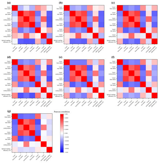
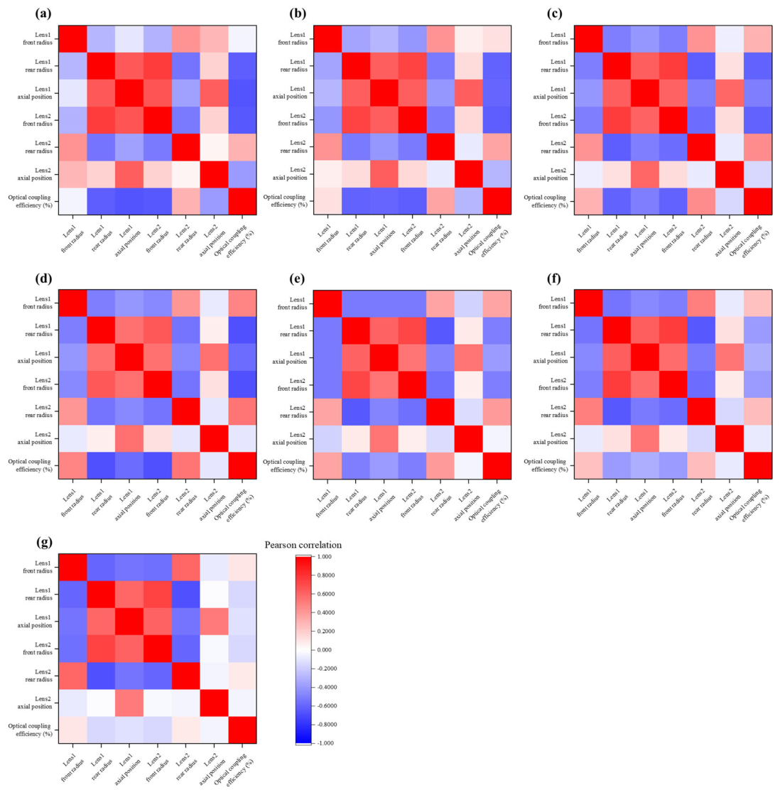
For each reward-weighting condition, Pearson correlation coefficients were calculated separately between the six optical design parameters and coupling efficiency using the samples recorded during the DDPG optimization process. The coefficients range from −1 to +1, where the sign indicates the direction of the linear association and the absolute value indicates its magnitude. Because consecutive evaluations within an optimization trajectory are not statistically independent, the coefficients were used to describe the sampled search behavior and were not subjected to independent-sample significance testing or interpreted as causal relationships.
3. Results
3.1. Convergence and Target-Attainment Performance
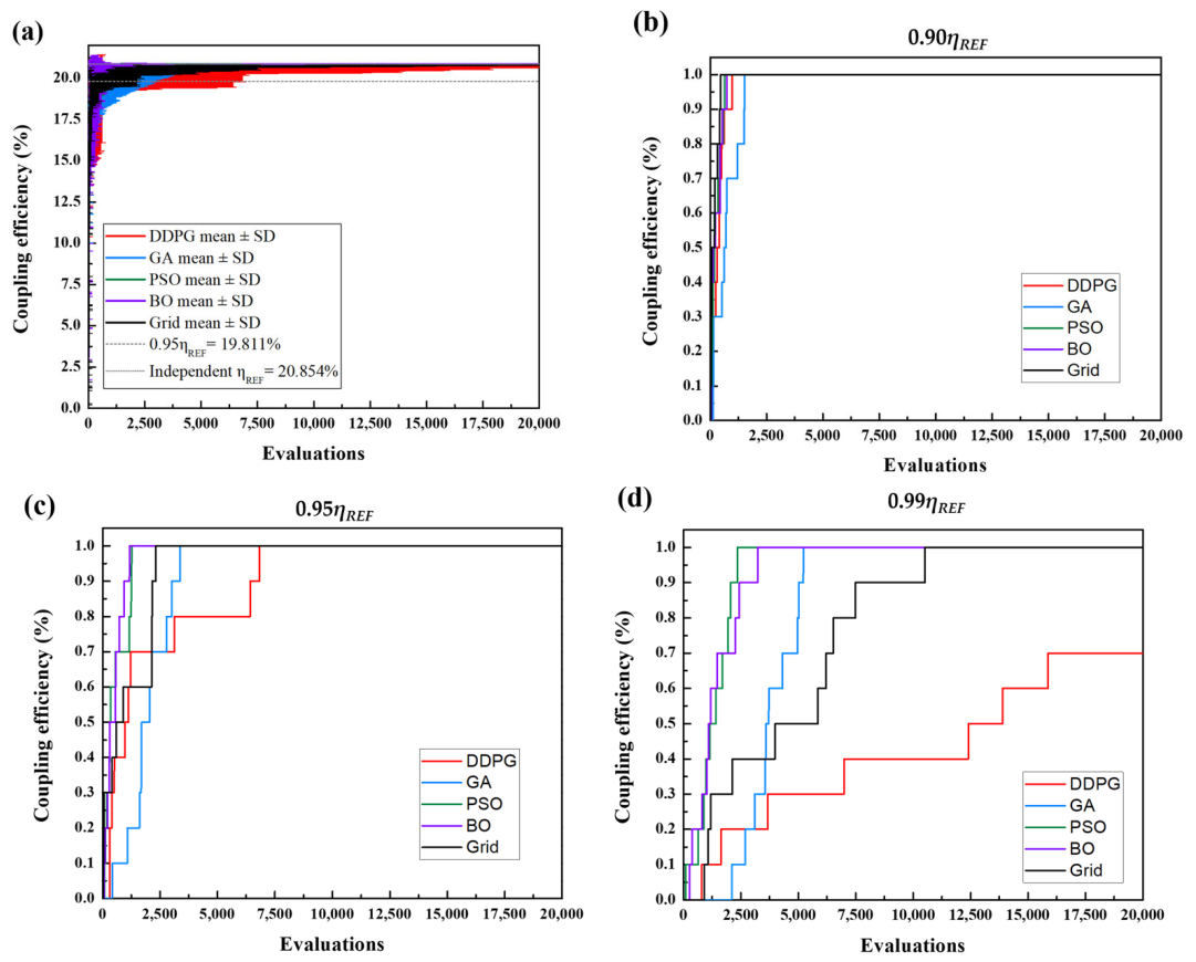
Figure 3 compares the convergence and target-attainment performance of five optimization methods for lens assembly optimization, including deep deterministic policy gradient (DDPG), genetic algorithm (GA) [41,42], particle swarm optimization (PSO) [43,44], Bayesian optimization (BO) [45], and randomized grid search. All methods were evaluated under the same budget of 20,000 optical-model evaluations. Figure 3a shows the mean best-so-far coupling efficiency obtained from 10 independent runs, and the shaded regions represent ±1 standard deviation. The horizontal reference lines indicate the independently determined reference efficiency, ηREF = 20.854%, and the primary target, 0.95ηREF = 19.811%. Figure 3b–d shows the fractions of runs attaining 0.90ηREF, 0.95ηREF, and 0.99ηREF, respectively. Table 3 summarizes the quantitative performance of the five optimization methods. After 20,000 evaluations, the final mean coupling efficiencies were 20.747 ± 0.129% for DDPG, 20.853 ± 0.00003% for GA, 20.854 ± 0% for PSO, 20.853 ± 0.00033% for BO, and 20.804 ± 0.0352% for randomized grid search. These values correspond to 99.488%, 99.9999%, approximately 100%, 99.9980%, and 99.762% of ηREF, respectively. For the primary target of 0.95ηREF, BO required the fewest evaluations on average, with 495.2 ± 366.2 evaluations, followed by PSO with 557.9 ± 478.9, randomized grid search with 1079.2 ± 992.0, GA with 1982.3 ± 894.9, and DDPG with 2122.7 ± 2515.4. All five methods successfully attained this target in all 10 runs. The corresponding median, interquartile range, and bootstrap 95% confidence interval are also summarized in Table 3. The relative performance of the optimization methods depended on the selected target level. At 0.90ηREF, randomized grid search required the lowest mean number of evaluations. At the more stringent 0.99ηREF target, PSO and BO required 1318.8 ± 701.7 and 1414.0 ± 948.4 evaluations, respectively, and both methods attained the target in all runs. In comparison, DDPG attained the 0.99ηREF target in 7 of 10 runs, with a budget-penalized mean of 11,527.3 ± 7717.3 evaluations. For the primary 0.95ηREF target, the Friedman test showed an overall difference among the five methods (χ2(4) = 15.44, p = 0.0039). The Holm-corrected pairwise Wilcoxon signed-rank tests showed that GA required significantly more evaluations than PSO and BO, with an adjusted p-value of 0.0195 for both comparisons. The remaining pairwise comparisons did not show statistically significant differences after correction. These results indicate that the optimization performance depends on the required target level, and no single method showed superior performance under all evaluated conditions.
Figure 3.
Convergence and target-attainment performance of the five optimization methods under a common 20,000-evaluation budget. (a) Mean best-so-far coupling efficiency over 10 independent runs with ±1 standard deviation. The horizontal lines indicate the reference efficiency ηREF = 20.854% and the primary target 0.95ηREF = 19.811%. (b–d) Fractions of runs attaining 0.90ηREF, 0.95ηREF, and 0.99ηREF, respectively.
Table 3.
Final coupling efficiency and target-attainment statistics of the five optimization methods under the common 20,000-evaluation benchmark.
3.2. Effect of Reward Weighting on Optimization Behavior
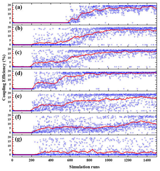
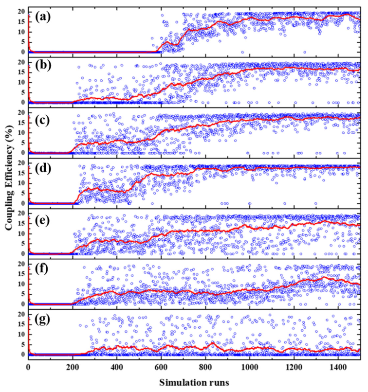
Figure 4 compares the coupling-efficiency trajectories obtained by the DDPG optimizer under seven reward-weighting conditions. The efficiency-only condition (a = 1.0, b = 0.0) reached a high-efficiency region during the later stage of optimization. The intermediate conditions with relatively high efficiency weights, including (a = 0.8, b = 0.2) and (a = 0.6, b = 0.4), also achieved high coupling-efficiency levels. Among the representative trajectories, the (a = 0.6, b = 0.4) condition showed a comparatively high and more concentrated efficiency distribution during the later optimization stage. The equal-weight condition (a = 0.5, b = 0.5) maintained a relatively high coupling-efficiency level but did not show a uniquely superior behavior compared with the other intermediate weighting conditions. As the efficiency weight was further reduced, the coupling-efficiency level generally decreased. This trend was more evident for (a = 0.2, b = 0.8) and (a = 0.0, b = 1.0), where the trajectories remained substantially below those obtained with larger efficiency weights. These results indicate that the sampled coupling-efficiency behavior is sensitive to the reward weighting. However, Figure 4 presents representative sequential trajectories rather than results from repeated independent runs. Therefore, the figure is used to illustrate the influence of reward weighting on the optimization behavior and is not used to establish the statistical superiority of any individual weighting condition.
Figure 4.
Coupling-efficiency samples and moving-average trajectories obtained during representative DDPG optimization runs under seven reward-weighting conditions: (a) (a = 1.0, b = 0.0); (b) (a = 0.8, b = 0.2); (c) (a = 0.6, b = 0.4); (d) (a = 0.5, b = 0.5); (e) (a = 0.4, b = 0.6); (f) (a = 0.2, b = 0.8); and (g) (a = 0.0, b = 1.0). The blue symbols represent the sequentially evaluated coupling efficiencies, and the red curves represent the corresponding moving averages.
3.3. Distribution of Coupling Efficiency Samples Under Different DDPG Reward-Weighting Conditions
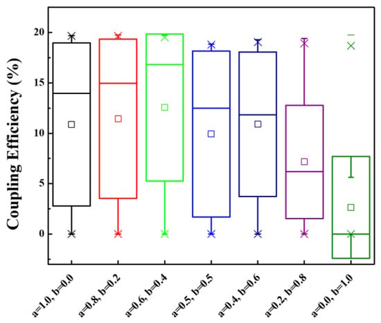
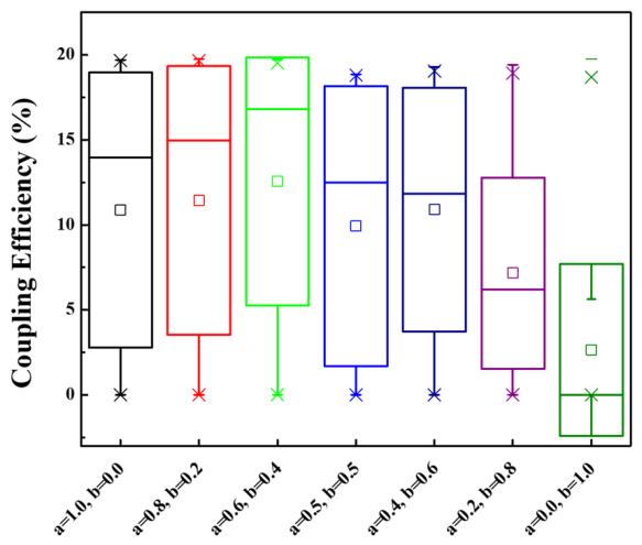
Figure 5 summarizes the coupling-efficiency distributions obtained from representative DDPG trajectories under seven reward-weighting conditions. The (a = 0.6, b = 0.4) setting exhibited the highest median coupling efficiency among the displayed distributions, followed by the cases with relatively large efficiency weights. The equal-weight setting (a = 0.5, b = 0.5) maintained a relatively high efficiency range, but its median was lower than that of (a = 0.6, b = 0.4). As the stability-related weight increased, the coupling-efficiency distributions generally shifted toward lower values. This trend was more evident for (a = 0.2, b = 0.8), which showed a substantially lower median efficiency, while the stability-only setting (a = 0.0, b = 1.0) produced a distribution concentrated mainly in the low-efficiency region. The additional intermediate weighting conditions indicate that (a = 0.5, b = 0.5) does not show a uniquely superior coupling-efficiency distribution within the investigated range. Therefore, it is treated as a symmetric equal-weight reference representing one selected trade-off between coupling efficiency and local axial-perturbation stability. Because the samples within each distribution were collected sequentially from a representative optimization trajectory and are temporally correlated, the boxplots are used for descriptive comparison and are not interpreted as independent-run statistical evidence.
Figure 5.
Coupling-efficiency distributions under seven reward-weighting conditions. Each box summarizes 1500 sequential evaluations from a representative DDPG trajectory. The center line, box boundaries, and open square indicate the median, interquartile range, and mean, respectively.
3.4. Distribution of Reward Samples Under Different DDPG Reward-Weighting Conditions
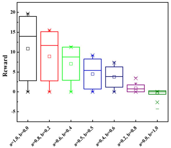
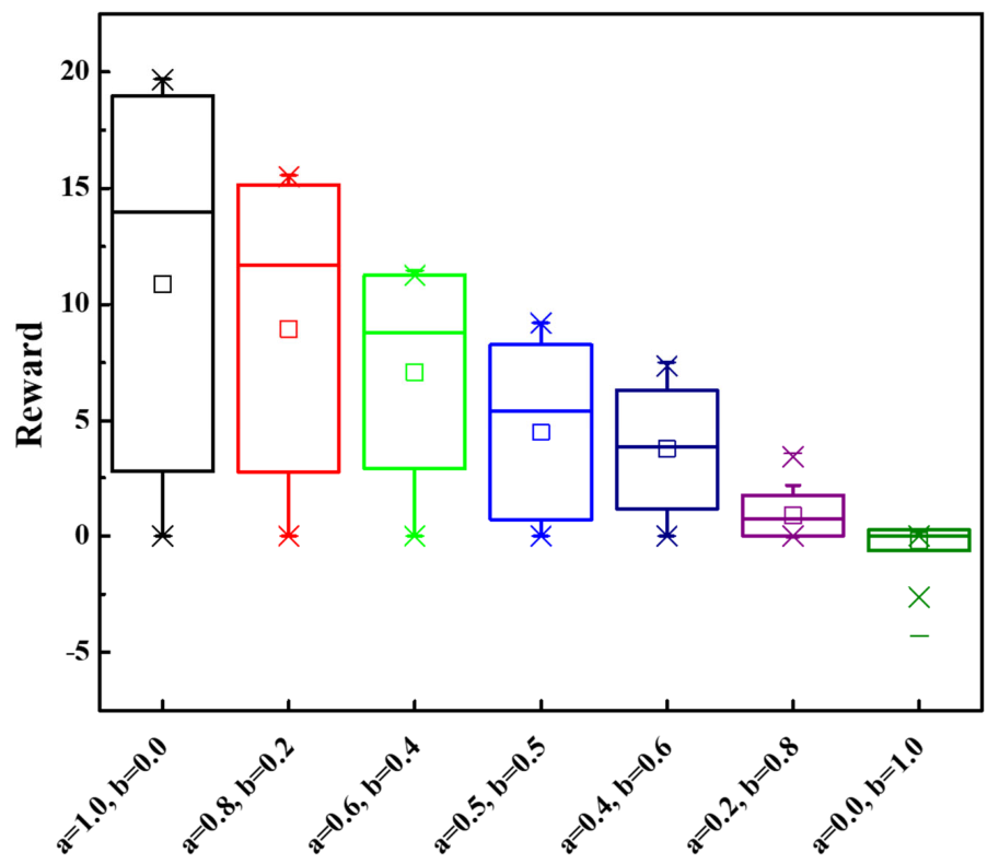
Figure 6 presents the reward-value distributions obtained from representative DDPG optimization trajectories under seven reward-weighting conditions. Each distribution contains 1500 sequential reward samples from the corresponding trajectory. As the efficiency-related weight decreased, the reward distributions generally shifted toward lower values. The efficiency-only condition (a = 1.0, b = 0.0) showed the highest median and upper reward range, whereas the intermediate weighting conditions exhibited progressively lower reward levels. The equal-weight condition (a = 0.5, b = 0.5) remained mainly in the positive reward region. When the stability-related contribution became dominant, particularly for (a = 0.2, b = 0.8) and (a = 0.0, b = 1.0), the reward distributions were concentrated near zero, and negative values were also observed for the stability-only condition. Because the seven weighting conditions use different combinations of the efficiency-related and stability-related reward terms, their absolute reward values should not be directly interpreted as a common performance metric. Therefore, Figure 6 is used to illustrate the change in reward behavior with different weighting conditions rather than to rank their optimization performance. In addition, the samples were sequentially collected from representative optimization trajectories and are temporally correlated; therefore, they are not treated as statistically independent observations.
Figure 6.
Reward-value distributions under seven reward-weighting conditions. Each box summarizes 1500 sequential reward samples from a representative DDPG trajectory. The center line and box boundaries indicate the median and interquartile range, respectively, and the open square denotes the mean.
3.5. Relationship Between Reward Value and Coupling Efficiency
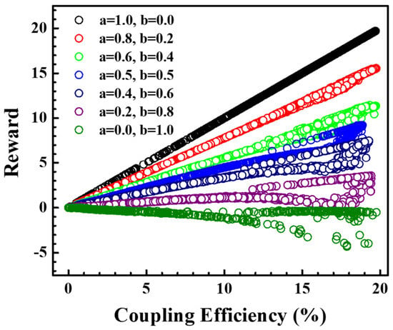
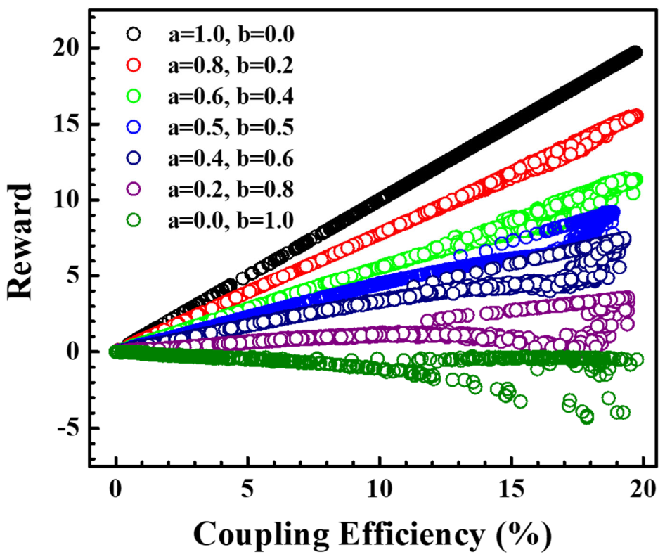
Figure 7 shows the relationship between coupling efficiency and the reward obtained from representative DDPG optimization trajectories under seven reward-weighting conditions. For the efficiency-only condition (a = 1.0, b = 0.0), the reward increased almost linearly with coupling efficiency because only the efficiency-related term contributed to the reward function. As the efficiency weight a decreased, the dependence of reward on coupling efficiency became weaker, while a larger spread of reward values appeared at similar efficiency levels due to the increasing contribution of the stability-related term. For the stability-only condition (a = 0.0, b = 1.0), coupling efficiency was not directly included in the reward function, and no clear monotonic relationship between reward and coupling efficiency was observed. The intermediate weighting conditions showed a gradual transition between these two limiting cases. These results illustrate how the relative contributions of the efficiency- and stability-related terms affect the reward–efficiency relationship. However, because each weighting condition represents a different mathematical composition of the reward function, the absolute reward values and apparent slopes should not be directly compared as a common measure of optimization performance. Therefore, Figure 7 is used to describe the influence of reward weighting on the optimization behavior and is not used to identify an optimal weighting condition.
Figure 7.
Reward–efficiency relationship under seven reward-weighting conditions obtained from representative DDPG optimization trajectories.
3.6. Correlation Analysis of the DDPG Sampled Design Parameters and Coupling Efficiency
Figure 8 presents the Pearson correlation heatmaps of six optical design parameters and coupling efficiency obtained from representative DDPG optimization trajectories under seven reward-weighting conditions. Figure 8a–g correspond to (a, b) = (1.0, 0.0), (0.8, 0.2), (0.6, 0.4), (0.5, 0.5), (0.4, 0.6), (0.2, 0.8), and (0.0, 1.0), respectively. Reward was not included as an explicit variable; therefore, the heatmaps describe parameter–parameter and parameter–efficiency associations within the sampled optimization trajectories. Under the efficiency-only condition in Figure 8a, the Lens 1 axial position showed the largest absolute correlation with coupling efficiency (r ≈ 0.66). The Lens 1 rear radius and Lens 2 front radius also exhibited relatively strong negative correlations, both approximately (r = −0.62). In contrast, the Lens 1 front radius showed only a weak association with coupling efficiency. The Lens 2 rear radius and Lens 2 axial position exhibited positive and negative correlations of approximately (r = 0.29) and (r = −0.37), respectively. For the intermediate weighting conditions, the Lens 1 rear radius and Lens 2 front radius remained the most consistently negative efficiency-associated parameters. The Lens 1 axial position also generally showed a negative correlation, whereas the Lens 2 rear radius exhibited a positive correlation. Under the equal-weight condition (a = 0.5, b = 0.5), the Lens 1 rear radius and Lens 2 front radius showed correlations of approximately (r = −0.67) and (r = −0.66), respectively, while the Lens 2 rear radius showed the strongest positive correlation (r ≈ 0.55). The Lens 2 axial position showed only a weak association with coupling efficiency. As the stability-related contribution increased, the magnitudes of the parameter–efficiency correlations generally decreased. Under the stability-only condition (a = 0.0, b = 1.0), all six design parameters showed weak correlations with coupling efficiency, with absolute coefficients of approximately 0.15 or less. This result indicates that the sampled parameter–efficiency structure becomes less pronounced when coupling efficiency is no longer directly included in the reward function. Overall, the Lens 1 rear radius and Lens 2 front radius were the most consistently negative efficiency-associated parameters, whereas the Lens 2 rear radius generally showed a positive association. The Lens 2 axial position was among the weakest efficiency-associated parameters under most mixed-weight and stability-dominant conditions. These results indicate that the sampled parameter–efficiency relationships vary with the reward formulation used during DDPG optimization. It should be noted that these Pearson coefficients describe pairwise linear associations within representative sequential optimization trajectories. They do not indicate causal relationships and do not account for possible interactions among multiple optical parameters. In addition, because reward was not included as a variable in the correlation analysis, differences among the heatmaps should not be interpreted as direct evidence of a reward–efficiency correlation.
Figure 8.
Pearson correlation heatmaps of optical design parameters and coupling efficiency under seven reward-weighting conditions: (a–g) (a, b) = (1.0, 0.0), (0.8, 0.2), (0.6, 0.4), (0.5, 0.5), (0.4, 0.6), (0.2, 0.8), and (0.0, 1.0), respectively.
4. Discussion
The common benchmark demonstrates that all five optimization methods can identify lens configurations with coupling efficiencies close to the independently determined numerical reference, although their sample efficiencies depend on the selected target level. Randomized grid search reached the relatively permissive 0.90ηREF target with the lowest mean number of optical-model evaluations. In contrast, BO and PSO required fewer evaluations to reach the more stringent 0.95ηREF and 0.99ηREF targets. This target-dependent behavior suggests that locating a broadly acceptable region is relatively straightforward for the present multidimensional optical model, whereas approaching the high-efficiency reference region benefits from a more adaptive search strategy. DDPG achieved a final mean coupling efficiency corresponding to approximately 99.49% of ηREF and reached the 0.95ηREF target in all independent runs. However, DDPG required more optical-model evaluations and showed greater run-to-run variability than BO and PSO. Therefore, the present results do not support a general conclusion that DDPG is the most sample-efficient method for the static and deterministic optimization problem considered in this study. BO and PSO appear more suitable when the main objective is to minimize the number of optical-model evaluations required to approach the numerical reference. The potential value of DDPG instead lies in its policy-based formulation, which may provide advantages for problems involving state-dependent observations, sequential assembly decisions, time-varying disturbances, or online control. Because these capabilities were not examined in the present benchmark, they should be regarded as possible directions for future investigation rather than as demonstrated advantages of the proposed framework.
The expanded reward-weighting analysis further clarifies the influence of the reward formulation on the DDPG optimization behavior. The original seven weighting conditions were extended to seven conditions while maintaining a + b = 1. Among the representative trajectories, the (a = 0.6, b = 0.4) condition exhibited the highest median coupling efficiency, whereas conditions with larger stability-related contributions generally showed lower coupling-efficiency distributions. The equal-weight condition (a = 0.5, b = 0.5) maintained a relatively high efficiency level but did not show a uniquely superior result compared with the other intermediate weighting conditions. These results indicate that a sufficiently large contribution from the efficiency-related reward term is necessary to guide the DDPG agent toward high-coupling-efficiency configurations. However, the present results do not demonstrate that (a = 0.6, b = 0.4), (a = 0.5, b = 0.5), or any other investigated weighting condition represents an optimal engineering trade-off. First, the samples shown in Figure 4, Figure 5, Figure 6 and Figure 7 were collected sequentially from representative optimization trajectories and are therefore temporally correlated rather than statistically independent. Second, the stability-related term included in the reward function is an optimization metric and is not equivalent to a separately validated engineering robustness or tolerance metric. Third, the absolute reward values cannot be directly compared across different weighting conditions because the mathematical composition of the reward function changes with a and b. Therefore, the equal-weight condition is retained only as a symmetric reference condition for discussing the influence of reward composition. A more rigorous determination of the axial-sensitivity-related term would require repeated independent runs, separately reported coupling-efficiency and stability metrics, and a multiobjective or Pareto-type analysis.
The reward–efficiency relationship shown in Figure 7 also reflects the mathematical composition of the reward function. Under the efficiency-only condition, the reward increased almost linearly with coupling efficiency because the efficiency-related term was the sole contribution to the reward. As the efficiency weight decreased, the dependence of reward on coupling efficiency became weaker, while the spread of reward values at similar efficiency levels increased because of the increasing contribution from the stability-related term. Under the stability-only condition, coupling efficiency was not directly included in the reward function, and no clear monotonic relationship between reward and coupling efficiency was observed. Therefore, the absolute reward values and apparent slopes in Figure 7 should not be interpreted as a common measure for ranking the optimization performance of different weighting conditions. The differences among the correlation patterns in Figure 8 may reflect the different regions of the parameter space sampled by the DDPG agent under different reward formulations. The reward function determines the feedback used for policy updating and may consequently influence the search trajectory and the combinations of optical parameters visited by the agent. Under the efficiency-dominant and mixed-weight conditions, the Lens 1 rear radius and Lens 2 front radius were among the parameters showing the most consistent negative associations with coupling efficiency, whereas the Lens 2 rear radius generally showed a positive association. As the stability-related contribution increased, the magnitudes of the parameter–efficiency correlations generally became weaker. Under the stability-only condition, all six design parameters showed only weak correlations with coupling efficiency.
From an optical perspective, these parameter–efficiency associations are consistent with the sensitivity of laser-to-fiber coupling to lens geometry, axial spacing, beam focusing, and mode-field matching. Changes in lens curvature and axial positions can modify the focused beam radius, beam-waist location, and focal condition at the fiber input plane. A mismatch between the focused beam profile and the fundamental fiber mode can reduce the mode-field overlap and decrease the coupling efficiency. However, the Pearson coefficients in Figure 8 represent pairwise linear associations within the parameter combinations sampled during the optimization trajectories. They do not isolate the independent physical contribution of each design parameter and do not establish causal relationships. Interactions among multiple lens and assembly parameters, together with the nonuniform sampling produced by the optimizer, may also contribute to the observed correlation patterns. In addition, reward was not included as an explicit variable in the correlation analysis; therefore, differences among the heatmaps should not be interpreted as direct evidence of a reward–efficiency correlation. Several limitations should be considered when interpreting these results. First, the present study is based entirely on ray-tracing simulation and should therefore be regarded as a simulation-based proof of concept for lens assembly optimization rather than as a fully validated optical packaging solution. The optimized configurations represent the performance obtained under the assumed nominal optical model. It should be emphasized that the stability-related metric used in the present work considers only local axial perturbations and does not constitute a complete manufacturing-tolerance or production-yield analysis. Manufacturing tolerances, positioning resolution, surface-form errors, refractive-index variations, lens decenter, tilt, and axial placement errors may reduce the coupling efficiency achievable in an actual optical package. Therefore, the numerical precision of the optimized parameters should not be interpreted as the required or achievable engineering precision. A tolerance-aware assessment using experimentally qualified parameter ranges and Monte Carlo sampling, together with experimental or hardware-level validation, will be required to determine the achievable coupling-efficiency distribution and practical applicability of the optimized configurations. Second, the independently determined reference efficiency used in this study is a high-budget numerical reference rather than a mathematically proven global optimum. Comparisons with ηREF should therefore be interpreted as comparisons with a reproducible numerical reference obtained within the investigated parameter bounds. Third, although the comparative benchmark included repeated independent runs, the reward-weighting analysis was performed using representative sequential trajectories and therefore does not provide statistical evidence of differences in engineering robustness among the weighting conditions. Finally, the present benchmark considered a static and deterministic optical objective and did not include time-dependent disturbances, sequential assembly actions, or online adaptation.
Future work will therefore focus on experimentally qualified tolerance models, Monte Carlo yield analysis, repeated independent evaluation of intermediate reward weights, and hardware-level validation. In addition, policy-based reinforcement learning and surrogate-assisted optimization may be further investigated for adaptive or online optical assembly applications, provided that surrogate-training cost, prediction uncertainty, and out-of-distribution errors are separately evaluated from the optical-model evaluation budget.
5. Conclusions
In this study, a simulation-assisted DRL framework was developed for lens assembly optimization in a free-space optical transceiver module and compared with GA, PSO, BO, and randomized grid search under a common evaluation protocol. All five methods obtained final solutions close to the numerical reference efficiency of 20.854%. DDPG achieved a final mean coupling efficiency of 20.747 ± 0.1287%, corresponding to 99.49% of ηREF, and reached the 0.95ηREF target in all 10 independent runs. However, BO and PSO required fewer optical-model evaluations to reach the higher-efficiency targets, indicating that the relative performance depends on the required solution quality and available evaluation budget. The expanded reward-weighting analysis showed that the coupling-efficiency behavior was strongly influenced by the relative contributions of the efficiency- and stability-related reward terms. Among the representative trajectories, the (a = 0.6, b = 0.4) condition exhibited the highest median coupling efficiency, whereas the equal-weight condition (a = 0.5, b = 0.5) maintained a relatively high efficiency level and served as a symmetric reference for evaluating the trade-off between coupling efficiency and the local axial-sensitivity metric. However, neither condition can be regarded as a demonstrated optimum from the present analysis. Because the present study is based on ray-tracing simulation, further validation is required before practical implementation. Future work will include experimentally qualified tolerance models, Monte Carlo yield analysis, repeated independent evaluation of different reward-weighting conditions, and hardware-level validation.
Author Contributions
Conceptualization, C.-F.K. and C.-H.C.; data curation, C.-C.H. and H.-J.L.; formal analysis, C.-C.H.; investigation, C.-H.H. and C.-H.C.; methodology, T.-C.K., Y.E.D., T.-Y.L. and C.-W.S.; writing—original draft preparation, C.-H.C.; resources, H.-C.K. All authors have read and agreed to the published version of the manuscript.
Funding
This work was supported by the National Science and Technology Council (NSTC), Taiwan (NSTC 114-2222-E-033-002-MY3, NSTC 114-2637-E-033-005 and NSTC 115-2221-E-033-050). The study by Yu. E. Drobotov was carried out with the financial support of the Southern Federal University, scientific project No. VnGr/26-01-MM.
Data Availability Statement
The original contributions presented in this study are included in the article. Further inquiries can be directed to the corresponding author.
Conflicts of Interest
Chih-Chang Hung is employed by Bolite Co., Ltd., and Che-Hsuan Huang is employed by LEDA Creative Technology Ltd. The remaining authors declare that the research was conducted in the absence of any commercial or financial relationships that could be construed as a potential conflict of interest.
Abbreviations
The following abbreviations are used in this manuscript:
| DRL | Deep reinforcement learning |
| AI | Artificial intelligence |
| DDPG | Deep deterministic policy gradient |
| GA | Genetic algorithm |
| PSO | Particle swarm optimization |
| BO | Bayesian optimization |
| IQR | Interquartile range |
| CI | Confidence interval |
References
- Agrell, E.; Karlsson, M.; Chraplyvy, A.R.; Richardson, D.J.; Krummrich, P.M.; Winzer, P.; Roberts, K.; Fischer, J.K.; Savory, S.J.; Eggleton, B.J.; et al. Roadmap of optical communications. J. Opt. 2016, 18, 063002. [Google Scholar] [CrossRef] [Scilit]
- Winzer, P.J.; Neilson, D.T. From scaling disparities to integrated parallelism: A decathlon for a decade. J. Light. Technol. 2017, 35, 1099–1115. [Google Scholar] [CrossRef] [Scilit]
- Miller, D.A.B. Device requirements for optical interconnects to silicon chips. Proc. IEEE 2009, 97, 1166–1185. [Google Scholar] [CrossRef] [Scilit]
- Cheng, Q.; Bahadori, M.; Glick, M.; Rumley, S.; Bergman, K. Recent advances in optical technologies for data centers: A review. Optica 2018, 5, 1354–1370. [Google Scholar] [CrossRef] [Scilit]
- Zhou, H.; Xu, H.; Duan, J.-A. Review of the technology of a single mode fiber coupling to a laser diode. Opt. Fiber Technol. 2020, 55, 102097. [Google Scholar] [CrossRef] [Scilit]
- Kawano, K. Coupling characteristics of lens systems for laser diode modules using single-mode fiber. Appl. Opt. 1986, 25, 2600–2605. [Google Scholar] [CrossRef] [Scilit]
- Fadhali, M.; Zainal, J.; Munajat, Y.; Ali, J.; Abdul Rahman, R. Efficient coupling and relaxed alignment tolerances in pigtailing of a laser diode using dual ball lenses. Optik 2009, 120, 384–389. [Google Scholar] [CrossRef] [Scilit]
- Wang, L.A.; Su, C.D. Tolerance analysis of aligning an astigmatic laser diode with a single-mode optical fiber. J. Light. Technol. 1996, 14, 2757–2762. [Google Scholar] [CrossRef]
- Zhong, S.; Xu, C.; Duan, L.; Zhang, F.; Duan, J. Optimizing the efficiency of a laser diode and single-mode fiber coupling using multi-aspherical lenses. Opt. Fiber Technol. 2022, 68, 102781. [Google Scholar] [CrossRef] [Scilit]
- Wagner, R.E.; Tomlinson, W.J. Coupling efficiency of optics in single-mode fiber components. Appl. Opt. 1982, 21, 2671–2688. [Google Scholar] [CrossRef] [Scilit]
- Ratowsky, R.P.; Yang, L.; Deri, R.J.; Chang, K.W.; Kallman, J.S.; Trott, G. Laser diode to single-mode fiber ball lens coupling efficiency: Full-wave calculation and measurements. Appl. Opt. 1997, 36, 3435–3438. [Google Scholar] [CrossRef] [Scilit]
- Gangopadhyay, S.; Sarkar, S. ABCD matrix for reflection and refraction of Gaussian light beams at surfaces of hyperboloid of revolution and efficiency computation for laser diode to single-mode fiber coupling by way of a hyperbolic lens on the fiber tip. Appl. Opt. 1997, 36, 8582–8586. [Google Scholar] [CrossRef] [Scilit]
- Zhang, D.; Kong, J.; Zhu, L.; Wu, X.; Liu, S.; Ma, X. Theoretical investigation on the effective coupling optical system between an astigmatic tapered diode laser beam and single-mode optical fibers. Appl. Opt. 2024, 63, 6065–6072. [Google Scholar] [CrossRef] [Scilit]
- Gangopadhyay, S.; Sarkar, S.N. Laser diode to single-mode fibre excitation via hyperbolic lens on the fibre tip: Formulation of ABCD matrix and efficiency computation. Opt. Commun. 1996, 132, 55–60. [Google Scholar] [CrossRef] [Scilit]
- Das, B.; Maiti, A.K.; Gangopadhyay, S. Laser diode to single-mode circular core dispersion-shifted/dispersion-flattened fiber excitation via hyperbolic microlens on the fiber tip: Prediction of coupling efficiency by ABCD matrix formalism. Optik 2014, 125, 3277–3282. [Google Scholar] [CrossRef] [Scilit]
- Hillerich, B. Shape analysis and coupling loss of microlenses on single-mode fiber tips. Appl. Opt. 1988, 27, 3102–3106. [Google Scholar] [CrossRef] [Scilit]
- Wilson, R.G. Ball-lens coupling efficiency for laser-diode to single-mode fiber: Comparison of independent studies by distinct methods. Appl. Opt. 1998, 37, 3201–3205. [Google Scholar] [CrossRef] [Scilit]
- Campbell, S.D.; Sell, D.; Jenkins, R.P.; Whiting, E.B.; Fan, J.A.; Werner, D.H. Review of numerical optimization techniques for meta-device design. Opt. Mater. Express 2019, 9, 1842–1863. [Google Scholar] [CrossRef] [Scilit]
- Karanov, B.; Chagnon, M.; Thouin, F.; Eriksson, T.A.; Bülow, H.; Lavery, D.; Bayvel, P.; Schmalen, L. End-to-end deep learning of optical fiber communications. J. Light. Technol. 2018, 36, 4843–4855. [Google Scholar] [CrossRef] [Scilit]
- Malkiel, I.; Mrejen, M.; Nagler, A.; Arieli, U.; Wolf, L.; Suchowski, H. Plasmonic nanostructure design and characterization via deep learning. Light. Sci. Appl. 2018, 7, 60. [Google Scholar] [CrossRef] [Scilit]
- Peurifoy, J.; Shen, Y.; Jing, L.; Yang, Y.; Cano-Renteria, F.; DeLacy, B.G.; Joannopoulos, J.D.; Tegmark, M.; Soljačić, M. Nanophotonic particle simulation and inverse design using artificial neural networks. Sci. Adv. 2018, 4, eaar4206. [Google Scholar] [CrossRef] [Scilit]
- Liu, D.; Tan, Y.; Khoram, E.; Yu, Z. Training deep neural networks for the inverse design of nanophotonic structures. ACS Photonics 2018, 5, 1365–1369. [Google Scholar] [CrossRef] [Scilit]
- Musumeci, F.; Rottondi, C.; Nag, A.; Macaluso, I.; Zibar, D.; Ruffini, M.; Tornatore, M. An overview on application of machine learning techniques in optical networks. IEEE Commun. Surv. Tutor. 2019, 21, 1383–1408. [Google Scholar] [CrossRef] [Scilit]
- So, S.; Rho, J. Designing nanophotonic structures using conditional deep convolutional generative adversarial networks. Nanophotonics 2019, 8, 1255–1261. [Google Scholar] [CrossRef] [Scilit]
- Wiecha, P.R.; Muskens, O.L. Deep learning meets nanophotonics: A generalized accurate predictor for near fields and far fields of arbitrary 3D nanostructures. Nano Lett. 2020, 20, 329–338. [Google Scholar] [CrossRef] [Scilit]
- Dinsdale, N.J.; Wiecha, P.R.; Delaney, M.; Reynolds, J.; Ebert, M.; Zeimpekis, I.; Thomson, D.J.; Reed, G.T.; Lalanne, P.; Vynck, K.; et al. Deep learning enabled design of complex transmission matrices for universal optical components. ACS Photonics 2021, 8, 283–295. [Google Scholar] [CrossRef] [Scilit]
- Tseng, E.; Colburn, S.; Whitehead, J.; Huang, L.; Baek, S.H.; Majumdar, A.; Heide, F. Neural nano-optics for high-quality thin lens imaging. Nat. Commun. 2021, 12, 6493. [Google Scholar] [CrossRef] [Scilit]
- Sun, C.; Kaiser, E.; Brunton, S.L.; Kutz, J.N. Deep reinforcement learning for optical systems: A case study of mode-locked lasers. Mach. Learn. Sci. Technol. 2020, 1, 045013. [Google Scholar] [CrossRef] [Scilit]
- Li, R.; Zhang, C.; Xie, W.; Gong, Y.; Ding, F.; Dai, H.; Chen, Z.; Yin, F.; Zhang, Z. Deep reinforcement learning empowers automated inverse design and optimization of photonic crystals for nanoscale laser cavities. Nanophotonics 2023, 12, 319–334. [Google Scholar] [CrossRef] [Scilit]
- Lillicrap, T.P.; Hunt, J.J.; Pritzel, A.; Heess, N.; Erez, T.; Tassa, Y.; Silver, D.; Wierstra, D. Continuous control with deep reinforcement learning. In Proceedings of the International Conference on Learning Representations, San Juan, Puerto Rico, 2–4 May 2016. [Google Scholar] [CrossRef] [Scilit]
- Snyder, A.W.; Love, J.D. Optical Waveguide Theory; Chapman and Hall: London, UK, 1983. [Google Scholar] [CrossRef] [Scilit]
- Kingslake, R.; Johnson, R.B. Lens Design Fundamentals, 2nd ed.; Academic Press: Cambridge, MA, USA, 2009; ISBN 9780123743015. [Google Scholar]
- Smith, W.J. Modern Lens Design, 2nd ed.; McGraw-Hill: New York, NY, USA, 2004; ISBN 9780071438308. [Google Scholar]
- Kress, B.; Meyrueis, P. Applied Digital Optics: From Micro-Optics to Nanophotonics; Wiley: Hoboken, NJ, USA, 2009. [Google Scholar] [CrossRef] [Scilit]
- Lipnitskaya, S.N.; Romanov, A.E.; Bugrov, V.E.; Bauman, D.A. Calculation and optimization of an optical system for radiation coupling into a single-mode optical fiber. J. Opt. Technol. 2019, 86, 273–277. [Google Scholar] [CrossRef] [Scilit]
- Silver, D.; Lever, G.; Heess, N.; Degris, T.; Wierstra, D.; Riedmiller, M. Deterministic policy gradient algorithms. In Proceedings of the 31st International Conference on Machine Learning, Beijing, China, 22–24 June 2014; Volume 32, pp. 387–395. Available online: http://proceedings.mlr.press/v32/silver14.html (accessed on 2 September 2026).
- Konda, V.R.; Tsitsiklis, J.N. On actor-critic algorithms. SIAM. J. Control Optim. 2003, 42, 1143–1166. [Google Scholar] [CrossRef] [Scilit]
- Heess, N.; Wayne, G.; Silver, D.; Lillicrap, T.; Erez, T.; Tassa, Y. Learning continuous control policies by stochastic value gradients. In Advances in Neural Information Processing Systems 28; Cortes, C., Lawrence, N.D., Lee, D.D., Sugiyama, M., Garnett, R., Eds.; Curran Associates, Inc.: Red Hook, NY, USA, 2015; pp. 2944–2952. Available online: https://papers.nips.cc/paper/2015 (accessed on 2 September 2026).
- Gu, Z.; Wang, Y.; Yan, C. Optical system optimization method for as-built performance based on nodal aberration theory. Opt. Express 2020, 28, 7928–7942. [Google Scholar] [CrossRef] [Scilit]
- Zhang, J.; Shi, G.; Huang, Y.; Zhao, S.; Liu, M.; Zhang, X. Optimization of optical system for reducing tolerance sensitivity based on the high-order nodal aberration theory. Opt. Express 2024, 32, 14334–14355. [Google Scholar] [CrossRef] [Scilit]
- Holland, J.H. Adaptation in Natural and Artificial Systems: An Introductory Analysis with Applications to Biology, Control, and Artificial Intelligence; University of Michigan Press: Ann Arbor, MI, USA, 1975. [Google Scholar] [CrossRef] [Scilit]
- Goldberg, D.E. Genetic Algorithms in Search, Optimization, and Machine Learning; Addison-Wesley: Reading, MA, USA, 1989; ISBN 9780201157673. [Google Scholar]
- Kennedy, J.; Eberhart, R. Particle swarm optimization. In Proceedings of the IEEE International Conference on Neural Networks, Perth, WA, Australia, 27 November–1 December 1995; Volume 4, pp. 1942–1948. [Google Scholar] [CrossRef] [Scilit]
- Clerc, M.; Kennedy, J. The particle swarm—Explosion, stability, and convergence in a multidimensional complex space. IEEE Trans. Evol. Comput. 2002, 6, 58–73. [Google Scholar] [CrossRef] [Scilit]
- Gao, Z.; Zhang, Z.; Boning, D.S. Automatic synthesis of broadband silicon photonic devices via bayesian optimization. J. Lightw. Technol. 2022, 40, 7879–7892. [Google Scholar] [CrossRef] [Scilit]

Disclaimer/Publisher’s Note: The statements, opinions and data contained in all publications are solely those of the individual author(s) and contributor(s) and not of MDPI and/or the editor(s). MDPI and/or the editor(s) disclaim responsibility for any injury to people or property resulting from any ideas, methods, instructions or products referred to in the content. |
© 2026 by the authors. Licensee MDPI, Basel, Switzerland. This article is an open access article distributed under the terms and conditions of the Creative Commons Attribution (CC BY) license.