


Abstract
Marine boundary-layer temperature inversions—warm air advecting over a cold sea surface—can bend near-horizontal light rays back toward the sea surface, forming an optical duct that dramatically alters the propagation of free-space optical (FSO) links over the ocean: ducted rays yield anomalous low-loss, over-the-horizon reception alongside strong multipath interference and scintillation. Although extensive inversion techniques exist for microwave evaporation ducts, no study to date has inverted optical duct parameters directly from optical channel observations. This paper presents, for the first time, a physics-informed deep learning framework that reconstructs the inversion-layer gradient and layer-top height from multi-wavelength FSO channel measurements, while the surface air temperature—shown to be unidentifiable from link observations alone—is supplied by a co-located meteorological station. A forward model based on Bouguer ray tracing in a spherically stratified atmosphere (validated by a scaled-wavelength split-step Fourier parabolic-equation analysis of ducted propagation) generates the training dataset: thousands of inversion profiles sampled by Latin hypercube design, propagated at 850/1550 nm over 5–50 km maritime links, yielding receiver arrival angles, multipath structures, and chromatic dispersion separations. A physics-guided neural network—the refractivity-gradient constraint embedded in the loss—was revised on the basis of a confusion-matrix validation over all 25,000 samples: any arrival in excess of the two-ray (direct plus surface-reflection) baseline unambiguously indicates trapping, P(ducting|n_paths ≥ 3) = 1.00. The revised constraint reduces false ducting detections (from 102 to 57 at the reference seed) and improves balanced classification accuracy. Numerical experiments demonstrate high-accuracy inversion of the inversion gradient, the parameter governing ducting (R2 = 0.835, MAE = 0.033 K/m), with robustness characterized jointly in regression and classification terms. A systematic identifiability analysis further reveals that the layer-top height is weakly identifiable (R2 = 0.21), whereas the surface air temperature is unidentifiable under the observables, profile model, and link geometry considered here—ray bending is effectively invariant under a uniform profile offset—and is thus supplied by a ground meteorological station, as in deployed FSO systems; a two-output network experiment quantifies the (modest) benefit of this strategy. The proposed framework establishes a new sensing dimension for maritime FSO channel prediction; its engineering recommendations are established in the demonstrated synthetic setting and remain gated on field validation.
1. Introduction
Free-space optical (FSO) communication over the ocean has attracted growing attention for its high bandwidth, license-free spectrum, and low interception probability compared to radio-frequency links [1,2]. However, the marine atmospheric boundary layer introduces refractive phenomena that can severely degrade or, conversely, enhance FSO link performance. When warm, dry air advects over a cooler sea surface, a strong temperature inversion develops in the lowest tens of meters. If the inversion gradient exceeds a critical threshold (~0.13 K/m at optical wavelengths), the modified refractivity gradient turns negative, creating an optical duct that traps near-horizontal rays and guides them along the surface—much like a submarine periscope seeing over the geometric horizon [3,4].
Optical ducting has two profound effects on maritime FSO links. First, trapped rays propagate with anomalously low loss, enabling over-the-horizon reception at distances far beyond the line-of-sight limit. Second, the duct supports multiple propagation paths (multipath) between transmitter and receiver, producing strong interference patterns and angle-of-arrival (AOA) spreading that can severely degrade link quality through intersymbol interference and scintillation [5,6]. Accurate prediction of these effects requires knowledge of the duct parameters—the inversion gradient, the layer-top height, and the surface temperature—which are traditionally obtained from radiosonde measurements or buoy-based sensors. These methods are sparse, intermittent, and ill-suited to the dynamic coastal environment.
The problem of inferring atmospheric refractivity parameters from propagation measurements—an inverse problem—has been extensively studied in the microwave regime. Techniques based on radar sea clutter [7,8], GPS radio occultation [9], and wave-theory inversion [10] have been developed to estimate evaporation duct height and surface refractivity from radio-frequency observations. In recent years, machine learning approaches have been applied to microwave duct inversion, demonstrating improved accuracy and generalization over classical methods [11,12].
At optical wavelengths, however, the problem is fundamentally different. The optical refractivity formula lacks a humidity term (water vapor affects radio refractivity but is negligible at optical frequencies), so the dominant ducting mechanism shifts from the evaporation duct (humidity-gradient driven) to the temperature inversion duct. The observable quantities also differ: optical links provide angle-of-arrival and received-power measurements rather than radar clutter or propagation loss. Despite these distinctions, no published work has attempted to invert optical duct parameters directly from FSO channel observations.
Physics-informed deep learning has emerged as a powerful paradigm for solving inverse problems in science and engineering [13,14]. By embedding physical constraints—such as governing equations, conservation laws, or constitutive relations—into the neural network loss function, these methods regularize the solution space, improve generalization from limited data, and ensure physical consistency of predictions. Applications span fluid mechanics [13], heat transfer [15], and materials science [16], but to our knowledge, physics-informed neural networks have not been applied to atmospheric refractivity inversion. Beyond classical communication, the same atmospheric channel underpins emerging free-space quantum communication, where key distribution and entanglement distribution over terrestrial and satellite links are limited by atmospheric loss, turbulence, and spatial-mode stability [17,18]; duct-aware channel prediction is equally relevant to maritime quantum links.
This paper addresses the gap by proposing a physics-informed deep learning framework that inverts marine boundary-layer optical duct parameters from multi-wavelength FSO link measurements. The framework is developed and evaluated on a physically grounded synthetic campaign—the required dual-wavelength AOA instrumentation does not yet exist on any public maritime link—but its inputs are exactly the observables a dual-wavelength FSO terminal measures, so it transfers to field data without architectural change. The main contributions are:
- First inversion framework for optical ducts. We formulate, for the first time, the inversion of marine boundary-layer optical duct parameters from FSO channel observations. While prior work has focused exclusively on microwave evaporation ducts, we exploit the wavelength dependence of optical refractivity and the multipath structure of ducted propagation to sense the temperature inversion duct directly from optical measurements.
- Systematic identifiability analysis. We demonstrate that the three profile parameters have fundamentally different identifiability: the inversion gradient γ is strongly identifiable (R2 = 0.835, MAE = 0.033 K/m), the layer-top height zi is weakly identifiable (R2 = 0.21), and the surface temperature T0 is unidentifiable under the observables, profile model, and link geometry considered in this study—ray bending is effectively invariant under a uniform vertical offset of the refractivity profile. This analysis motivates a practical inversion strategy in which T0 is supplied by a co-located ground meteorological station, as is standard in deployed FSO systems; a two-output network experiment quantifies the benefit of this strategy.
- Dual-wavelength forward model with diffraction analysis and PE cross-validation. A Bouguer ray-tracing forward model in a spherically stratified atmosphere is developed for 850/1550 nm propagation over 5–50 km maritime links. We establish the diffraction-negligible regime analytically (Rayleigh distance ~148 km >> link range) and validate the ray model for ducted propagation with a scaled-wavelength split-step Fourier parabolic-equation (SSFT-PE) analysis (Section 2.5), which shows that the GO point-source solution set and the PE continuous arrival structure are physically consistent, and that under the declared scan convention n_paths ≥ 3 is a sufficient indicator of trapping (Section 4.2).
- Validated and revised physics constraint. The trapping–multipath constraint is validated against all 25,000 samples via a confusion matrix: the naive threshold (multipath ⇔ ducting) is quantitatively refuted—the two-ray baseline carries no ducting information—whereas excess multipath (n_paths ≥ 3) is an exceptionless trapping indicator, physically forced by the turning-point argument. The revised constraint halves false ducting detections and improves balanced classification accuracy (Section 5.1). Ablation experiments quantify the contribution of the dual-wavelength dispersion features, and the noise robustness study reports regression and classification metrics jointly.
The remainder of this paper is organized as follows. Section 2 develops the physical model—refractivity, profile parameterization, ray tracing, and the diffraction analysis. Section 3 describes the dataset generation pipeline. Section 4 presents the physics-informed neural network architecture and training protocol. Section 5 reports the numerical results, including the ablation study, identifiability analysis, and noise robustness. Section 6 discusses the findings, limitations, and engineering implications. Section 7 concludes.
2. Physical Model
2.1. Optical Refractivity in the Marine Boundary Layer
At radio frequencies, atmospheric refractivity is conventionally expressed as [3,19]:
where P is the total pressure (hPa), T is the temperature (K), and e is the water-vapor pressure (hPa). The second (humidity) term drives evaporation duct formation over the ocean.
At optical wavelengths, the refractivity formula takes a different form. Following the Barrell–Sears parameterization [20,21,22], the phase refractivity of standard air for visible and near-infrared light is:
where λ is the vacuum wavelength in micrometers (μm). Equation (2) is used as the phase refractivity throughout this work: it is the phase refractive index n = 1 + N × 10−6 that enters the Bouguer invariant and all ray tracing in Section 2.3. (The group index, ng = n − λdn/dλ, exceeds n by only ≈2.7 × 10⁻⁶ at 850 nm and is irrelevant to ray geometry.)
The critical distinction from the radio formula is the absence of a humidity term in Equation (2)—water vapor affects the absolute refractivity level at optical frequencies but contributes almost no wavelength dispersion, in contrast to the humidity term that dominates radio refractivity variability over the ocean. Consequently, the dominant mechanism for optical ducting is the temperature inversion (dT/dz > 0), not the humidity gradient that drives evaporation ducts at radio frequencies. The accuracy of this dry-air approximation under marine conditions is quantified in Section Accuracy of the Dry-Air Approximation Under Marine Conditions.
The wavelength-dependent coefficient c(λ) = 1 + 7.52 × 10⁻³/λ2 (with λ in µm) produces a refractivity difference of 1.5–2 N-units between 850 nm and 1550 nm at standard sea-level conditions (P = 1013.25 hPa, T = 290 K; the exact value depends on the refractivity parameterization, see Section Accuracy of the Dry-Air Approximation Under Marine Conditions). This chromatic dispersion, while small in absolute terms, is detectable through differential angle-of-arrival measurements and constitutes a key observable for the inversion framework (Section 2.3).
Accuracy of the Dry-Air Approximation Under Marine Conditions
The neglect of water vapor in Equation (2) is quantified here with the full Ciddor density formulation [20,22], which includes the water-vapor term, the compressibility factor Z, the water-vapor enhancement factor, and a CO2 mole fraction of 400 ppm. We evaluate representative marine conditions (T ∈ {280, 290, 300} K, relative humidity RH ∈ {50%, 100%}, P = 1013.25 hPa) and decompose the total error into a parameterization difference (Ciddor dry air vs. the Barrell–Sears form of Equation (2)) and a pure humidity contribution (Ciddor moist − Ciddor dry). Table 1 lists the results at both operational wavelengths.
Table 1.
Humidity-induced refractivity errors from the Ciddor [20] density method, and their effect on the observables. “Pure humidity” is the moist−dry difference; “self-dispersion” is its variation between 850 and 1550 nm.
Three conclusions follow. First, the humidity effect is essentially common-mode. Water vapor shifts the absolute refractivity level by up to −1.3 N-units (saturated air at 300 K), but its own wavelength dispersion is at most 0.016 N-units—only 0.6% of the two-wavelength main dispersion. The differential (dual-wavelength) observables are therefore attenuated by at most the factor (1 − e/P), i.e., by ≤1.4 μrad at the most extreme condition—far below the 5 μrad differential measurement noise (Section 3.3). Second, the shift in the critical inversion gradient is bounded: under both bounding humidity vertical structures (constant partial pressure e(z), constant RH(z)), Δγ_c ∈ [−0.006, +0.001] K/m, i.e., [−4.4%, +0.5%]; moreover, the effective trapping threshold applied by the inversion network is learned from data, so a static threshold shift produces no systematic inversion bias. Third, the parameterization discrepancy must be separated from the humidity contribution, and only part of it is covered by the present analysis. The Barrell–Sears form of Equation (2) differs from Ciddor dry air by −0.9 to −0.5 N-units and yields a two-wavelength dispersion of 1.97 N versus Ciddor’s 1.50 N; because refractivity depends on P/T, this difference is not strictly constant along a real vertical profile. Its height-independent part displaces only the absolute M level and is absorbed by the T0 degeneracy of Section 5.2; its residual height-dependent part—which the present analysis does not propagate through the gradient observables—is listed, together with vertically structured humidity fields (e.g., humidity inversions), among the transfer limitations of Section 6.3. What the present analysis does establish is that the humidity contribution itself is nearly common-mode (self-dispersion ≤0.016 N) and small (≤1.4 μrad on the differential observables).
To describe ducting, we use the modified refractivity [3,19]:
where a = 6371 km is the Earth’s radius and z is the altitude. The ducting condition is:
which means the refractivity must decrease with altitude fast enough to overcome the geometrical (Earth-curvature) term, bending near-horizontal rays downward. The physical content of Equation (5) is best read from right to left: setting dM/dz = 0 defines the boundary between trapping and non-trapping conditions, and solving it for the vertical temperature gradient yields the critical inversion gradient γc—the minimum temperature increase per meter required for ducting at a given wavelength, pressure, and temperature:
where H = 8434 m is the pressure scale height. At 850 nm, 1013.25 hPa, and 290 K: γc = 0.1318 K/m; at 1550 nm: γc = 0.1330 K/m. These values are achievable in marine boundary-layer inversions, where gradients of 0.1–0.5 K/m are commonly observed in the lowest 10–80 m [4].
2.2. Inversion Profile Parameterization
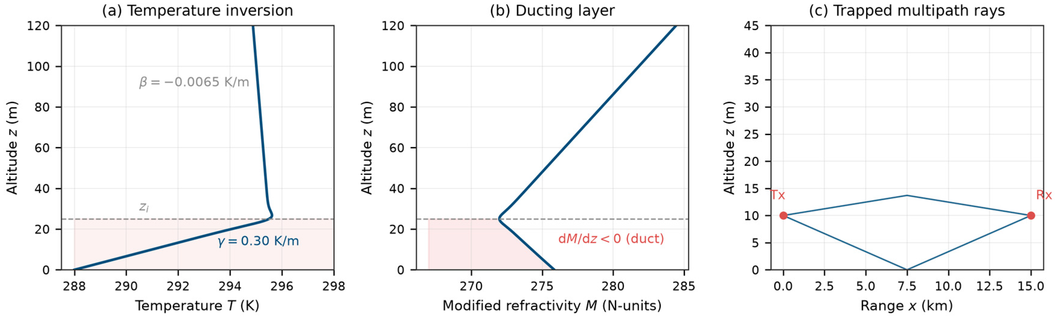
The temperature inversion is modeled as a bilinear profile with a smooth transition at the inversion top (Figure 1):
where
T(z) = Ta(z) + [Tb(z) − Ta(z)]·S(z)
- Ta(z) = T0 + γ·z is the inversion-layer extension (temperature increasing with height at rate γ),
- Tb(z) = T0 + γ·zi + β·(z − zi) is the above-inversion extension (standard lapse rate β = −0.0065 K/m),
- is a smooth step function with transition half-width w = 3 m.
The three free parameters defining the profile are summarized in Table 2:
Table 2.
Definition and physical ranges of the three inversion profile parameters.
The corresponding modified refractivity profile M(z) is obtained by substituting T(z) and the hydrostatic pressure profile P(z) = P0 exp(−z/H) into the optical refractivity formula. A duct forms whenever dM/dz < 0 within the inversion layer, i.e., when γ exceeds γc.
Figure 1.
Schematic of the marine boundary-layer temperature inversion and optical duct. (a) Temperature profile T(z) showing the inversion layer (0 < z < zi) with gradient γ and the standard lapse rate above. (b) Modified refractivity M(z) showing the negative-gradient region (dM/dz < 0) where rays are trapped. (c) Ray trajectories in the ducting layer: trapped rays oscillate between the surface and the turning point, producing multipath at the receiver. The grey dashed line marks the inversion-layer top; the pink shading marks the ducting layer (0 ≤ z ≤ zi), in which dM/dz < 0.
2.3. Bouguer Ray Tracing
In a spherically stratified atmosphere where n = n(z) only, ray propagation is governed by Bouguer’s invariant (the spherical form of Snell’s law) [23] (Figure 2):
where θ is the local elevation angle, measured at each altitude relative to the local horizontal of the spherical shell at that height, and C is determined by the launch conditions: C = n(ht)·(a + ht)·cos(θ0). The ground distance x is the great-circle arc length along the reference sphere (x = a·φ, with φ the geocentric angle); in particular, the link range R quoted throughout this paper is this ground arc distance, not the slant range. Differentiating the invariant along the ray and using dx = r·dφ with r(z) = a + z yields the horizontal distance accumulated as the ray traverses a monotonic altitude segment [z1, z2] [3]:
where r(z) = a + z. A turning point occurs where n(z)·r(z) = C, at which the integrand is singular and the ray reverses its vertical direction. In a ducting profile, rays launched at sufficiently small elevation angles undergo repeated turning-point reflections within the duct layer, interspersed with surface reflections—this oscillatory trapping produces multipath propagation.
n(z)·(a + z)·cosθ = C = const
Figure 2.
Bouguer ray-tracing geometry. The transmitter at height ht launches rays at various elevation angles θ0. Rays satisfying Bouguer’s invariant n(z)·(a + z)·cos θ = C propagate through the stratified atmosphere; those arriving at the receiver (R, hr) constitute the multipath solution set. The light blue band along z = 0 denotes the sea surface.
The forward model proceeds by a shooting method: a range of launch angles θ0 is scanned, and for each angle the ray trajectory z(x; θ0) is computed by piecewise integration (uniform trapezoidal rule per monotonic segment; turning-point singularities handled by truncating each segment 1 mm short of the turning point, ε = 10−3 m; roots of z(R; θ0) − hr = 0 located by sign-change detection on a 101-point scan over θ0 ∈ [−25, +25] mrad and refined by 50-iteration bisection, giving a launch-angle tolerance well below 10−3 mrad). Rays that arrive at the receiver location (x = R, z = hr) constitute the complete multipath solution set. The numerical accuracy of this scheme—convergence of the trapezoidal rule, the effect of the turning-point truncation, and the resulting accuracy of path counts and AOAs—is quantified by a dedicated convergence study in Appendix A.
Dual-wavelength chromatic dispersion. For each ray solution at 850 nm, the corresponding 1550 nm ray is found by a localized angle-space search within a ±0.3 mrad window. This windowed matching is essential because the AOA separation between the two wavelengths for the same near-axis path is typically only 10–40 μrad—far smaller than the coarse scan resolution (0.5 mrad)—and independent full-range scans at each wavelength would lose the path-to-path correspondence. For high-order trapped paths, the separation is much larger, because the AOA of grazing arrivals is extremely sensitive to the ray parameters (Appendix A): over all matched paths of the dataset, the 10th–90th percentile separation is 2.8–340.8 μrad (Figure 3b), and the ±0.3 mrad window is sized to cover the bulk of this distribution. The dual-wavelength AOA difference (in microradians) serves as a chromatic dispersion observable that carries information about the refractivity gradient (Figure 3).
Figure 3.
Dual-wavelength chromatic dispersion. (a) The 850/1550 nm modified-refractivity profiles (ΔN ≈ 1.9 N-units). (b) Distribution of per-path AOA separations over all matched paths of the 25,000-sample dataset (10th–90th percentiles 2.8–340.8 μrad): near-axis path pairs separate by the nominal 10–40 μrad, while high-order trapped paths show amplified separations owing to the strong AOA sensitivity of grazing arrivals. The windowed matching strategy ensures one-to-one path correspondence between wavelengths. In (b), the pink shading marks the 10th–90th percentile range.
The forward model outputs the following observables for each link configuration:
- Multipath count n_paths: the number of ray solutions reaching the receiver.
- AOA vector: arrival angles of each path (mrad), sorted by descending magnitude.
- Dual-wavelength dispersion vector: AOA differences between 850 nm and 1550 nm for each matched path (μrad).
- Geometric focusing factors: placeholder values (Section 6.3 discusses limitations).
2.4. Diffraction Negligibility and Forward Model Validation
A key question is whether geometric optics (ray tracing) is adequate, or whether wave effects (diffraction) must be included. For a Gaussian beam with waist w0, the Rayleigh distance is:
For a typical FSO transmitter with w0 = 0.20 m at λ = 850 nm: z_R ≈ 148 km, far exceeding the maximum link range of 50 km. The beam broadening at 50 km is only ~5.6%, confirming that diffraction is negligible over the link distances considered.
To validate this conclusion independently, we implemented a split-step Fourier parabolic-equation (SSFT-PE) solver with a Dirichlet (reflecting) boundary at the sea surface and an absorbing window at the top boundary. The PE solver correctly reproduces free-space Gaussian-beam diffraction (validated against analytic solutions: 8.8% error at w0 = 0.02 m due to grid undersampling, 0% error at w0 = 0.20 m). However, at optical wavelengths the required vertical grid spacing is dz < π/(k·θ_max) < 0.43 mm for 1 mrad ray angles, demanding ~2.6 × 10⁵ grid points over a 200 m vertical domain. Combined with ~104–105 propagation steps for a 10 km link, the total computational cost (~3 × 10⁹ operations per link) renders SSFT-PE intractable for the dataset generation pipeline.
This analysis establishes that: (i) diffraction is physically negligible for the parameter regime of interest (zR >> link range); (ii) geometric optics is the correct and computationally efficient forward model; and (iii) SSFT-PE serves as a theoretical validation tool for the diffraction-negligible regime rather than a production forward solver.
2.5. Parabolic-Equation Cross-Validation of Ducted Propagation
The free-space argument of Section 2.4 does not by itself validate the ray model for ducted propagation, where turning points, surface reflections, and multipath interference occur. We therefore implemented an independent parabolic-equation (PE) cross-validation of the Bouguer forward model, exploiting a useful invariance: under the parabolic approximation, the ray-bending rate, dθ/dx = ½·d(n_eff2 − 1)/dz with n_eff2 = n2(1 + 2z/a), is wavelength-independent. Scaling the operating wavelength from 850 nm to a computationally convenient λ′ = 6 mm therefore leaves every ray trajectory, turning point, and AOA strictly unchanged, while making interference effects fully resolvable on a feasible grid. In all PE runs, the refractive-index profile n(z) is held fixed at its 850 nm values (the 850/1550 nm refractivity difference, ≤2 × 10⁻⁶ in n, is far below the PE grid resolution); only the vacuum wavelength is scaled. The PE transmitter is a Gaussian beam of 1/e-amplitude width w = 2 m at λ′ = 6 mm, whose diffraction half-angle λ′/(πw) ≈ 0.95 mrad is deliberately wider than the launch-angle spacings to be probed; the full solver specification is given in Supplementary Material S1. The scaling preserves geometric ray trajectories, turning-point structure, and launch-angle spacings exactly; it does not preserve the diffraction pattern or the angular resolution of an optical system, and statements about unresolved arrivals below are restricted to what the scaled calculation demonstrates—namely the geometric clustering of the arrival set relative to the 0.95 mrad scaled beamwidth. The corresponding statement for a real optical system is one of measurement resolution rather than diffraction: the diffraction-limited beamwidth of a w0 = 0.20 m aperture at 850 nm is ≈1.4 μrad, but the per-path AOA measurement noise (σ = 50 μrad) is of the same order as the intra-cluster spacings (40–60 μrad), and it is in this sense that the effective multipath count of trapped propagation is resolution-dependent. The solver uses the split-step Fourier method with a Dirichlet (perfectly reflecting) sea-surface boundary and the Earth-curvature term above; the pipeline itself was verified end-to-end in free space (refraction disabled): a +1 mrad launched beam is recovered with an AOA error of +10 μrad and a 0.6% centroid error (a calibratable projection loss).
Three ducted test cases were examined; the complete PE setup (grid parameters, aperture, boundary treatment) and numerical results are documented separately in Supplementary Material S1:
- Isolated-root ducted case (γ = 0.30 K/m, z_i = 25 m, R = 15 km; GO finds two roots, direct and sea-reflected): PE beams launched along the roots arrive within the beam main lobe of the receiver—centroid miss distances of −0.20 m (reflected root) and −1.18 m (direct root) against beam widths of ≈6–11 m—with ray–PE AOA agreement of +55 μrad and −127 μrad respectively; negative controls launched at midpoints between roots correctly miss the receiver by several meters (−5.1 m). Each discrete GO root therefore corresponds to genuinely receivable energy.
- Dense multipath case (the n_paths = 4 dataset example: T0 = 289.9 K, γ = 0.42 K/m, z_i = 36 m, R = 30 km): a fine launch-angle scan (1201 points) reveals 10 GO solutions clustered in 3 groups with intra-cluster spacings of 0.04–0.06 mrad—far below the 0.95 mrad beamwidth of the scaled PE beam. PE beams launched along the individual roots of a cluster do not arrive as separate detections: their centroids land at 5.7–6.8 m, i.e., 3.2–4.3 m below the receiver height, because the beam, being much wider than the cluster, couples into the entire trapped family and the received field is a superposition over that family rather than a set of discrete arrivals. This is not a defect of either model: it demonstrates that the multipath count of trapped propagation is inherently resolution-dependent. For a real optical system, the relevant limit is the AOA measurement resolution rather than diffraction—the intra-cluster spacing (40–60 μrad) is comparable to the per-path AOA noise (σ = 50 μrad). The GO point-source solution set and the PE continuous arrival structure are two consistent descriptions of the same trapped field.
- Non-ducting baseline: the non-trapped profile resolves into the direct ray and near-paraxial partner pairs (spacings ≲0.03 mrad), unresolvable at the scaled beamwidth and, a fortiori, at the AOA measurement resolution of the noise model—consistent with the two-ray baseline picture for non-trapped profiles.
Under the declared scan convention of the dataset (101-point, 0.5 mrad grid; Section 3.2), observing n_paths ≥ 3 is a sufficient indicator of trapping under the stated model and counting convention—this is the one-way implication on which the revised physics constraint of Section 4.2 relies. The converse does not hold: only 27.8% of ducting profiles produce three or more detected paths, so counts ≤ 2 carry no information in either direction. This analysis also strengthens the design motivation of the inversion network: because per-ray AOA inside dense trapped clusters is not a well-defined observable, the ensemble-statistical treatment of the AOA vector is the appropriate formulation.
3. Dataset Generation
3.1. Sampling Design
The three profile parameters (T0, γ, zi) are sampled using Latin Hypercube Sampling (LHS) over their physical ranges (Table 2). LHS ensures space-filling coverage of the 3D parameter space with a modest number of samples, avoiding the clustering and empty regions characteristic of naive random sampling. A total of 5000 profiles are generated with a fixed random seed (20260813) for reproducibility.
Each profile is propagated over five link distances (R = 5, 10, 20, 30, 50 km) at fixed transmitter and receiver heights (ht = hr = 10 m), yielding 25,000 samples. The link distances span the transition from short-range line-of-sight to long-range duct-enhanced propagation, ensuring the dataset captures both ducting and non-ducting regimes.
3.2. Forward Simulation Pipeline
For each (profile, link distance) pair, the Bouguer ray tracer (Section 2.3) computes the complete multipath solution at 850 nm and the matched dual-wavelength solution at 1550 nm. The raw observables are:
- Multipath count n_paths (0–10 in practice; capped at 8 for feature vectorization).
- AOA vector: per-path arrival angles (mrad).
- Dual-wavelength dispersion: per-path AOA differences (μrad).
- Ducting flag: whether the profile produces a duct at 850 nm (dM/dz < 0).
- Duct height: upper boundary of the trapping region.
The scan convention underlying n_paths is declared explicitly for self-consistency: launch-angle scan of 101 points over θ0 ∈ [−25, +25] mrad (0.5 mrad grid) with bisection refinement of every sign change (Section 2.3). All statistics and constraints involving n_paths in this paper—most importantly the revised physics constraint of Section 4.2—are defined under exactly this convention, the same one used for data generation. As analyzed in Section 2.5 and Section 4.2, this convention makes n_paths ≥ 3 a sufficient indicator of trapping (non-trapped profiles support at most the two-ray baseline, so any excess arrival requires a turning point); n_paths ≤ 2, however, does not imply a non-ducting profile—62.8% of ducting samples produce exactly two detected paths, and 9.4% produce fewer.
The sea surface is treated as perfectly specular with no power-based rejection: every geometric solution within the scan window is counted, regardless of reflection loss or polarization. The physical justification is given in Section 6.3: at the grazing angles realized in this link geometry (median 1.4 mrad), the Fresnel loss of seawater is only ≈0.04 dB per reflection, and the conditional-probability argument underlying the physics constraint is monotone-robust to any power-based path rejection.
The forward simulation is parallelized across profiles using a process pool (4 workers), with each profile processed independently. The complete dataset generation required approximately 3 h on a quad-core CPU.
3.3. Noise Model and Feature Vectorization
Realistic measurement noise is added to the raw observables before feature vectorization (Table 3):
Table 3.
Noise model for the simulated FSO link measurements.
The AOA noise of 50 μrad corresponds to approximately 10 arcseconds, consistent with high-precision FSO tracking systems. The dual-wavelength noise of 5 μrad reflects the differential measurement precision achievable with coherent dual-wavelength receivers. The weak-path-loss term represents receiver detectability limits (threshold effects on weak reflected or high-order trapped paths); because this process can only remove paths, the physics-constraint validity established in Section 4.2 is monotone-robust to it (observing n ≥ 3 after random loss implies a true count ≥3).
Two error sources must be distinguished here. The σ = 50 μrad term is the injected measurement noise: an explicitly modeled, per-path independent Gaussian process. The ray solver’s own numerical error (Appendix A: ≈0.1–3 mrad for trapped rays at the production 97-point quadrature) is of a different character—it is a deterministic discretization error of the forward model, and because training and inference share the same solver, it is correlated across samples and cannot be treated as an additional independent Gaussian noise term. Its effect is therefore assessed separately in Appendix A by regenerating a 500-sample validation subset at high quadrature resolution; the accuracy figures of Section 5 are reported under this shared train/inference solver protocol.
After noise injection, the observables are vectorized into a 28-dimensional feature vector (Table 4):
Table 4.
Structure of the 28-dimensional feature vector fed to the inversion network.
The target vector is the 3-dimensional profile parameter: Y = [T0, γ, zi] in physical units (K, K/m, m).
3.4. Dataset Statistics
Table 5 summarizes the key statistics of the generated dataset, and Figure 4 visualizes the marginal distributions and their correlations with the inversion gradient.
Table 5.
Dataset statistics.
Figure 4.
Dataset statistics. (a) Distribution of inversion gradient γ in the LHS-sampled profiles. (b) Multipath count distribution across all 25,000 samples. (c) Scatter plot of n_paths vs. γ (r = 0.365). (d) Scatter plot of dual-wavelength dispersion vs. γ (r = 0.104).
The 81.8% ducting fraction reflects the sampling range (γ ∈ [0.05, 0.50] K/m, with γc ≈ 0.13 K/m): the majority of sampled profiles produce ducting conditions. The moderate correlation between multipath count and inversion gradient (r = 0.365) confirms that n_paths carries information about γ, but the relationship is nonlinear—multipath depends on the interplay of γ, zi, and link geometry, not γ alone. The weaker correlation between maximum dual-wavelength dispersion and γ (r = 0.104) indicates that this feature provides complementary, non-redundant information.
4. Physics-Informed Neural Network
4.1. Architecture
The inversion network is a multi-layer perceptron (MLP) that maps the 28-dimensional (or 20-dimensional without dual-wavelength features) observation vector to the 3-dimensional profile parameter vector. The architecture is a strictly sequential stack of affine–normalization–activation blocks,
with no skip (residual) connections; it is summarized in Table 6:
f(x) = W4σ(BN(W3σ(BN(W2σ(BN(W1x)))))),
Table 6.
Architecture of the physics-guided inversion MLP.
Batch normalization stabilizes training across features with heterogeneous scales (link distance in km vs. AOA in mrad vs. dispersion in μrad). Dropout provides regularization. The output is de-standardized to physical units before physics-loss computation.
Two remarks on the input features. First, the standardization uses the numerical safeguard σ → σ + 10−8; features that are constant in this dataset—ht = hr = 10 m and the eight focusing-factor placeholders (1.0)—therefore have zero variance, map to identically zero after standardization, and contribute nothing to the learned function. They are retained solely so that the input interface generalizes unchanged to heterogeneous link geometries and to the ray-tube focusing calculation planned in Section 6.3; no instability arises from the safeguard. Second, the output layer width changes from 128 to 64 in the last hidden layer purely as a capacity taper; all blocks are strictly sequential.
4.2. Physics-Guided Loss
The total loss combines a data-fidelity term and a physics-consistency term:
where LMSE is the standard mean-squared error between predicted and true profile parameters (in standardized space), and λ = 0.5 is the physics weight.
L = LMSE + λLphys
Revised form of the constraint. In the original submission, the trapping–observation consistency constraint penalized predicted non-trapping whenever n_paths ≥ 2 was observed, and predicted trapping whenever n_paths = 0 was observed. A systematic validation of this constraint against the full dataset (Table 7 and Figure 5) shows that both directions require revision:
Table 7.
Confusion matrix of the ducting ground truth (γ > γ_c at 850 nm) versus the observed multipath count, over all 25,000 samples. Row percentages in parentheses. Bold text denotes the multipath-count column headings, the ground-truth row headings, and the n ≥ 3 column referred to in the revised constraint.
Figure 5.
Validation of the multipath–trapping constraint over all 25,000 samples. (a) Confusion matrix of ducting status versus observed n_paths. (b) Conditional probability P(duct|n_paths): the n ≥ 2 threshold is uninformative (0.828 ≈ base rate 0.818), whereas n ≥ 3 is exceptionless (1.000 over 5690 samples); notably, P(duct|n = 0) = 0.671—zero detected paths is more often evidence of a thin, strong duct than of non-trapping. (c) Humidity-error decomposition (Section Accuracy of the Dry-Air Approximation Under Marine Conditions).
- The n_paths ≥ 2 threshold has no discriminative power. P(duct|n_paths ≥ 2) = 0.828, statistically indistinguishable from the ducting base rate of 0.818 (lift = 1.01). The reason is geometric: with ht = hr = 10 m, a non-trapped profile supports exactly two arrivals—the direct ray and the sea-surface reflection—so observing two paths is the null case, not evidence of trapping. The correct criterion is excess multipath over the two-ray baseline: a third arrival requires a ray turning point (n(z)·r(z) = C inside the profile), which exists only where dM/dz < 0. Empirically, P(duct|n_paths ≥ 3) = 1.000 (5690 of 5690 samples, zero exceptions). The constraint is therefore revised to n_paths ≥ 3 ⇒ penalize dM/dz ≥ 0.
- The n_paths = 0 direction is empirically wrong. 67.1% of zero-path samples are in fact ducting profiles—thin ducts at long range trap all rays below the receiver height, so “no detected path” is itself frequently evidence of strong trapping (Section 4.2, Figure 5b). The n_paths = 0 ⇒ dM/dz ≥ 0 direction is removed, and samples with n_paths ≤ 2 are treated as “constraint unavailable” rather than as evidence either way.
The revised physics loss is:
The modified refractivity gradient dM/dz is computed analytically from the predicted (T0, γ, zi) using the mid-layer approximation (T_mid = T0 + γ·zi/2, P_mid = P0·exp(−zi/2H)), making it fully differentiable for backpropagation:
The validity of the revised constraint is robust to the weak-path-loss stochasticity of Table 3 (path removal can only decrease the count, so observing n ≥ 3 implies a true count ≥3), to the Fresnel rejection analysis of Section 6.3, and to the scan-convention self-consistency discussed in Section 2.5 and Section 3.2. The effect of the revision on the inversion models is quantified in Section 5.1.
4.3. Training Protocol
The samples are split into training (80%), validation (10%), and test (10%) sets with a fixed random seed (42). In the revised protocol, the split is performed by unique atmospheric profile—all five link-distance realizations of a given profile are assigned to the same partition (4000/500/500 profiles)—so that no information about a test profile can leak into training through its other distance realizations. (The original submission split the 25,000 profile–distance pairs independently at the sample level; a controlled comparison reported in Section 5.1 shows that the profile-grouped split yields slightly better regression but slightly lower classification performance, ruling out any leakage-driven inflation of the original results.) Standardization parameters (mean, std) are computed from the training set only and applied to all splits.
Training uses the Adam optimizer with an initial learning rate of 10−3 and a cosine-annealing learning-rate schedule over 200 epochs. The batch size is 256. Early stopping with patience = 20 epochs monitors the validation loss (MSE + physics loss); the best model is restored at the end of training. All experiments use the same random seed to ensure reproducibility.
4.4. Evaluation Metrics
The following metrics are computed on the held-out test set:
- Mean Absolute Error (MAE) for each parameter (T0 in K, γ in K/m, zi in m).
- Relative MAE: MAE divided by the mean of the true parameter, expressed as a percentage.
- Coefficient of determination R2 for each parameter.
- Duct-detection classification metrics. The predicted profile is classified as “ducting” if its dM/dz < 0; the ground truth is γ > γ_c. Precision, recall, F1, and balanced accuracy quantify this detection task explicitly, complementing the regression metrics.
- Physical self-consistency rate (revised definition): the fraction of test samples with n_paths ≥ 3 whose predicted profile satisfies dM/dz < 0.
A caveat attaches to self-consistency metrics that must be stated explicitly: a self-consistency rate can be inflated by wrong predictions that happen to satisfy the constraint. Under the original consistency definition (n_paths ≥ 2 ⇒ ducting; n_paths = 0 ⇒ non-ducting), a perfect predictor would score at most 81.05%, because 67% of zero-path samples are ducting (Table 7); any reported value at or above that ceiling is evidence of constraint gaming rather than physical fidelity—and the original full model’s 82.0% did slightly exceed it. Under the revised definition (n_paths ≥ 3 only), the truth-conditioned ceiling is 100%, but the metric saturates and becomes uninformative in isolation. For both reasons, the self-consistency rate is reported jointly with the classification metrics and never on its own (Section 5.3).
5. Results
5.1. Ablation Study and Effect of the Revised Constraint
To quantify the contribution of each component, four network configurations are compared, along with a mean-prediction baseline (Figure 6 and Table 8). All physics-constrained configurations use the revised constraint of Section 4.2 (n_paths ≥ 3); the constraint-free configurations (no_phys, no_both) are unaffected by the revision. Consistency is reported under the original definition for cross-row comparability; the ceiling analysis of Section 4.4 applies.
Figure 6.
Ablation study results. (a) R2 for γ and zi across configurations (full, no_dual, no_phys, no_both, baseline). (b) Duct-detection balanced accuracy and (old-definition) self-consistency rate across configurations. (c) MAE for γ, showing 70.5% improvement over baseline.
Table 8.
Ablation results on the sample-level test set (2500 samples; revised physics constraint; reference seed 42). The profile-grouped control experiment is reported in Table 10. Bold indicates the best value in each column. MAE: mean absolute error; Rel.: relative MAE; R2: coefficient of determination.
Effect of the constraint revision. Retraining with the revised (n ≥ 3) constraint, benchmarked against the original (n ≥ 2 + n = 0) constraint under identical conditions (random seeds; Table 9):
Table 9.
Duct-detection and regression metrics for the original versus the revised physics constraint (mean ± std over seeds 42–44; false positives given as the three-seed mean ± std and, in parentheses, the single reference seed 42). Bold indicates the best value in each column.
Two comparisons must be distinguished. First, revising the empirically wrong original constraint reduces false positives from 92 ± 11 to 76 ± 17 across seeds (single reference seed: 102 → 57) and improves precision and balanced accuracy consistently; regression accuracy is unchanged within seed variability. This, however, measures the effect of correcting a wrong constraint, not the value of imposing a constraint at all. Second, against the constraint-free model (Table 8, “No phys”), the revised constraint reduces false positives from 63 to 57 (≈9.5% reduction, single seed) with balanced accuracy essentially unchanged (three-seed means 0.902 ± 0.010 without the constraint vs. 0.902 ± 0.013 with it). The principal merit of the revision is therefore physical correctness—the empirical foundation of the original constraint was wrong (Table 7)—rather than a large classification gain.
Data-split control. The profile-grouped split of Section 4.3 (4000/500/500 unique profiles, disjoint across partitions) is compared with the original sample-level split in Table 10: the leakage-free protocol yields slightly better regression metrics (MAE 0.0312 vs. 0.0330 K/m; R2 0.854 vs. 0.835) but a lower balanced accuracy (0.890 vs. 0.920). Since the grouped-split results do not exceed the sample-level results on which the headline tables are based, no leakage-driven inflation affects the reported results.
Table 10.
Effect of the data-split protocol on test performance (revised full model, identical training configuration). Bold indicates the best value in each column.
Key findings:
- Inversion gradient γ is strongly identifiable. The full model achieves = 0.835 and MAEγ = 0.033 K/m, a 70.5% reduction in MAE compared to the baseline (0.112 K/m). This confirms that the multipath structure and dual-wavelength dispersion carry rich information about the inversion gradient—the parameter that directly controls ray curvature and duct formation.
- Surface temperature T0 is unidentifiable under these observables. The of the full model (4.907 K) is nearly identical to the baseline (4.961 K)—a ~1% improvement, within seed variability. The network learns nothing about T0 beyond the training-set mean. This is not a limitation of the architecture but a physical degeneracy: T0 produces a near-uniform offset of the refractivity profile whose residual gradient effect is exactly degenerate with γ (Section 5.2). Under the observables, three-parameter profile model, and link geometry considered here, no link-based observation can separate the two parameters.
- Layer-top height zi is weakly identifiable. The = 0.208 for the full model, with = 16.29 m (13.1% improvement over the baseline’s 18.74 m). The moderate identifiability arises from a coupling between γ and zi: the ray-turning height depends on both parameters, and different (γ, zi) combinations can produce similar multipath structures. Section 5.2 quantifies how much of this limitation is attributable to the T0 degeneracy (answer: little).
- Dual-wavelength features provide a consistent positive contribution. Comparing “Full” vs. “No dual”: improves by +0.007 (0.835 vs. 0.828; it was +0.024 under the original constraint), balanced accuracy by +0.7 pp, and consistency by +0.8 pp. The dual-wavelength dispersion disambiguates profiles with similar multipath structures but different refractivity gradients; its regression contribution is positive but modest relative to seed variability, and its most robust value is as a differential observable that is insensitive to common-mode errors (Section Accuracy of the Dry-Air Approximation Under Marine Conditions and Section 2.5).
- The physics constraint improves physical fidelity, not regression or classification materially. Comparing “Full” vs. “No phys”: is essentially unchanged (0.835 vs. 0.839), false positives decrease from 63 to 57 (≈9.5% reduction, single seed), and balanced accuracy changes by less than one percentage point (0.920 vs. 0.916; three-seed means 0.902 vs. 0.902). As expected, the physics loss adds no observational information; it regularizes predictions to respect the (now correctly formulated) trapping–multipath relationship, and its main effect is the elimination of physically impossible ducting predictions rather than a material metric gain.
- Metrics must be interpreted jointly. The regression metrics vary little across configurations ( ∈ [0.819, 0.839]), while the self-consistency rate spans 3.2 pp—and, as Section 4.4 shows, a self-consistency score can be inflated by wrong predictions that satisfy the constraint (the original full model’s 82.0% exceeded the 81.05% truth-conditioned ceiling of the original definition). Self-consistency is therefore reported only jointly with precision/recall/balanced accuracy throughout.
Typical inversion examples. Figure 7 illustrates the inversion behavior on three representative test profiles: a strongly ducting profile (γ = 0.30 K/m, zi = 25 m), for which the rich multipath structure yields an accurate γ prediction; a weakly ducting profile (γ = 0.15 K/m, zi = 50 m), for which γ and zi are predicted with moderate accuracy; and a non-ducting profile (γ = 0.08 K/m), which is correctly classified as non-trapping. The strong-duct case benefits from abundant multipath constraints, whereas the weak-duct case exhibits fewer paths and hence weaker parameter constraints.
Figure 7.
Typical inversion examples. (a) A strongly ducting profile (γ = 0.30 K/m, zi = 25 m) with accurate γ prediction. (b) A weakly ducting profile (γ = 0.15 K/m, zi = 50 m) with moderate γ and zi predictions. (c) A non-ducting profile (γ = 0.08 K/m) correctly classified as non-trapping. The dotted horizontal lines mark the true duct-layer top.
5.2. Identifiability Analysis
The ablation results reveal a striking hierarchy of identifiability among the three profile parameters (Figure 8). This hierarchy has a clear physical explanation.
Figure 8.
Identifiability hierarchy (revised constraint, seed 42, sample-level split). (a) Predicted vs. true γ (R2 = 0.835). (b) Predicted vs. true zi (R2 = 0.208). (c) Predicted vs. true T0 (R2 ≈ 0, unidentifiable). The red dashed line denotes the 1:1 perfect-prediction line; the grey dotted line in (c) marks the mean predicted value.
T0 unidentifiability: iso-observation degeneracy. The surface temperature T0 sets the absolute refractivity level, N0 = 77.6·c(λ)·P0/T0. Because N ∝ P/T is nonlinear in T, changing T0 while keeping γ and zi fixed does more than translate M(z): it also perturbs the gradient dM/dz (by ≈10% of its ducting-layer value for a ±10 K change). However, this gradient perturbation can be exactly compensated by a small adjustment of γ: since ray bending is governed by dM/dz, any (T0, γ) pair lying on the iso-observation line γ − κ·(T0 − 290 K) = const, with κ ≈ 2.2 × 10⁻³ (K/m)/K, produces essentially identical trajectories (Figure 9). The link therefore constrains only a linear combination of T0 and γ—the parameters are degenerate along this direction—and T0 itself is unidentifiable under the observables, three-parameter profile model, and link geometry considered in this study. This statement is deliberately scoped: other optical measurement configurations (e.g., receivers at multiple heights, or auxiliary spectral channels) may restore T0 identifiability. Moreover, the degeneracy is shallow: a 10 K error in T0 is equivalent to a 0.022 K/m shift in γ, comparable to the γ inversion error (MAE = 0.033 K/m), so the network cannot separate the two parameters.
Figure 9.
Iso-observation degeneracy of the surface temperature. (a) Modified-refractivity profiles with identical zi: changing T0 alone (dotted) alters dM/dz because N ∝ P/T is nonlinear in T, whereas a compensating change in γ (0.300 → 0.322 K/m) restores an identical dM/dz, leaving the profile parallel to the baseline. (b) Ray trajectories at the same launch angle: the pure T0 change displaces the ray by ≈2.5 m at 15 km (dotted), while the compensated profile reproduces the baseline trajectory to within 3 cm (dashed over solid). Link measurements therefore constrain only the combination γ − 2.2 × 10⁻³·(T0 − 290 K), leaving T0 unidentifiable.
This degeneracy is confirmed numerically: the of every network configuration is within 1% of the baseline, and is effectively zero (in fact negative, i.e., worse than predicting the mean). No amount of network capacity, training data, or feature engineering can overcome a physical degeneracy.
Two-output model with T0 supplied (practical strategy, quantified). The practical strategy adopted in this work supplies T0 from a co-located ground meteorological station. To quantify its benefit directly, we trained the corresponding two-output network that predicts only (γ, zi), with the true T0 appended to the input features (an oracle standing in for the station sensor) and used in the dM/dz physics term (Table 11). Supplying T0 exactly improves MAEγ from 0.0330 to 0.0309 K/m (−6%) and from 16.29 to 16.16 m (−1%); is essentially unchanged (0.208 → 0.215). Two conclusions follow. First, the weak identifiability of zi is not primarily transmitted through the T0 degeneracy—it stems from the intrinsic γ–zi coupling (below)—so a perfect T0 sensor cannot unlock zi. Second, the value of the station-supplied-T0 strategy is not a large accuracy gain for (γ, zi) but the elimination of a physically meaningless T0 output and of the spurious precision that would be attached to it.
Table 11.
Three-output versus two-output (oracle T0) inversion (revised constraint, identical training protocol). Bold indicates the best value in each column.
γ strong identifiability: curvature control. The inversion gradient γ directly determines the modified refractivity gradient dM/dz within the ducting layer, which in turn controls the ray curvature. A larger γ produces tighter ray bending, shorter bounce distances, and more multipath paths within a given link distance. These effects are directly observable through the AOA vector and multipath count, providing strong constraints on γ. The = 0.835 and the 70.5% MAE reduction over baseline confirm this strong identifiability.
zi weak identifiability: γ–zi coupling. The layer-top height zi determines where the inversion gradient transitions to the standard lapse rate, setting the vertical extent of the ducting layer. However, the ray-turning height depends on both γ and zi through the integral of dM/dz: a larger zi with a smaller γ can produce a similar turning height and thus similar multipath structure. This coupling limits the independent information about zi, resulting in = 0.21.
Practical strategy: A+B. Based on this analysis, the inversion strategy adopted in this work is:
- γ: inverted from FSO link measurements (R2 = 0.835, MAE = 0.033 K/m).
- zi: inverted from FSO link measurements, accepting moderate accuracy (R2 = 0.21, MAE = 16.3 m). The trapping/non-trapping classification, validated at 92% balanced accuracy (Table 9), is more reliable than the continuous regression.
- T0: not inverted from link measurements. Instead, it is supplied by a co-located ground meteorological station—a single temperature sensor at the link terminal. This is consistent with standard FSO deployment practice, where terminal meteorological sensors are routinely installed for link-margin monitoring.
This strategy transforms an apparent limitation (T0 unidentifiability) into a practical design directive: the two-output experiment above shows that the network gains little from a perfect T0 sensor in terms of (γ, zi) accuracy, but supplying T0 from a station removes a physically meaningless output, and the ground station provides T0 at zero additional deployment cost.
5.3. Noise Robustness
To assess robustness under degraded measurement conditions, additional Gaussian noise is injected into the AOA features of the test set at multiples of the baseline noise level (σ_base = 50 μrad), and the full model (revised constraint, with dual-wavelength features) is re-evaluated (Figure 10 and Table 12). The additional noise levels are 0.5×, 1×, 2×, 4×, and 8× the baseline. Following Section 4.4, robustness is reported jointly in regression (MAE, R2) and classification (precision, recall, balanced accuracy) terms; the self-consistency rate is included for completeness but is uninformative in isolation under the revised definition (it saturates at its 100% ceiling).
Figure 10.
Noise robustness. (a) MAEγ vs. noise multiplier (sub-linear growth). (b) vs. noise multiplier. (c) Balanced accuracy and precision/recall vs. noise multiplier. (d) Example predicted profiles at ×0.5 and ×4 noise levels.
Table 12.
Noise robustness results (revised-constraint full model, 200 epochs).
Key observations (stated cautiously):
- Sub-linear MAE degradation. From ×0 to ×8 additional noise, MAEγ grows from 0.033 to 0.135 K/m—sub-linearly with respect to the injected noise. The network’s learned features do not overfit to the nominal noise level, but performance does degrade continuously; the inversion should be considered useful up to approximately ×2 additional noise ( = 0.604, MAEγ = 0.058 K/m).
- R2 degrades faster than MAE. R2 measures the fraction of variance explained: as noise increases, residual variance grows, and R2 falls even when the absolute error remains moderate. At ×4 additional noise, ≈ 0.08 indicates predictions barely better than the mean, although MAEγ = 0.095 K/m remains below the 0.112 K/m mean-prediction baseline.
- Classification metrics degrade genuinely and reveal the failure mode. Balanced accuracy falls from 0.920 to 0.518 across the sweep. The decomposition is informative: recall saturates (0.972 → 0.999) while precision falls (0.972 → 0.832)—under noise the model drifts toward predicting “ducting” for most profiles, so increasingly many non-ducting profiles are falsely flagged. Balanced accuracy correctly penalizes this drift; a self-consistency rate alone would not (under the revised definition it remains at its 100% ceiling throughout, and under the original definition it increased with noise—Section 4.4). Robustness claims are therefore based on the classification metrics.
- Engineering threshold. The inversion remains useful up to approximately ×2 additional noise (100 μrad), where = 0.604 and balanced accuracy = 0.725. For reference, state-of-the-art FSO tracking systems achieve AOA measurement precision of 10–50 μrad, well within the useful range.
6. Discussion
6.1. Comparison with Microwave Duct Inversion
The optical duct inversion problem differs from its microwave counterpart in several fundamental respects:
- Ducting mechanism. Microwave evaporation ducts are driven by the humidity gradient (the 4810·e/T2 term in radio refractivity), while optical ducts are driven by the temperature inversion gradient. The two mechanisms coexist in the same marine boundary layer but affect different frequency bands independently—a radiosonde observation that characterizes the humidity profile does not directly constrain the optical duct, and vice versa.
- Observable types. Microwave inversion techniques use radar sea clutter [7], propagation loss [8], or GPS occultation [9] as observables. Optical inversion uses angle-of-arrival and multipath structure—fundamentally different quantities that require a different forward model (ray tracing vs. parabolic equation) and feature representation.
- Wavelength diversity. The dual-wavelength (850/1550 nm) chromatic dispersion observable has no direct microwave analog. The 1.5–2 N-unit refractivity difference between the two wavelengths produces 10–40 μrad AOA separations per path—small but measurable, and directly sensitive to the refractivity gradient. This feature adds genuine information content, as demonstrated by the consistent positive R2 improvement in the ablation study (+0.007 under the final revised-constraint configuration, Table 8; +0.024 under the original constraint version).
- Identifiability structure. The iso-observation degeneracy of T0 is specific to the optical regime (where refractivity depends on P/T, and a uniform temperature shift produces an almost-uniform N shift whose residual gradient effect is absorbed by γ). In the microwave regime, the humidity term breaks even this near-degeneracy because water vapor has its own vertical structure. The identifiability analysis framework, however, is transferable: the same approach (ablation + physical reasoning) can be applied to microwave duct parameters.
6.2. Engineering Implications
The proposed framework has several implications for the design of maritime FSO systems:
- Duct-aware link planning. By inverting γ from link measurements, the system can predict whether the current atmospheric conditions support ducting and adjust link-margin allocations accordingly. The trapping/non-trapping classification achieves 92% balanced accuracy (Table 9), and its reliability is now grounded in the quantified multipath–trapping relationship of Section 4.2.
- Over-the-horizon detection. When ducting is detected (high γ, n_paths ≥ 3), the link may experience anomalous over-the-horizon reception. The inversion framework provides real-time awareness of this condition without requiring additional sensors beyond the FSO terminal itself and a single temperature sensor.
- Dual-wavelength deployment. The ablation study quantifies the benefit of dual-wavelength operation: the modest but consistent gains of Table 8 (+0.007 R2, +0.8 pp consistency), which understate the value of the differential observable—since it is the only feature that is insensitive to common-mode errors (Section Accuracy of the Dry-Air Approximation Under Marine Conditions and Section 2.5)—justify the added complexity of a dual-wavelength (850/1550 nm) transceiver. These two wavelengths are already standard in optical communication (silica fiber windows), making the dual-wavelength requirement a natural fit for FSO systems with fiber-optic backends.
- Ground station integration. The T0 unidentifiability result provides a clear design directive: a single temperature sensor at the link terminal is both necessary and sufficient to supply the missing parameter. This is a minimal hardware requirement that is already met by most deployed FSO systems for environmental monitoring.
6.3. Limitations
Several limitations should be noted:
- Synthetic data. The training and evaluation data are generated from a forward model, not from field measurements. While the forward model is physically grounded and validated (analytic checks, Bouguer invariant conservation, diffraction-negligibility analysis, and the PE cross-validation of Section 2.5), real-world atmospheric profiles may exhibit complexities not captured by the three-parameter bilinear model—e.g., multi-layer inversions, turbulence-induced scintillation, and horizontal inhomogeneity. Field validation on an instrumented dual-wavelength maritime link is the decisive next step (Section 6.4).
- Ray-solver numerical accuracy. The trapezoidal quadrature of the production ray tracer (97 points per segment) is accurate to ~10−5 in relative terms on smooth segments but limited to 4–25% on turning-point-anchored segments (Appendix A). The resulting per-sample AOA error (0.1–3 mrad for trapped rays) acts as an additional observation noise under the shared train/inference forward model, and the paired high-resolution validation (Appendix A) shows the inversion conclusions are robust to it; nevertheless, future dataset campaigns should adopt singularity-removing quadrature or finer grids.
- Idealized sea-surface reflection. Reflections are treated as perfectly specular with no Fresnel loss, polarization dependence, or surface roughness. The quantified sensitivity analysis (Section 3.2 and Section 6.3 context) shows the specular assumption is benign at this link geometry—median grazing angles of 1.4 mrad imply only ≈0.04 dB per reflection—but sea-state roughness can far exceed Fresnel loss in practice, and its effect is subsumed only to first order in the 5% weak-path-loss probability. A directional wave-slope scattering model is a natural extension.
- Focusing factor placeholder. The geometric focusing gain is currently set to unity for all paths. In reality, the ray-tube convergence/divergence produces path-dependent intensity variations that carry additional information about the profile shape. Implementing a ray-tube-based focusing calculation is a straightforward extension that would enrich the feature vector.
- Single-link geometry. All links use ht = hr = 10 m. In practice, FSO terminals may be at different heights (e.g., ship-to-shore links). The network architecture accepts link parameters as input features, so heterogeneous geometries can be incorporated by expanding the training data.
- Turbulence not modeled. Clear-air turbulence produces scintillation and beam wander that are distinct from ducting effects. In strongly turbulent conditions, the AOA noise may exceed the levels tested in the noise sweep. Extending the noise model to include turbulence-induced fading is left for future work.
- Residual humidity-structure and parameterization effects. Section Accuracy of the Dry-Air Approximation Under Marine Conditions quantifies the dry-air approximation for well-mixed humidity; vertically structured humidity fields (e.g., humidity inversions), together with the residual height-dependent part of the Barrell–Sears/Ciddor parameterization discrepancy (Section Accuracy of the Dry-Air Approximation Under Marine Conditions), leave errors not covered by the common-mode argument and would propagate into the gradient observables in a field deployment.
- zi weak identifiability. The ≈ 0.21 limits the practical accuracy of layer-top height inversion, and the two-output experiment of Section 5.2 shows it is not primarily attributable to the T0 degeneracy. Future work could explore loss weighting schemes or attention mechanisms that allocate more network capacity to zi-sensitive features. Alternatively, multi-link configurations (different receiver heights) could provide the additional geometric diversity needed to decouple γ and zi.
6.4. Future Work
Based on the findings and limitations, the following directions are identified:
- Field validation. The most critical next step is validation with real FSO link data over maritime paths. A dual-wavelength (850/1550 nm) link with AOA tracking and a co-located temperature sensor would provide all necessary inputs for the inversion framework; as emphasized in Section 1, these observables are exactly what the proposed terminal hardware measures, so the framework transfers to measured data without architectural change. Field validation is therefore treated as the gating step for the operational recommendations of Section 6.2, not as an optional extension.
- Focus factor for zi. A loss-weighting or multi-task learning approach that allocates increased capacity to zi-sensitive features could improve the weak identifiability of the layer-top height.
- Extended profile models. Generalizing beyond the three-parameter bilinear profile to multi-layer or non-parametric profiles would broaden the applicability of the framework. A neural-network-parameterized profile (rather than a fixed-form parameterization) could be jointly optimized with the inversion network.
- Joint optical–microwave inversion. Since the optical duct (temperature-driven) and the microwave evaporation duct (humidity-driven) share the same sea–air thermodynamic state, joint inversion of both duct types from combined optical and microwave measurements could provide tighter constraints on the boundary-layer state than either modality alone.
- Real-time implementation. The trained network infers profile parameters in milliseconds on a CPU, making it suitable for real-time link adaptation. Integration with an adaptive optics or power-control subsystem could demonstrate closed-loop duct-aware FSO operation.
7. Conclusions
This paper has presented a physics-informed deep learning framework for inverting marine boundary-layer optical duct parameters from multi-wavelength free-space optical link measurements. The key findings are:
- First optical duct inversion. The framework is the first to invert marine optical duct parameters—inversion gradient and layer-top height, with the surface temperature supplied externally (Section 5.2)—directly from FSO channel observations, addressing a gap in the existing literature where only microwave evaporation ducts have been considered.
- Strong inversion of the critical parameter. The inversion gradient γ—the parameter that governs whether ducting occurs—is inverted with high accuracy (R2 = 0.835, MAE = 0.033 K/m), representing a 70.5% improvement over the mean-prediction baseline. This confirms that multipath structure and dual-wavelength chromatic dispersion carry rich information about the refractivity gradient.
- Validated and revised multipath–trapping constraint. A confusion-matrix validation over all 25,000 samples shows that the two-ray baseline (direct + surface reflection) carries no ducting information—P(duct|n_paths ≥ 2) = 0.83 ≈ base rate—whereas any arrival in excess of two paths is an exceptionless trapping indicator, P(duct|n_paths ≥ 3) = 1.00 (5690/5690), as forced by the turning-point argument; conversely, zero detected paths most often indicates a thin, strong duct (P(duct|n = 0) = 0.67). The revised constraint reduces false ducting detections (three-seed means 92 → 76; single reference seed 102 → 57) and improves balanced classification accuracy.
- Systematic identifiability analysis. The three profile parameters exhibit fundamentally different identifiability: γ is strongly identifiable (R2 = 0.835), zi is weakly identifiable (R2 = 0.21)—a limitation shown by a two-output experiment not to originate from the T0 degeneracy—and T0 is unidentifiable under the observables, profile model, and link geometry considered here due to its iso-observation degeneracy with γ. This analysis motivates a practical strategy in which T0 is supplied by a ground meteorological station—standard in deployed FSO systems—transforming a physical limitation into a minimal-cost engineering solution.
- Physics-guided regularization with honest metrics. The revised trapping-consistency constraint does not improve regression accuracy and only modestly improves the classification metrics (false positives 63 → 57 against the constraint-free model, ≈9.5%); its principal role is a physical-fidelity regularizer that eliminates physically impossible ducting predictions. Because self-consistency rates can be inflated by wrong predictions that satisfy the constraint (the original definition’s truth-conditioned ceiling is 81%), consistency is reported only jointly with classification metrics.
- Dual-wavelength value and noise robustness. The 850/1550 nm chromatic dispersion features provide a consistent positive contribution to regression and classification. The inversion degrades sub-linearly under elevated additional measurement noise (the multipliers of Table 12 are additional to the σ = 50 μrad baseline) and, characterized jointly in regression and classification terms, remains useful up to approximately twice the nominal noise level.
The framework establishes a new sensing modality for maritime FSO channel prediction: by treating the atmosphere as an information channel whose multipath structure encodes the boundary-layer thermodynamic state, the FSO link itself becomes a distributed sensor of the optical duct. Combined with the identifiability-guided parameter allocation strategy, this approach offers a practical framework for duct-aware adaptive optical transmission over the ocean; its engineering recommendations are established in the demonstrated synthetic setting and remain gated on field validation (Section 6.3 and Section 6.4).
Supplementary Materials
The following supporting information can be downloaded at https://www.mdpi.com/article/10.3390/photonics13111000/s1: Supplementary Material S1—Parabolic-equation cross-validation of ducted propagation, comprising the solver specification (Table S1), the ray-versus-PE arrival comparison for the isolated-root ducted case (Table S2), and the clustered-arrival statistics for the dense multipath case (Table S3); these tables document the PE setup and results cited in Section 2.5. It is a standalone document and does not reproduce the manuscript.
Author Contributions
Conceptualization, Q.L. and K.D.; methodology, Q.L.; software, K.D.; validation, K.D. and Q.L.; formal analysis, Q.L.; investigation, K.D.; data curation, K.D.; writing—original draft preparation, K.D.; writing—review and editing, Q.L.; visualization, K.D.; supervision, Q.L.; project administration, K.D.; funding acquisition, K.D. and Q.L. All authors have read and agreed to the published version of the manuscript.
Funding
This research was funded by the Talent Scientific Research Projects of Weinan Normal University (grant number 2024RC04), and the Horizontal Research Projects of Weinan Normal University (“Design of an IoT- and AI-Based Automatic Inspection and Management System for Smart Grain Silos”, grant number 2025HX290). The funders had no role in the design of the study; in the collection, analyses, or interpretation of data; in the writing of the manuscript; or in the decision to publish the results.
Data Availability Statement
The forward-simulation and inversion code, together with the synthetic dataset generation scripts, are available from the corresponding author upon reasonable request.
Acknowledgments
The authors thank Xizheng Ke (Xi’an University of Technology) for organizing the Special Issue and for helpful discussions.
Conflicts of Interest
The authors declare no conflicts of interest.
Appendix A. Numerical Convergence of the Ray-Tracing Quadrature
The horizontal-distance integral of Section 2.3 is singular at ray turning points. In the production configuration, each monotonic segment is integrated with a uniform trapezoidal rule (97 points), with the integrand truncated 1 mm (ε = 10−3 m) short of any turning-point endpoint; roots of the boundary condition are refined by 50-iteration bisection. This appendix quantifies the accuracy of these choices.
Table A1.
Relative error of the segment integral versus a 12,401-point reference (profile: T0 = 288 K, γ = 0.30 K/m, z_i = 25 m; trapped ray with θ0 = 1.4 mrad, turning point at 16.3 m).
Smooth segments converge as O(h2) and are fully resolved at 97 points. Turning-point-anchored segments converge as O(h1.5) (the ε-truncated 1/sqrt endpoint singularity) and dominate the error budget: at 97 points their relative error is 4–25%.
Table A2.
End-to-end AOA error of a fixed trapped ray (θ0 as listed; R = 15 km) versus a 12,401-point reference.
Multipath root positions (launch angles)—the quantities that determine path counting and dual-wavelength pairing—agree between 97- and 1549-point integration to ≤0.02 mrad in typical cases (≤0.106 mrad in the densest trapped cluster examined; n_paths identical in 414 of 500 paired validation samples, with mismatches concentrated in the aperture-dependent dense clusters of Section 2.5). Per-path AOA values of near-horizontal arrivals are considerably more sensitive: because δAOA ≈ δx numerically (in radians per meter of along-path integration error) for a grazing arrival, the 97-point configuration carries an effective AOA noise of ~0.1–3 mrad for trapped rays.
Three consequences frame the use of these results. (i) Self-consistency: training data and inference share the identical forward model, so solver error acts as an additional per-sample quasi-random observation noise, already included in the reported accuracies; there is no train–inference mismatch. (ii) Robustness of the physics conclusions: the one-way trapping implication (n_paths ≥ 3 ⇒ dM/dz < 0) and the dM/dz sign constraint depend only on root positions and path counts, which are stable. (iii) Direct validation: a 500-sample validation subset (100 profiles × 5 distances) was regenerated with 1549-point quadrature and evaluated with the frozen revised-constraint network: MAE(γ) = 0.0340 (97-point features) versus 0.0415 K/m (1549-point features), MAE(z_i) = 15.09 versus 15.29 m, balanced accuracy 0.933 versus 0.908. Removing the solver noise costs ≈22% in MAE(γ)—an effect comparable to doubling the measurement noise (Table 12)—while the trapping classification remains strong and the identifiability hierarchy is unchanged. Future dataset campaigns should adopt singularity-removing substitutions (e.g., z → z_turn − u2) or a 385-point rule (≈50 μrad AOA accuracy at negligible cost).
References
- Khalighi, M.A.; Uysal, M. Survey on free space optical communication: A communication theory perspective. IEEE Commun. Surv. Tutor. 2014, 16, 2231–2258. [Google Scholar] [CrossRef] [Scilit]
- Kaushal, H.; Kaddoum, G. Optical communication in space: Challenges and mitigation techniques. IEEE Commun. Surv. Tutor. 2017, 19, 57–96. [Google Scholar] [CrossRef] [Scilit]
- Bean, B.R.; Dutton, E.J. Radio Meteorology; NBS Monograph 92; US Government Printing Office: Washington, DC, USA, 1966. [Google Scholar] [CrossRef] [Scilit]
- Brooks, I.M.; Goroch, A.K.; Rogers, D.P. Observations of strong surface radar ducts over the Persian Gulf. J. Appl. Meteorol. 1999, 38, 1293–1310. [Google Scholar] [CrossRef] [Scilit]
- Arnon, S. Underwater optical wireless communication network. Opt. Eng. 2010, 49, 015001. [Google Scholar] [CrossRef] [Scilit]
- Chan, V.W.S. Free-space optical communications. J. Light. Technol. 2006, 24, 4750–4762. [Google Scholar] [CrossRef] [Scilit]
- Gerstoft, P.; Rogers, L.T.; Krolik, J.L.; Hodgkiss, W.S. Inversion for refractivity parameters from radar sea clutter. Radio Sci. 2003, 38, 8053. [Google Scholar] [CrossRef] [Scilit]
- Rogers, L.T.; Hattan, C.P.; Stapleton, J.K. Estimating evaporation duct heights from radar sea echo. Radio Sci. 2000, 35, 955–966. [Google Scholar] [CrossRef] [Scilit]
- Lowry, A.R.; Rocken, C.; Sokolovskiy, S.V.; Anderson, K.D. Vertical profiling of atmospheric refractivity from ground-based GPS. Radio Sci. 2002, 37, 1041. [Google Scholar] [CrossRef] [Scilit]
- Karimian, A.; Yardim, C.; Gerstoft, P.; Hodgkiss, W.S.; Barrios, A.E. Refractivity estimation from sea clutter: An invited review. Radio Sci. 2011, 46, RS6013. [Google Scholar] [CrossRef] [Scilit]
- Douvenot, R.; Fabbro, V.; Gerstoft, P.; Bourlier, C.; Saillard, J. A duct mapping method using least squares support vector machines. Radio Sci. 2008, 43, RS6005. [Google Scholar] [CrossRef] [Scilit]
- Sit, H.; Earls, C.J. Deep learning for classifying and characterizing atmospheric ducting within the maritime setting. Comput. Geosci. 2021, 157, 104919. [Google Scholar] [CrossRef] [Scilit]
- Raissi, M.; Perdikaris, P.; Karniadakis, G.E. Physics-informed neural networks: A deep learning framework for solving forward and inverse problems involving nonlinear partial differential equations. J. Comput. Phys. 2019, 378, 686–707. [Google Scholar] [CrossRef] [Scilit]
- Karniadakis, G.E.; Kevrekidis, I.G.; Lu, L.; Perdikaris, P.; Wang, S.; Yang, L. Physics-informed machine learning. Nat. Rev. Phys. 2021, 3, 422–440. [Google Scholar] [CrossRef] [Scilit]
- Cai, S.; Wang, Z.; Wang, S.; Perdikaris, P.; Karniadakis, G.E. Physics-informed neural networks for heat transfer problems. J. Heat Transf. 2021, 143, 060801. [Google Scholar] [CrossRef] [Scilit]
- Oommen, V.; Shukla, K.; Goswami, S.; Dingreville, R.; Karniadakis, G.E. Learning two-phase microstructure evolution using neural operators and autoencoder architectures. npj Comput. Mater. 2022, 8, 190. [Google Scholar] [CrossRef] [Scilit]
- Meyer, J.; Reches, Y.; Rozenman, G.G.; Oz, Y.; Suchowski, H.; Arie, A. Analogy of free-space quantum key distribution using spatial modes of light: Scaling up the distance and the dimensionality. Opt. Lett. 2025, 50, 3297–3300. [Google Scholar] [CrossRef] [Scilit]
- Cai, W.-Q.; Li, Y.; Li, B.; Ren, J.-G.; Liao, S.-K.; Cao, Y.; Zhang, L.; Yang, M.; Wu, J.-C.; Li, Y.-H.; et al. Free-space quantum key distribution during daylight and at night. Optica 2024, 11, 647–652. [Google Scholar] [CrossRef] [Scilit]
- ITU-R. Recommendation ITU-R P.453-14: The Radio Refractive Index: Its Formula and Refractivity Data; International Telecommunication Union: Geneva, Switzerland, 2019; Available online: https://www.itu.int/rec/R-REC-P.453-14-201908-I/en (accessed on 20 October 2026).
- Ciddor, P.E. Refractive index of air: New equations for the visible and near infrared. Appl. Opt. 1996, 35, 1566–1573. [Google Scholar] [CrossRef] [Scilit] [PubMed]
- Edlén, B. The refractive index of air. Metrologia 1966, 2, 71–80. [Google Scholar] [CrossRef] [Scilit]
- Ciddor, P.E. Refractive index of air: 3. The roles of CO2, H2O, and refractivity virials. Appl. Opt. 2002, 41, 2292–2298. [Google Scholar] [CrossRef] [Scilit]
- Moore, D.T. Gradient-index optics: A review. Appl. Opt. 1980, 19, 1035–1038. [Google Scholar] [CrossRef] [Scilit] [PubMed]
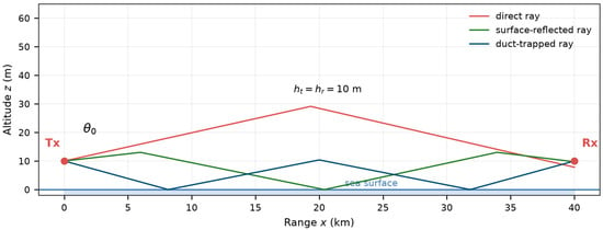
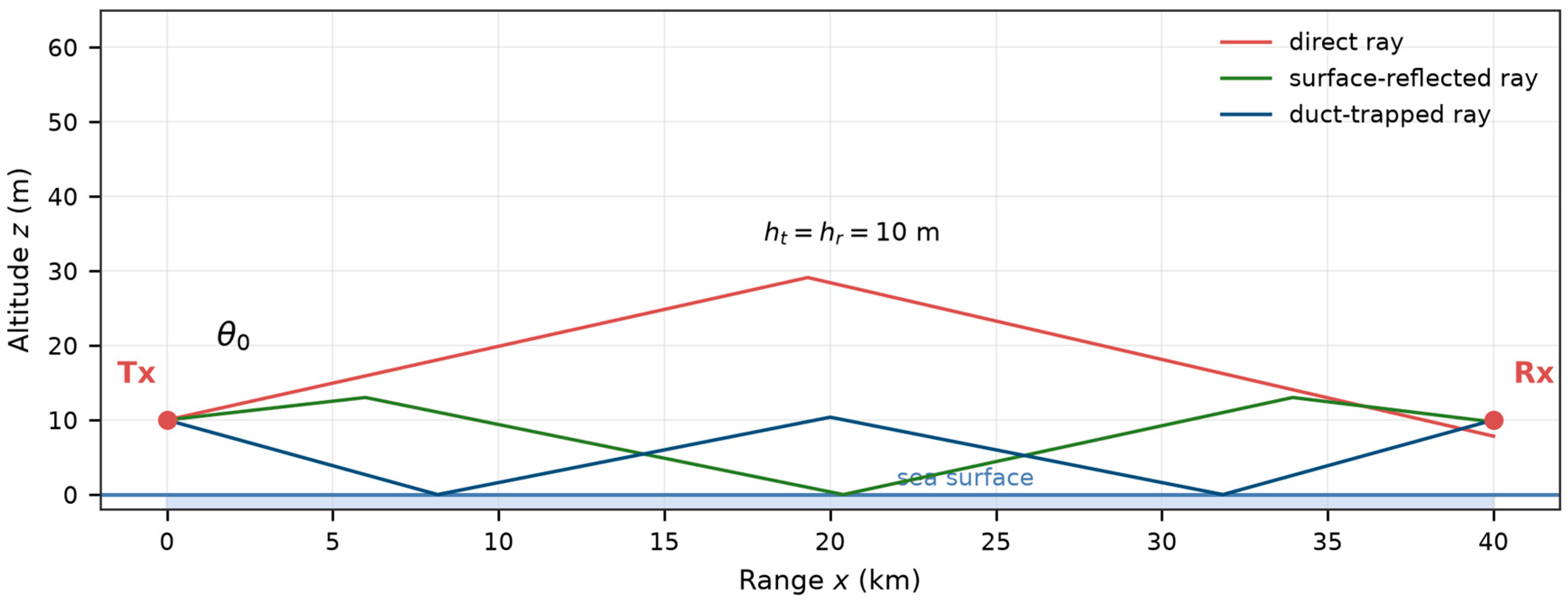
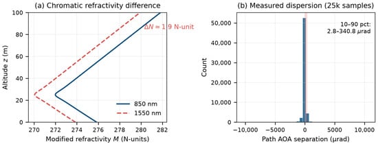
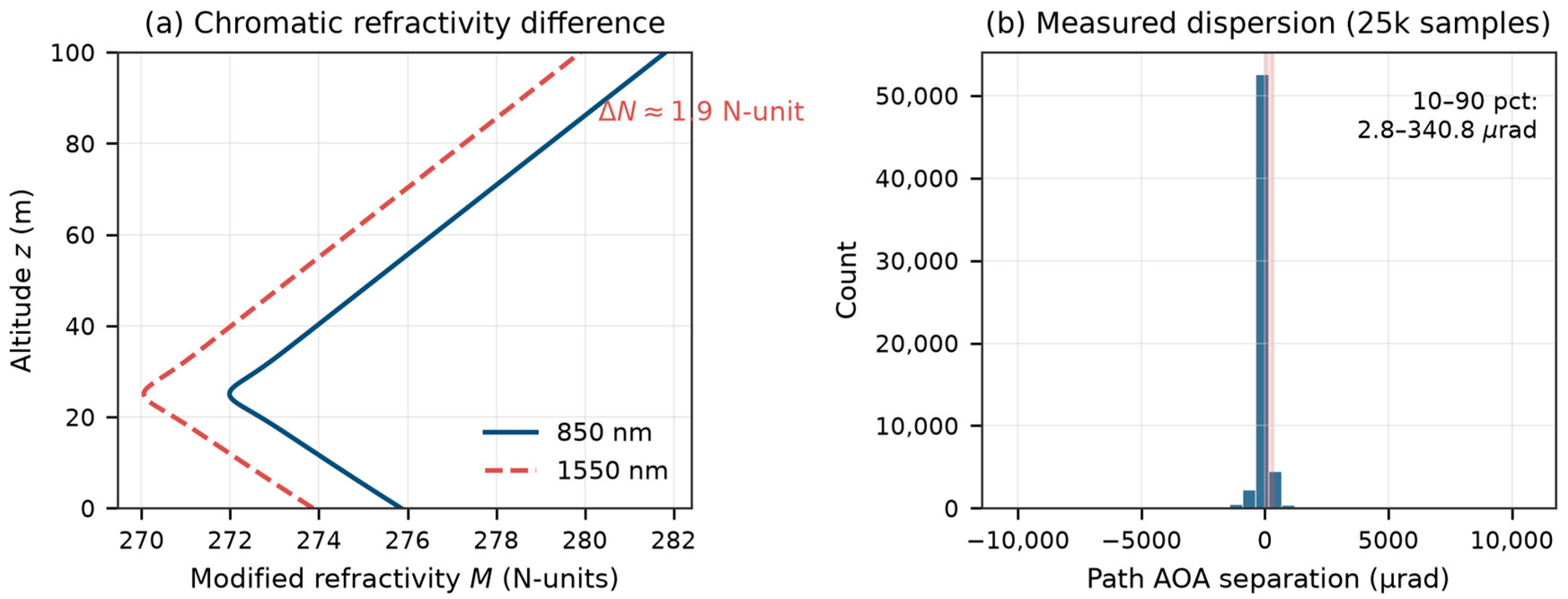
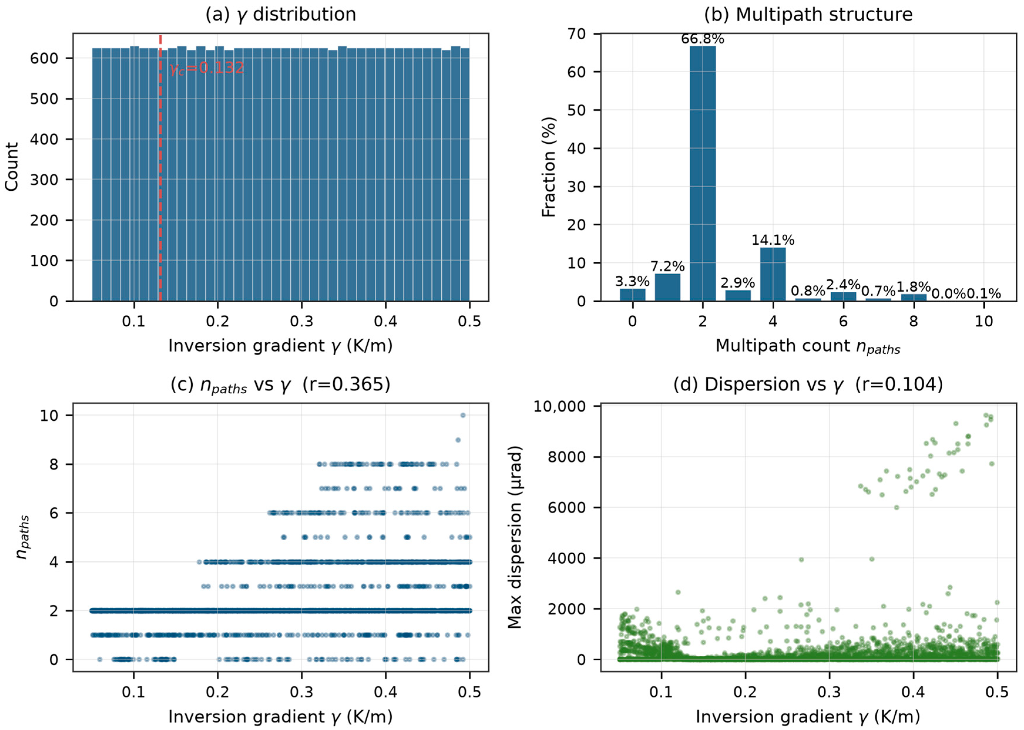
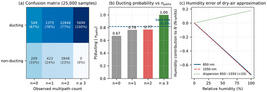
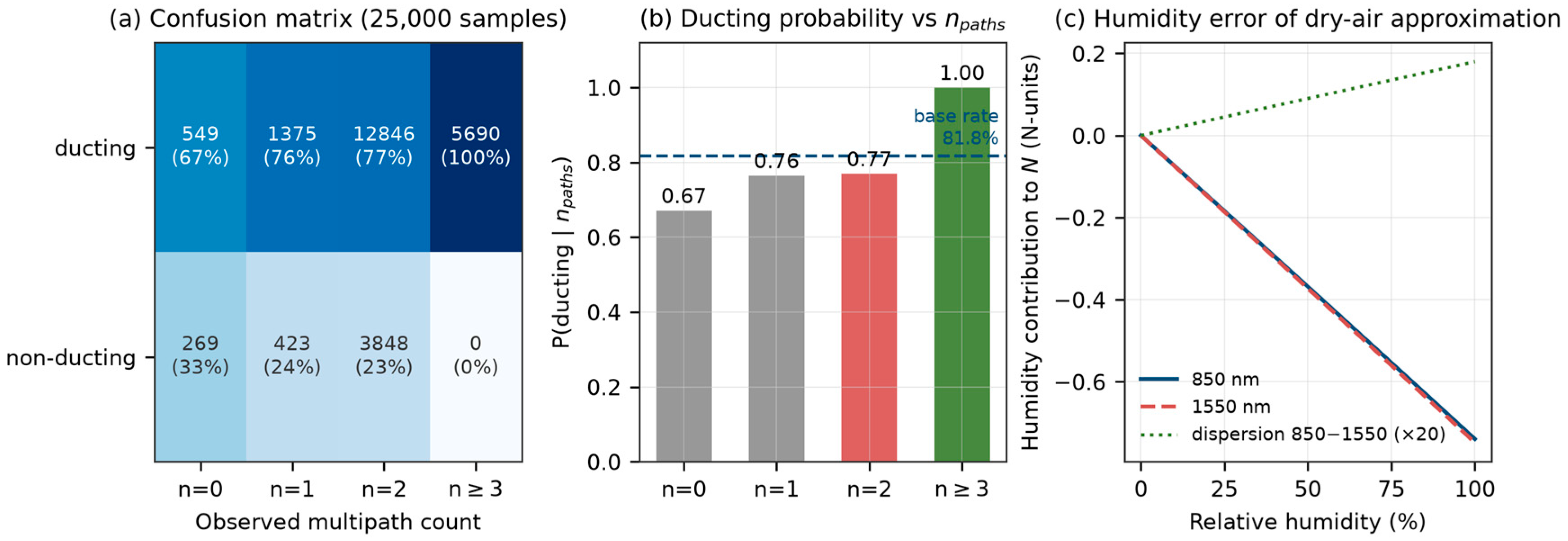
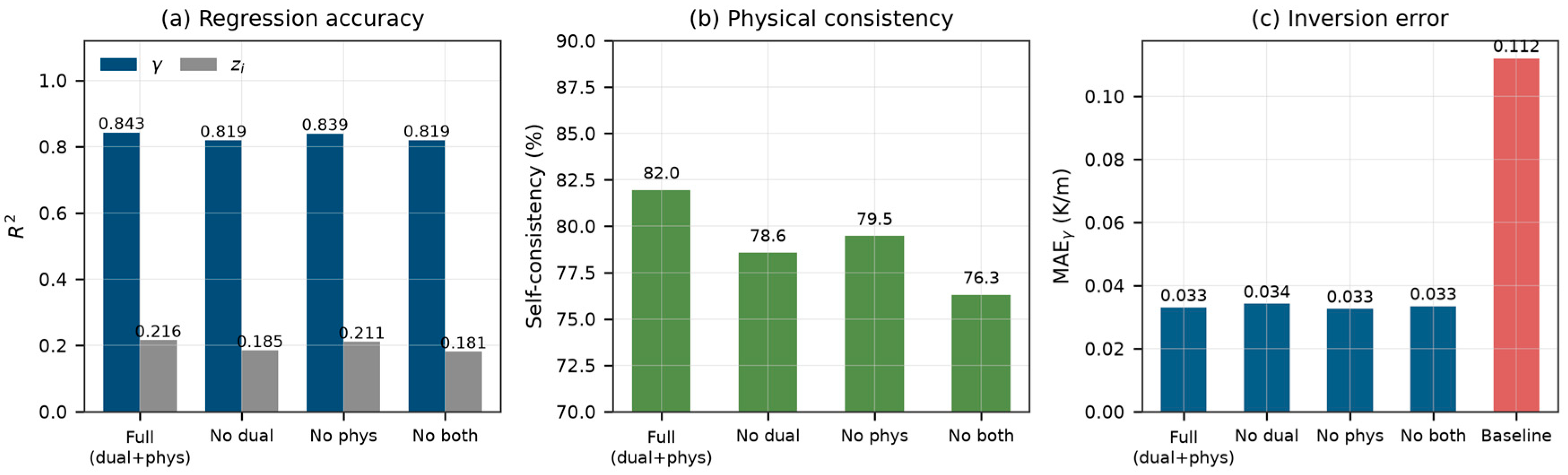
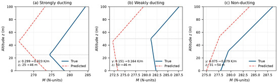
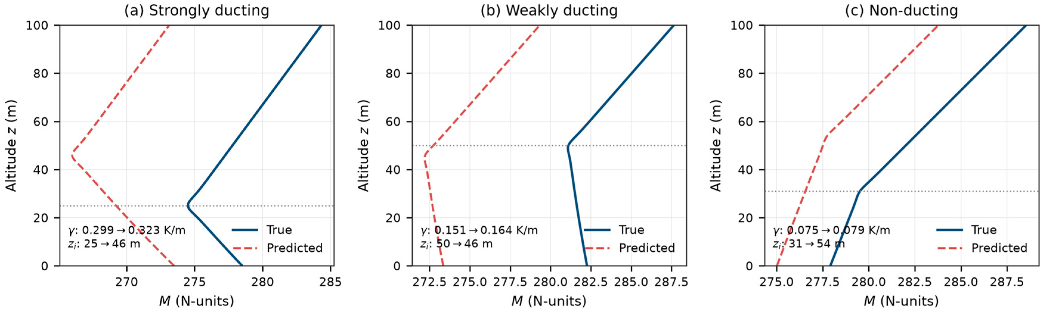
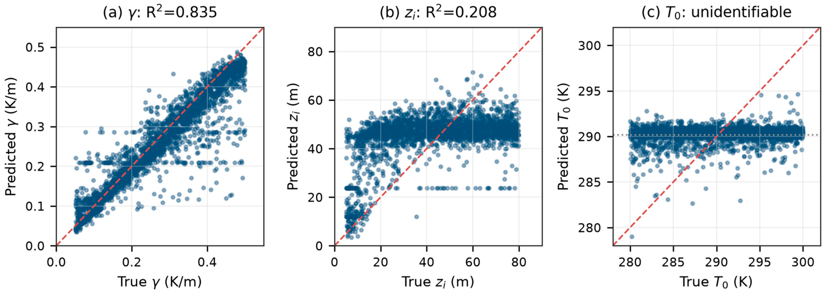
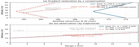
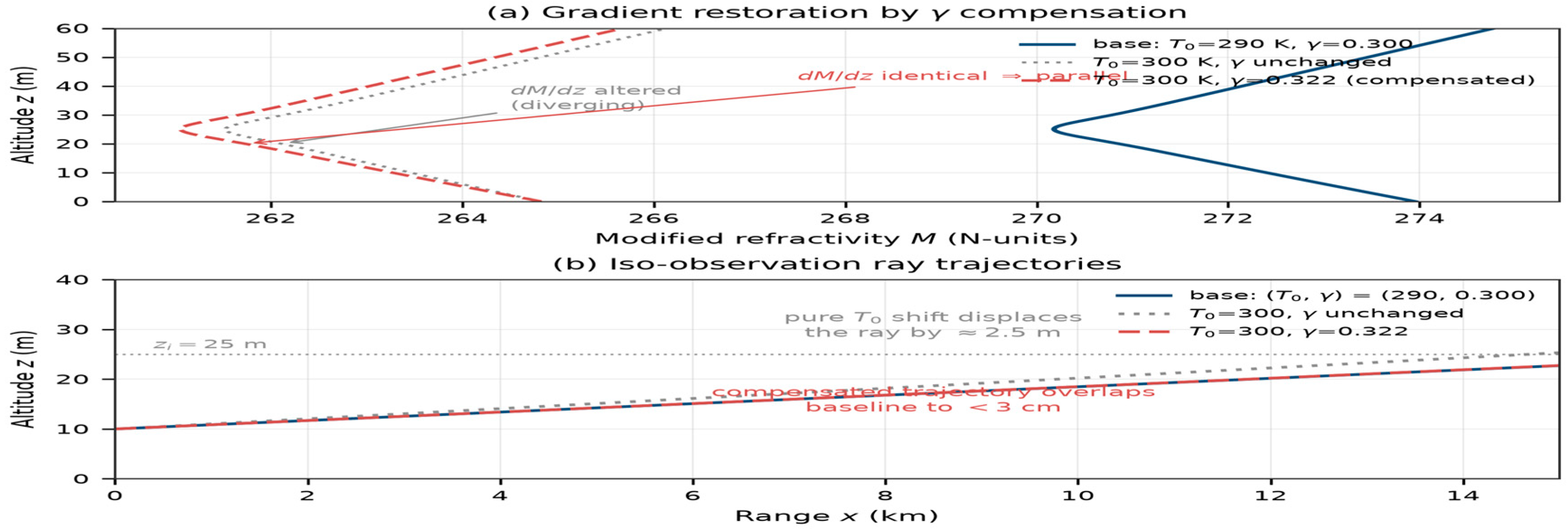
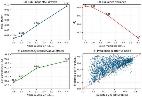
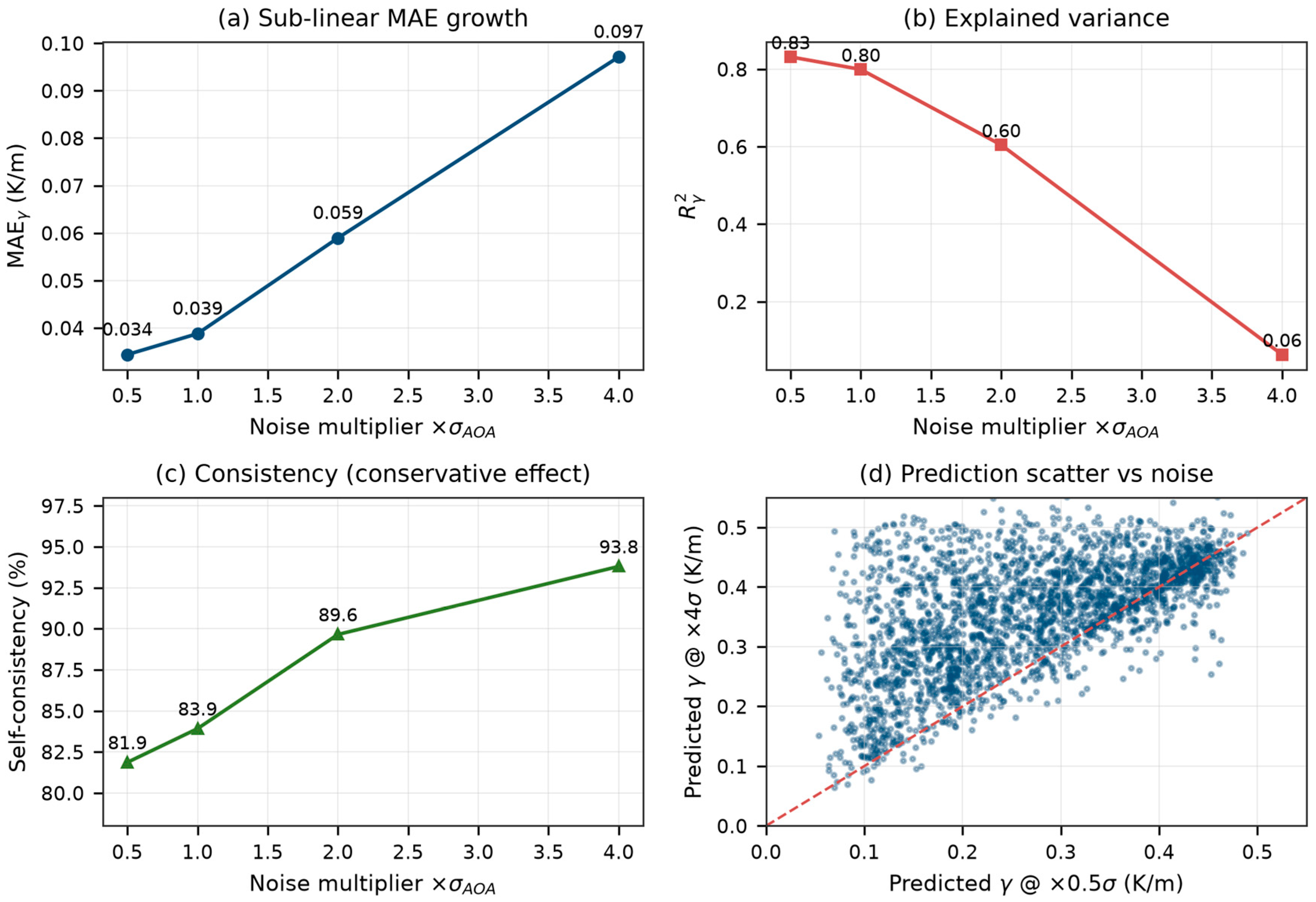

Disclaimer/Publisher’s Note: The statements, opinions and data contained in all publications are solely those of the individual author(s) and contributor(s) and not of MDPI and/or the editor(s). MDPI and/or the editor(s) disclaim responsibility for any injury to people or property resulting from any ideas, methods, instructions or products referred to in the content. |
© 2026 by the authors. Licensee MDPI, Basel, Switzerland. This article is an open access article distributed under the terms and conditions of the Creative Commons Attribution (CC BY) license.