


Abstract
This paper applies the Adomian decomposition method (ADM) to construct semi-analytical series solutions of linear and nonlinear time-fractional Klein–Gordon equations with the Caputo derivative (), and compares them with the homotopy perturbation method (HPM). Whereas previous ADM studies of this equation were restricted to linear problems, quadratic and cubic nonlinearities are treated here, and explicit recursive formulas are derived for the series components, whose coefficients depend on through gamma-function ratios. The convergence of the series and the stability of the solution with respect to the initial data are established. For the problems considered, ADM and HPM generate identical components term by term, as confirmed numerically to round-off. The seven-term approximations are assessed for , and 2 against exact or independent numerical reference solutions, using the and error norms, an error reduction index and the CPU time. They are highly accurate in the linear case and at short times in the nonlinear cases, and their accuracy improves as increases. In the nonlinear cases, however, the series converge only on a finite time interval that shrinks as decreases, which motivates multistage strategies such as Step-ADM for longer times.
Keywords:
time-fractional Klein–Gordon equation; homotopy perturbation method; Adomian decomposition method; fractional partial differential equations MSC:
35R11; 35Q40; 65M99; 26A33
1. Introduction
Fractional calculus extends the classical differential and integral operators to non-integer orders and provides powerful tools for modeling complex phenomena with memory effects and non-local properties. It has attracted considerable attention in many scientific disciplines because it can describe real-world processes more accurately than integer-order models [1,2].
The mathematical foundations of fractional calculus, laid by the pioneering work of Liouville and Riemann, have led to diverse applications in engineering, biology, control systems and viscoelastic materials [3]. In particular, fractional partial differential equations (FPDEs) have become essential tools for modeling phenomena in fluid mechanics, biological systems and quantum mechanics [4,5,6]. Recent studies of nonlinear fractional wave models, such as the M-fractional paraxial wave equation [7,8] and the M-fractional (3+1)-dimensional generalized B-type Kadomtsev–Petviashvili equation [9], illustrate the variety of nonlinear dynamics, including solitons and bifurcations, that such models can capture.
However, most FPDEs have no closed-form analytical solution, which calls for reliable approximation techniques [10,11]. This challenge has driven major advances along two parallel lines: numerical methods and theoretical analysis. On the numerical side, powerful techniques such as the reproducing kernel Hilbert space method, the Chelyshkov collocation method and finite difference methods have been developed to obtain accurate solutions of difficult problems [12,13,14,15,16,17,18,19]. Among semi-analytical approaches, the variational iteration method [20], the Adomian decomposition method () [21,22,23] and the homotopy perturbation method () [24,25,26,27,28,29,30,31] have demonstrated particular effectiveness. The , introduced by He [32], requires neither linearization nor the assumption of a small parameter, while the provides a systematic framework that typically converges rapidly. Hybrid forms of the that combine it with integral transforms have recently been applied to fractional models in the Caputo sense, including the Chafee–Infante equation [33], the Kawahara and modified Kawahara equations [34] and the sine-Gordon equation [35].
On the theoretical side, much research has focused on the qualitative analysis of fractional dynamical systems, including impulsive fractional differential equations and inclusions, which model systems subject to sudden changes. The controllability of such systems, that is, the ability to steer a system to a desired state, has also been studied extensively for various classes of fractional equations with state-dependent delay, non-instantaneous impulses and specific operators such as the -Hilfer derivative [36,37,38,39,40,41,42,43,44].
This work focuses on a specific and physically significant FPDE: the fractional-order Klein–Gordon equation. It generalizes the classical Klein–Gordon equation by replacing the integer-order time derivative with a fractional derivative of real order , with . Its general form is
where denotes the Caputo fractional derivative of order with respect to time, is the spatial Laplacian, m is a mass-related parameter and contains all the nonlinear terms.
Fractional derivatives introduce memory effects into the dynamics and thus allow a more realistic modeling of wave propagation in complex media. This formulation is particularly useful for describing physical phenomena in heterogeneous materials, fractal structures and systems with anomalous diffusion or non-local interactions. Because fractional operators are non-local, they are also well suited to quantum systems in which memory effects and long-range interactions play a fundamental role.
Following [45], we consider the fractional Klein–Gordon equation in the form
where and is a known source function, subject to the initial conditions
Previous studies have shown the usefulness of analytical methods for fractional Klein–Gordon equations. Golmankhaneh et al. [45] applied the to nonlinear fractional Klein–Gordon equations and obtained solutions consistent with classical results. Tamsir and Srivastava [46] showed that the fractional reduced differential transform method and the give consistent solutions. More recently, Albogami et al. [47] applied the to linear time-fractional Klein–Gordon equations and presented the approximate solutions numerically and graphically, and Sahu and Jena [48] solved the time-fractional Klein–Gordon equation with a modified Laplace–Adomian decomposition method hybridized with a Newton–Raphson scheme. Mannaf et al. [49] also investigated solitary-wave solutions of the fractional Klein–Gordon model. Collocation methods have also been developed for nonlinear Klein–Gordon equations, based on Hosoya polynomials [50], on Bernoulli wavelets [51] and, for the fractional case, on Fibonacci wavelets [52]. However, the treatment in [47] was limited to linear problems and, to the best of our knowledge, a direct comparison of and for nonlinear fractional Klein–Gordon equations, with explicit component formulas valid for every and validation against an independent numerical solution, has not been reported.
This gap motivates the present work, in which the is applied to linear and nonlinear (quadratic and cubic) time-fractional Klein–Gordon equations and the results are compared with those of the . The main contributions of this paper are as follows: (i) explicit recursive formulas for the series components, valid for every , which show that from the third component onwards the coefficients depend on through gamma-function ratios; (ii) convergence and stability results for the series solutions; (iii) an explanation of why, for polynomial nonlinearities, the and generate identical components, together with a numerical confirmation; and (iv) an assessment of the seven-term approximations against exact or independent numerical reference solutions, using the and error norms, an error reduction index and the CPU time, which reveals the finite convergence interval of the nonlinear series.
The paper is organized as follows. Section 2 recalls the necessary concepts of fractional calculus. Section 3 and Section 4 present the and the for the fractional Klein–Gordon equation, and Section 5 establishes the convergence and stability results. Section 6 presents three representative applications, Section 7 discusses the results and Section 8 concludes.
2. Preliminaries
This section recalls the basic concepts of fractional calculus used in this paper.
Definition 1
([2]). The Riemann–Liouville fractional integral operator of order of a function , continuous in x and y on , is defined by
Definition 2
([2]). The Caputo fractional derivative of order α of a function with respect to y is defined by for , and , and
Definition 3
([53]). The two-parameter Mittag–Leffler function is defined by When , and .
3. Adomian Decomposition Method for Nonlinear Klein–Gordon Equations
Consider the nonhomogeneous nonlinear fractional partial differential equation written in operator form [54]
where denotes the Caputo fractional derivative of order with , , L represents a linear operator, is a nonlinear operator, and is the source term.
Applying the fractional integral operator to both sides of Equation (5) and using the fact that the Caputo derivative of a constant is zero yields
for , with initial conditions for .
The unknown function is decomposed into the infinite series
The nonlinear term is expanded in Adomian polynomials ,
which are defined by
The first Adomian polynomials are
Substituting (7) and (8) into the integral Equation (6) gives
which leads to the recursive relations
The convergence of the Adomian decomposition method was established by Abbaoui and Cherruault [55]. In practice, a few terms of the series often give an accurate approximation, which can be improved by including further terms, provided that the series converges (see Section 7).
4. Homotopy Perturbation Method
4.1. Procedure of the Homotopy Perturbation Method
To illustrate the basic idea of the , consider the general differential equation [26]
subject to the boundary condition
where A is a general differential operator, B is a boundary operator, is a known analytic function and is the boundary of the domain .
Assume that the operator A can be split into a linear part L and a nonlinear part M, so that Equation (13) can be written as
The homotopy is constructed as
where is an initial approximation of the solution of Equation (13) and is the homotopy mapping.
4.2. Application to the Fractional Klein–Gordon Equation
For the nonlinear fractional Klein–Gordon Equation (2), we construct the homotopy
which is equivalent to
where the second term corresponds to the original equation
Here, is the homotopy parameter. For , Equation (18) reduces to
while for , Equations (18) and (19) are equivalent to the original Equation (2).
4.3. Series Solution and Recursive Scheme
The solution is expanded in powers of the homotopy parameter :
For the nonlinear term , we use He’s polynomials:
where are He’s polynomials [26]. Substituting (21) into (19) and equating the coefficients of like powers of yields the recursive system
The components are obtained by applying the fractional integral operator [45], and the solution of Equation (2) is then obtained by setting in the series.
5. Convergence and Stability Analysis in the Nonlinear Case
For the nonlinear time-fractional Klein–Gordon problem (2)–(4), we consider the Banach space of bounded uniformly continuous functions on , equipped with the supremum norm . With pointwise multiplication, X is a Banach algebra: . The operator , with domain , generates the strongly continuous cosine family , with , and so does its bounded perturbation [56], with for some and . With the nonlinear operator , the problem can be written in the abstract form
By the subordination principle ([57], Theorem 3.1), for the operator L generates an -times resolvent family with , where . Let and let for , with . These operators satisfy
and, for , the mild solution of (23) with the initial data and is given by [57]
5.1. Local Lipschitz Continuity of the Nonlinearity
Lemma 1.
For every , the nonlinear operator is locally Lipschitz continuous on :
where .
Proof.
Since and , the Banach algebra property gives . □
5.2. Convergence of and
Theorem 1.
Let , and let the components belong to . Assume that
- (i)
- there exist and such that for all and ;
- (ii)
- the series converges in X, uniformly on .
Then the following hold.
- (a)
- The series converges absolutely and uniformly on to a function .
- (b)
- For every , the truncation error satisfies
- (c)
- The sum ψ satisfies the integral equation on , and it coincides with the mild solution (25).
Proof.
(a) By (i), for and , where is finite because is continuous. Since , the Weierstrass M-test gives the absolute and uniform convergence, and the sum is continuous as a uniform limit of continuous functions.
(b) For and , (i) gives , so that .
(c) Let . Summing the recursive relations for gives
The series is b times the Cauchy product of with itself plus c times the threefold Cauchy product. Because X is a Banach algebra and converges uniformly on , Mertens’ theorem shows that uniformly on . By (ii) and the closedness of , and uniformly on . Finally, is bounded on , with . Letting therefore yields the integral equation in (c). A function in that satisfies this equation is a strong solution of (23), and hence a mild solution (25) [57]. The mild solution is unique: by Theorem 2 with identical initial data, two mild solutions bounded by R coincide. □
5.3. Nonlinear Stability Analysis
Theorem 2.
Let and be two mild solutions (25) in , bounded by R, corresponding to the initial data and and to the same source term g. Then there exists a constant , independent of the initial data, such that
Proof.
We use the following generalized fractional Gronwall inequality ([58], Corollary 2): let , let be a nonnegative, nondecreasing and locally integrable function on , let be a constant, and let be nonnegative and locally integrable on with
Then for .
Let and . Subtracting the mild formulations (25) of and , the source terms cancel, and
Since , Lemma 1 and the bounds (24) give, for ,
The function is continuous and nonnegative, so the Gronwall inequality applies with , the constant and . Since is increasing on , we obtain (27) with
In particular, implies , which proves the uniqueness of the mild solution among solutions bounded by R. □
Remark 1
(Effect of the Fractional Order). For the problems of Section 6, , so that, at a fixed x, the series is a power series in and condition (i) of Theorem 1 holds below a boundary . Since grows faster for larger α, increases with α and, for a fixed number of terms, the truncation error decreases faster, as observed in Section 7. In the linear case of Application 1, for , so that
with , and the series converges for all to ; in the nonlinear cases, grows rapidly with n and is finite.
Remark 2
(– Equivalence). For the polynomial nonlinearity , He’s polynomials, obtained from the expansion with respect to the embedding parameter ρ, coincide with the Adomian polynomials. The therefore generates the same components as the , for , and conclusions (a)–(c) of Theorem 1 also hold for the series. This equivalence is a property of the homotopy construction used here and should not be interpreted as a general identity between the two methods for all nonlinear problems.
6. Numerical Illustration
We consider three problems that were originally solved with the in [45]. For each of them, we derive the solution, compare it with the solution and assess both against an exact or reference solution; all computations and figures were produced in MATLAB R2014a.
- Application 1: Fractional Linear Homogeneous Klein–Gordon Equation
Setting , and in Equation (2) gives the fractional linear homogeneous Klein–Gordon equation, with the initial conditions
According to [45], the gives the following series components for this problem:
The exact solution is therefore
Since Equation (29) is linear, the yields the same series components, and hence the same semi-analytical solution, as the .
Comparative numerical results for and 2, computed at with terms of each series, are presented in Table 1, Table 2 and Table 3, respectively. At the grid points , , with , the absolute errors of the N-term approximations and with respect to the exact solution are defined by
and the column gives the absolute difference between the two approximations. The global error norms are
The error reduction index (ERI) at each grid point compares the errors of the -term and N-term approximations:
which is undefined when either error is zero to machine precision. The ERI is not an order of convergence in the usual sense: the number of terms N is not a discretization parameter, and the errors of series approximations decrease faster than any power of N. It measures how much the N-th term reduces the error at a given time; positive values mean that the error decreases, and negative values that it increases. A proper estimated order can be obtained by successive halving of t: since the truncation error of the N-term approximation is as , the observed order should approach , and we verified that it does so in all three applications. The exact solution is evaluated by summing its series up to , which gives machine precision over . All computations were performed in MATLAB, and the CPU time of each method was measured with the tic/toc functions.
Table 1.
Comparison of the exact solution and the and solutions for in Application 1 (, ). A dash indicates that the ERI is undefined because the error is zero to machine precision.
Table 2.
Comparison of the exact solution and the and solutions for in Application 1 (, ). A dash indicates that the ERI is undefined because the error is zero to machine precision.
Table 3.
Comparison of the exact solution and the and solutions for in Application 1 (, ). A dash indicates that the ERI is undefined because the error is zero to machine precision.
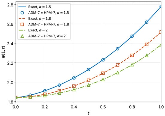
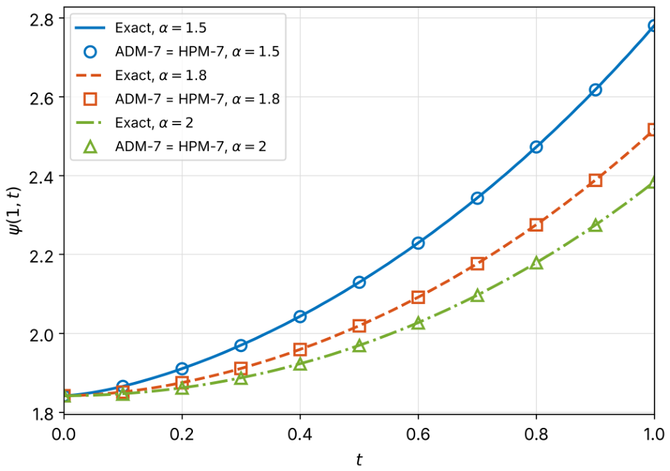
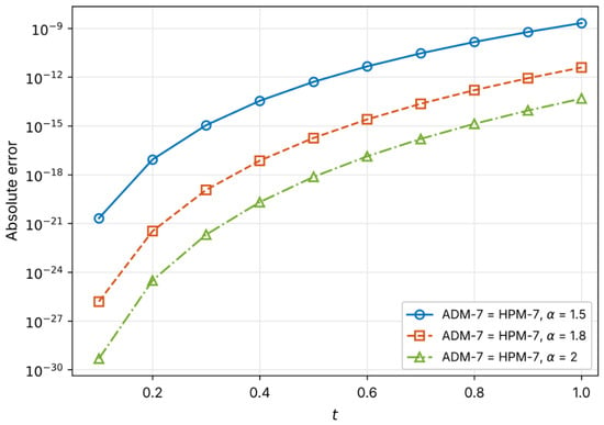
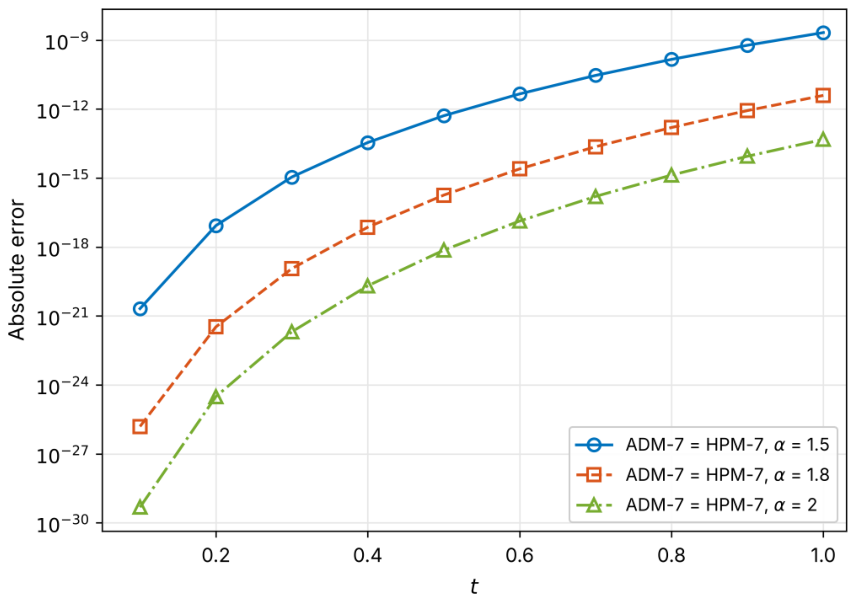
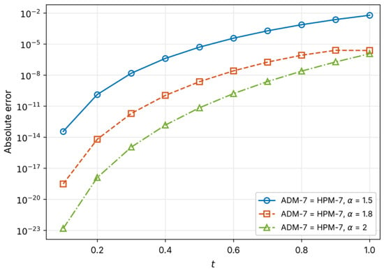
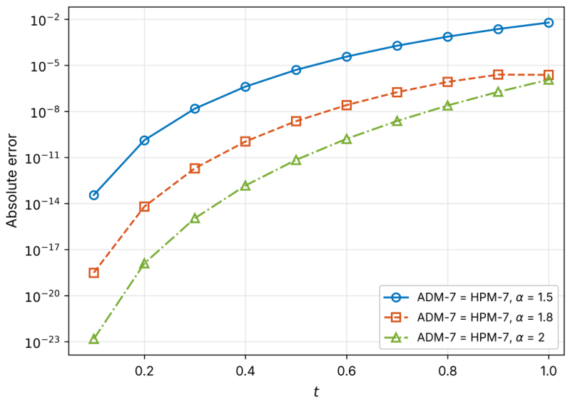
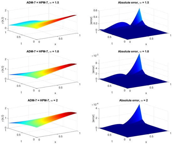
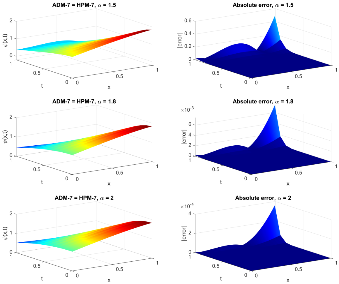
Table 4 summarizes the and error norms (31) over , together with the CPU time required by each method to evaluate its seven-term approximation on the time grid, for , and . Since Equation (29) is linear, the and approximations coincide term by term, and their errors are identical. With seven terms, both approximations reproduce the exact solution to within for , for and for ; the error decreases as increases because the factor grows faster. Figure 1 compares the exact solution with the seven-term approximations at , Figure 2 shows their absolute errors on a logarithmic scale, and Figure 3 shows the solution and absolute-error surfaces on .
Table 4.
Summary of the and error norms and CPU times for Application 1 (, ).
Figure 1.
Exact solution and seven-term (=) approximations at for Application 1.
Figure 3.
Exact and seven-term () solution surfaces (left) and absolute-error surfaces (right) for Application 1. The colour of each surface indicates its height, from dark blue (lowest values) to yellow (highest values).
- Application 2: Fractional Nonlinear Homogeneous Klein–Gordon Equation
Setting , and in Equation (2) gives the fractional nonlinear homogeneous Klein–Gordon equation, with the initial conditions
Since , the components of the series can be written as . The nonlinear term is expanded in the Adomian polynomials
and the recursive scheme (12) becomes
Writing and using , the first components are
where . For , and reduces to , which is the component reported in [45]. For , however, , so and all higher components depend on through the gamma-function ratios in (34). The components are computed from (34) in the same way.
In the , the nonlinear term is expanded with He’s polynomials , defined as the coefficients of in . For a polynomial nonlinearity these coincide with the Adomian polynomials, , so the two methods generate the same components term by term. In our implementation, the two recursions are coded independently, and the computed and approximations agree to round-off (see Table 5, Table 6 and Table 7).
Table 5.
Reference solution and seven-term and solutions for in Application 2 (, ). Reference values marked with * are from the numerical solution; the others are from the converged series.
Table 6.
Reference solution and seven-term and solutions for in Application 2 (, ). Reference values marked with * are from the numerical solution; the others are from the converged series.
Table 7.
Reference solution and seven-term and solutions for in Application 2 (, ). Reference values marked with * are from the numerical solution; the others are from the converged series.
Since no closed-form solution is available for Applications 2 and 3, the errors (30) are measured against a reference solution obtained independently of and . Where the series has converged (the terms , and are all below ), the reference is the 20-term series, and the error of the seven-term approximation is computed directly as the tail , which avoids cancellation. Elsewhere, the reference is the numerical solution of the equivalent Volterra integral equation , computed with the product-integration trapezoidal rule [59] and a Fourier spectral discretization in x, using step sizes and combined by Richardson extrapolation. Where both references are available, they agree to within . Table 5, Table 6 and Table 7 report the results at for , and 2, and Table 8 summarizes the error norms (31) and the CPU times, which are averages over 200 runs of each method.
Table 8.
Summary of the and error norms and CPU times for Application 2 (, ).
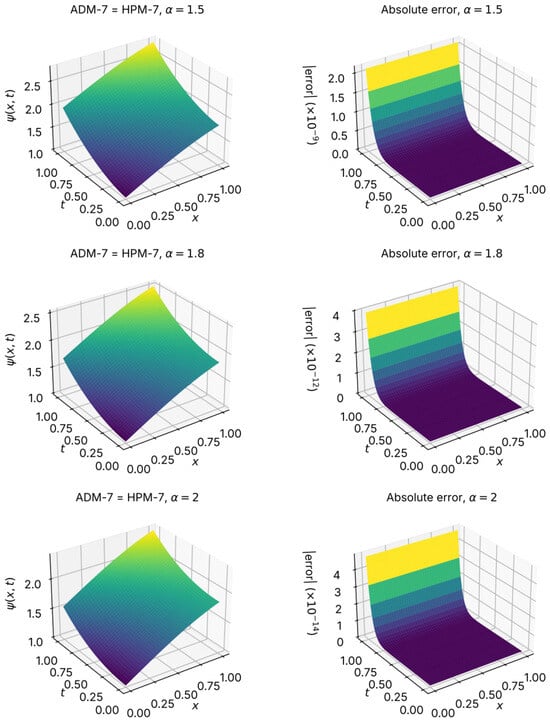
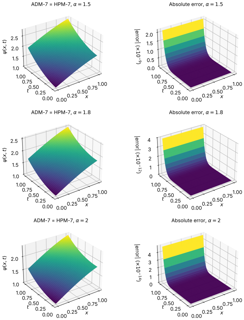
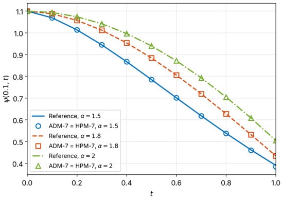
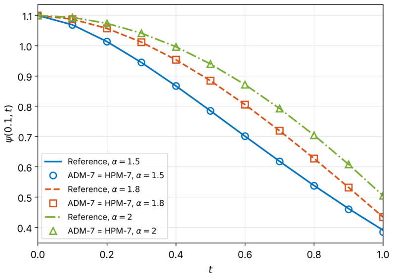
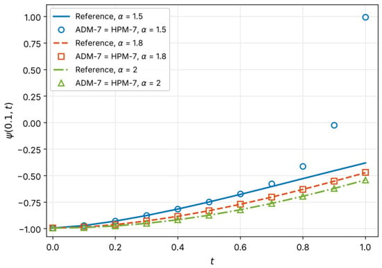
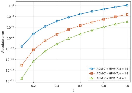
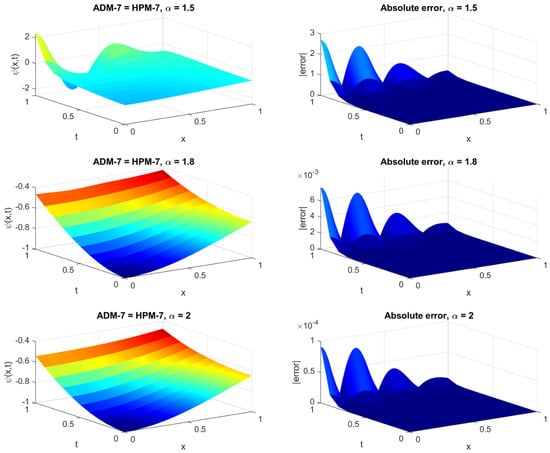
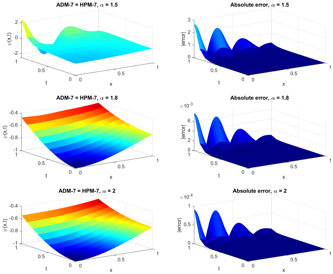
The seven-term and solutions coincide to round-off () for every value of . Their accuracy improves as increases: for , for and for . For , the error grows from at to at . On , this growth is a truncation effect: the series converges on the whole interval for all three values of , but for it converges slowly near , where more than seven terms are needed. The reference solution and the seven-term approximations at are compared in Figure 4, their absolute errors are shown in Figure 5, and the solution and absolute-error surfaces on are shown in Figure 6.
Figure 4.
Reference, and solutions at for Application 2.
Figure 5.
Absolute errors of and at for Application 2 (logarithmic scale).
Figure 6.
() solution surfaces (left) and absolute-error surfaces (right) on for Application 2.
- Application 3: Fractional Nonlinear Homogeneous Klein–Gordon Equation
Setting , and in Equation (2) gives a second fractional nonlinear homogeneous Klein–Gordon equation, with the initial conditions
The second initial condition, , is required because . As in Application 2, the components have the form . With the Adomian polynomials of the cubic term, , the recursive scheme reads
Writing and using , the first components are
with as in Application 2 (for , ). The components follow from (36); their coefficients also depend on . The first component can be checked directly: substituting into the right-hand side of (35) gives , which is . As in Application 2, He’s polynomials of the cubic term coincide with the Adomian polynomials, so the generates the same components.
The results at are reported in Table 9, Table 10 and Table 11, with the reference solution computed as in Application 2 (Fourier discretization on ); the error norms and CPU times are summarized in Table 12.
Table 9.
Reference solution and seven-term and solutions for in Application 3 (, ). Reference values marked with * are from the numerical solution; the others are from the converged series.
Table 10.
Reference solution and seven-term and solutions for in Application 3 (, ). Reference values marked with * are from the numerical solution; the others are from the converged series.
Table 11.
Reference solution and seven-term and solutions for in Application 3 (, ). Reference values marked with * are from the numerical solution; the others are from the converged series.
Table 12.
Summary of the and error norms and CPU times for Application 3 (, ).
For and , the seven-term approximations are accurate, with maximum errors of and ; the errors stay below up to for and up to for . For , the series converges only on a short interval (up to about ). The error is at , but it grows to at and to at , where the seven-term sum () no longer approximates the solution (). The negative ERI values for show that adding the seventh term increases the error there. This loss of accuracy is a property of the truncated series itself, shared by and , and not an instability of either scheme. It also explains why a higher-order truncated series, such as , cannot serve as a reference in this region: it diverges. Multistage strategies such as Step-, which restart the series on successive time intervals, are therefore needed to extend the approximation to longer times. The reference solution and the seven-term approximations at are compared in Figure 7, their absolute errors are shown in Figure 8, and the solution and absolute-error surfaces on are shown in Figure 9.
Figure 7.
Reference, and solutions at for Application 3.
Figure 8.
Absolute errors of and at for Application 3 (logarithmic scale).
Figure 9.
() solution surfaces (left) and absolute-error surfaces (right) on for Application 3. The colour of each surface indicates its height, from dark blue (lowest values) to yellow (highest values).
7. Results and Discussion
Agreement between and . In all three applications, the seven-term and approximations coincide: their difference never exceeds , which is round-off level (Table 1, Table 2 and Table 3, Table 5, Table 6 and Table 7 and Table 9, Table 10 and Table 11). For the linear problem of Application 1, both methods reduce to the same expansion of the Mittag–Leffler function. For the quadratic and cubic nonlinearities of Applications 2 and 3, He’s polynomials coincide with the Adomian polynomials, so the two recursions generate identical components term by term, as shown in (34) and (36). In line with Remark 2, this equivalence is a property of the homotopy construction used for polynomial nonlinearities; it should not be expected for every nonlinear problem. Consequently, the errors, error reduction indices and error norms of the two methods are identical, and the methods differ only in their computational organization.
Linear case. For Application 1, the exact solution is an entire function of t, and the truncation error of the seven-term approximation is governed by the factor . The maximum errors at are , and for , and 2 (Table 4), and the ERI values between 24 and 39 confirm the rapid decay of the successive terms. For , the exact solution reduces to , the solution of the classical integer-order equation.
Nonlinear cases and influence of . At short times, the nonlinear approximations are also very accurate: at the errors range from (, Application 3) to (, Application 2). The errors grow with t and decrease markedly as increases. The maximum errors at are , and in Application 2, and , and in Application 3, for , and 2 respectively (Table 8 and Table 12). This dependence on follows from Remark 1: the factor grows more slowly for smaller , so the higher-order components, whose coefficients grow rapidly with n, are damped less.
Finite convergence interval. Unlike the linear case, the nonlinear series converge only on a finite time interval, which shrinks as decreases. On , this restriction affects only Application 3: at , its series stops converging at about for and for , whereas the series of Application 2 converges on the whole interval for the three values of considered. Beyond this point, the seven-term sum can still be a useful approximation, but adding further terms makes it worse. This effect is most visible in Application 3 with : the error grows from at to at , and the ERI becomes negative for (Table 9, Figure 7). This is a limitation of truncated series solutions as such, shared by and , and not a numerical instability. For the same reason, a higher-order truncated series (for example, -12) cannot serve as a reference solution in this region; an independent numerical solution is required, as used here.
Spatial dependence of the error. The tables report the error at , but Figure 6 and Figure 9 show that the error varies with x. In Application 2 the largest errors over occur near and , where the initial profile is largest: about , and for , and 2. In Application 3 they occur near , where is largest: about , and . The oscillations of the error surfaces of Application 3 in x come from the high-degree polynomials in that make up the components .
Computational cost. Computing the seven components takes less than s for every case considered (Table 4, Table 8 and Table 12). Since the two methods produce the same components, the small differences in CPU time reflect the implementation rather than an intrinsic advantage of either method: our code recomputes the products of the truncated homotopy series at each order, whereas the code evaluates only the Adomian polynomial required at that order.
8. Conclusions
In this work, the Adomian decomposition method was applied to linear and nonlinear time-fractional Klein–Gordon equations with the Caputo derivative (), and the resulting series solutions were compared with those of the homotopy perturbation method. Explicit recursive formulas were derived for the series components of the quadratic and cubic problems, showing that from the third component onwards their coefficients depend on through gamma-function ratios. The convergence of the series and the stability of the solution with respect to the initial data were established, and all seven-term approximations were assessed against the exact solution or an independent numerical reference, using the and error norms, an error reduction index and the CPU time.
The main conclusions are as follows. First, for the linear equation and for the polynomial nonlinearities considered, and generate identical components term by term, and their numerical results agree to round-off. Second, the approximations are highly accurate in the linear case (errors between and ) and at short times in the nonlinear cases, and their accuracy improves markedly as increases; for the classical integer-order solutions are recovered. Third, in the nonlinear cases the series converge only on a finite time interval that shrinks as decreases, so that for the seven-term approximation of the cubic problem is no longer reliable beyond . Finally, the error depends on the spatial variable, being largest where the amplitude of the initial profile is largest.
These results indicate that the and the are efficient and, for polynomial nonlinearities, equivalent tools for fractional Klein–Gordon equations over short time intervals. Natural next steps for extending the approximations to longer times are multistage strategies such as Step-, which restart the series on successive time intervals, and Padé approximants. The comparison could also be extended to non-polynomial nonlinearities, for which the two methods need not coincide.
Supplementary Materials
The following supporting information can be downloaded at https://www.mdpi.com/article/10.3390/mca31060262/s1, Code S1: KG_App1.m, MATLAB code for Application 1, which generates Table 1, Table 2, Table 3 and Table 4 and Figure 1, Figure 2 and Figure 3; Code S2: KG_App2_App3.m, MATLAB code for Applications 2 and 3, which computes the ADM and HPM components, the independent reference solution, the errors, error reduction indices, error norms and CPU times, and generates Table 5, Table 6, Table 7, Table 8, Table 9, Table 10, Table 11 and Table 12 and Figure 4, Figure 5, Figure 6, Figure 7, Figure 8 and Figure 9. Both codes are compatible with MATLAB R2014a and later.
Author Contributions
Conceptualization, D.S. and M.B.; methodology, N.M.; software, M.B.; validation, N.M. and D.S.; formal analysis, M.B.; investigation, N.M.; writing original draft preparation, N.M.; writing review and editing, D.S.; visualization, D.S.; supervision, M.B. All authors have read and agreed to the published version of the manuscript.
Funding
This research received no external funding.
Institutional Review Board Statement
Not applicable.
Informed Consent Statement
Not applicable.
Data Availability Statement
All data are contained within the article. The MATLAB codes that reproduce all tables and figures are provided as Supplementary Materials (Codes S1 and S2).
Conflicts of Interest
The authors declare no conflicts of interest.
References
- Kilbas, A.A.; Srivastava, H.M.; Trujillo, J.J. Theory and Applications of Fractional Differential Equations; Elsevier: Amsterdam, The Netherlands, 2006. [Google Scholar]
- Podlubny, I. Fractional Differential Equations; Academic Press: San Diego, CA, USA; Boston, MA, USA, 1999; Volume 6. [Google Scholar]
- Diethelm, K. Fast solution methods for fractional differential equations in the modeling of viscoelastic materials. In Proceedings of the 2021 9th International Conference on Systems and Control (ICSC), Caen, France, 24–26 November 2021; IEEE: New York, NY, USA, 2021; pp. 455–460. [Google Scholar] [CrossRef] [Scilit]
- Gul, H.; Alrabaiah, H.; Ali, S.; Shah, K.; Muhammad, S. Computation of solution to fractional order partial reaction diffusion equations. J. Adv. Res. 2021, 25, 31–38. [Google Scholar] [CrossRef] [Scilit] [PubMed]
- Schneider, W.R.; Wyss, W. Fractional diffusion and wave equations. J. Math. Phys. 1989, 30, 134–144. [Google Scholar] [CrossRef] [Scilit]
- Wang, F.; Ali, S.N.; Ahmad, I.; Ahmad, H.; Alam, K.M.; Thounthong, P. Solution of Burgers’ equation appears in fluid mechanics by multistage optimal homotopy asymptotic method. Therm. Sci. 2022, 26, 815–821. [Google Scholar] [CrossRef] [Scilit]
- Bashar, M.H.; Lee, S.; Ghosh, S.; Rahman, M.M. Dynamical exploration of optical soliton solutions for M-fractional paraxial wave equation. PLoS ONE 2024, 19, e0299573. [Google Scholar] [CrossRef] [Scilit] [PubMed]
- Bashar, M.H.; Mannaf, M.A.; Rahman, M.M.; Khatun, M.T. Optical soliton solutions of the M-fractional paraxial wave equation. Sci. Rep. 2025, 15, 1416. [Google Scholar] [CrossRef] [Scilit] [PubMed]
- Bashar, M.H.; Mannaf, M.A.; Rahman, A.; Islam, M.S.; Mawa, H.Z.; Akter, P. Exploration of soliton solutions and bifurcation analysis in fluid dynamics governed by M fractional (3+1)-dimensional generalized B-type Kadomtsev–Petviashvili (gBKP) equation. Eng. Rep. 2026, 8, e70642. [Google Scholar] [CrossRef] [Scilit]
- Cherruault, Y. Modèles et Méthodes Mathématiques pour les Sciences du Vivant; Presses Universitaires de France: Paris, France, 1998. [Google Scholar]
- Momani, S.; Odibat, Z. Numerical comparison of methods for solving linear differential equations of fractional order. Chaos Solitons Fractals 2007, 31, 1248–1255. [Google Scholar] [CrossRef] [Scilit]
- Ardabili, J.S.; Talaei, Y. Chelyshkov Collocation Method for Solving theTwo-Dimensional Fredholm–Volterra Integral Equations. Int. J. Appl. Comput. Math. 2018, 4, 25. [Google Scholar] [CrossRef] [Scilit]
- Atangana, A.; Araz, S.İ. New Numerical Scheme with Newton Polynomial: Theory, Methods, and Applications; Elsevier: London, UK, 2021. [Google Scholar] [CrossRef] [Scilit]
- Attia, N.; Akgül, A.; Seba, D.; Nour, A.; Riaz, M.B. Reproducing kernel Hilbert space method for solving fractal fractional differential equations. Results Phys. 2023, 35, 105225. [Google Scholar] [CrossRef] [Scilit]
- Attia, N.; Akgül, A.; Seba, D.; Nour, A. Reproducing kernel Hilbert space method for the numerical solutions of fractional cancer tumor models. Math. Meth. Appl. Sci. 2021, 46, 7632–7653. [Google Scholar] [CrossRef] [Scilit]
- Chandhini, G.; Prashanthi, K.S.; Antony Vijesh, V. Direct and integrated radial functions based quasilinearization schemes for nonlinear fractional differential equations. BIT Numer. Math. 2020, 60, 31–65. [Google Scholar] [CrossRef] [Scilit]
- Darzi, R.; Agheli, B. Analytical Approach to Solving Fractional Partial Differential Equation by Optimal q-Homotopy Analysis Method. Numer. Anal. Appl. 2018, 11, 134–145. [Google Scholar] [CrossRef] [Scilit]
- Li, C.; Zeng, F. Finite difference methods for fractional differential equations. Int. J. Bifurc. Chaos 2012, 22, 1230014. [Google Scholar] [CrossRef] [Scilit]
- Zhang, X.; Cao, J. A high order numerical method for solving Caputo nonlinear fractional ordinary differential equations. AIMS Math. 2021, 6, 13187–13209. [Google Scholar] [CrossRef] [Scilit]
- Ahmad, H.; Khan, T.A.; Yao, S.W. An efficient approach for the numerical solution of fifth-order KdV equations. Open Math. 2020, 18, 738–748. [Google Scholar] [CrossRef] [Scilit]
- Adomian, G. Solution of physical problems by decomposition. Comput. Math. Appl. 1980, 6, 279–291. [Google Scholar] [CrossRef] [Scilit]
- Li, C.; Wang, Y. Numerical algorithm based on Adomian decomposition for fractional differential equations. Comput. Math. Appl. 2009, 57, 1672–1681. [Google Scholar] [CrossRef] [Scilit]
- Odibat, Z.; Momani, S. Numerical methods for nonlinear partial differential equations of fractional order. Appl. Math. Model. 2008, 32, 28–39. [Google Scholar] [CrossRef] [Scilit]
- Dehghan, M.; Manafian, J.; Saadatmandi, A. Solving nonlinear fractional partial differential equations using the homotopy analysis method. Numer. Methods Partial. Differ. Equ. 2010, 26, 448–479. [Google Scholar] [CrossRef] [Scilit]
- He, J.-H. A coupling method of a homotopy technique and a perturbation technique for non-linear problems. Int. J. Nonlinear Mech. 2000, 35, 37–43. [Google Scholar] [CrossRef] [Scilit]
- He, J.-H. Some asymptotic methods for strongly nonlinear equations. Int. J. Mod. Phys. B 2006, 20, 1141–1199. [Google Scholar] [CrossRef] [Scilit]
- Jafari, H.; Seifi, S. Solving a system of nonlinear fractional partial differential equations using homotopy analysis method. Commun. Nonlinear Sci. Numer. Simul. 2009, 14, 1962–1969. [Google Scholar] [CrossRef] [Scilit]
- Maitama, S.; Zhao, W. Homotopy Perturbation Shehu Transform Method for Solving Fractional Models Arising in Applied Sciences. J. Appl. Math. Comput. Mech. 2021, 20, 71–82. [Google Scholar] [CrossRef] [Scilit]
- Rafiullah, M. A fifth-order iterative method for solving nonlinear equations. Numer. Anal. Appl. 2011, 4, 239–243. [Google Scholar] [CrossRef] [Scilit]
- Sajid, S.; Martínez, F.; Kaabar, M.K.A.; Samei, M.E. A novel Elzaki transform homotopy perturbation method for solving time-fractional non-linear partial differential equations. Bound. Value Probl. 2022, 2022, 91. [Google Scholar] [CrossRef] [Scilit]
- Zhao, X.E.; Chen, L.Q.; Hao, W.; Zhao, Y. Bifurcation Analysis Reveals Solution Structures of Phase Field Models. Commun. Appl. Math. Comput. 2024, 6, 64–-89. [Google Scholar] [CrossRef] [Scilit]
- He, J.-H. Homotopy perturbation technique. Comput. Methods Appl. Mech. Eng. 1999, 178, 257–262. [Google Scholar] [CrossRef] [Scilit]
- Nayak, S.K.; Jena, S.R. Efficient hybrid approach for time-fractional (1+1)-dimensional Chafee–Infante equation using the Shehu–Adomian decomposition method in the Caputo environment. J. Supercomput. 2026, 82, 437. [Google Scholar] [CrossRef] [Scilit]
- Sahu, I.; Jena, S.R. Numerical computation of fractional Kawahara and modified Kawahara equations in Caputo sense on integral transforms. J. Supercomput. 2025, 81, 752. [Google Scholar] [CrossRef] [Scilit]
- Jena, S.R.; Sahu, I. Approximate and analytical solution of sine–Gordon equation based on Laplace Adomian decomposition method. Int. J. Syst. Assur. Eng. Manag. 2025, 16, 914–926. [Google Scholar] [CrossRef] [Scilit]
- Agarwal, R.; Almeida, R.; Hristova, S.; O’Regan, D. Non-Instantaneous Impulsive Fractional Differential Equations with State Dependent Delay and Practical Stability. Acta Math. Sci. 2021, 41, 1699–1718. [Google Scholar] [CrossRef] [Scilit]
- Aimene, D.; Seba, D.; Laoubi, K. Controllability of impulsive fractional functional evolution equations with infinite state-dependent delay in Banach spaces. Math. Meth. Appl. Sci. 2021, 44, 7979–7994. [Google Scholar] [CrossRef] [Scilit]
- Boudjerida, A.; Seba, D.; N’Guérékata, G.M. Controllability of coupled systems for impulsive φ-Hilfer fractional integro-differential inclusions. Appl. Anal. 2020, 101, 383–400. [Google Scholar] [CrossRef] [Scilit]
- Boudjerida, A.; Seba, D. Approximate controllability of hybrid Hilfer fractional differential inclusions with non-instantaneous impulses. Chaos Solitons Fractals 2021, 150, 111125. [Google Scholar] [CrossRef] [Scilit]
- Boudjerida, A.; Seba, D. Controllability of nonlocal Hilfer fractional delay dynamic inclusions with non-instantaneous impulses and non-dense domain. Int. J. Dyn. Control 2022, 10, 1613–1625. [Google Scholar] [CrossRef] [Scilit]
- Benchohra, M.; Seba, D. Integral equations of fractional order with multiple time delays in Banach spaces. Electron. J. Differ. Equ. 2012, 2012, 1–8. [Google Scholar] [CrossRef] [Scilit]
- Boudjerida, A.; Seba, D.; Meskine, N.; Benghanem, M. Oscillation of non-instantaneous impulsive hybrid-fractional delay differential inclusions with Hilfer-Katugampola derivative. J. Appl. Math. Comput. 2025, 71, 6749–6771. [Google Scholar] [CrossRef] [Scilit]
- Seba, D. A Comparative Analysis of Methodologies for Oscillation Theory in Parabolic Partial Differential Equations. Islam. Univ. J. Appl. Sci. 2025, VII, 150–164. [Google Scholar] [CrossRef] [Scilit]
- Zhou, Y. Fractional Diffusion and Wave Equations: Well-Posedness and Inverse Problems; Springer: Berlin/Heidelberg, Germany, 2024. [Google Scholar] [CrossRef] [Scilit]
- Alireza, K.G.; Golmankhaneh, A.K.; Baleanu, D. On nonlinear fractional Klein–Gordon equation. Signal Process. 2011, 91, 446–451. [Google Scholar] [CrossRef] [Scilit]
- Tamsir, M.; Srivastava, V.K. Analytical study of time-fractional order Klein–Gordon equation. Alex. Eng. J. 2016, 55, 561–567. [Google Scholar] [CrossRef] [Scilit]
- Albogami, D.; Maturi, D.; Alshehri, H. Adomian decomposition method for solving fractional time-Klein–Gordon equations using Maple. Appl. Math. 2023, 14, 411–418. [Google Scholar] [CrossRef]
- Sahu, I.; Jena, S.R. An efficient technique for time fractional Klein–Gordon equation based on modified Laplace Adomian decomposition technique via hybridized Newton–Raphson scheme arises in relativistic fractional quantum mechanics. Partial Differ. Equ. Appl. Math. 2024, 10, 100744. [Google Scholar] [CrossRef] [Scilit]
- Mannaf, M.A.; Jannah, M.; Bashar, M.H.; Islam, M.E.; Rana, M.Z.; Khatun, M.T.; Siddiki, M.N.-A.-A.; Islam, M.S. Exploring nonlinear dynamics and solitary waves in the fractional Klein–Gordon model. Adv. Math. Phys. 2025, 2025, 9970003. [Google Scholar] [CrossRef] [Scilit]
- Nirmala, A.N.; Kumbinarasaiah, S. Numerical solution of nonlinear Hunter–Saxton equation, Benjamin–Bona–Mahony equation, and Klein–Gordon equation using Hosoya polynomial method. Results Control Optim. 2024, 14, 100388. [Google Scholar] [CrossRef] [Scilit]
- Kumbinarasaiah, S.; Mulimani, M. Bernoulli wavelets numerical approach for the nonlinear Klein–Gordon and Benjamin–Bona–Mahony equation. Int. J. Appl. Comput. Math. 2023, 9, 108. [Google Scholar] [CrossRef] [Scilit]
- Mulimani, M.; Kumbinarasaiah, S. A numerical study on the nonlinear fractional Klein–Gordon equation. J. Umm Al-Qura Univ. Appl. Sci. 2024, 10, 178–199. [Google Scholar] [CrossRef] [Scilit]
- Aimene, D.; Baleanu, D.; Seba, D. Controllability of semilinear impulsive Atangana–Baleanu fractional differential equations with delay. Chaos Solitons Fractals 2019, 128, 1–7. [Google Scholar] [CrossRef] [Scilit]
- Wazwaz, A.M. Partial Differential Equations and Solitary Waves Theory; Higher Education Press: Beijing, China; Springer: Berlin/Heidelberg, Germany, 2009. [Google Scholar] [CrossRef] [Scilit]
- Abbaoui, K.; Cherruault, Y. New ideas for proving convergence of decomposition methods. Comput. Math. Appl. 1995, 29, 103–108. [Google Scholar] [CrossRef] [Scilit]
- Arendt, W.; Batty, C.J.K.; Hieber, M.; Neubrander, F. Vector-Valued Laplace Transforms and Cauchy Problems, 2nd ed.; Birkhäuser: Basel, Switzerland, 2011. [Google Scholar] [CrossRef] [Scilit]
- Bajlekova, E.G. Fractional Evolution Equations in Banach Spaces. Ph.D. Thesis, Eindhoven University of Technology, Eindhoven, The Netherlands, 2001. [Google Scholar]
- Ye, H.; Gao, J.; Ding, Y. A generalized Gronwall inequality and its application to a fractional differential equation. J. Math. Anal. Appl. 2007, 328, 1075–1081. [Google Scholar] [CrossRef] [Scilit]
- Garrappa, R. Numerical solution of fractional differential equations: A survey and a software tutorial. Mathematics 2018, 6, 16. [Google Scholar] [CrossRef] [Scilit]

Disclaimer/Publisher’s Note: The statements, opinions and data contained in all publications are solely those of the individual author(s) and contributor(s) and not of MDPI and/or the editor(s). MDPI and/or the editor(s) disclaim responsibility for any injury to people or property resulting from any ideas, methods, instructions or products referred to in the content. |
© 2026 by the authors. Licensee MDPI, Basel, Switzerland. This article is an open access article distributed under the terms and conditions of the Creative Commons Attribution (CC BY) license.