


Abstract
This study develops an analytical inverse framework for estimating the effective area of a single leak at a known location in a horizontal gas pipeline. A one-dimensional isothermal diffusion model with constant resistance and separately parameterised boundary pressures is coupled with compressible discharge. Modal and Volterra representations describe pressure and leakage under choked conditions. Independent finite-difference verification gives a pressure root-mean-square discrepancy of 0.011 Pa in the finest benchmark comparison. Extended Monte Carlo tests cover four pressure-noise levels and three opening diameters; at 10 Pa noise, relative area root-mean-square errors are 11.61%, 2.90%, and 0.73% for 10, 20, and 40 mm openings, respectively. Location and resistance errors produce additional estimation bias. Across three leak positions, a 10-fold leakage increase requires area increases of 10.076–10.211 times because of local pressure feedback. However, a nonlinear-friction benchmark yields approximately 1.00 kPa pressure discrepancy and drives absolute-pressure inversion to the zero-area bound. The results establish numerical consistency and conditional sensitivity while revealing substantial model discrepancy. Geometric-area recovery requires discharge-coefficient calibration, and operational application requires further model assessment and experimental validation.
1. Introduction
Natural gas pipeline systems are critical components of modern energy infrastructure, and their safe operation depends strongly on the preservation of pipeline integrity. A local loss of tightness may cause gas to escape into the surrounding environment, reduce the delivery capacity of the pipeline, and create significant operational, economic, and safety risks. In addition to detecting and locating a leak, it is important to estimate the size of the damaged section. An estimate of equivalent leak area may provide supplementary information for preliminary damage assessment. Its use in repair planning requires independent inspection, discharge-characteristic calibration, and validation of the hydraulic model; the equivalent area alone does not determine repair duration or the expected interruption of gas supply. Neglecting convective acceleration at low Mach numbers, approximating wall friction by a linear resistance, and neglecting local inertia relative to friction yield the diffusion-type pressure model used here. For relatively small gas velocities, the convective acceleration term can be neglected, and the governing equations can be linearised. This leads to diffusion-type pressure equations that are suitable for analytical treatment and numerical verification. Gugat et al. investigated analytical and numerical solutions of transient gas pipeline flow and compared them with quasi-static approximations [1]. Related studies have considered the operation and optimisation of transient gas-transport networks [2]. These investigations demonstrate the importance of transient modelling for describing the temporal evolution of pressure and flow in gas pipelines.
The authors’ previous studies provide a direct basis for the present research. Mammadov, Mammadrzayeva, and Aliyev developed an analytical and asymptotic model of coupled transient gas redistribution caused by simultaneous injection and withdrawal in transmission pipelines [3]. Their results showed that time-dependent sources and sinks produce measurable pressure redistribution along the pipeline and can be represented within a linearised compressible-flow framework. Aliyev investigated unsteady gas dynamics in relief-influenced pipelines and developed a pressure-inversion procedure for interpreting transient hydraulic behaviour [4]. These studies established the analytical basis for using transient pressure data not only for forward prediction but also for inverse identification of pipeline disturbances.
A substantial body of research has focused on leak detection and localisation. Mechanistic models based on inlet and outlet pressure and flow measurements have been developed for identifying leak-related hydraulic responses [5]. Transient matched-field processing has been used to compare measured pressure signals with modelled pressure fields and to estimate leak-related parameters [6]. Other studies have analysed the first transient pressure wave while accounting for unsteady friction effects [7]. More recently, dynamic gas pipeline models have been combined with machine-learning methods to estimate leak location and leakage magnitude [8]. Optimisation-based approaches have also been experimentally verified in pipeline systems containing branches and diameter changes [9].
Time-dependent pressure and leakage representations provide a useful basis for interpreting gas-release transients. Dutton and Coverdill [10] derived analytical solutions for gas discharge from vessels, including exponential pressure decay under isothermal, choked-flow conditions. Although this result concerns a spatially uniform vessel, it provides a physical motivation for considering exponential approximations over suitable depressurisation intervals. In a pipeline context, Aliyev et al. [11] developed an analytical framework for leakage detection in parallel pipelines using a time-dependent leakage mass-flow representation linked to inlet-pressure information. Building on these approaches, the present study adopts independently parameterised inlet and outlet pressure histories and couples the local pressure to compressible discharge to estimate the equivalent leak area at a known location.
Although these studies have significantly advanced leak detection and localisation, the direct determination of the geometric size of a damaged section remains comparatively less developed. In many existing approaches, leakage magnitude is represented by a fitted coefficient, a classified severity level, or an equivalent hydraulic parameter. Such representations may indicate the intensity of a leak, but they do not necessarily provide emergency personnel with a physically interpretable estimate of the opening area. Furthermore, a number of models use simplified boundary conditions, such as constant pressure, constant flow rate, or a common pressure-decay coefficient at both ends of the pipeline. These assumptions may be unsuitable when the inlet and outlet pressure histories evolve differently during a transient event.
The present study addresses this problem by developing an analytical inverse framework for estimating the equivalent leak area of a gas pipeline from transient pressure and flow data. A one-dimensional isothermal compressible-flow model is formulated for a horizontal pipeline, with frictional resistance included and gravitational effects neglected. The leakage point is represented as a localised hydraulic junction, and the pressure histories at the inlet and outlet are described independently by the decay coefficients βg and βs. The local leakage discharge is coupled to the pressure at the damaged section, allowing the effective hydraulic area to be related directly to the equivalent geometric opening area.
The proposed analytical solution is verified independently using a finite-difference method. In addition, the influence of leakage severity is investigated for several leakage-flow ratios, namely Qle/Q0 = 0.1, 0.3, 0.5, 0.8, and 1.0. This analysis establishes the relationship between the leakage-flow rate, local pressure, equivalent opening area, and equivalent diameter. The study therefore extends conventional leak-detection research from the identification of a leak and its position to the quantitative estimation of the physical scale of the damaged section.
The main contributions of this study are as follows:
- An analytical transient model is developed for a gas pipeline containing a localised leakage point.
- Independently varying inlet and outlet pressure-decay coefficients, βg and βs, are incorporated into the boundary conditions.
- A pressure–discharge coupling relation is introduced to determine the equivalent leak area from the local transient pressure and leakage flow.
- The analytical solution is verified against an independent finite-difference solution.
- A parametric analysis is performed to quantify the relationship between leakage-flow severity and the geometric dimensions of the damaged section.
The resulting framework provides an analytical basis for investigating the information about effective leak areas contained in transient pressure observations. Its potential contribution to emergency assessment remains conditional on model adequacy, parameter calibration, and experimental validation.
Literature Review
Transient gas pipeline modelling provides the foundation for interpreting pressure redistribution and estimating hydraulic parameters from observations. Gugat et al. [1] presented analytical examples and numerical simulations of transient gas flow and examined their relationship to quasi-static approximations. Hoppmann-Baum et al. [2] investigated the optimal operation of transient gas-transport networks, demonstrating the role of mathematical flow models in operational decision-making. These studies establish relevant forward-modelling approaches, although their principal objectives differ from the inverse estimation of a local leak opening.
Related analytical developments underpin the present formulation. Mammadov, Mammadrzayeva, and Aliyev [3] investigated coupled transient gas redistribution induced by simultaneous injection and withdrawal in transmission pipelines. Their treatment of distributed pressure responses to sources and sinks supports the representation of leakage as a localised mass withdrawal. Aliyev [4] subsequently considered unsteady gas dynamics in relief-influenced pipelines and developed a pressure-inversion formulation. These contributions provide methodological continuity for the present study, which neglects elevation effects and treats the constant effective area of a leak at a known location as the unknown parameter.
Previous leakage studies have addressed both localisation and size estimation. Kam [5] developed a mechanistic model under a fixed inlet-rate condition and examined changes in inlet pressure and outlet flow as functions of leak opening size and longitudinal position. Wang and Ghidaoui [6] formulated a transient matched-field-processing method for estimating leak location and size from pressure responses, including cases affected by measurement noise and uncertainty in wave speed. These studies demonstrate that hydraulic observations can contain information about opening size, as well as location. Accordingly, leak-size estimation itself cannot be regarded as an unexplored problem.
Other investigations have developed complementary approaches to transient leakage diagnosis. Diao et al. [7] analysed the first transient pressure wave in liquid pipelines while accounting for unsteady friction. Kim et al. [8] combined dynamic gas pipeline modelling with machine learning to estimate leak size and location under transient conditions. Asada et al. [9] reported field verification of an optimisation-based transient-pressure method in an irrigation pipeline containing branch junctions and diameter changes. These contributions differ in their physical assumptions, observation requirements, and estimation procedures. In particular, wave-based methods for liquid pipelines and simulation-trained gas pipeline methods provide relevant comparisons, but their results do not directly establish the validity of a diffusion approximation for gas-pressure dynamics.
The representation of boundary-pressure evolution also requires a distinction between physical motivation and an imposed modelling assumption. Dutton and Coverdill [10] derived vessel-discharge solutions that include exponential pressure decay under isothermal, choked-flow conditions. Their analysis motivates an exponential approximation over suitable intervals but does not establish that the boundaries of a distributed pipeline must follow the same law. Aliyev et al. [11] developed an analytical leakage framework for parallel pipelines using a time-dependent leakage representation linked to pressure information. In the present study, inlet and outlet pressure histories are parameterised independently. For measured records, the suitability of these representations must be assessed by fitting the observations and examining the residuals; the numerical examples use prescribed synthetic histories.
Against this background, the present contribution is an analytical formulation linking transient pressure observations to a constant effective opening area at a known leak location. Local compressible discharge is coupled to a diffusion-type gas-pressure model, yielding explicit series representations for pressure and leakage under choked conditions. The unknown effective area is estimated by fitting the predicted pressure response to independent interior observations. Conversion to geometric opening area requires an independently specified discharge coefficient; the hydraulic response alone does not identify the area and discharge coefficient separately.
Recent studies have explicitly addressed leakage quantification alongside detection and localisation. Li et al. [12] developed a transformer-based framework for simultaneous leakage-aperture recognition and localisation in gas pipelines under noisy conditions. Ebrahimi et al. [13] proposed a deep-learning framework for detecting, locating, and estimating leakage rates in gas networks with variable supply and consumption, including noise augmentation during training. These contributions establish that leak-size and leakage-rate estimation are active research topics. Accordingly, the contribution of the present study is the analytical formulation of effective-area inversion within a specified reduced-order gas-flow model, rather than the introduction of leak-size estimation as a new objective.
Inverse leakage estimation has also been investigated using observations outside the pipeline. Zhao et al. [14] combined a modified Gaussian plume model with Bayesian inference and Markov chain Monte Carlo sampling to estimate leakage location and rate from methane-concentration information. Their analysis considered the influence of systematic errors and highlighted the importance of reliable forward modelling, monitoring data, and prior information. Although concentration-based source estimation differs from the internal-pressure inversion considered here, it provides a relevant methodological perspective: the reliability of inferred leakage parameters depends on both observational uncertainty and the adequacy of the forward model.
High-fidelity numerical investigations further demonstrate the importance of the discharge assumptions. Xia et al. [15] developed coupled numerical models of transient gas flow and leakage diffusion and examined the factors governing leakage rates. Their results indicated that neglecting boundary-layer effects and spatial variations in the gas state can overestimate leakage, while discrepancies between ideal- and real-gas predictions increase with pressure. These findings motivate careful assessment of the simplified discharge closure used in the present framework. The analytical model provides a tractable relationship between pressure response and effective opening area, but its physical accuracy remains conditional on the adopted flow assumptions and discharge-coefficient calibration.
Taken together, the reviewed studies demonstrate substantial progress in transient modelling, leak localisation, aperture recognition, and leakage-rate estimation. The present study contributes an analytical formulation for estimating a constant effective opening area at a known leak location, using a diffusion-type pressure model with separately parameterised boundary histories and local pressure–discharge coupling. The pressure and leakage histories are represented through modal and Volterra formulations, providing an explicit mathematical basis for the inverse calculation. The distinction between effective and geometric opening areas is retained throughout: conversion to geometric area requires an independently specified discharge coefficient. Numerical verification and sensitivity analyses assess performance within the stated assumptions, while model discrepancy and the absence of experimental validation limit claims concerning operational accuracy.
Table 1 compares representative transient-flow and leakage-estimation approaches in terms of their modelling assumptions, estimation targets, and relevance to the present study. The comparison identifies prior contributions to leak localisation and size estimation and clarifies the specific scope of the proposed framework: analytical inversion of an effective opening area at a known location, conditional on the adopted diffusion model and discharge relation.
Table 1.
Comparative analysis of representative transient-flow and leakage-estimation approaches and the proposed leak-area inversion framework.
2. Mathematical Model and Problem Formulation
A loss of gas pipeline integrity alters the gas inventory, pressure distribution, and relationship between inlet and outlet mass flow rates. Quantifying these changes provides a physical basis for estimating the equivalent area of a leak opening from observations. This study considers a leak at a known location and focuses on estimating its area. The opening area is assumed constant over the observation interval, whereas the leakage mass flow rate varies with the local pressure. This formulation links the transient gas response to a geometric measure of the damage.
Consider a horizontal pipeline of length L, internal diameter d, and constant cross-sectional area F = πd2/4. Elevation effects are neglected. The axial coordinate is x ∈ [0,L], and time is denoted by t. The absolute pressure, density, and mean axial velocity are denoted by P(x,t), ρ(x,t), and v(x,t), respectively. The mass flow rate is defined as Q(x,t) = Fρv and is expressed in kg/s. The flow is assumed to be one-dimensional and isothermal. With constant temperature and compressibility factor, the equation of state becomes
Here, Z is the compressibility factor, Rs is the specific gas constant, T is the absolute temperature, and c is the characteristic speed associated with the pressure–density relation in the adopted isothermal model. Under the constant-Z approximation, c2 = (∂P/∂ρ)T = P/ρ. This parameter is distinguished from the local adiabatic speed of sound governing sonic discharge through the leak opening.
Away from the leak, gas motion is governed by mass and momentum conservation. For a horizontal pipe with wall friction, the isothermal governing equations are [1,2]
The parameter λ is the Darcy friction factor, and denotes the leak location. The axial flow is assumed to satisfy |v|/c≪1. For sufficiently smooth flow in this regime, the convective momentum term is neglected. This approximation does not itself linearize the friction term. To obtain a linear model, the velocity magnitude in that term is replaced by a reference value |v∗| [4]. The resistance parameter is defined by 2a = λ|v∗|/(2d), where a has units of s−1. The resulting pressure–mass-flow system is
An analytical diffusion approximation is obtained by considering a regime in which local inertia is small relative to friction. For a characteristic variation time τ, the condition 2aτ≫1 expresses the corresponding temporal scale separation. The momentum equation then reduces to
This reduction does not resolve the rapid wave response immediately following leak initiation. Its application interval must therefore be selected with regard to the initial acoustic transient and the rate of change of the boundary conditions. The accuracy of the constant-resistance approximation also depends on departures from the reference velocity.
The constant-resistance closure is obtained by freezing the velocity magnitude in the Darcy friction term at a reference value. It should therefore be distinguished from a first-order perturbation model of nonlinear friction. For positive mass flow at fixed local pressure, the nonlinear resistance in the mass-flow momentum equation is proportional to Q2. Its derivative at the reference flow is twice that of a linear resistance selected to reproduce the same friction magnitude at that point. Consequently, matching the initial steady through-flow does not necessarily reproduce the transient pressure sensitivity to leakage. The influence of this distinction on area estimation is examined through an additional nonlinear-friction benchmark in Section 4.
The leak is represented as a localized mass sink at . Defining Qle(t) ≥ 0 as the outward leakage mass flow rate and extending the continuity equation to include this sink yields, together with Equation (5),
Here, δ is the Dirac delta distribution and D is the diffusion coefficient, with units of m2/s. Additional localized pressure losses at the leak junction are neglected. Under this assumption, pressure remains continuous, whereas mass flow exhibits a jump:
The associated pressure-gradient jump is
Equations (7) and (8) provide the equivalent interface formulation of the point-sink representation in Equation (6).
The initial state is taken as the steady flow immediately before leak initiation. If the initial inlet and outlet pressures are Pg0 and Ps0, respectively, the adopted linear resistance model gives
The inlet and outlet pressure histories are represented by separate exponential functions over a selected observation interval. This representation is a tractable approximation to the boundary observations, rather than a universal consequence of pipeline leakage. In an operating network, boundary pressures may also respond to compressor operation, pressure regulation, changes in supply and demand, and interactions with connected pipelines. Consequently, a leakage event does not generally produce an exact exponential pressure decay at either endpoint.
A physical example of exponential depressurisation is provided by the isothermal discharge of an ideal gas from a fixed-volume vessel through a choked opening [10]. Under these assumptions, both stored mass and discharge rate are proportional to pressure, yielding a constant relative pressure-decay rate. However, this lumped-vessel result does not establish the same behaviour at the boundaries of a distributed pipeline. The time-dependent leakage modelling considered by Aliyev et al. [11] provides related methodological context but does not remove the need to assess the selected boundary representation against observations.
The two decay coefficients are estimated separately without imposing their equality. This does not imply statistical independence or physical decoupling of the inlet and outlet pressures. Both histories may be influenced by common network disturbances. Separate parameterisation simply allows their observed decay rates to differ; equality or inequality of the fitted coefficients does not, by itself, determine the leak location.
For measured records, the exponential approximation should be assessed by fitting the pressure histories over the selected interval and examining the magnitude and temporal structure of the residuals. The fitting interval should exclude abrupt operating changes unless they are explicitly represented. If substantial systematic departures remain, measured boundary histories or a more flexible representation should be used. In the present numerical study, the exponential histories are prescribed synthetic inputs and are not claimed to be experimentally established pressure responses.
Here, Pg0 and Ps0 are the absolute boundary pressures at t = 0.
The parameters βg and βs, expressed in s−1, characterize the relative decay rates of the corresponding boundary pressures. They are estimated separately, without imposing equality, and are not constrained to be equal. The exponential representation is restricted to the observation interval and is not extrapolated to the entire depressurization process. The local leak pressure must remain above atmospheric pressure for the outward-discharge formulation to apply. For exact exponential data,
For measured data, the decay parameters are estimated by fitting the full-time series rather than using a single observation. When pressure errors have approximately constant variance in absolute units, the exponential functions are fitted directly to the pressure observations by least squares. The boundary histories are thus informed by observations without imposing a predetermined relationship between their decay rates and the leak location.
Because pressure is prescribed through Equation (10), inlet and outlet mass flow rates are not imposed as additional boundary conditions. Instead, they follow from the boundary pressure gradients:
where flow measurements are available, they can be incorporated as additional observations in the inverse problem or used for validation. Exponential decay of the boundary pressure does not, in general, imply exponential decay of the boundary mass flow rate with the same coefficient.
Integrating the continuity equation over the pipeline relates leakage to the change in gas inventory:
Consequently, the inlet–outlet flow imbalance need not equal the leakage mass flow rate during a transient. Depletion of the gas stored in the pipe can also supply the leak. An estimate based on the flow imbalance must therefore account for the temporal evolution of the pressure field.
The relationship between leakage mass flow rate and opening area is expressed in the general form
Here, Fle is the geometric opening area, Cd is the discharge coefficient, Patm is atmospheric pressure, and Φ is the mass flux per unit area specified by the compressible discharge law. Gas properties enter as parameters of this function. The appropriate choked or unchoked expression is selected according to the pressure ratio. Although the opening area is constant, Equation (14) allows the leakage mass flow rate to evolve with the local pressure.
The inverse problem seeks to estimate the unknown area from internal pressure observations, given the boundary pressure histories and the known leak location. The two pressure histories used as boundary conditions do not alone determine the area; internal pressure or additional flow observations are required. If the discharge coefficient is not independently known, the parameter entering Equation (14) is the effective area Aeff = CdFle. Recovery of the geometric area therefore requires a known or calibrated discharge coefficient. The equivalent circular diameter is calculated as ; this measure does not separately resolve the length and width of an irregular crack.
3. Analytical Solution and Inverse Estimation of Leak Area
The analytical formulation is developed in two steps. First, the pressure field is obtained for a prescribed leakage mass-flow history. Subsequently, the leakage discharge is coupled with the local pressure through the opening-area relation. This distinction separates the solution of the pressure equation from the closure required to determine the leakage history. The leak location, , is assumed as being known, whereas the constant effective opening area is the parameter to be estimated.
To accommodate the independently varying boundary pressures, the pressure is decomposed as
where
The function B(x,t) satisfies the prescribed boundary conditions and coincides with the initial linear pressure distribution at t = 0. Consequently, substitution into Equation (6) gives
with
The residual pressure is expanded in a Fourier sine series:
Multiplying Equation (16a) by 2sin(knx)/L and integrating over the pipeline yields
The boundary-forcing coefficients follow from
and
Define the function
Application of the integrating-factor method to Equation (18) gives
and
The exponential boundary histories permit explicit evaluation of the boundary-forcing integrals but are not essential to the underlying solution construction. For sufficiently regular histories pg(t) and ps(t), the same boundary lifting and sine expansion apply, with modal forcing proportional to −[pg′(t) − (−1)nps′(t)]. The corresponding forcing integrals can be evaluated numerically. Thus, the framework can accommodate non-exponential boundary observations, although the explicit exponential expressions must then be replaced by the appropriate convolution integrals. Noisy boundary measurements require suitable fitting or smoothing before this derivative-based representation is used.
Substitution of Equation (20b) into Equation (17), followed by Equation (15a), gives the complete pressure representation:
Let P(0)(x,t) denote the pressure obtained from Equation (21) by setting Qle ≡ 0 while retaining the same initial and boundary conditions. Equation (21) separates the pressure response into the imposed boundary interpolation, the transient correction associated with gas storage, and the pressure reduction caused by leakage. The sine terms vanish at both endpoints, and H(μ,β,0) = 0; therefore, the prescribed boundary and initial conditions are satisfied directly. No equality between βg and βs is required.
Introduce the Dirichlet heat kernel
The pressure field can then be written as
This kernel representation is equivalent to Equation (21). Its interpretation is distributional at the leak: pressure is continuous, while its spatial derivative has the jump specified by Equation (8). In particular, the leak does not introduce pressure discontinuity in the adopted junction model.
To determine the leakage history, define the effective area θ = CdFle and the local pressure . The discharge relation is
For the ideal-gas closure, with r = Patm/p and γ > 1 [10],
where
Evaluating Equation (22b) at and substituting into Equation (23a) yields a closed equation for the leakage mass-flow history:
Equation (24) accounts for the feedback between leakage and local pressure. It determines Qle(t) for a specified trial area; substitution into Equation (21) then determines the complete pressure field. When the discharge changes between choked and unchoked conditions, the appropriate branch of Equation (23b) must be used throughout the solution.
For an observation interval during which discharge remains choked and temperature is constant, the mass flux is linear in pressure:
Let
Equation (24) then reduces to the linear Volterra equation
An explicit analytical representation follows through successive convolution. Define
The leakage history is
The complete iterated-integral expansion of Equation (25c) is
Here, the integration domain is 0 ≤ τm ≤ ⋯ ≤ τ1 ≤ t. For m = 1, the empty product is defined as unity, and the corresponding term is . For any finite observation interval 0 ≤ t ≤ Tobs, the diagonal heat kernel satisfies 0 ≤ K(t) ≤ Ct−1/2 for t > 0, with a suitable constant C. Consequently,
This bound establishes absolute and uniform convergence of Equation (25c) on finite time intervals for finite η. The convergent series solves Equation (25b), whose continuous solution is unique. Convergence does not, however, guarantee efficient numerical evaluation by direct summation; the coupled modal formulation or a suitable Volterra quadrature may be used in computation.
All quantities entering this representation are explicitly specified by
and
Thus, Equation (25d) expresses the leakage mass-flow rate entirely in terms of the specified pipeline parameters, boundary-pressure histories, leak location, and trial opening area. No unknown pressure or leakage function remains on its right-hand side. The representation applies over intervals of exclusively choked discharge with constant temperature and effective opening area.
Substitution of Equation (25c) into Equation (22b) gives a pressure representation containing no unknown leakage history:
Equations (25c) and (25e) provide the analytical leakage and pressure responses for a specified effective area under exclusively choked discharge. Their physical applicability requires verification that throughout the selected interval.
The leakage rate can also be recovered from the one-sided pressure gradients:
This expression follows directly from the interface mass balance and provides a consistency relation for the reconstructed pressure field. The derivatives must be interpreted as one-sided traces of the continuum solution. A finite sine expansion has a continuous derivative and therefore cannot reproduce the gradient jump by direct evaluation on its two sides at the same point.
For choked discharge, the geometric area is related to the reconstructed quantities by
Equation (25g) provides a direct area estimate when the leakage mass flow and local pressure are independently available. When both quantities are generated by the forward model for a trial area, the relation is an identity and does not independently determine the unknown parameter. The effective area is therefore estimated by fitting the predicted pressure field to independent interior observations.
Let yij denote the absolute pressure measured at the interior sensor location xi ∈ (0,L) and observation time tj, where i = 1,…, M and j = 1,…, N. Here, M is the number of sensors, N is the number of observation times, and σij > 0 is the standard deviation assigned to the corresponding measurement error. With the leak location, boundary histories, and remaining model parameters treated as known, the effective opening area is estimated by weighted least squares:
The upper bound is selected from physically admissible opening sizes and the range over which the reduced flow model remains applicable. When calibrated uncertainty estimates are unavailable, equal weights can be used. Boundary pressure observations are used to estimate βg and βs and impose Equation (10); they are not counted again as independent evidence for the leak area. Additional mass-flow observations, when available, can be incorporated with their own uncertainty weights. The scalar, constant-area formulation reduces the number of unknowns compared with reconstructing an arbitrary leakage history but does not remove sensitivity to boundary errors, friction, or gas-property uncertainty.
Local sensitivity to the effective area can be assessed without assigning a separate leakage value at every time step. Let S(x,t) = ∂P(x,t;θ)/∂θ. Differentiation of the coupled pressure equation gives, on a differentiable discharge branch,
Under choked discharge and , so the sensitivity equation remains linear in S for a fixed trial value of θ.
For independent, zero-mean Gaussian pressure errors with known variances that do not depend on θ the scalar Fisher information is given by Equation (28). More generally, this expression can be used as a weighted local sensitivity measure.
Provided that , the response is locally linear, and the estimate lies in the interior of the admissible interval, approximates the standard error conditional on the fixed model parameters. It excludes uncertainty in the boundary histories, resistance, gas properties, and discharge coefficient.
When Cd is independently specified, the recovered effective area is converted to a geometric area and an equivalent circular diameter:
If only bounds 0 < Cd,min ≤ Cd ≤ Cd,max are available, the conversion for a fixed positive estimate instead yields
For a fixed effective-area estimate, Equation (30) gives the range of geometric-area estimates associated with the admissible discharge coefficients. It is not a confidence interval for the true opening area; uncertainty in must be incorporated separately.
For computation, the spatial series is truncated, and the coupled modal equations or Volterra equation are evaluated numerically. Refinement of the retained modes and temporal discretisation is required to assess numerical convergence. Comparison with an independent finite-difference solution of the same reduced model verifies numerical consistency, while synthetic inverse tests assess area recovery under specified noise and parameter assumptions. The physical accuracy of the diffusion approximation must be evaluated separately through comparisons with the full transient flow equations and experimental measurements.
4. Results and Discussion
The analytical representation was examined using a synthetic benchmark with independently prescribed inlet and outlet pressure decay rates. The purpose was to verify agreement between two numerical realizations of the same reduced model and to evaluate recovery of a known opening area. No experimental observations were used. The pipeline and discharge parameters are listed in Table 2. The leak was placed at , so the example does not rely on midpoint symmetry. The initial steady mass flow rate was 19.2423 kg/s. The ideal gas temperature was selected consistently with c2 = RsT, rather than specifying temperature and characteristic speed independently.
Table 2.
Parameters of the synthetic benchmark with an off-centre leak and unequal boundary decay rates.
The solution was computed from leak initiation to 600 s. Comparisons were used 12 times, from 50 to 600 s in 50 s increments. At these times, the atmospheric-to-local-pressure ratio did not exceed 0.2052, below the critical ratio of 0.5457. The choked branch, therefore, was applied throughout the comparison interval, and the calculated leakage mass flow rate decreased from approximately 0.20185 to 0.18909 kg/s. The assumed discharge coefficient and measurement noise below are benchmark choices, not experimentally calibrated quantities.
The independent finite-difference model used a uniform spatial grid and backward Euler time integration. The leak coincided with a grid node in every refinement. Its discrete delta representation was at that node and zero elsewhere, preserving . The implicit scheme was
Boundary pressures were evaluated at the new time level, and the leakage term was solved implicitly with the pressure. The resulting tridiagonal system was solved at each step. A discrete mass-balance check summed the interior control–volume equations using their consistent boundary-face fluxes. The largest residual over the reported grids was below 1.7 × 10⁻¹⁰ kg/s, confirming conservation in this discretization rather than establishing the accuracy of the continuum approximation.
The analytical representation was evaluated independently in the sine basis. Because choked discharge makes the coupled problem linear for a fixed area, the truncated modal system has a diagonal diffusion matrix plus a symmetric rank-one leakage term. This matrix was diagonalized and the two exponential boundary forcings were integrated in the eigenbasis. Consequently, the spectral evaluation did not use the finite-difference grid or its time-stepping scheme. A 1600-mode solution was used as the comparison reference. Increasing the retained modes from 50, 100, 200, 400 to 800 reduced the pressure RMSE relative to this reference to 0.2210, 0.1052, 0.0491, 0.0210, and 0.0070 Pa, respectively. The maximum difference between 800 and 1600 modes was 0.0332 Pa, so the reference is a finite truncation rather than an exact numerical ground truth.
Pressure comparisons were evaluated at 21 equally spaced positions, including the boundaries and the leak location, at each of the 12 observation times. For differenceeij = PFDM(xi,tj) − Pan(xi,tj), the error measures were
The joint spatial and temporal refinement results are reported in Table 3. RMSE decreased from 0.09218 Pa on the coarsest grid to 0.01108 Pa on the finest grid. The maximum absolute difference decreased from 0.41712 to 0.06827 Pa. These values measure disagreement with the finite spectral reference and should not be interpreted as independently known errors against an exact solution.
Table 3.
FDM differences relative to the 1600-mode analytical representation at 252 space–time points.
Separate refinements clarified the remaining numerical differences. With Δt = 0.25 s fixed, reducing Δx from 100 to 12.5 m changed RMSE only from 0.01111 to 0.01108 Pa. With Δx = 12.5 m fixed, reducing Δt from 2 to 0.25 s reduced RMSE from 0.09212 to 0.01108 Pa. Temporal discretization and spectral truncation therefore limited this comparison more strongly than the spatial grid at the sampled times. No asymptotic convergence order is claimed from the joint refinement alone. The pressure-gradient discontinuity at the point sink also makes the modal truncation most visible near the leak.
The large absolute pressure scale can conceal an error relevant to leakage estimation. Figure 1 therefore also displays P(0) − P, which reached approximately 125.15 Pa among the plotted profiles. This is much smaller than the absolute pressure but substantially larger than the numerical differences in Table 3. The plotted analytical profiles retain 800 modes. Close agreement at this scale verifies implementation of the pressure response for the selected diffusion-model benchmark; it does not test the neglected momentum inertia or nonlinear wall friction.
Figure 1.
Analytical pressure curves and independent FDM markers agree closely at 100, 300, and 600 s. The right panel isolates the leak-induced pressure decrease relative to the no-leak solution with the same boundary histories; the dotted line marks the leak at 4 km.
Inverse reconstruction used only FDM-generated pressures at 2, 6, and 8 km, providing 36 interior observations over the same 12 times. The finest FDM grid in Table 3 generated these observations, while the inverse solver used 200 modes. The search interval for the effective area was 109.956–329.867 mm2, a synthetic trial bracket containing the true value, rather than an operationally established prior. For computational efficiency, predictions were evaluated at 61 equally spaced trial areas and interpolated by a cubic spline during scalar minimization. A direct modal evaluation at the noise-free optimum differed from the interpolated prediction by less than 10−8 Pa. The data generator and inversion therefore used different spatial formulations.
With noise-free FDM observations, the recovered geometric area was 314.1408 mm2, compared with the prescribed 314.1593 mm2. The signed relative area error was −0.00586%, and the equivalent diameter was 19.9994 mm. To examine measurement sensitivity, independent zero-mean Gaussian noise with a standard deviation of 10 Pa was added to every interior pressure observation. Two hundred realizations were generated using seed 20261003, with boundary histories, gas properties, resistance, and discharge coefficient held fixed. Table 4 summarizes the resulting area estimates.
Table 4.
Recovery of the 314.1593 mm2 geometric opening area from independent FDM observations.
The relative area RMSE in Table 4 is computed across realizations as . The percentile range describes the Monte Carlo distribution of estimates; it is not a confidence interval derived from one measurement record. No estimate reached the optimization bounds. These results are conditional on independent 10 Pa noise and exact knowledge of the remaining parameters. Correlated errors or uncertain boundary-pressure fits are not represented by this experiment.
Figure 2 summarises the numerical verification and baseline noise-sensitivity results. The left panel shows the reduction in pressure discrepancy with joint spatial and temporal refinement of the finite-difference model, while the right panel presents the distribution of opening-area estimates from 200 realisations with independent Gaussian pressure noise of 10 Pa standard deviation. These results demonstrate numerical consistency and conditional reconstruction performance within the adopted model.
Figure 2.
Joint FDM refinement reduces the pressure discrepancy, while 200 independent noise realizations produce a distribution of recovered areas around the prescribed opening area. The vertical line denotes the true area.
A resistance-mismatch experiment demonstrates why accurate pressure fitting alone is insufficient to establish a reliable geometric area. The same noise-free FDM observations were inverted with the assumed resistance changed by −5% and +5%, with D = c2/(2a) updated consistently. The inferred area errors were −28.22% and +25.52%, respectively, although the fitted pressure RMSE remained approximately 3.12 Pa in both cases. These residuals are smaller than the 10 Pa noise level used above. An incorrect resistance can therefore be partially compensated by a biased leak area without producing an obviously poor pressure fit. Independent resistance calibration, or a joint estimation study with additional information, is required before extending the benchmark to operational measurements.
The resistance-perturbation experiment quantifies parameter sensitivity within the reduced model. A separate benchmark was therefore conducted to examine the discrepancy introduced by the constant-resistance closure itself. The reference calculation retained quadratic Darcy friction while preserving the one-dimensional isothermal formulation and neglecting both local and convective momentum inertia. Thus, the comparison addresses the friction closure within an inertia-free setting; it is not a validation against the full compressible-flow equations or experimental measurements.
The pipeline parameters, boundary-pressure histories, leak position of 4000 m, discharge coefficient of 0.70, and prescribed opening diameter of 20 mm were retained. The Darcy friction factor was set to 0.0100055, which reproduces the initial steady through-flow of 19.2423 kg/s under the specified endpoint pressures. The nonlinear pressure equation was discretised using conservative interfacial mass fluxes and integrated with an implicit backward-differentiation method. The constant-resistance model was evaluated by eigendecomposition of its spatially discretised operator, with analytical integration of the exponential boundary forcing. Comparisons used the same 36 interior observations at 2, 6, and 8 km and at times from 50 to 600 s in 50 s increments.
With the same initial linear pressure profile prescribed in both models, the pressure RMSE between their predictions at the true opening area was approximately 1002.19 Pa. Absolute-pressure inversion of the nonlinear-reference observations using the constant-resistance model drove the estimated area to the zero-area bound, while the remaining pressure RMSE was approximately 940.66 Pa. This boundary estimate does not indicate the absence of leakage. It indicates that the background-pressure discrepancy could not be compensated by a physically admissible positive opening area within the original inverse formulation.
Because the initial linear pressure profile is not a steady solution of the nonlinear-friction model, an additional calculation used its corresponding steady profile, for which pressure squared varies linearly along the pipeline. The pressure discrepancy remained approximately 1.003 kPa. Spatial refinement likewise did not materially change the result. A separate constant-boundary test reproduced the analytical nonlinear steady leak-pressure solution, providing an additional check of the nonlinear flux implementation.
To distinguish background-pressure mismatch from leakage-response mismatch, a further diagnostic subtracted each model’s own no-leak response before fitting the leakage-induced pressure changes. The recovered area was approximately 2.1425 times the prescribed area, corresponding to a positive bias of approximately 114.25%, despite a fitted pressure RMSE of approximately 7.29 Pa. This diagnostic uses model-generated counterfactual no-leak responses and should not be interpreted as an operationally available correction.
These findings demonstrate that calibration to steady through-flow alone does not ensure accurate transient leak-area sensitivity. The small analytical–FDM discrepancies and noise-based reconstruction errors reported earlier remain measures of performance within the specified reduced model. They do not bound the error arising from a different friction closure. For the nonlinear-friction benchmark considered here, model discrepancy dominates the small-leak signal. Practical area estimation therefore requires calibration and assessment of transient hydraulic sensitivity, together with explicit evaluation of model discrepancy. The numerical deviations reported in this comparison are specific to the selected operating conditions and calibration.
The evidence presented here should be interpreted at distinct levels. Agreement between the analytical representation and an independent finite-difference solution establishes numerical consistency for the same reduced governing equation. Synthetic inverse tests assess reconstruction under specified assumptions about the parameters and observations. The additional nonlinear-friction comparison examines one source of model discrepancy but retains the one-dimensional, isothermal, and inertia-free assumptions. None of these comparisons constitute experimental validation or establishes the accuracy of the framework for an operating pipeline.
No high-fidelity multidimensional CFD simulations or experimental measurements are included in the present study. A further assessment should compare the reduced model with a compressible-flow formulation retaining momentum inertia and an energy equation, followed by measurements under controlled leakage conditions. The opening geometry, discharge coefficient, gas properties, boundary histories and sensor characteristics should be documented so that model discrepancy can be distinguished from parameter and measurement uncertainty. Until such evidence is available, the estimated area should be interpreted as a model-dependent hydraulic quantity rather than a validated measurement of physical damage.
The relationship between leakage magnitude and opening area was further examined for five prescribed fractions of the initial pipeline mass flow. In this comparison, G0 ≡ Q0 = 19.2423kg/s denotes the initial mass flow rate, not the mass flux per unit pipe area. The scenario labels were defined at a common reference time tr = 100 s
A separate constant opening area was identified for each scenario. The prescribed ratio was imposed at the reference time only; it was not imposed as a constant leakage history throughout depressurization. For each trial area, the coupled solution determined the local pressure and discharge. Scalar root finding then adjusted the area until Equation (33) was satisfied. All other parameters and boundary histories were retained from Table 2. The earlier 20 mm opening served as the numerical-verification benchmark and was not imposed in this additional area study.
The discharge remained choked at the reference time in all five scenarios. Consequently, the geometric area satisfies the implicit relation
The pressure in the denominator must be evaluated for the same opening area. Substituting one common pressure for all cases would remove the pressure feedback and produce an exactly linear area–flow relation. Table 5 instead reports the self-consistent coupled solutions, evaluated with 800 modes.
Table 5.
Larger leakage fractions require larger openings and reduce the local pressure at 100 s. Areas are geometric values for the assumed discharge coefficient of 0.70.
The calculated area increases from 30.189 to 308.257 cm2 as the leakage fraction increases from 0.1 to 1.0. Over the same range, the local absolute pressure falls from 523.058 to 512.257 kPa. Relative to the first scenario, the areas are approximately 1.000, 3.014, 5.046, 8.131, and 10.211, whereas the corresponding flow-rate ratios are 1, 3, 5, 8, and 10. This difference follows directly from the choked discharge relation. For any two scenarios at the same reference time and with the same gas properties and discharge coefficient,
Thus, the additional decrease in local pressure requires a slightly larger area than a constant-pressure scaling would predict. This result establishes a model-consistent relationship among flow, pressure, and area for the selected scenarios, rather than a universal area–flow law independent of operating conditions.
The fixed-pressure comparison in Figure 3 uses kPa. Relative to this approximation, the coupled calculation increases the required areas by 0.229%, 0.692%, 1.158%, 1.866%, and 2.343%, respectively. Increasing the modal count from 800 to 1600 changed the local pressure by at most 3.10 Pa for the retained trial areas. With those same areas, an independent FDM calculation on the 800-cell grid with a 0.25 s step differed from the 800-mode pressure by less than 6.3 Pa over the four checks at 50, 100, 300, and 600 s. These checks support the reported area trends while retaining the distinction between finite numerical resolution and model uncertainty.
Figure 3.
Self-consistent opening area grows slightly faster than leakage because the local pressure decreases. The dashed comparison uses the no-leak pressure of 524.258 kPa for every scenario and therefore underestimates the required area.
Because each opening area is held constant, its leakage decreases with local pressure after the reference time. At 600 s, the five leakage fractions relative to Q0 are approximately 0.09424, 0.28272, 0.47120, 0.75391, and 0.94239. A condition such as Qle = Q0 therefore labels one operating state and does not mean that the instantaneous inlet flow is entirely lost: both the boundary flows and the gas inventory evolve according to Equation (13). Holding the leakage fraction constant at every time would define a different problem, generally requiring a time-varying opening area or another control mechanism.
The five inferred opening diameters range from approximately 62 to 198 mm, corresponding to areas of 0.784–8.010% of the pipe cross-section. The upper scenarios represent substantial damage rather than small pinholes. The constant discharge coefficient, localized junction model, and linearized resistance are retained here to isolate the area–flow relationship. Their suitability for such large openings requires separate assessment with a more detailed flow model or experiments. Accordingly, Table 5 provides conditional hydraulic size estimates and does not establish repair dimensions or structural crack geometry.
Effect of Leak Location on the Relationship between Leakage Mass Flow and Opening Area. The preceding analysis established the relationship between leakage mass flow and opening area for an interior leak at = 4000 m. To examine how this relationship changes near the pipeline boundaries, the investigation was extended to = 1000 and 9000 m. The interior case was retained as a reference. All pipeline parameters, gas properties, initial conditions, and boundary-pressure histories remained unchanged, allowing the effect of leak location to be assessed under otherwise identical conditions.
For each location, five leakage fractions, Qle(tref)/G0 = 0.1, 0.3, 0.5, 0.8, and 1.0, were prescribed at tref = 100 s, where G0 ≡ Q0 = 19.2423 kg/s. A separate constant opening area was determined for each scenario by solving the coupled pressure–discharge problem. The local pressure was therefore evaluated consistently with the corresponding opening area.
The values reported in Table 6 were calculated using the coupled pressure and leakage–discharge relations in Equations (25c) and (25d). For each leak location, = 1000, 4000, and 9000 m, the constant effective area θ = CdFle was adjusted until the predicted leakage mass flow at tref = 100 s satisfied Qle(tref) = rQG0, where rQ∈{0.1,0.3,0.5,0.8,1.0} and G0 = 19.2423 kg/s. Under the verified choked-discharge conditions, the geometric opening area was obtained from Equation (25f) using Cd = 0.70, and the equivalent diameter was calculated as . Because the local pressure depends on the opening area, the target-flow condition was solved iteratively using the coupled modal formulation with 800 retained modes. The resulting local pressures, geometric opening areas, and equivalent diameters are presented in Table 6.
Table 6.
Local pressure and geometric opening area for five leakage fractions at three positions at t = 100 s. Areas correspond to Cd = 0.70.
The pressure ratio remained below the critical value of approximately 0.5457 in all 15 cases. Consequently, the choked-discharge relation applied throughout the reference-time comparison:
The notation emphasizes that the pressure in the denominator depends on the opening area associated with each scenario. Relative to the smallest leakage fraction, the normalized area therefore satisfies
If local pressure were independent of leakage severity, the normalised opening area would equal the proportional reference rQ/0.1. In the coupled model, increasing leakage reduces local pressure and therefore requires a slightly larger opening. Table 7 compares the normalised areas at the three leak locations with this proportional reference, highlighting the additional area associated with pressure feedback.
Table 7.
Normalized opening areas show a stronger departure from proportional scaling at the interior leak position.
For the inlet-adjacent leak, increasing the leakage mass flow from 0.1G0 to G0 increased the area from 29.292 to 295.139 cm2. The resulting area ratio was 10.0756, exceeding proportional scaling by approximately 0.756%. At the interior position, the corresponding ratio was 10.2109, representing a 2.109% departure from proportional scaling. For the outlet-adjacent leak, the area increased from 31.739 to 319.997 cm2, giving a ratio of 10.0820 and a departure of approximately 0.820%. Thus, among the three investigated positions, pressure feedback produced the strongest relative nonlinearity at = 4000 m.
This difference can be interpreted by comparing the local pressure with the no-leak reference solution under identical boundary histories. At t = 100 s, the reference pressures were 539.519, 524.258, and 497.958 kPa at = 1000, 4000, and 9000 m, respectively. For Qle = G0, the corresponding leak-induced pressure reductions were approximately 4.495, 12.001, and 4.495 kPa. The interior leak therefore caused a substantially larger local pressure reduction than either boundary-adjacent leak.
The effect of boundary proximity is consistent with the spatial structure of the diffusion model. For an auxiliary steady problem with zero pressure perturbations at the endpoints and a prescribed constant leakage rate, the local pressure reduction is
This expression is not substituted for the transient solution; it provides a physical interpretation of the location dependence. The factor equals 900 m at both boundary-adjacent positions and 2400 m at = 4000 m. Under prescribed pressure boundaries, the leak-induced pressure perturbation vanishes at the endpoints and becomes more pronounced in the interior. This explains why the area–flow relationship remains closer to proportional near the pipeline boundaries in the present calculations.
Absolute opening areas exhibit a separate dependence on the background pressure. For every investigated leakage fraction,
For the same leakage mass flow, the lower pressure near the outlet requires a larger opening. Specifically,
The outlet-adjacent area exceeded the inlet-adjacent area by approximately 8.35–8.42% across the five scenarios. Although these two locations are equally distant from their nearest boundaries, their opening areas differ because the imposed inlet and outlet pressures and decay rates are unequal. Geometric symmetry of the leak positions therefore does not imply identical leakage-area estimates.
The extended calculations used 800 spectral modes. For the same trial areas, increasing the mode count to 1600 changed the local reference-time pressure by less than 3.15 Pa across all 15 cases. An independent finite-difference calculation with Δx = 12.5 m and Δt = 0.25 s differed from the 800-mode pressures by less than 6.28 Pa. These checks support the numerical consistency of the reported location effects within the reduced model.
The combined results demonstrate numerical consistency between the analytical representation and the independent finite-difference solution, recovery of a prescribed opening area under controlled synthetic conditions, and a systematic dependence of the area–flow relationship on leak location. A 10-fold increase in leakage mass flow produced area increases of approximately 10.076, 10.211, and 10.082 times at = 1000, 4000, and 9000 m, respectively. The stronger departure from proportional scaling at the interior location reflects its larger leak-induced pressure reduction. Meanwhile, the lower pressure near the outlet required a larger absolute opening area for the same leakage rate.
These findings support the use of local pressure and leakage mass flow together when estimating equivalent opening area. However, the estimates remain conditional on the prescribed boundary histories, calibrated hydraulic parameters, and assumed discharge coefficient. The small numerical discrepancies should therefore be distinguished from uncertainty associated with model reduction and parameter specification. Comparisons with the full transient gas-flow equations and experimental measurements are required to establish the applicability of the framework to operational pipelines.
4.1. Sensitivity of the Estimated Opening Area to Leak-Location Error
The inverse formulation assumes that the leak location is available from an independent localization procedure. In practice, this location may be uncertain, and an incorrect assumed position can affect the estimated opening area. To quantify this effect separately from other sources of uncertainty, an additional numerical experiment was performed using the baseline diffusion model.
Noise-free synthetic pressure observations were generated for a true leak location of ℓtrue = 4000 m and a geometric opening area of Fle,true = 314.159 mm2, corresponding to a diameter of 20 mm. The discharge coefficient was fixed at Cd = 0.70. Pressure observations were sampled at x = 2000, 6000, and 8000 m at 50 s intervals from 50 to 600 s, giving 36 observations. The boundary histories, friction parameters, and thermodynamic properties were retained at their baseline values. The inverse calculation was then repeated for assumed leak positions between 3000 and 5000 m, with only the opening area adjusted.
For each assumed location ℓassumed, the area estimate was obtained by minimizing
where Nobs = 36. The signed relative area error was calculated as
A central spatial discretization with 800 uniform cells was used, with exact temporal propagation of the resulting linear system for the prescribed exponential boundary histories. Repeating the calculation with 400 cells changed the relative area errors by less than 0.01 percentage points. The results are presented in Table 8.
Table 8.
Effect of an incorrectly assumed leak location on opening-area estimation for a true location of 4000 m and a true geometric opening area of 314.159 mm2.
For the investigated configuration, assuming a leak position upstream of the true location leads to an overestimated area, whereas assuming a downstream position leads to an underestimated area. Location errors of −250 and +250 m produce area errors of +2.58% and −2.88%, respectively. Increasing the location error to −1000 or +1000 m produces errors of +7.35% and −12.38%. The response is therefore asymmetric and cannot be represented by a single proportional relationship over the entire investigated interval.
This behaviour reflects the dependence of the pressure response on both leak position and opening area. Adjusting the area can partially compensate for an incorrect location but cannot reproduce all pressure observations simultaneously. Consequently, a relatively small pressure residual does not necessarily imply an accurate area estimate. For example, an assumed location of 4500 m produces a residual RMSE of only 5.72 Pa while underestimating the area by 5.95%.
These results quantify location sensitivity within the adopted diffusion model; they do not establish operational accuracy or account for nonlinear-friction model discrepancy. The magnitude and direction of the bias depend on the sensor arrangement, boundary histories, observation interval, and operating conditions. When a localization interval is available, the area inversion should therefore be repeated over that interval, and the resulting range should be reported as a location-conditioned sensitivity range. Such a range is not a statistical confidence interval unless supported by a probabilistic uncertainty model. Joint estimation of location and area would require a separate identifiability assessment.
4.2. Parameter and Boundary-Condition Uncertainty
The estimated opening area is conditional on the assumed leak location, friction parameter, discharge coefficient, and boundary-pressure histories. Uncertainty in these quantities must be distinguished from random noise in the internal pressure observations. The noise-based Monte Carlo analysis addresses measurement variability under specified model inputs; it does not provide a combined uncertainty assessment incorporating parameter errors and model discrepancy.
The distinction between effective and geometric opening areas is particularly important. The pressure–discharge coupling contains the product θ = CdFle, so internal pressure observations cannot independently identify Cd and Fle within the adopted formulation. For a recovered effective area , the geometric area is obtained as
If the effective area is recovered exactly, the geometric area error caused solely by an incorrect discharge coefficient satisfies
For a reference discharge coefficient of 0.70, using assumed discharge coefficients of 0.63 and 0.77 produces geometric-area errors of +11.11% and −9.09%, respectively, even when the effective area is estimated without error.
These values represent prescribed sensitivity scenarios rather than an experimentally established uncertainty interval for Cd. The corresponding equivalent-diameter errors are +5.41% and −4.65% because diameter scales with the square root of area. Consequently, discharge-coefficient calibration is necessary for interpreting an effective-area estimate as a geometric opening size.
The location-sensitivity experiment demonstrates an additional source of estimation bias. For the baseline true position of 4000 m, assumed positions of 3500 and 4500 m produce area errors of +4.75% and −5.95%, respectively. Errors of −1000 and +1000 m increase these deviations to +7.35% and −12.38%. These results are conditional on the selected sensor configuration and operating scenario and should not be interpreted as universal location-error bounds.
Uncertainty in the resistance parameter also has a substantial influence. In the previously reported baseline sensitivity test, decreasing and increasing the assumed value of a by 5% produced area errors of −28.22% and +25.52%, respectively. This experiment quantifies parameter sensitivity within the linear-resistance model. It does not quantify the error introduced by replacing nonlinear Darcy friction with a constant-resistance approximation. The separate nonlinear-friction benchmark addresses that distinction and demonstrates that parameter calibration alone may not remove transient model discrepancy.
Boundary-pressure uncertainty affects the inversion through both the imposed pressure field and its interaction with leakage. The inlet and outlet histories are prescribed inputs, but in practical applications, they must be reconstructed from measurements. Errors in their initial values, decay coefficients, or functional representation can therefore be transferred to the inferred opening area. For the adopted exponential histories, the first-order perturbations are
These expressions show that uncertainty in a decay coefficient produces a time-dependent relative pressure error, whereas uncertainty in the initial pressure contributes a constant relative offset. For illustration, an absolute decay-coefficient error of 10−6 s−1 produces a first-order relative boundary-pressure error of approximately 0.06% at 600 s, corresponding to approximately 300 Pa when the boundary pressure is 500 kPa. This calculation describes the boundary-input perturbation; it does not establish the resulting opening-area error.
The present sensitivity calculations examine selected uncertainty sources separately. They neither constitute a joint uncertainty distribution nor establish a combined confidence interval for the recovered area. A comprehensive assessment would require propagating the joint uncertainty of the fitted boundary histories, leak location, and friction parameter through the inversion, followed by propagation of discharge-coefficient uncertainty into the geometric area. Correlations between fitted parameters should be retained, and model discrepancy should be assessed separately rather than represented solely as independent measurement noise.
4.3. Effect of Measurement Noise and Leak Magnitude
To extend the single-noise-level assessment, additional Monte Carlo experiments were performed for pressure-noise standard deviations of 1, 10, 50, and 100 Pa and equivalent opening diameters of 10, 20, and 40 mm. The corresponding geometric areas were 78.540, 314.159, and 1256.637 mm2. The leak location was fixed at 4000 m, and the discharge coefficient was retained at Cd = 0.70. Boundary histories, gas properties, and the resistance parameters were unchanged. Thus, the experiments examine different leakage magnitudes under the same pipeline operating conditions.
Synthetic pressure observations were generated at x = 2000, 6000, and 8000 m at 50 s intervals from 50 to 600 s. Independent, zero-mean Gaussian noise was added to the 36 observations in each realization:
For each combination of noise level and opening size, 200 realizations were evaluated using random seed 20261027. The same standardized noise realizations were reused across scenarios to facilitate comparison. The geometric area was estimated by least-squares fitting with a non-negative area constraint and a fixed discharge coefficient.
The forward calculations used a 400-cell spatial discretization with exact temporal propagation of the resulting linear system. For the three true opening sizes, refinement to 800 cells changed the sampled pressures by less than 2.2 × 10⁻⁵ Pa. To accelerate repeated inversion, pressure responses were interpolated over a precomputed area grid; checks at additional area values gave a maximum interpolation discrepancy below 6 × 10⁻⁶ Pa. These numerical discrepancies were negligible relative to the smallest imposed noise level.
The relative root-mean-square error of the recovered area was calculated as
Table 9 reports a separate sensitivity experiment using seed 20261027 and the same spatially discretised model for data generation and inversion. Table 4 instead uses seed 20261003, backward-Euler FDM observations, and a truncated spectral inverse solver. The two reported errors therefore correspond to different numerical experiments.
Table 9.
Opening-area estimation under four pressure-noise levels and three leakage magnitudes. Each scenario contains 200 Monte Carlo realizations.
The results show that estimation accuracy depends strongly on leakage magnitude, as well as absolute measurement noise. At σP = 10 Pa, the relative area RMSE decreases from 11.61% for the 10 mm opening to 2.90% and 0.73% for the 20 and 40 mm openings, respectively. At σP = 100 Pa, these errors increase to 102.96%, 29.04%, and 7.27%.
This dependence is consistent with the strength of the leakage-induced pressure response. Relative to the corresponding no-leak solution, the root-mean-square pressure changes over the observation set were approximately 15.81, 63.21, and 252.67 Pa for the three opening sizes. Measurement noise should therefore be assessed against the leakage-induced pressure signal, rather than only against the absolute pipeline pressure.
For the smallest opening, the highest noise level caused 43 of the 200 estimates to reach the zero-area constraint. Such estimates do not establish the absence of leakage; they indicate that the noisy observations did not support a positive area estimate under the constrained fitting procedure. The constraint also contributes to the positive mean bias in this weak-signal regime. These findings limit the interpretation of noise-free recovery and demonstrate why a single noise level is insufficient to characterize inverse performance.
The experiments quantify sensitivity to independent Gaussian pressure noise under matched forward and inverse model assumptions. They do not include temporally correlated errors, sensor drift, uncertain boundary inputs, or nonlinear-friction discrepancy. Consequently, the reported errors describe conditional numerical performance rather than field accuracy.
4.4. Model Applicability and Limitations
The proposed framework describes a reduced transient regime rather than the complete dynamics of a leaking gas pipeline. Its applicability depends on the assumptions used to derive the pressure-diffusion equation and the local discharge relation. These assumptions should therefore be considered when interpreting an inferred effective opening area.
The one-dimensional formulation represents cross-sectionally averaged pipeline variables. It does not resolve the multidimensional flow near the opening, local separation, external jet expansion, or the detailed geometry of an irregular defect. Such effects are represented only indirectly through the discharge coefficient. Consequently, the estimated equivalent area does not uniquely determine crack length, width, orientation, or structural condition.
The diffusion approximation introduces a further temporal restriction. A small axial velocity relative to the characteristic isothermal speed supports neglecting convective inertia but does not by itself justify neglecting local momentum inertia. The latter approximation additionally requires a characteristic variation time τ satisfying 2aτ ≫ 1. The resulting model cannot resolve the initial acoustic wavefront following leak initiation or rapid valve and compressor operations. For the baseline parameters, the frictional relaxation time is 1/(2a) = 10 s, while the pipeline acoustic travel time is approximately L/c = 26 s. These scales provide useful context for selecting an observation interval but do not independently establish the accuracy of the diffusion approximation.
The constant-resistance closure is also restrictive. Replacing the velocity magnitude in the Darcy friction term by a reference value produces a tractable linear formulation but does not retain the full dependence of resistance on the evolving flow. The nonlinear-friction benchmark demonstrates that matching the initial steady flow is insufficient to guarantee agreement during the transient. The analytical–numerical agreement obtained within the diffusion model must therefore be interpreted as numerical verification of that model, rather than validation of the underlying friction approximation.
The thermodynamic treatment assumes constant temperature and a constant compressibility factor in the pipeline equation of state. It does not solve an energy equation or account for spatially and temporally varying thermal conditions. Furthermore, the discharge relation used in the numerical examples adopts an ideal gas closure. Introducing a constant compressibility factor into the pipeline equation alone does not provide a comprehensive real-gas discharge model. Situations involving substantial cooling, heat transfer, or pressure-dependent gas properties require additional thermodynamic modelling and reassessment of the pressure–discharge relation.
The present formulation further assumes a single leak with constant effective area over the observation interval. Defect growth, changing discharge characteristics, and multiple simultaneous leaks are outside the investigated configuration. Although the general discharge law distinguishes choked and unchoked conditions, the linear Volterra representation specifically requires choked discharge with constant thermodynamic parameters. If the pressure ratio crosses the critical threshold, the general coupled discharge equation must be solved using the appropriate branch; the choked-flow series cannot be continued unchanged.
Accordingly, the estimated area should be interpreted as a model-dependent hydraulic quantity. Its conversion into geometric opening area requires an independently specified discharge coefficient, and its practical reliability requires assessment of measurement uncertainty, parameter uncertainty, and model discrepancy. Controlled experiments and field observations remain necessary before the framework can support operational repair planning or quantitative predictions of service-interruption duration.
5. Conclusions
This study developed an analytical inverse framework for estimating the equivalent opening area of a single leak at a known location in a horizontal gas pipeline. The formulation combines a diffusion approximation of one-dimensional isothermal compressible flow with linearised frictional resistance and independently decaying inlet and outlet pressure histories. Explicit series representations were obtained for the pressure field and, under choked-discharge conditions, the leakage mass-flow history. Pressure remains continuous at the leakage point, whereas its spatial gradient exhibits a jump consistent with local mass conservation.
The coupling between local pressure and compressible discharge provides an interpretable relationship between leakage mass flow and effective opening area. The independently specified decay coefficients, βg and βs, accommodate unequal boundary-pressure evolution without imposing symmetry on the leak position. The inverse formulation estimates the effective area, CdFle; conversion to geometric opening area requires an independently specified or calibrated discharge coefficient.
Comparison with an independent finite-difference solution supported the numerical consistency of the analytical representation. For the original verification benchmark, the finest-grid pressure RMSE was approximately 0.011 Pa relative to the 1600-mode reference. Inversion of noise-free finite-difference observations recovered the prescribed geometric area with a relative error of approximately −0.0059%. With independent pressure noise of 10 Pa standard deviation, the relative area RMSE across 200 realisations was approximately 2.69%. These results describe performance under controlled synthetic conditions rather than field accuracy. Resistance perturbations of −5% and +5% produced area biases of approximately −28.22% and +25.52%, respectively, demonstrating the importance of hydraulic-parameter calibration.
The additional nonlinear-friction benchmark identified a substantial limitation of the constant-resistance formulation. Matching the initial steady through-flow did not preserve the transient pressure sensitivity to leakage. In the investigated small-opening case, the pressure discrepancy was approximately 1.00 kPa, and inversion of nonlinear-reference absolute pressures drove the area estimate to the zero-area bound. Even after diagnostic subtraction of each model’s own no-leak response, the recovered area was approximately 2.14 times the prescribed value. Accordingly, the high reconstruction accuracy obtained under matched-model assumptions should not be interpreted as accuracy for nonlinear pipeline dynamics. Application to measured data requires assessment of friction-model discrepancy and calibration of the transient response.
The extended parametric analysis showed that the relationship between leakage mass flow and opening area depends on leak location. At the reference time of 100 s, increasing leakage from 0.1G0 to G0 increased the geometric area from 29.292 to 295.139 cm2 at = 1000 m, from 30.189 to 308.257 cm2 at = 4000 m, and from 31.739 to 319.997 cm2 at = 9000 m. The corresponding area ratios were 10.076, 10.211, and 10.082. The stronger departure from proportional scaling at the interior position resulted from its larger leak-induced pressure reduction. Conversely, the lower pressure near the outlet required a larger absolute opening area for the same leakage rate. These findings demonstrate that leakage mass flow alone cannot uniquely specify opening areas across different pipeline locations.
The proposed framework provides a basis for estimating the hydraulic size of a defect and may support preliminary emergency assessment and repair preparation. However, equivalent area and diameter do not determine crack shape, structural damage extent, or repair duration independently. Operational use therefore requires integration with inspection information and maintenance procedures.
Additional sensitivity tests showed that location errors of −500 and +500 m produced area errors of +4.75% and −5.95% in the baseline configuration. At a pressure-noise standard deviation of 10 Pa, relative area RMSE values were 11.61%, 2.90%, and 0.73% for opening diameters of 10, 20, and 40 mm, respectively. These results demonstrate that reconstruction accuracy depends on both localisation uncertainty and leakage-signal strength.
The framework provides a conditional estimate of effective leak area for a single leak within the adopted one-dimensional, isothermal diffusion model. Numerical verification establishes consistency of the analytical and computational solutions, while the sensitivity studies demonstrate dependence on measurement noise and assumed parameters. The nonlinear-friction benchmark further shows that steady-flow calibration alone does not establish reliable transient area recovery. Extension to rapid pressure-wave dynamics, thermal and real-gas effects, and experimental assessment is therefore required before operational application.
Author Contributions
I.G.A.: Conceptualization, Supervision, Methodology, Formal analysis, I.M.H.: Analytical modeling, Investigation, Project administration, Writing—review and editing. E.K.: Validation, Visualization, Writing—original draft, Data curation. All authors have read and agreed to the published version of the manuscript.
Funding
This research received no external funding.
Data Availability Statement
The data supporting the findings of this study are contained within the article. Additional numerical data may be made available by the corresponding author upon reasonable request.
Acknowledgments
During the preparation of this manuscript, the authors used OpenAI ChatGPT (GPT-5.6 Sol) for the purposes of scientific-language editing and refinement of selected graphical materials. The authors have reviewed and edited the output and take full responsibility for the content of this publication.
Conflicts of Interest
The authors declare no conflict of interest.
Abbreviations and Nomenclature
The following abbreviations are used in this manuscript:
| Abbreviation | Definition |
| FDM | Finite difference method |
| RMSE | Root mean square error |
The principal symbols used in the mathematical formulation and numerical analysis are listed below. Pressure quantities are absolute unless otherwise stated. SI units are used in the governing equations; opening areas and equivalent diameters are also reported in mm2 or cm2 and mm, respectively. The subscripts g, s, and le denote the inlet, outlet, and leak, respectively. The subscript 0 denotes the initial or baseline state. Superscripts − and + at the leak location denote the upstream and downstream one-sided limits. A hat indicates an estimated quantity.
| Symbol | Description | SI Unit |
| x | Axial coordinate along the pipeline | M |
| t | Time | S |
| L | Pipeline length | M |
| d | Internal pipeline diameter | M |
| F | Pipeline cross-sectional area, F = πd2/4 | m2 |
| ℓ | Leak location measured from the pipeline inlet | M |
| P(x,t) | Absolute gas pressure | Pa |
| Pg0 , Ps0 | Initial inlet and outlet pressures | Pa |
| p(t) | Local pressure at the leak, p(t) = P(ℓ,t) | Pa |
| Patm | Atmospheric pressure | Pa |
| ρ | Gas density | kg m−3 |
| v | Mean axial gas velocity | m s−1 |
| v∗ | Reference velocity used in the constant-resistance approximation | m s−1 |
| Q(x,t) | Pipeline mass flow rate, Q = Fρv | kg s−1 |
| Qg(t), Qs(t) | Inlet and outlet mass flow rates | kg s−1 |
| Q0 | Initial steady mass flow rate in the linear-resistance model | kg s−1 |
| Qle(t) | Outward leakage mass flow rate | kg s−1 |
| T | Absolute gas temperature | K |
| Rs | Specific gas constant | J kg−1 K−1 |
| Z | Gas compressibility factor | Dimensionless |
| c | Characteristic isothermal speed, c2 = ZRsT | m s−1 |
| γ | Ratio of specific heat capacities | Dimensionless |
| λ | Darcy friction factor | Dimensionless |
| a | Constant resistance parameter, 2a = λ|v∗|/(2d) | s−1 |
| D | Pressure diffusion coefficient, D = c2/(2a) | m2 s−1 |
| βg , βs | Inlet and outlet pressure-decay coefficients | s−1 |
| Fle | Equivalent geometric opening area | m2 |
| Cd | Discharge coefficient | Dimensionless |
| θ, Aeff | Effective opening area, θ = Aeff = CdFle | m2 |
| deq | Equivalent circular opening diameter, deq = (4Fle/π)0.5 | m |
| Φ | Discharge mass flux per unit effective opening area | kg m−2 s−1 |
| r | Ambient-to-local pressure ratio, r = Patm/p | Dimensionless |
| rc | Critical pressure ratio separating choked and unchoked discharge | Dimensionless |
| κ | Choked-discharge proportionality coefficient, Φ = κp | s m−1 |
| α | Pressure-to-leakage coefficient, α = θκ | m s |
| η | Volterra coupling coefficient, η = c2α/F | m s−1 |
| B(x,t) | Linear spatial interpolation of the boundary pressures | Pa |
| u(x,t) | Pressure correction satisfying homogeneous boundary conditions, u = P − B | Pa |
| un(t) | Fourier sine coefficient of u(x,t) | Pa |
| bn(t) | Boundary-forcing contribution to the nth modal coefficient | Pa |
| kn | Spatial wave number, kn = nπ/L | m−1 |
| μn | Modal decay rate, | s−1 |
| H(μ,β,t) | Exponential convolution function defined in Equation (19) | s |
| P(0)(x,t) | No-leak pressure solution with the same initial and boundary conditions | Pa |
| GD(x,ξ,t) | Dirichlet heat kernel for the pressure diffusion equation | m−1 |
| ξ | Spatial integration or source coordinate | m |
| K(t) | Heat kernel evaluated at the leak, K(t) = GD(ℓ,ℓ,t) | m−1 |
| f(t) | No-leak pressure at the leak location, f(t) = P(0)(ℓ,t) | Pa |
| δ(x − ℓ) | Spatial Dirac delta distribution representing the localized leak | m−1 |
| Tobs | Observation-interval duration | s |
| Δx | Spatial discretization step | m |
| Δt | Time discretization step | s |
References
- Gugat, M.; Krug, R.; Martin, A. Transient gas pipeline flow: Analytical examples, numerical simulation and a comparison to the quasi-static approach. Optim. Eng. 2023, 24, 425–446. [Google Scholar] [CrossRef] [Scilit]
- Hoppmann-Baum, K.; Hennings, F.; Lenz, R.; Gotzes, U.; Heinecke, N.; Spreckelsen, K.; Koch, T. Optimal Operation of Transient Gas Transport Networks. Optim. Eng. 2021, 22, 735–781. [Google Scholar] [CrossRef] [Scilit]
- Mammadov, A.; Mammadrzayeva, F.; Aliyev, I.G. Analytical and asymptotic modeling of coupled transient gas redistribution induced by simultaneous injection and withdrawal in transmission pipelines. Math. Comput. Appl. 2026, 31, 103. [Google Scholar] [CrossRef] [Scilit]
- Aliyev, I.G. Unsteady gas dynamics in relief-influenced pipelines: Analytical modeling and pressure inversion. Coupled Syst. Mech. 2026, 15, 115–134. [Google Scholar] [CrossRef]
- Kam, S.I. Mechanistic modeling of pipeline leak detection at fixed inlet rate. J. Pet. Sci. Eng. 2010, 70, 145–156. [Google Scholar] [CrossRef] [Scilit]
- Wang, X.; Ghidaoui, M.S. Pipeline leak detection using the matched-field processing method. J. Hydraul. Eng. 2018, 144, 04018030. [Google Scholar] [CrossRef] [Scilit]
- Diao, X.; Shen, G.; Jiang, J.; Chen, Q.; Wang, Z.; Ni, L.; Mébarki, A.; Dou, Z. Leak detection and location in liquid pipelines by analyzing the first transient pressure wave with unsteady friction. J. Loss Prev. Process Ind. 2019, 60, 303–310. [Google Scholar] [CrossRef] [Scilit]
- Kim, J.; Han, S.; Kim, D.; Lee, Y. Gas Pipeline Leak Detection by Integrating Dynamic Modeling and Machine Learning Under the Transient State. Energies 2024, 17, 5517. [Google Scholar] [CrossRef] [Scilit]
- Asada, Y.; Hagiwara, T.; Tsubota, T.; Suzuki, T.; Kurasawa, K.; Kimura, M.; Azechi, I.; Iida, T. Field verification of single leak detection method based on transient pressures using optimization technique in in-situ irrigation pipeline system including branch junctions and diameter changes. Paddy Water Environ. 2025, 23, 243–262. [Google Scholar] [CrossRef] [Scilit]
- Dutton, J.C.; Coverdill, R.E. Experiments to study the gaseous discharge and filling of vessels. Int. J. Eng. Educ. 1997, 13, 123–134. [Google Scholar]
- Aliyev, I.G.; Gafarbayli, K.A.; Mammadov, A.J.; Mammadrzayeva, F. Unsteady gas dynamics modeling for leakage detection in parallel pipelines. Coupled Syst. Mech. 2025, 14, 371–393. [Google Scholar] [CrossRef]
- Li, P.; Wang, X.; Jiang, C.; Bi, H.; Liu, Y.; Yan, W.; Zhang, C.; Dong, T.; Sun, Y. Advanced transformer model for simultaneous leakage aperture recognition and localization in gas pipelines. Reliab. Eng. Syst. Saf. 2024, 241, 109685. [Google Scholar] [CrossRef] [Scilit]
- Ebrahimi, E.; Kazemzadeh, M.; Ficarella, A. Leak identification and quantification in gas network using operational data and deep learning framework. Sustain. Energy Grids Netw. 2024, 39, 101496. [Google Scholar] [CrossRef] [Scilit]
- Zhao, J.; Li, J.; Bai, Y.; Zhou, W.; Zhang, Y.; Wei, J. Research on leakage detection technology of natural gas pipeline based on modified Gaussian plume model and Markov chain Monte Carlo method. Process Saf. Environ. Prot. 2024, 182, 314–326. [Google Scholar] [CrossRef] [Scilit]
- Xia, Z.; Xu, Z.-D.; Lu, H.; Peng, H.; Wu, S.; Zhao, H.; Liu, X.; Zang, X. CFD Investigation on Leakage Mechanism of Natural Gas Pipeline: Flow Behavior and Quantity Estimation. J. Pipeline Syst. Eng. Pract. 2025, 16, 04025022. [Google Scholar] [CrossRef] [Scilit]
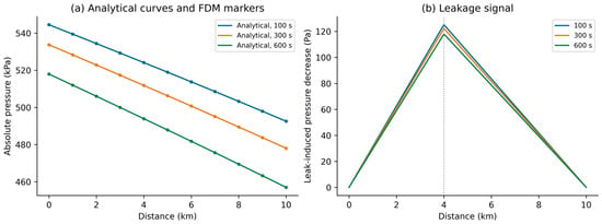
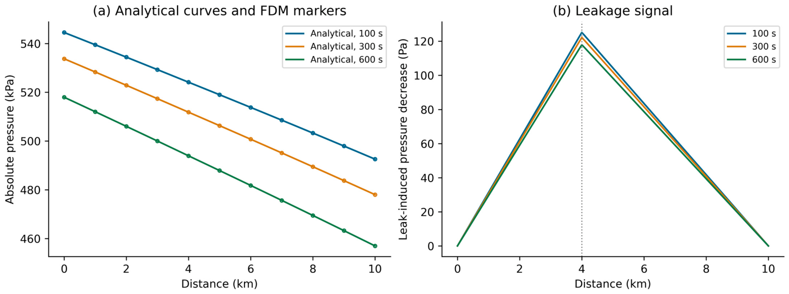
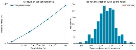
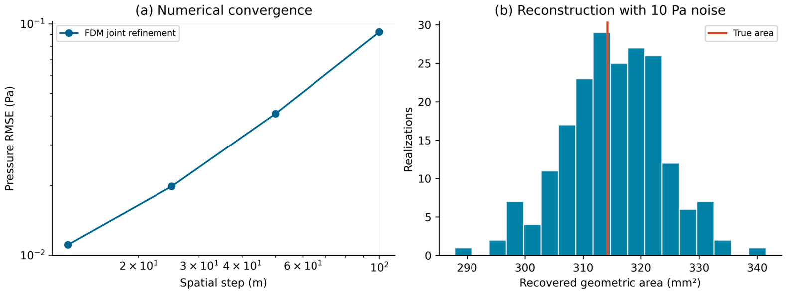
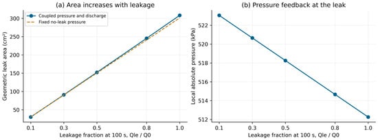

Disclaimer/Publisher’s Note: The statements, opinions and data contained in all publications are solely those of the individual author(s) and contributor(s) and not of MDPI and/or the editor(s). MDPI and/or the editor(s) disclaim responsibility for any injury to people or property resulting from any ideas, methods, instructions or products referred to in the content. |
© 2026 by the authors. Licensee MDPI, Basel, Switzerland. This article is an open access article distributed under the terms and conditions of the Creative Commons Attribution (CC BY) license.