


Abstract
Subdivision schemes are widely used in computer-aided geometric design and computer graphics for generating smooth curves from discrete control polygons. This paper presents a general transformation framework for constructing the corresponding 4-point relaxed quaternary subdivision schemes from 3-point relaxed binary subdivision schemes. The proposed framework requires only the subdivision mask of the binary scheme and is applicable to both parametric and non-parametric subdivision schemes. The resulting quaternary schemes preserve the fundamental properties of their binary counterparts, including continuity, polynomial generation, polynomial reproduction, and shape-preserving characteristics. In many cases, they also possess an enlarged continuity parameter range and increased Hölder regularity. Several examples are presented to demonstrate the applicability of the proposed framework and to illustrate the relationship between the binary subdivision schemes and their corresponding quaternary subdivision schemes. The graphical results show that the transformed quaternary schemes preserve the geometric behavior of their binary counterparts while producing smoother limit curves with fewer subdivision iterations. The proposed framework provides a systematic and efficient approach for establishing the connection between binary and quaternary subdivision schemes and for constructing quaternary schemes directly from existing binary schemes.
1. Introduction
Smooth curve generation from discrete control points is a fundamental problem in computer-aided geometric design (CAGD), computer graphics, industrial design, and digital manufacturing. Subdivision schemes provide an efficient and flexible framework for constructing smooth limit curves through repeated refinement of an initial control polygon. Owing to their simple implementation, local refinement rules, and robust geometric behavior, they have become indispensable tools in applications such as automotive body design, animation, reverse engineering, font design, and geometric modeling [1,2,3,4]. The pioneering Chaikin algorithm [1] laid the foundation for modern subdivision techniques, while subsequent theoretical developments established subdivision schemes as one of the fundamental methodologies in CAGD [2,4,5,6]. Since then, numerous binary, ternary, quaternary, and higher-arity subdivision schemes have been developed to improve smoothness, approximation order, shape-preserving properties, and computational efficiency for a broad range of geometric modeling applications [7,8,9].
Binary subdivision schemes have received considerable attention because of their simple refinement rules, low computational complexity, and ease of implementation. Over the past several decades, extensive research has focused on improving their approximation order, smoothness, shape-preserving behavior, and polynomial reproduction. Dyn et al. [6] established the theoretical foundation for the analysis of uniform binary subdivision schemes by investigating their convergence and smoothness properties. Later, Hao et al. [10] presented the analysis of a 6-point binary approximating subdivision scheme, while Conti and Hormann [7] developed a general framework for polynomial reproduction of univariate subdivision schemes with arbitrary arity. Pana et al. [11] proposed a combined approximating and interpolating subdivision scheme with continuity by incorporating shape parameters, and Siddiqi and Younis [12] introduced a general construction of m-point binary approximating subdivision schemes together with their convergence and smoothness analysis. Romani [13] further modified the classical Lane–Riesenfeld algorithm through a Chaikin-based approach to improve curve approximation. Subsequently, Shi et al. [14] developed 6-point subdivision schemes with cubic precision, whereas Bari et al. [15] demonstrated the applicability of a 7-point binary approximating subdivision scheme for fractal generation. More recently, Zhang [16] investigated several theoretical conjectures related to the classical four-point interpolatory subdivision scheme. Despite these significant developments, binary subdivision schemes often require additional refinement steps to generate highly smooth limit curves, particularly when modeling geometrically complex shapes.
Quaternary subdivision schemes have emerged as an attractive alternative to binary schemes by generating more refined control points during each subdivision step. Consequently, they are capable of producing smooth limit curves with fewer refinement iterations while preserving the geometric characteristics of the initial control polygon. These properties make quaternary subdivision schemes particularly suitable for applications requiring efficient and high-quality curve generation. Mustafa and Khan [17] introduced a 4-point quaternary approximating subdivision scheme, providing one of the earliest contributions to quaternary refinement. Around the same time, Ko [18] proposed a quaternary 4-point approximating subdivision scheme with improved smoothness characteristics. Subsequently, Siddiqi and Younis [19] developed a general algorithm for constructing m-point quaternary approximating subdivision schemes and investigated their convergence and smoothness properties through the corresponding uniform B-spline basis functions. Asghar and Mustafa [8] further established a unified framework for generating families of a-ary subdivision schemes based on Laurent polynomials, providing a systematic approach for constructing higher-arity schemes. More recently, Nawaz et al. [20] proposed a new 7-point quaternary approximating subdivision scheme with enhanced geometric flexibility, whereas Mustafa et al. [21] constructed a family of multiparameter quaternary subdivision schemes to provide additional control over the shape of the limit curves. Yang et al. [22] introduced a family of stationary four-point subdivision schemes with fourth-order accuracy and demonstrated monotonicity- and convexity-preserving properties under suitable conditions. In addition, Amat and Liandrat [23] proposed a nonlinear quaternary approximating subdivision scheme capable of effectively reducing the Gibbs phenomenon while maintaining desirable approximation characteristics. These developments demonstrate the growing interest in quaternary subdivision schemes due to their flexibility, smoothness, and suitability for efficient geometric modeling.
Recent research has focused not only on developing new subdivision schemes but also on establishing systematic relationships between subdivision schemes of different arities. In the non-stationary setting, Daniel and Shunmugaraj [24] developed a non-stationary interpolatory 6-point subdivision scheme with continuity, Siddiqi et al. [25] proposed a non-stationary 6-point binary subdivision scheme derived from hyperbolic basis functions, and Zhang et al. [26] constructed a family of non-stationary combined ternary subdivision schemes reproducing exponential polynomials. In the stationary setting, Hassan et al. [27] introduced a 4-point ternary interpolatory subdivision scheme incorporating a tension parameter for improved shape control. More recently, Hameed et al. [28] proposed a recursive framework for constructing the refinement rules of combined subdivision schemes, and Hameed et al. [29] developed a unified family of subdivision schemes together with algorithms for their analysis and applications to two- and three-dimensional geometric models. Subsequently, Nosheen et al. [30] established a specialized transformation framework relating even-point dual binary subdivision schemes to their corresponding even- and odd-point quaternary subdivision schemes. This idea was further generalized by Hameed et al. [31], who established a transformation framework relating -point dual binary subdivision schemes to -point quaternary subdivision schemes. These studies demonstrate that explicit relationships can be established between binary and quaternary subdivision schemes, allowing the latter to be systematically derived from the former rather than constructed independently. However, these transformation frameworks were developed for dual binary subdivision schemes and rely on their specific refinement structure. They are therefore not directly applicable to primal relaxed binary subdivision schemes, whose vertex and edge refinement rules involve affine combinations of different numbers of control points. Consequently, establishing a transformation framework for relaxed primal subdivision schemes requires a different formulation.
Motivated by this limitation, the present work establishes a general transformation framework relating 3-point relaxed primal binary subdivision schemes to their corresponding 4-point relaxed quaternary subdivision schemes. Unlike the existing transformation frameworks, which are developed for dual binary subdivision schemes, the proposed formulation is specifically designed for the distinct refinement structure of relaxed primal subdivision schemes and establishes explicit relationships between the corresponding binary and quaternary refinement rules. The principal contribution of this work is the establishment of a mathematical bridge between relaxed primal binary and relaxed quaternary subdivision schemes, demonstrating that the corresponding quaternary schemes can be systematically derived from the subdivision masks of their binary counterparts rather than being independently constructed. The proposed framework preserves the essential theoretical properties of the original binary schemes, including continuity, support width, polynomial generation, polynomial reproduction, and shape-preserving behavior. Several illustrative examples are presented to demonstrate the applicability of the proposed framework, while graphical comparisons show that the corresponding quaternary subdivision schemes achieve comparable or smoother limit curves with fewer refinement iterations while preserving the geometric behavior of their binary counterparts.
Although several 4-point quaternary subdivision schemes have been reported in the literature, they have generally been developed independently for specific applications or constructions. In contrast, the present work introduces a general transformation framework that systematically derives the corresponding 4-point relaxed quaternary subdivision schemes directly from existing 3-point relaxed binary subdivision schemes. The proposed framework establishes an explicit mathematical relationship between the two classes of subdivision schemes, requires only the subdivision mask of the binary scheme, and is applicable to both parametric and non-parametric subdivision schemes. Consequently, it provides a unified and systematic approach for constructing quaternary subdivision schemes while preserving the essential theoretical and geometric properties of their binary counterparts.
Applications in Engineering and Industrial Design
The proposed binary-to-quaternary transformation framework is applicable to geometric modeling tasks that require efficient generation of smooth curves from discrete control polygons. Since the transformed quaternary subdivision schemes preserve the essential geometric properties of their binary counterparts while requiring fewer refinement iterations, they reduce the computational effort associated with repeated refinement. Consequently, the proposed framework is suitable for applications in computer-aided geometric design (CAGD), computer-aided design (CAD), industrial product design, animation, reverse engineering, font generation, and digital manufacturing, where efficient curve generation and interactive geometric modeling are essential.
The remainder of the paper is organized as follows. Section 2 presents the essential definitions and preliminary results. Section 3 introduces the proposed transformation framework for constructing the corresponding 4-point relaxed quaternary subdivision schemes from 3-point relaxed binary subdivision schemes. Section 4 presents several illustrative examples and graphical comparisons demonstrating the applicability and effectiveness of the proposed framework. Finally, Section 5 concludes the paper.
2. Fundamental Concepts and Preliminary Results
This section presents the fundamental definitions and preliminary results required for developing the proposed transformation framework and analyzing the results.
Binary and quaternary subdivision schemes recursively generate a sequence of control polygons according to the following refinement rules:
Here, k denotes the subdivision level, r is the refinement index, and . Furthermore,
and
represent the masks of the binary and quaternary subdivision schemes, respectively.
The relaxed binary subdivision schemes considered in this paper are primal subdivision schemes, in which one refinement rule updates the existing vertices of the control polygon, while the other inserts new edge points between consecutive vertices. Unlike the dual binary subdivision schemes considered in the existing transformation frameworks, these schemes possess a distinct primal refinement structure. Specifically, for a 3-point relaxed binary subdivision scheme, the vertex refinement rule is expressed as an affine combination of three consecutive control points, whereas the edge refinement rule is expressed as an affine combination of four consecutive control points. This refinement structure differs fundamentally from that of dual binary subdivision schemes and therefore requires a different transformation framework to establish the relationship with the corresponding relaxed quaternary subdivision schemes.
Remark 1.
The terminology “3-point” and “4-point” follows the standard naming convention in the subdivision literature. Although some refinement rules may involve more than four coefficients due to the relaxation process, a subdivision scheme is classified according to its characteristic stencil rather than the number of coefficients appearing in every refinement rule. Accordingly, the relaxed binary subdivision schemes and their corresponding relaxed quaternary subdivision schemes considered in this paper are referred to as the 3-point and 4-point schemes, respectively.
Definition 1
([9]). A subdivision scheme is said to be -continuous if the limit curve generated by the subdivision process possesses continuous derivatives up to order m. Equivalently, the limit curve belongs to the class , that is, its m-th derivative exists and is continuous.
Definition 2.
Hölder regularity is a measure of the smoothness of the limit function generated by a subdivision scheme. It extends the notion of continuity by providing a quantitative measure of the smoothness of the limit function. A larger Hölder regularity indicates a smoother limit function.
Theorem 1
([4]). Let be the Laurent polynomial of an s-ary subdivision scheme, expressed as
where is a Laurent polynomial and for binary subdivision schemes and for quaternary subdivision schemes. Without loss of generality, let be the nonzero coefficients of , and let be the corresponding matrices defined by
Then, the Hölder regularity of the subdivision scheme is given by
where ξ denotes the joint spectral radius of the matrices . Furthermore,
where denotes the spectral radius of the matrix .
Theorem 2
([12,17]). Let be the Laurent polynomial of an s-ary subdivision scheme, where for binary subdivision schemes and for quaternary subdivision schemes. Then the subdivision scheme generates polynomials of degree k if and only if
where is a Laurent polynomial and
Equivalently, has zeros of order at the zeros of .
Theorem 3
([12,17]). Let be an s-ary subdivision scheme, where for binary subdivision schemes and for quaternary subdivision schemes. Then reproduces polynomials up to degree k with respect to the parametrization
if and only if
where
3. The Main Technique
This section presents the proposed transformation framework for establishing the relationship between the generalized 3-point relaxed binary subdivision scheme and its corresponding 4-point relaxed quaternary subdivision scheme. The framework systematically transforms the binary refinement rules into the corresponding quaternary refinement rules through a sequence of simple substitutions and refinements while preserving the underlying refinement structure.
The generalized -point relaxed binary subdivision scheme is given by
where . Here, and are control points at the -th subdivision step, and are control points at the k-th step. The symmetric subdivision mask is
Setting in (4) yields the 3-point relaxed binary subdivision rules:
For simplicity, the superscript indicating the subdivision level is omitted, and the refinement rules become
The mask of (5) is
3.1. Stepwise Transformation from Binary to Quaternary Subdivision Rules
We begin by systematically deriving the quaternary subdivision rules from the given binary scheme, outlining each transformation step to ensure clarity and reproducibility.
- Transformation Step 1
The transformation begins by replacing with in the binary even-point refinement rule.
- Transformation Step 2
Applying the same substitution to the binary odd-point refinement rule yields the first quaternary odd-point refinement rule.
- Transformation Step 3
Next, the binary even-point rule is evaluated at , generating the second set of quaternary points needed for the scheme.
- Transformation Step 4
Similarly, substituting in the binary odd-point rule produces the final quaternary odd-points.
- Transformation Step 5
With all intermediate points identified, we express them in terms of the original control points, laying the foundation for explicit quaternary formulas.
- Transformation Step 6
Consolidating these expressions allows us to construct explicit formulas for each quaternary subdivision point, fully derived from the binary scheme.
- Transformation Step 7
Finally, reintroducing the subdivision-level superscripts and defining the coefficients , the corresponding 4-point relaxed quaternary subdivision scheme is obtained as
where the coefficients , which represent nonlinear combinations of the coefficients of the 3-point relaxed binary subdivision scheme, are given by
3.2. Alternative Ways to Present the Binary-to-Quaternary Conversion Technique
To improve understanding, the binary-to-quaternary conversion can be represented in multiple formats, including stepwise derivations, block diagrams, tables, and flowcharts, each highlighting different aspects of the procedure.
- Block diagram: Visual representation of the transformation:
- Numbered step-by-step description:
- 1.
- Start with the binary scheme (5).
- 2.
- 3.
- 4.
- Consolidate rules.
- 5.
- Mathematical operator form: , where converts the binary scheme to quaternary.
- Tabular representation: The sequence of substitutions and transformations can be summarized in Table 1, clearly showing the intermediate operations and the resulting quaternary points at each step.
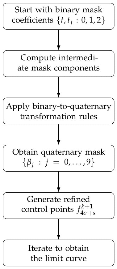
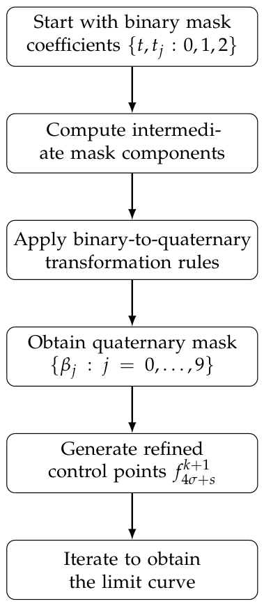
- Flowchart representation: The entire binary-to-quaternary transformation process can be visualized using the flowchart in Figure 1, illustrating the sequential steps from the original binary mask to the final quaternary control points.
Table 1.
Binary-to-quaternary subdivision transformation process.
Figure 1.
Binary-to-quaternary subdivision transformation process.
4. Implementations of the Presented Technique
In this section, we present several examples to illustrate the implementation of the proposed technique. The technique can be applied to both non-parametric and parametric 3-point binary subdivision schemes to investigate their relationship with the corresponding 4-point relaxed quaternary subdivision schemes. The proposed transformation framework always produces a corresponding 4-point relaxed quaternary subdivision scheme. This section also presents graphical representations of the 3-point binary subdivision schemes and their corresponding 4-point relaxed quaternary subdivision schemes at different subdivision levels, as illustrated in the following examples.
4.1. Example
The general Laurent polynomial of the family of subdivision schemes presented by Mustafa and Hameed [32] is given by
where , , and are defined by
Setting in (17) yields the Laurent polynomial of the parametric 3-point relaxed binary subdivision scheme, given by
In the following, we apply the proposed transformation framework to the subdivision scheme associated with the Laurent polynomial (18).
4.1.1. The Binary Subdivision Scheme
The relaxed binary subdivision scheme associated with the Laurent polynomial (18) is
The mask of the binary subdivision scheme (19) is
The subdivision scheme (19) is -continuous when . Using the result of Section 2 on the binary subdivision scheme (19), we obtain a 4-point relaxed quaternary subdivision scheme. We provide a simple illustration of how the 3-point binary subdivision scheme and the 4-point relaxed quaternary subdivision scheme are related. This method uses the mask of the binary subdivision scheme to create the matching 4-point relaxed quaternary subdivision scheme. This method reduced computational effort or fewer refinement iterations.
4.1.2. Main Steps for the Conversion
4.1.3. The Quaternary Subdivision Scheme
The corresponding 4-point relaxed quaternary subdivision scheme is
The Laurent polynomial of the relaxed quaternary subdivision scheme (20) is
The mask of the relaxed quaternary subdivision scheme (20) is
4.1.4. Graphical Comparison
This section presents graphical experiments illustrating the relationship between the 3-point relaxed binary subdivision scheme (19) and the corresponding 4-point relaxed quaternary subdivision scheme (20). The experiments examine the influence of the shape parameter, shape-preserving properties, and real-world data fitting, demonstrating the preserved geometric behavior, smoother approximations, and the wider admissible parameter range of the transformed quaternary subdivision scheme.
Experiment 1.
This experiment illustrates the relationship between the 3-point relaxed binary subdivision scheme (19) and the corresponding 4-point relaxed quaternary subdivision scheme (20) using the closed control polygon with vertices
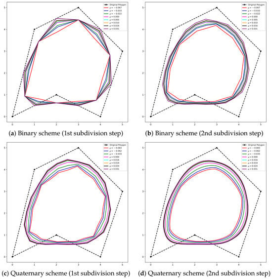
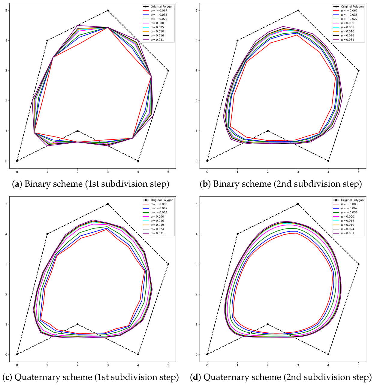
Figure 2 shows the curves generated for different admissible values of the shape parameter . Figure 2a,b present the first and second subdivision steps of the binary subdivision scheme, while Figure 2c,d show the corresponding subdivision steps of the quaternary subdivision scheme. The graphical results demonstrate that both schemes preserve similar geometric behavior under different parameter values. Moreover, the transformed quaternary subdivision scheme admits a wider admissible parameter range and produces smoother approximations after the same number of subdivision steps.
Experiment 2.
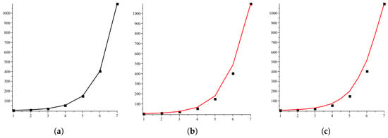
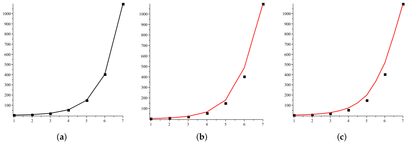
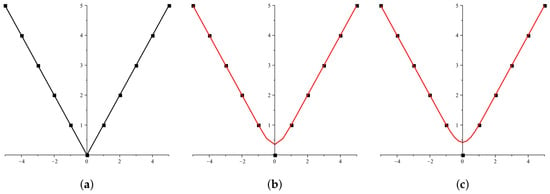
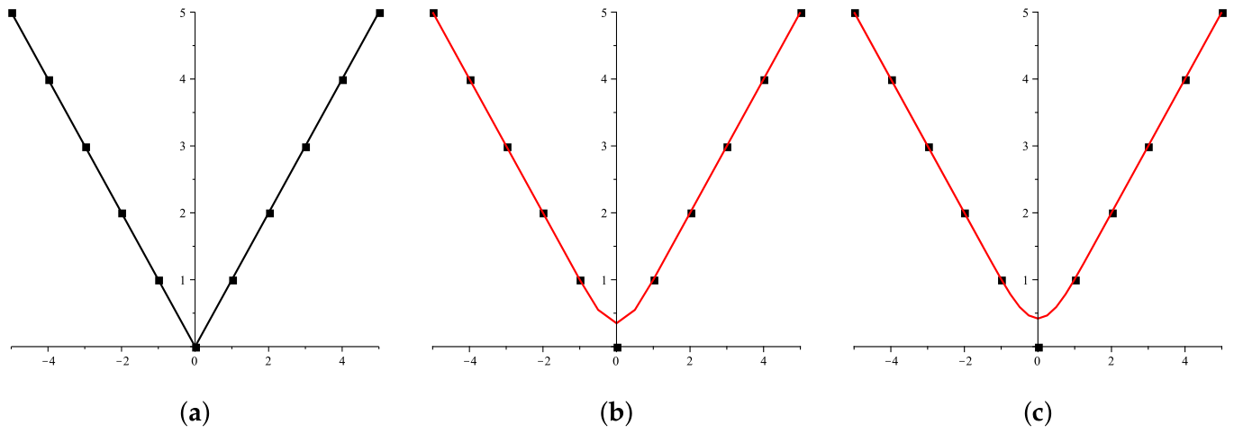
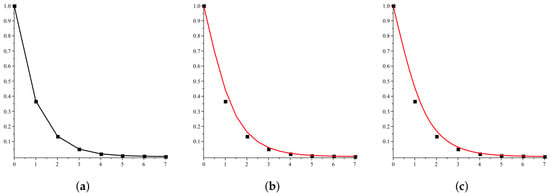
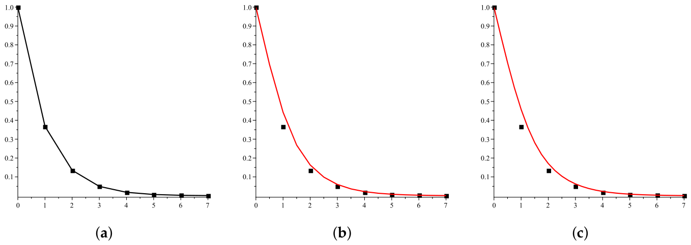
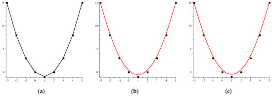
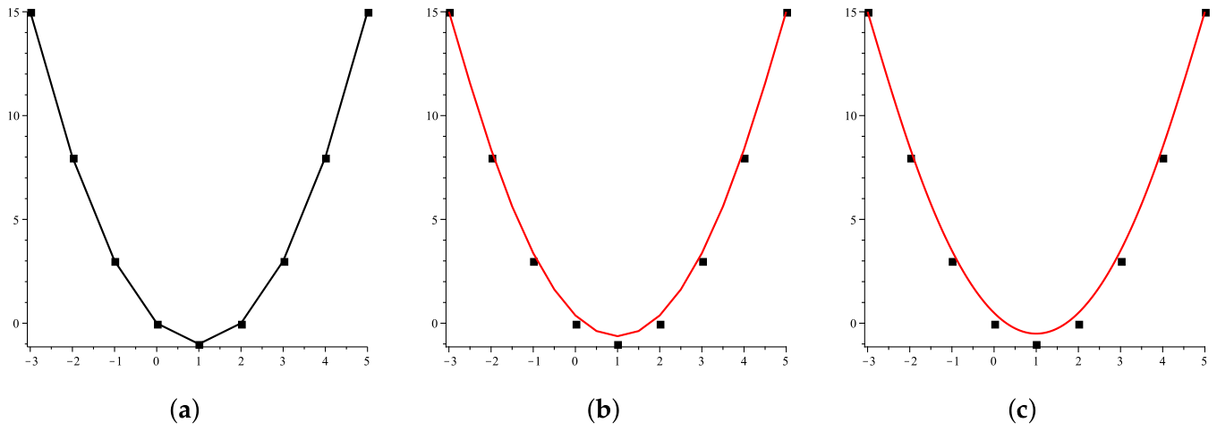
In this experiment, the shape-preserving properties of the 3-point relaxed binary subdivision scheme (19) and the corresponding 4-point relaxed quaternary subdivision scheme (20) are examined. Figure 3 illustrates monotonicity preservation, while Figure 4 illustrates convexity preservation. In each figure, panel (a) shows the initial control polygon, whereas panels (b) and (c) show the curves generated by the binary and corresponding quaternary subdivision schemes, respectively. The graphical results demonstrate that both schemes preserve the monotonicity and convexity of the initial data.
Experiment 3.
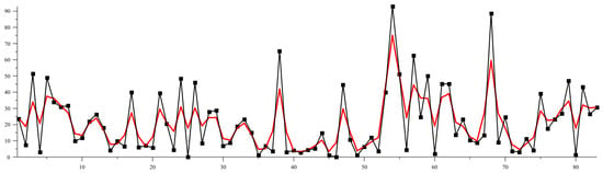
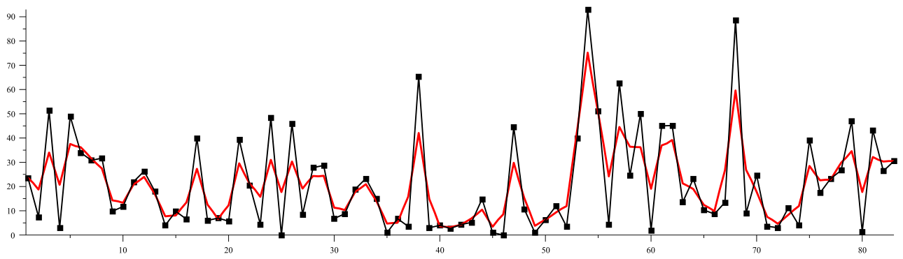
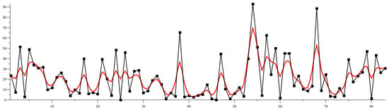
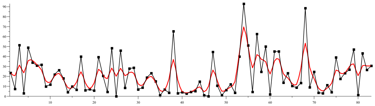
To demonstrate the practical applicability of the proposed framework, a real-world dataset consisting of the daily average ranking positions of a webpage in Google search results is considered. The dataset contains 83 consecutive observations with both gradual and abrupt variations, making it suitable for evaluating the data-fitting capability of subdivision schemes. The corresponding observations are listed in Table 2.
Table 2.
Real-world dataset consisting of daily average webpage ranking positions.
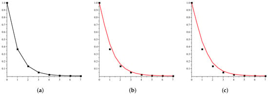
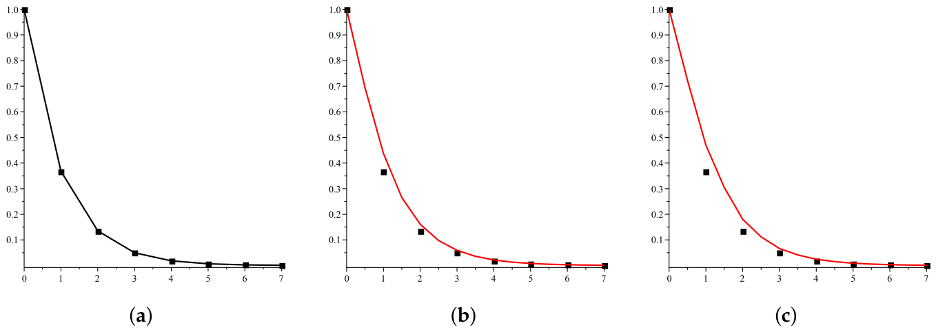
Figure 5 and Figure 6 illustrate the application of the 3-point relaxed binary scheme (19) and its corresponding 4-point relaxed quaternary counterpart (20) to the dataset in Table 2. The observed data are represented by black square markers connected by black line segments to form the initial control polygon. The red curves depict the results obtained after one subdivision step. Both schemes accurately capture the overall trend of the data, while the corresponding quaternary scheme produces a smoother approximation than the binary scheme after one subdivision step.
Figure 5.
Binary subdivision scheme (19). The solid black boxes and black lines represent the initial control points and their corresponding control polyline. The red curve illustrates the result obtained after one subdivision step.
Figure 6.
Corresponding quaternary subdivision scheme (20). The solid black boxes and black lines represent the initial control points and their corresponding control polyline. The red curve illustrates the result obtained after one subdivision step.
4.1.5. Continuity Analysis
Using the Laurent polynomial method, we analyze the continuity of the 3-point binary subdivision scheme (19) and the corresponding 4-point relaxed quaternary subdivision scheme (20). The binary subdivision scheme is -continuous for , whereas the corresponding quaternary subdivision scheme is -continuous for .
Theorem 4.
Proof.
The binary subdivision scheme (19) is -continuous at ; in terms of establishing the continuity of the subdivision scheme, it is sufficient to prove that the difference scheme corresponding to is convergent. Where is the Laurent polynomial of the difference scheme of the scheme corresponding to , which is
To verify the contractiveness of the corresponding difference scheme, we compute
Hence, the binary subdivision scheme (19) is -continuous for
The Laurent polynomial of the corresponding 4-point relaxed quaternary subdivision scheme (20) is
where
The corresponding quaternary subdivision scheme (20) is continuous at ; for establishing the continuity of the subdivision scheme, it is sufficient to prove that the corresponding difference scheme is convergent. Here, represents the Laurent polynomial associated with the difference scheme corresponding to , expressed as follows:
To verify the contractiveness of the subdivision scheme associated with , we examine
Hence, the corresponding 4-point relaxed quaternary subdivision scheme (20) is -continuous for
□
4.1.6. Hölder Regularity Analysis
This subsection analyzes the Hölder regularity of the 3-point binary subdivision scheme and the corresponding 4-point relaxed quaternary subdivision scheme. Hölder regularity provides a quantitative measure of the smoothness of the limit function generated by a subdivision scheme.
Theorem 5.
Proof.
To establish its Hölder regularity, we construct the matrices associated with the Laurent polynomial . From Theorem 1, the matrix entries satisfy
The largest eigenvalues of these matrices are
Moreover,
and
Using Theorem 1, we obtain
Taking , the Hölder regularity of the binary subdivision scheme (19) is
Similarly, the Laurent polynomial of the corresponding 4-point relaxed quaternary subdivision scheme (20) for is
where
From Theorem 1, the coefficients are
with , , and . Hence,
The largest eigenvalues are
and
Furthermore,
Again, using Theorem 1,
Taking , the Hölder regularity of the corresponding 4-point relaxed quaternary subdivision scheme (20) is
Hence, the proof is complete. □
4.1.7. Limit Stencil Analysis
In this subsection, we determine the limit stencils of the 3-point binary subdivision scheme and the corresponding 4-point relaxed quaternary subdivision scheme. The limit stencils characterize the asymptotic refinement behavior of the schemes and provide insight into their approximation properties.
Theorem 6.
Proof.
Consider the 3-point binary subdivision scheme (19). Substituting and into the first and second refinement rules, respectively, and into the second refinement rule yields the subdivision matrix
Hence,
where
are column vectors.
For , the eigenvalues of are
and the corresponding eigenvectors form the columns of the matrix . Thus, the eigendecomposition of is
where
Consequently,
and
Since all eigenvalues of except 1 have modulus less than one,
Therefore,
Hence, the limit stencil of the 3-point binary subdivision scheme (19) is
Now consider the corresponding 4-point relaxed quaternary subdivision scheme (20). Substituting into the third and fourth refinement rules and into the first, second, and third refinement rules yields the subdivision matrix
Hence,
where
are column vectors.
For , the eigenvalues of are
and the corresponding eigenvectors form the columns of the matrix . Thus, the eigendecomposition of is
where
Consequently,
and
Since all eigenvalues of except 1 have a modulus less than one,
Therefore,
Therefore, the limit stencil of the corresponding 4-point relaxed quaternary subdivision scheme (20) is
□
4.1.8. Generation and Reproduction Degrees
In this subsection, we analyze the polynomial generation and reproduction properties of the 3-point binary subdivision scheme (19) and the corresponding 4-point relaxed quaternary subdivision scheme (20).
Theorem 7.
Proof.
The Laurent polynomial of the 3-point binary subdivision scheme (19) can be expressed as
where
Hence, the 3-point binary subdivision scheme (19) generates polynomials of degree 1.
Similarly, the Laurent polynomial of the corresponding 4-point relaxed quaternary subdivision scheme (20) is
where
Therefore, the corresponding 4-point relaxed quaternary subdivision scheme (20) also generates polynomials of degree 1. □
Theorem 8.
Proof.
Using the Laurent polynomial of the 3-point binary subdivision scheme (19) and the conditions in (3), for we obtain
For , we have
Hence, the 3-point binary subdivision scheme (19) reproduces polynomials of degree 1 with respect to the parametrization (3).
Similarly, using the Laurent polynomial of the corresponding 4-point relaxed quaternary subdivision scheme (20) and the conditions in (3), for we obtain
and
For , we obtain
and
4.2. Example
This example illustrates the proposed framework using the parametric binary subdivision scheme introduced by Asghar and Mustafa [8]. They used the Lane–Riesenfield algorithm to show a B-spline symbol for the a-ary subdivision schemes. The standard symbols for their even-ary schemes are defined as
where, and .
According to (31), subdivision schemes with the tension parameter are generated. The values of a and n can be used to readily identify family members.
Substituting and in (31) yields the Laurent polynomial of a parametric 3-point relaxed binary subdivision scheme.
4.2.1. The Binary Subdivision Scheme
The 3-point relaxed binary subdivision scheme associated with the Laurent polynomial (32) depending on parameter is:
This scheme is -continuous for . The mask of the subdivision scheme (33) is
4.2.2. Main Steps for Conversion
Now we can quickly convert the subdivision scheme (33) into its quaternary counterpart by performing just few simple steps as follows:
- By comparing the coefficients of the general form of binary subdivision scheme (5) and the binary subdivision scheme (33), we get the values of the coefficients of the control points, which are:, , , .
- By replacing the values of t, , and into the system of refinement equations given in (16), we obtain the coefficients of the control points as:, , , ,, , ,, , .
- The relaxed 4-point quaternary subdivision scheme is now obtained by inserting the values of in (15).
4.2.3. The Quaternary Subdivision Scheme
4.2.4. The Graphical Comparison
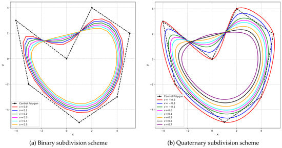
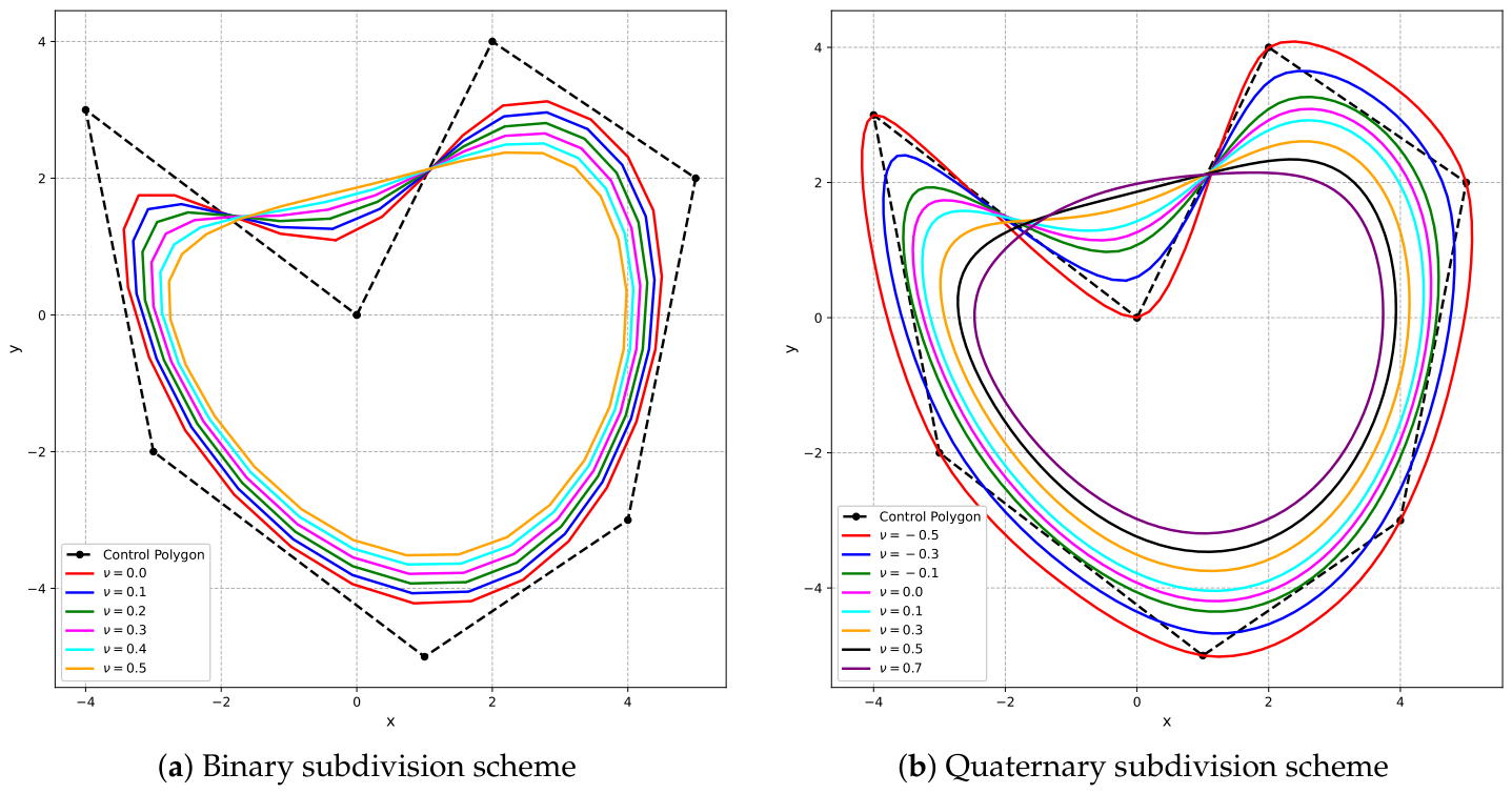
This section presents two graphical experiments illustrating the relationship between the 3-point relaxed binary subdivision scheme (33) and the corresponding 4-point relaxed quaternary subdivision scheme (34) obtained through the proposed transformation. The first experiment investigates the influence of the shape parameter on the generated curves, whereas the second examines the monotonicity- and convexity-preserving properties of the two corresponding subdivision schemes.
Experiment 4.
This experiment illustrates the geometric relationship between the 3-point relaxed binary subdivision scheme (33) and the corresponding 4-point relaxed quaternary subdivision scheme (34) obtained by the proposed transformation. The initial control polygon is defined by the following control points:
Figure 7 presents the curves generated by the binary and the corresponding quaternary subdivision schemes after two subdivision steps for different admissible values of the shape parameter . In both subfigures, the same initial control polygon is used. The resulting curves exhibit similar geometric behavior for the corresponding parameter values, confirming that the transformed quaternary subdivision scheme preserves the geometric characteristics of its binary counterpart. Moreover, because each quaternary subdivision step generates more refined control points than a binary subdivision step, the quaternary scheme produces a visually smoother approximation after the same number of subdivision steps.
Experiment 5.
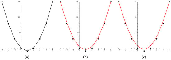
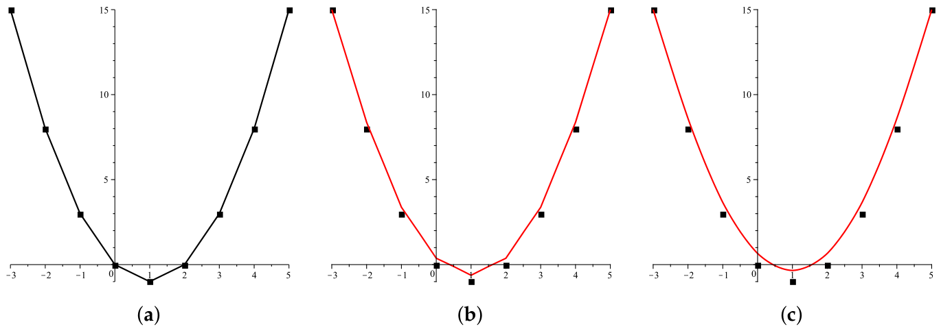
In this experiment, we demonstrated the graphical behavior of monotonicity and convexity preservation of binary subdivision scheme (33) and quaternary subdivision scheme (34). Figure 8 exhibits monotonicity preservation while Figure 9 shows the convexity preservation of the binary (see Figure 8b and Figure 9b) and quaternary (see Figure 8c and Figure 9c) subdivision schemes, respectively.
4.2.5. Theoretical Properties of the Subdivision Schemes
In this section, we analyze the theoretical properties of the 3-point binary and the corresponding 4-point relaxed quaternary subdivision schemes by presenting a series of theorems. These theorems provide insights into the continuity, Hölder regularity, limit stencils, polynomial generation, and polynomial reproduction of the subdivision schemes under specific parameter values. The results presented below provide a theoretical foundation for understanding the behavior of the subdivision schemes.
Theorem 9.
Theorem 10.
Theorem 11.
Remark 3.
The limit stencils of the 3-point binary subdivision scheme (33) and the corresponding 4-point relaxed quaternary subdivision scheme (34) are approximately identical. In both cases, the sum of the stencil coefficients is equal to 1. The central coefficient of the binary subdivision scheme is , whereas that of the corresponding quaternary subdivision scheme is .
Theorem 12.
Theorem 13.
4.2.6. Continuity of Transformed Subdivision Schemes
The proposed transformation framework preserves the continuity of the original binary subdivision scheme while, in many cases, extending the parametric range over which the corresponding quaternary subdivision scheme achieves the same continuity. Consequently, the derived quaternary subdivision schemes exhibit continuity that is at least comparable to, and in some cases greater than, that of their binary counterparts. Furthermore, the higher refinement arity of the quaternary schemes enables the generation of smoother limit curves in fewer subdivision iterations.
Remark 4.
Section 4.1 and Section 4.2 demonstrate that the transformation generally enlarges the parameter intervals for which the corresponding quaternary subdivision schemes attain a prescribed continuity class. This improvement, together with the reduced number of refinement steps required to obtain smooth limit curves, illustrates the effectiveness of the proposed transformation framework.
4.3. Example
This example demonstrates the applicability of the proposed framework to the binary B-spline family which was previously discussed by Hameed et al. [29] in their research. They presented the subdivision rules of the family of -point relaxed approximating schemes, which are actually the binary B-spline schemes. Their presented family of schemes in general form is:
By replacing in (35), we get the B-spline scheme of degree-5, which is the following 3-point relaxed binary subdivision scheme:
The Laurent polynomial of the binary subdivision scheme (36) is
The mask of the binary subdivision scheme (36) is
Now, we follow the same procedure which we have discussed in Section 4.1 and Section 4.2 in detail to get the following 4-point relaxed quaternary subdivision scheme:
The Laurent polynomial of the relaxed quaternary subdivision scheme (37) is
The mask of the relaxed quaternary subdivision scheme (37) is
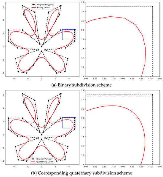
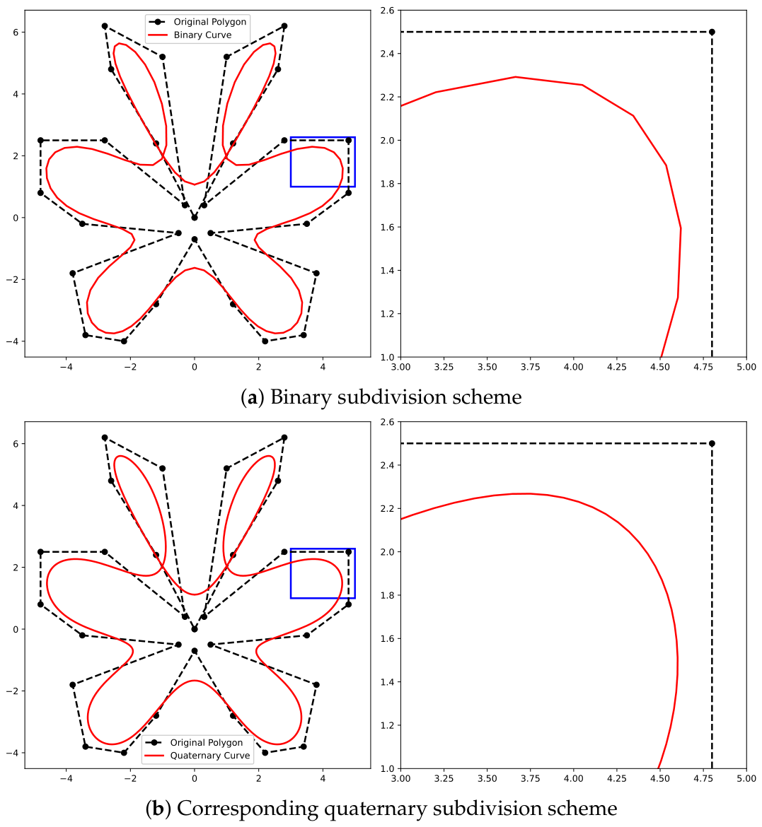
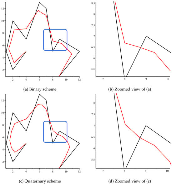
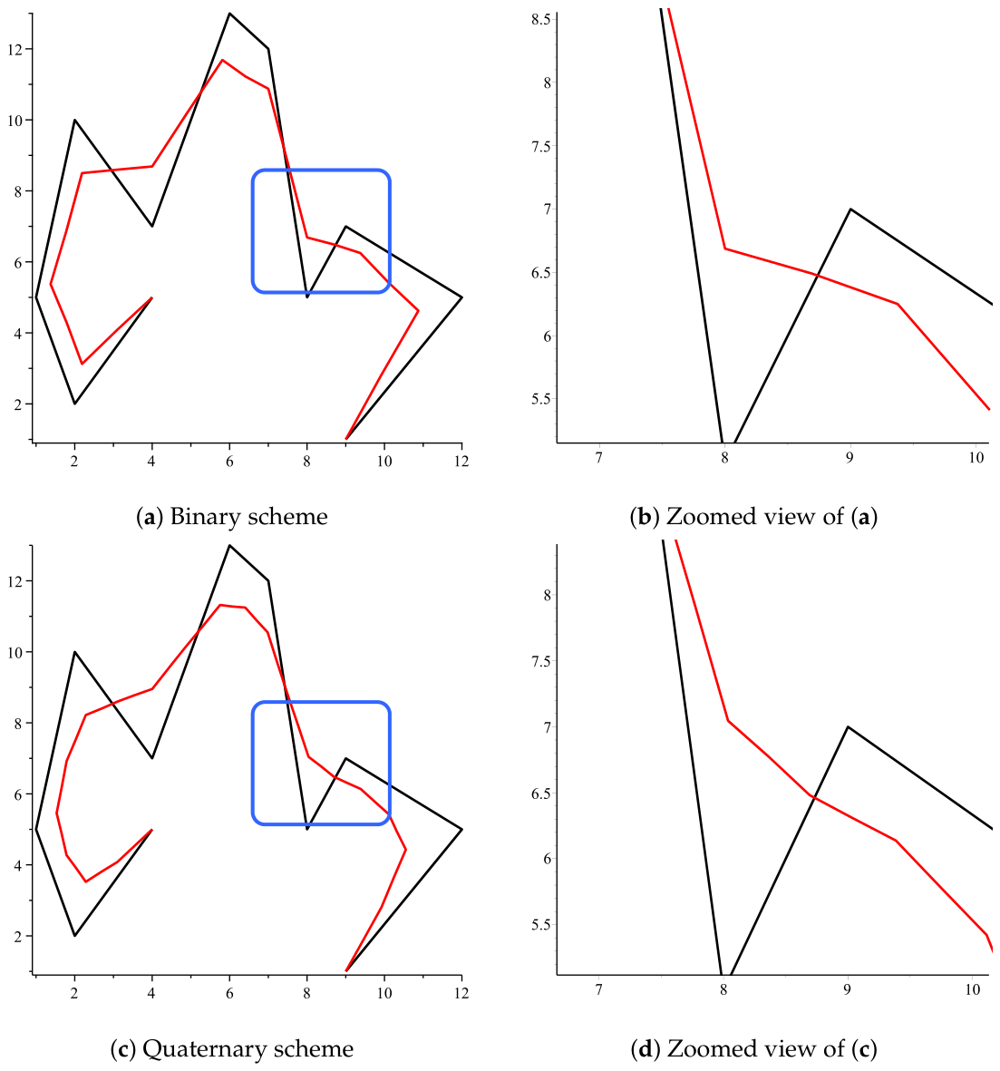
Figure 10 presents a visual comparison of the second subdivision step of the 3-point relaxed binary subdivision scheme (36) and the corresponding 4-point relaxed quaternary subdivision scheme (37). The enlarged views on the right show the regions enclosed by the blue rectangles, illustrating that the transformed quaternary subdivision scheme produces a smoother approximation while preserving the geometric behavior of the corresponding binary subdivision scheme.
Figure 10.
Visual comparison of the second subdivision step and the corresponding enlarged views.
Figure 11 and Figure 12 illustrate that the 3-point binary subdivision scheme (36) and the 4-point quaternary subdivision scheme (37) successfully maintain the monotonicity and convexity of the original data.
Figure 12.
Convexity preservation. (a) Initial control polygon defined by the given control points. (b) Refined curve obtained after one subdivision step using the binary subdivision scheme (35). (c) Refined curve obtained after one subdivision step using the corresponding quaternary subdivision scheme (37).
4.3.1. Visual Justification for Scheme Transformation
Figure 13 compares the first subdivision step of the 3-point relaxed binary subdivision scheme and the corresponding 4-point relaxed quaternary subdivision scheme. Figure 13a,c show the resulting curves, while Figure 13b,d provide enlarged views of the highlighted regions. The graphical comparison shows that the transformed quaternary subdivision scheme preserves the geometric behavior of the corresponding binary subdivision scheme while producing a smoother approximation after the same subdivision step. This visual observation supports the proposed transformation from the binary to the corresponding quaternary subdivision scheme.
Figure 13.
Comparison of the first subdivision step of the 3-point relaxed binary subdivision scheme and the corresponding 4-point relaxed quaternary subdivision scheme. The black polygon represents the initial control polygon, the red curve represents the result of the binary subdivision scheme, and the blue curve represents the result of the corresponding quaternary subdivision scheme. Panels (b,d) show enlarged views of the highlighted regions in panels (a,c), respectively.
4.3.2. Theoretical Properties of the Subdivision Schemes
In this subsection, we analyze the theoretical properties of the 3-point binary and the corresponding 4-point relaxed quaternary subdivision schemes. The following theorems present their continuity, limit stencils, polynomial generation, and polynomial reproduction properties.
Theorem 14.
Theorem 15.
The limit stencil of the 3-point binary subdivision scheme (36) is
while the limit stencil of the 4-point quaternary subdivision scheme (37) is
Remark 5.
The limit stencils of the 3-point binary subdivision scheme (36) and the corresponding 4-point relaxed quaternary subdivision scheme (37) are approximately identical. In both cases, the sum of the stencil coefficients is equal to 1. The central coefficient of the binary subdivision scheme is , whereas that of the corresponding quaternary subdivision scheme is .
Theorem 16.
Theorem 17.
The 3-point binary subdivision scheme (36) reproduces polynomials of degree 5. The corresponding 4-point relaxed quaternary subdivision scheme (37) also reproduces polynomials of degree 5 with respect to the parametrization (3).
The theoretical properties of the binary subdivision scheme and the corresponding relaxed quaternary subdivision scheme are compared in Table 5.
Remark 6.
In Table 3, Table 4 and Table 5, H-Regularity, L-Stencil, P-Reproduction, and P-Generation denote the Hölder regularity, limit stencil, polynomial reproduction, and polynomial generation, respectively. The tables summarize and compare the properties of the binary subdivision schemes and the corresponding relaxed quaternary subdivision schemes presented in Section 4.1, Section 4.2 and Section 4.3.
4.4. Example
A binary subdivision scheme with two shape control parameters was presented by Hameed et al. [28]. Their presented 3-point relaxed subdivision scheme is:
To change the arity of this shape control binary subdivision scheme, we apply the same procedure which we have discussed in the previous examples and get the following 4-point relaxed quaternary subdivision scheme whose parametric coefficients of control points are the nonlinear combination of of the parametric coefficients of the control points of binary subdivision scheme (38):
4.5. Comparison with Existing Quaternary Subdivision Schemes
Although the primary objective of this work is to establish a transformation framework between relaxed binary and corresponding relaxed quaternary subdivision schemes, a comparison with existing 4-point quaternary subdivision schemes is presented to illustrate the theoretical properties and geometric behavior of the derived schemes.
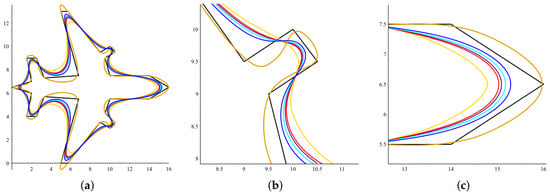
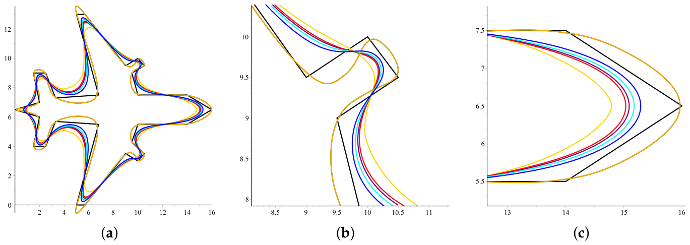
Figure 14 compares the limit curves obtained after three subdivision iterations. The red, niagara purple, and gold curves correspond to the derived quaternary subdivision schemes (20), (34), and (37), respectively, whereas the green, blue, cyan, and orange curves represent the schemes proposed by Mustafa et al. [21], Siddiqi et al. [12], Amat and Liandrat [23], and Ko [18], respectively. The graphical comparison shows that the derived schemes generate smooth limit curves while preserving the geometric characteristics inherited from their corresponding binary subdivision schemes.
Figure 14.
Comparison of the limit curves generated after the third subdivision iteration. (a) Limit curves produced by the derived 4-point quaternary subdivision schemes (20), (34), and (37) together with the existing 4-point quaternary subdivision schemes of Mustafa et al. [21], Siddiqi et al. [12], Amat and Liandrat [23], and Ko [18]. Different colors represent the limit curves generated by the respective subdivision schemes. (b) Enlarged view of the right portion of the limit curves shown in (a). (c) Enlarged view of the bottom-right portion of the limit curves shown in (a).
Table 6 presents a theoretical comparison based on continuity, parameter range, polynomial reproduction, and polynomial generation. The comparison indicates that the derived quaternary subdivision schemes possess theoretical properties comparable to those of the existing schemes, with continuity ranging from to depending on the corresponding binary subdivision scheme.
Table 6.
Comparison of the derived quaternary subdivision schemes with several existing 4-point quaternary subdivision schemes.
Overall, the graphical and theoretical comparisons demonstrate that the proposed transformation framework systematically derives corresponding quaternary subdivision schemes with desirable smoothness and approximation properties while preserving the theoretical characteristics of their binary counterparts.
5. Conclusions
In this work, a theoretical relationship between 3-point relaxed binary and 4-point relaxed quaternary subdivision schemes is established. We have demonstrated that, in some cases, the quaternary schemes are natural extensions of the corresponding binary schemes rather than completely new constructions. Because the proposed transformation framework only uses the subdivision mask of the binary scheme, the procedure is systematic and broadly applicable.
The transformed quaternary schemes preserve the fundamental properties of their corresponding binary schemes, including continuity, polynomial generation, polynomial reproduction, and shape-preserving characteristics. The graphical examples illustrate that the transformed quaternary schemes preserve the geometric behavior of the corresponding binary schemes while producing smoother approximations with fewer subdivision iterations.
In summary, the proposed transformation framework provides a systematic approach for constructing corresponding 4-point relaxed quaternary subdivision schemes directly from existing 3-point relaxed binary subdivision schemes. The resulting quaternary schemes preserve the support size and the fundamental properties of their binary counterparts, providing a unified framework for relating binary and quaternary subdivision schemes.
5.1. Motivation of the Method
An attractive feature of the proposed transformation is that the resulting 4-point relaxed quaternary subdivision schemes retain the same support size as their corresponding 3-point relaxed binary subdivision schemes. Consequently, the increase in arity is achieved without increasing the support size.
5.2. Future Directions
The conversion of subdivision schemes from binary to higher-arity systems remains an active area of research. In this work, a general transformation framework has been presented for constructing corresponding 4-point relaxed quaternary subdivision schemes from 3-point relaxed binary subdivision schemes. An important direction for future research is to investigate whether similar transformation principles can be developed for other classes of binary subdivision schemes and for subdivision schemes of higher-arity.
Another promising direction is the extension of the proposed transformation framework to tensor product subdivision schemes. Since tensor product subdivision schemes play an important role in surface generation for computer graphics and computer-aided geometric design, developing a corresponding binary-to-quaternary transformation framework for surfaces would considerably broaden the applicability of the proposed methodology.
Future work will focus on establishing the theoretical foundations of such transformations, investigating their continuity, polynomial reproduction, approximation, and shape-preserving properties, and validating the resulting schemes through numerical and graphical examples.
Author Contributions
Conceptualization: R.H.; formal analysis: S.S. and R.H.; methodology: R.H. and S.S.; supervision: R.H.; writing—original draft, R.H. and S.S.; analysis: S.N. and J.Y., writing, review and editing: J.Y., M.S.A., R.H. and S.S. All authors agree to be accountable for its content and conclusions. All authors have read and agreed to the published version of the manuscript.
Funding
This research received no external funding.
Data Availability Statement
The original contributions presented in this study are included in the article. Further inquiries can be directed to the corresponding authors.
Conflicts of Interest
The authors declare no conflict of interest.
References
- Chaikin, G.M. An algorithm for high-speed curve generation. Comput. Graph. Image Process. 1974, 3, 346–349. [Google Scholar] [CrossRef] [Scilit]
- Cavaretta, A.S.; Dahmen, W.; Micchelli, C.A. Stationary Subdivision. Mem. Am. Math. Soc. 1991, 93, 1–186. [Google Scholar] [CrossRef] [Scilit]
- Warren, J.; Weimer, H. Subdivision Methods for Geometric Design: A Constructive Approach; Morgan Kaufmann Publishers: San Francisco, CA, USA, 2001. [Google Scholar]
- Dyn, N.; Levin, D. Subdivision schemes in geometric modelling. Acta Numer. 2002, 11, 73–144. [Google Scholar] [CrossRef] [Scilit]
- Dyn, N.; Gregory, J.A.; Levin, D. A 4-point interpolatory subdivision scheme for curve design. Comput. Aided Geom. Des. 1987, 4, 257–268. [Google Scholar] [CrossRef] [Scilit]
- Dyn, N.; Gregory, J.A.; Levin, D. Analysis of uniform binary subdivision schemes for curve design. Constr. Approx. 1991, 7, 127–147. [Google Scholar] [CrossRef] [Scilit]
- Conti, C.; Hormann, K. Polynomial reproduction for univariate subdivision schemes of any arity. J. Approx. Theory 2011, 163, 413–437. [Google Scholar] [CrossRef] [Scilit]
- Asghar, M.; Mustafa, G. Family of a-ary univariate subdivision schemes generated by Laurent polynomial. Math. Probl. Eng. 2018, 2018, 7824279. [Google Scholar] [CrossRef] [Scilit]
- Hussain, S.M.; Rehman, A.U.; Baleanu, D.; Nisar, K.S.; Ghaffar, A.; Abdul Karim, S.A. Generalized 5-point approximating subdivision scheme of varying arity. Mathematics 2020, 8, 474. [Google Scholar] [CrossRef] [Scilit]
- Hao, Y.X.; Wang, R.H.; Li, C.J. Analysis of a 6-point binary subdivision scheme. Appl. Math. Comput. 2011, 218, 3209–3216. [Google Scholar] [CrossRef] [Scilit]
- Pana, J.; Lin, S.; Luo, X. A combined approximating and interpolating subdivision scheme with C2 continuity. Appl. Math. Lett. 2012, 25, 2140–2146. [Google Scholar] [CrossRef] [Scilit]
- Siddiqi, S.S.; Younis, M. Construction of m-point binary approximating subdivision schemes. Appl. Math. Lett. 2013, 26, 337–343. [Google Scholar] [CrossRef] [Scilit]
- Romani, L. A Chaikin-based variant of Lane–Riesenfeld algorithm and its non-tensor product extension. Comput. Aided Geom. Des. 2015, 32, 22–49. [Google Scholar] [CrossRef] [Scilit]
- Shi, J.; Tan, J.; Liu, Z.; Zhang, L. Six-point subdivision schemes with cubic precision. Math. Probl. Eng. 2018, 2018, 2324893. [Google Scholar] [CrossRef] [Scilit]
- Bari, M.; Mustafa, G.; Hussain, A. Fractal generation by 7-point binary approximating subdivision scheme. Int. J. Appl. Phys. Math. 2018, 8, 105–111. [Google Scholar] [CrossRef] [Scilit]
- Zhang, R.J. A few conjectures on a four-point interpolatory subdivision scheme. Comput. Aided Geom. Des. 2020, 82, 101925–101933. [Google Scholar] [CrossRef] [Scilit]
- Mustafa, G.; Khan, F. A New 4-Point C3 Quaternary Approximating Subdivision Scheme. Abstr. Appl. Anal. 2009, 2009, 301967. [Google Scholar] [CrossRef] [Scilit]
- Ko, K.P. A quaternary approximating 4-point subdivision scheme. J. Korean Soc. Ind. Appl. Math. 2009, 13, 307–314. [Google Scholar]
- Siddiqi, S.S.; Younis, M. The m-point quaternary approximating subdivision schemes. Am. J. Comput. Math. 2013, 3, 6–10. [Google Scholar]
- Nawaz, A.; Ghaffar, A.; Khan, F.; Karim, S.A.A. A new 7-point quaternary approximating subdivision scheme. In Intelligent Systems Modeling and Simulation II: Machine Learning, Neural Networks, Efficient Numerical Algorithm and Statistical Methods; Springer International Publishing: Cham, Switzerland, 2022; pp. 545–566. [Google Scholar]
- Mustafa, G.; Asghar, M.; Ali, S.; Qamar, A.; Liu, J.B. The family of multiparameter quaternary subdivision schemes. J. Math. 2021, 2021, 4732464. [Google Scholar] [CrossRef] [Scilit]
- Yang, H.; Kim, K.; Yoon, J. A family of C2 four-point stationary subdivision schemes with fourth-order accuracy and shape-preserving properties. J. Comput. Appl. Math. 2024, 446, 115843. [Google Scholar] [CrossRef] [Scilit]
- Amat, S.; Liandrat, J. On a nonlinear 4-point quaternary approximating subdivision scheme eliminating the Gibbs phenomenon. SeMA J. 2013, 62, 15–25. [Google Scholar] [CrossRef] [Scilit]
- Daniel, S.; Shunmugaraj, P. An interpolating 6-point C2 non-stationary subdivision scheme. J. Comput. Appl. Math. 2009, 230, 164–172. [Google Scholar] [CrossRef] [Scilit]
- Siddiqi, S.S.; us Salam, W.; Rehan, K. A new non-stationary binary 6-point subdivision scheme. Appl. Math. Comput. 2015, 268, 1227–1239. [Google Scholar] [CrossRef] [Scilit]
- Zhang, Z.; Zheng, H.; Pan, L. Construction of a family of non-stationary combined ternary subdivision schemes reproducing exponential polynomials. Open Math. 2021, 19, 909–926. [Google Scholar] [CrossRef] [Scilit]
- Hassan, M.F.; Ivrissimitzis, I.P.; Dodgson, N.A.; Sabin, M.A. An interpolating 4-point C2 ternary stationary subdivision scheme. Comput. Aided Geom. Des. 2002, 19, 1–18. [Google Scholar] [CrossRef] [Scilit]
- Hameed, R.; Mustafa, G.; Deng, J.; Ali, S. Recursive Process for Constructing the Refinement Rules of New Combined Subdivision Schemes and Its Extended Form. J. Math. 2021, 2021, 6639706. [Google Scholar] [CrossRef] [Scilit]
- Hameed, R.; Mustafa, G.; Majeed, R. Variations in 2D and 3D models by a new family of subdivision schemes and algorithms for its analysis. Math. Probl. Eng. 2022, 2022, 3661307. [Google Scholar] [CrossRef] [Scilit]
- Nosheen, S.; Hameed, R.; Younis, J. Establishing a specialized bridge between the even-point binary and the even/odd-point quaternary subdivision approaches. IEEE Access 2024, 12, 78515–78533. [Google Scholar] [CrossRef] [Scilit]
- Hameed, R.; Nosheen, S.; Younis, J. Generalized conversion of (2n + 1)-point binary to 3n + 1-point quaternary subdivision schemes. Sci. Rep. 2025, 15, 6781. [Google Scholar] [CrossRef] [Scilit] [PubMed]
- Mustafa, G.; Hameed, R. Families of univariate and bivariate subdivision schemes originated from quartic B-spline. Adv. Comput. Math. 2017, 43, 1131–1161. [Google Scholar] [CrossRef] [Scilit]

Disclaimer/Publisher’s Note: The statements, opinions and data contained in all publications are solely those of the individual author(s) and contributor(s) and not of MDPI and/or the editor(s). MDPI and/or the editor(s) disclaim responsibility for any injury to people or property resulting from any ideas, methods, instructions or products referred to in the content. |
© 2026 by the authors. Licensee MDPI, Basel, Switzerland. This article is an open access article distributed under the terms and conditions of the Creative Commons Attribution (CC BY) license.