On the Background Driving Lévy Density Associated with the General Tempered Stable Distribution: Theoretical Properties and Financial Applications

Abstract

This paper identifies and characterizes the background driving Lévy process (BDLP) associated with the Generalized Tempered Stable (GTS) distribution, a flexible seven-parameter family of infinitely divisible distributions with applications in physics and quantitative finance. We show that the corresponding BDLP is a finite-variation, infinite-activity Type B Lévy process and derive its explicit background driving characteristic exponent function (BDCEF). The resulting BDLP provides a unified representation that encompasses several important special cases, including the bilateral stable, bilateral Gamma, and Variance Gamma distributions. Building on these results, we develop a simulation framework based on a stationary Ornstein–Uhlenbeck (OU)-type process driven by the GTS BDLP. The mean-reversion speed parameter of the OU process is calibrated using maximum likelihood estimation applied to daily return data from the SPY ETF and Ethereum over the period 2010–2024. The proposed simulation methodology produces realistic daily cumulative return trajectories, and comprehensive numerical error analyses demonstrate the accuracy and efficiency of the resulting discretization scheme. These findings provide both a theoretical extension of Lévy-driven OU models and a practical framework for simulating complex financial return dynamics.

1. Introduction

The modeling of financial asset returns has long challenged the classical assumptions of normality and Geometric Brownian Motion (GBM). Empirical evidence overwhelmingly demonstrates that asset returns exhibit heavy tails, excess kurtosis, asymmetry, and volatility clustering; stylized facts that the normal distribution fails to capture [1,2,3,4,5]. Tempered stable distributions were introduced to overcome the limitations of both stable distribution (which lack finite variance and higher moments) and normal distribution (which underestimates tail risk) [6,7,8,9].

As shown by Rosiński [10], a tempered stable process behaves locally like a stable process, capturing high-intensity small jumps, while its tempered tails ensure the existence of all exponential moments and Gaussian-like behavior over long horizons. These properties make tempered stable models particularly attractive for financial applications, where short-term dynamics are driven by frequent small jumps and long-term returns converge toward diffusive behavior [2,11]. Beyond finance, tempered stable models have also found successful applications in turbulence, plasma physics, solar wind modeling, and other areas of statistical physics [12].

Although the spectral measure provides a complete analytical characterization of tempered stable processes [10,13,14], the Generalized Tempered Stable (GTS) class is one of the most flexible and widely used frameworks. It is constructed by applying exponential tempering (or tilting) to the Lévy measure of an ${\beta }_{\pm }$-stable distribution [15,16]. The resulting six-parameter Lévy measure is given by:

$$M\left(d\xi \right)=\left[{\displaystyle \frac{{\alpha }_{+}}{{\xi }^{1+{\beta }_{+}}}}{e}^{-{\lambda }_{+}\xi }{\mathbf{1}}_{(0,\infty )}\left(\xi \right)+{\displaystyle \frac{{\alpha }_{-}}{{\left|\xi \right|}^{1+{\beta }_{-}}}}{e}^{-{\lambda }_{-}\left|\xi \right|}{\mathbf{1}}_{(-\infty ,0)}\left(\xi \right)\right]d\xi ,$$

(1)

where $\xi \in \mathbb{R}$, $0\le {\beta }_{\pm }\le 1$, ${\alpha }_{\pm }\ge 0$, and ${\lambda }_{\pm }\ge 0$.

This specification nests several well-known Lévy models as special cases. In particular, it includes the KoBoL distribution (${\beta }_{+}={\beta }_{-}$) [12], the truncated Lévy flight (${\lambda }_{+}={\lambda }_{-}$) [16], the bilateral Gamma distribution (${\beta }_{+}={\beta }_{-}=0$) [17,18,19,20], the Variance Gamma distribution (${\alpha }_{+}={\alpha }_{-},{\beta }_{+}={\beta }_{-}=0$) [21,22,23,24,25,26,27], and the Carr–Geman–Madan–Yor (CGMY) class (${\alpha }_{+}={\alpha }_{-},{\beta }_{+}={\beta }_{-}=Y$) [15,28,29].

Although the GTS framework has attracted considerable attention due to its theoretical flexibility and empirical performance [30,31,32], the characterization of the background driving Lévy process (BDLP) underlying the GTS distribution remains relatively unexplored in the literature [33,34]. The BDLP plays a fundamental role in the theory of self-decomposable distributions [35,36,37,38,39,40,41] and in the construction of stationary Ornstein–Uhlenbeck (OU)-type processes, which are widely used in stochastic volatility modeling, time-series analysis, and risk management [42,43,44,45,46,47,48,49].

The present paper fills this gap by investigating the self-decomposable structure of the GTS distribution and deriving explicit analytical expressions for its background driving Lévy density (BDLD) and the corresponding characteristic exponent. Specifically, we show that the GTS distribution is self-decomposable, derive the closed-form BDLD of its associated background driving process, and obtain the characteristic exponent of the corresponding BDLP. We further recover known special cases, including the bilateral stable, bilateral Gamma, and Variance Gamma models. In addition, we develop a simulation framework for OU-type processes driven by the GTS background process using an enhanced Fast Fractional Fourier Transform (FRFT) combined with Newton–Cotes quadrature for numerical inversion [50,51,52]. Finally, we validate the proposed framework using daily return data from the SPY ETF and Ethereum over the period 2010–2024, estimating the mean-reversion speed via maximum likelihood and generating realistic return paths.

The remainder of this paper is structured as follows. Section 2 provides background on Lévy processes, GTS processes, Ornstein–Uhlenbeck dynamics, and self-decomposable distributions. Section 3 establishes the main theoretical results, proving self-decomposability of the GTS distribution and deriving the BDLD and associated characteristic exponents. Section 4 analyzes the BDLP structure and recovers known special cases. Section 5 develops the simulation algorithm for OU-type processes driven by the GTS background driving process and presents numerical experiments for SPY and Ethereum.

2. Preliminaries

2.1. Lévy Framework and Asset Pricing: An Overview

Let $(\mathsf{\Omega },\mathcal{F},{\left\{{\mathcal{F}}_t\right\}}_{t\ge 0},\mathbf{P})$ be a filtered probability space, where $\mathcal{F}={\bigvee }_{t>0}{\mathcal{F}}_t$ and ${\left\{{\mathcal{F}}_t\right\}}_{t\ge 0}$ is a filtration (i.e., ${\mathcal{F}}_{\tau }\subseteq {\mathcal{F}}_t$ for $\tau <t$).

Definition 1.

A stochastic process $L={\left\{L_t\right\}}_{t\ge 0}$ is called a Lévy process if it satisfies the following properties:

(A1) 

$L_0=0$ almost surely.

(A2) 

Independent increments: for any $0<t_1<t_2<\cdots <t_n$, the random variables $L_{t_1}-L_0$, $L_{t_2}-L_{t_1}$, …, $L_{t_n}-L_{t_{n-1}}$ are independent.

(A3) 

Stationary increments: for any $t_1<t_2<+\infty$, the probability distribution of $L_{t_2}-L_{t_1}$ depends only on $t_2-t_1$.

(A4) 

Stochastic continuity: for any $t\ge 0$ and $ϵ>0$, ${\displaystyle \underset{s\to t}{lim}P\left(\right|L_s-L_t| >ϵ)=0}$.

(A5) 

Càdlàg paths: the map $t\mapsto L_t$ is almost surely right-continuous with left limits.

Given a Lévy process $L={\left\{L_t\right\}}_{t\ge 0}$ on the filtered probability space $(\mathsf{\Omega },\mathcal{F},{\left\{{\mathcal{F}}_t\right\}}_{t\ge 0},\mathbf{P})$, we define the asset value process $S={\left\{S_t\right\}}_{t\ge 0}$ by

$$S_t=S_0{e}^{L_t}.$$

Theorem 1

(Lévy–Khintchine representation). Let $L={\left\{L_t\right\}}_{t\ge 0}$ be a Lévy process on $\mathbb{R}$ with characteristic triplet $(\gamma ,{\sigma }^2,M)$. Then, for any $\xi \in \mathbb{R}$ and $t\ge 0$:

$$\begin{array}{cc}\hfill \mathbb{E}\left[e^{i{L}_t\xi }\right]& =e^{t\phi \left(\xi \right)},\hfill \\ \hfill \phi \left(\xi \right):=log\mathbb{E}\left[e^{i{L}_1\xi }\right]& =i\gamma \xi -{\displaystyle \frac{1}{2}}{\sigma }^2{\xi }^2+{\int }_{-\infty }^{+\infty }\left(e^{i\xi y}-1-i\xi y{\mathbf{1}}_{\left|y\right|\le 1}\right)M\left(dy\right),\hfill \end{array}$$

(2)

where $\gamma \in \mathbb{R}$, $\sigma \ge 0$ is the Gaussian coefficient, $\phi \left(\xi \right)$ is the characteristic exponent, and M is the Lévy measure of L satisfying:

$${\int }_{-\infty }^{+\infty }{min(1,|y|}^2)M\left(dy\right)<+\infty .$$

(3)

For a proof of Theorem 1, see [53,54,55].

The Lévy process is completely characterized by its Lévy–Khintchine triplet $(\gamma ,{\sigma }^2,M)$. The triplet suggests that a Lévy process can be decomposed into three independent components: a linear drift, a Brownian motion, and a pure jump Lévy process. When the diffusion term $\sigma =0$, the process reduces to a Lévy jump process; if, in addition, $\gamma =0$, it becomes a pure jump process.

The Lévy–Khintchine representation simplifies when the sample paths of the Lévy process have finite variation on every compact time interval almost surely. A Lévy process has bounded variation [56] if and only if:

$${\sigma }^2=0\mathrm{and}{\int }_{-\infty }^{+\infty }min(1,|x\left|\right)M\left(dx\right)<+\infty .$$

(4)

Under the finite variation assumption, the characteristic exponent $\phi \left(\xi \right)$ in Theorem 1 becomes:

$$\phi \left(\xi \right)=log\mathbb{E}\left[e^{i{L}_1\xi }\right]=i\mathsf{\Gamma }\xi +{\int }_{-\infty }^{+\infty }\left(e^{i\xi y}-1\right)M\left(dy\right),$$

(5)

with:

$${\sigma }^2=0,\mathsf{\Gamma }=\gamma +{\int }_{-1}^{1}xM\left(dx\right).$$

(6)

2.2. Self-Decomposable Laws: Overview

Consider a sequence $(X_k:k=1,2,\dots )$ of independent random variables, but not necessarily identically distributed; and another sequence $(S_n:n=1,2,\dots )$ with $S_n={\sum }_{k=0}^n{X}_k$. We assumed there exist a sequence $(c_n:n=1,2,\dots )$ and a scaling sequence $(b_n:n=1,2,\dots )$ such that ${\displaystyle \frac{S_n+c_n}{b_n}}$ converges in distribution to some random variable X. In other words, the distribution of the random variable X is the limiting distributions of a sequence of normalized sums of independent, but not necessarily identically distributed, random variables. The class of limit laws is known as Lévy class L distributions or class L in the literature [38] and the random variable X is said to belong to Class L. In the classical Central Limit Theorem (CLT), the asymptotically standard normal is of Class L. Likewise, the class of stable laws is of Class L and can be described by four parameters: a location parameter ($\mu$), a scale parameter ($\sigma >0$), a stability index ($0\le \alpha \le 2$) and a skewness parameter ($-1\le \beta \le 1$). The distribution of any random variable in Class L is infinitely divisible [57,58].

In addition, it is shown [54,59] that Class L is also a class of self-decomposable probability distributions. The distribution of a random variable X is self-decomposable if for any constant c ($0<c<1$), there exists an independent random variable $X_c$ such that:

$$\begin{array}{c}\hfill X\stackrel{d}{=}cX+X_c\mathrm{with}X\mathrm{and}{X}_c\mathrm{are}\mathrm{independent}\mathrm{variable}\end{array}$$

(7)

where $\stackrel{d}{=}$ means equality in distribution.

Analytically, a random variable X with a characteristic function $\psi$ is self-decomposable if:

$$\begin{array}{c}\hfill \forall (0<c<1)\exists {\rho }_c\forall (t\in \mathbb{R})\psi \left(t\right)=\psi \left(ct\right){\rho }_c\left(t\right)\end{array}$$

(8)

where ${\rho }_c$ is also a characteristic function.

Class L distributions are also described [60] as distributions of random integrals. Class L is represented as follows:

$$\begin{array}{c}\hfill L=\left\{X={\int }_0^{+\infty }{\mathrm{e}}^{-t}dY\left(s\right),\mathrm{w}\mathrm{i}\mathrm{t}\mathrm{h} Y \mathrm{i}\mathrm{s} \mathrm{a} \mathrm{L}é\mathrm{v}\mathrm{y} \mathrm{P}\mathrm{r}\mathrm{o}\mathrm{c}\mathrm{e}\mathrm{s}\mathrm{s} \mathrm{a}\mathrm{n}\mathrm{d} E\left[log(1+|Y\left(1\right)\left|\right)\right]\le \infty \right\}\end{array}$$

(9)

where the Lévy process ${\left\{Y\left(t\right)\right\}}_{t\ge 0}$ denotes the background driving Lévy process (BDLP) of X.

In terms of characteristic functions, the random integral representation provides an alternative characterization of Class L distributions [60]:

$$X\in \mathrm{Class}L⟺log\psi \left(\xi \right)={\int }_0^{\xi }log\phi \left(u\right){\displaystyle \frac{du}{u}}.$$

(10)

Here, $\psi \left(\xi \right)$ denotes the characteristic function of the random variable X, while $\phi \left(\xi \right)$ denotes the characteristic function of the random variable $Y\left(1\right)$. The function $\phi \left(\xi \right)$ is called the background driving characteristic function (BDCF), and its logarithm, $log\phi \left(\xi \right)$, is referred to as the background driving characteristic exponent function (BDCEF) of X.

The random variable $Y\left(1\right)$ is called the background driving random variable (BDRV) associated with X. Its distribution function,

$$F_{Y\left(1\right)}\left(\xi \right)=P(Y\left(1\right)\le \xi ),\xi \in \mathbb{R},$$

is called the background driving distribution function (BDDF) of X [36].

The relationship between a selfdecomposable variable $\left(X\right)$ and its background driving process can also be featured [60,61] by the triplet in the Lévy–Khintchine Equation (2). Let $\left[A_X,{\sigma }_X^2,M_X\right]$ and $\left[A_Y,{\sigma }_Y^2,N_Y\right]$ be triplets in the Lévy–Khintchine formula for X and Y, respectively. We have:

$$\begin{array}{cc}\hfill M_X\left(A\right)& ={\int }_0^{+\infty }{N}_Y\left({\mathrm{e}}^{t}A\right)dtfor borel subsetsA\subset \mathbb{R}\setminus \left\{0\right\}\hfill \\ \hfill {\sigma }_X^2& ={\displaystyle \frac{1}{2}}{\sigma }_Y^2{A}_X=A_Y+{\int }_{-\infty }^{+\infty }\left({\displaystyle \frac{x}{1+x^2}}-arctan\left(x\right)\right)N_Y\left(dx\right)\hfill \end{array}$$

(11)

The class of self-decomposable probability distributions is very large and includes, among others [36], Stable, Gamma, Log-Gamma, Log-Normal, Chi-Squared (${\chi }^2$), Student-T, Log-Student-T, Fisher–Snedecor and Hyperbolic distributions.

2.3. Ornstein–Uhlenbeck Process: Overview

The Ornstein–Uhlenbeck process is a diffusion process introduced by Ornstein and Uhlenbeck [62] to model the stochastic behavior of the velocity of a particle undergoing Brownian motion. The Ornstein–Uhlenbeck diffusion $X={\left\{X\left(t\right)\right\}}_{t\ge 0}$ is the solution of the Langevin Stochastic Differential Equation (SDE) (12):

$$\begin{array}{c}\hfill d{X}_t=-\lambda X_{t}dt+d{B}_t.\end{array}$$

(12)

where $\lambda >0$ and $B=\{B_t,t\ge 0\}$ is a Brownian motion.

The Ornstein–Uhlenbeck-type process is used in finance to capture important distributional deviations from Gaussianity and to model dependence structures [46,48,63]. The extension of the Ornstein–Uhlenbeck processes is possible by replacing the Brownian motion in (12) by the Lévy process ${\left\{Y_t\right\}}_{t\ge 0}$, called the background driving Lévy process (BDLP) corresponding to the process ${\left\{X_t\right\}}_{t\ge 0}$. The SDE Equation (12) becomes:

$$\begin{array}{c}\hfill d{X}_t=-\lambda X_{t}dt+d{Y}_t\lambda >0.\end{array}$$

(13)

In Equation (13), $dY\left(\lambda t\right)$ is deliberately chosen [46] so that the marginal distribution of X is unchanged, whatever the value of $\lambda$. The solution to the SDE Equation (13) is a stationary process ${\left\{X_t\right\}}_{t\ge 0}$ such that $X_t\stackrel{d}{=}X$. ${\left\{X_t\right\}}_{t\ge 0}$ is a stationary process of the Ornstein–Uhlenbeck type developed in [47,48,64]. ${\left\{X_t\right\}}_{t\ge 0}$ moves up entirely by jumps and then tails off exponentially [46].

Theorem 2.

Let ψ be the characteristic function of a random variable X. If X is self-decomposable, then there exists a stationary stochastic process ${\left\{X\left(t\right)\right\}}_{t>0}$ and a background driving Lévy process (BDLP) ${\left\{L\left(t\right)\right\}}_{t>0}$ independent of $X\left(0\right)$, such that $X\left(t\right)\stackrel{d}{=}X$ and

$$\begin{array}{c}\hfill X\left(t\right)=e^{-\lambda t}X\left(0\right)+{\int }_0^t{e}^{-\lambda (t-s)}d{L}_{\lambda s}\lambda >0.\end{array}$$

(14)

Conversely, if ${\left\{X\left(t\right)\right\}}_{t>0}$ is a stationary stochastic process and ${\left\{L\left(t\right)\right\}}_{t>0}$ is a Lévy process, independent of $X\left(0\right)$, such that ${\left\{X\left(t\right)\right\}}_{t>0}$ and ${\left\{L\left(t\right)\right\}}_{t>0}$ satisfy Equation (13) for all $\lambda >0$, then $X\left(t\right)$ is self-decomposable.

For the theorem-proof, see [47].

2.4. Generalized Tempered Stable (GTS) Distribution: Overview

The GTS distribution is a family of infinitely divisible distributions that generalizes the classical stable laws by introducing exponential tempering into the Lévy measure. This modification preserves the power-law behavior in the central part of the distribution while damping the tails, ensuring the existence of moments and improving the tractability of the model in applications.

Formally, a random variable $Z\sim GTS({\beta }_{+},{\beta }_{-},{\alpha }_{+},{\alpha }_{-},{\lambda }_{+},{\lambda }_{-})$ has a Lévy measure $V\left(dx\right)$ given by Equation (1), where

• ${\beta }_{+},{\beta }_{-}\in (0,1)$ are stability index parameters, controlling the heaviness of the tails on the positive and negative axes, respectively;
• ${\alpha }_{+},{\alpha }_{-}>0$ are scale parameters, determining the overall intensity of jumps;
• ${\lambda }_{+},{\lambda }_{-}>0$ are tempering parameters, governing the exponential decay of large jumps in either direction.

The importance of the Lévy measure is shown by the Lévy–Khintchine representation (Theorem 1), which states that the characteristics of any Lévy process are uniquely defined by a triplet $(a,{\sigma }^2,V)$, consisting of:

• A drift term (a);
• A diffusion or variance coefficient (${\sigma }^2$), which controls the continuous, Gaussian-motion component;
• The Lévy measure (V), which precisely quantifies the frequency and size of the jumps.

As shown in [30,40], GTS distribution is a finite variation process, and generates a type B Lévy process [65], which is a purely non-Gaussian infinite activity Lévy process of finite variation whose sample paths have an infinite number of small jumps and a finite number of large jumps in any finite time interval. In particular, being of bounded variation shows that $Z\sim GTS({\beta }_{+},{\beta }_{-},{\alpha }_{+},{\alpha }_{-},{\lambda }_{+},{\lambda }_{-})$ can be written as the difference of two independent subordinators [66,67]:

$$Z=Z^{+}-Z^{-}\mathrm{with}{Z}^{+}\sim TS({\beta }_{+},{\alpha }_{+},{\lambda }_{+}),Z^{-}\sim TS({\beta }_{-},{\alpha }_{-},{\lambda }_{-}),$$

(15)

where $Z_{+}\sim TS({\beta }_{+},{\alpha }_{+},{\lambda }_{+})$ and $Z_{-}\sim TS({\beta }_{-},{\alpha }_{-},{\lambda }_{-})$ are subordinators.

By adding a drift parameter, we have the following expression:

$$\begin{array}{c}\hfill V=\mu +Z\sim GTS(\mu ,{\beta }_{+},{\beta }_{-},{\alpha }_{+},{\alpha }_{-},{\lambda }_{+},{\lambda }_{-}).\end{array}$$

(16)

Theorem 3.

Consider a variable $V\sim GTS(\mu ,{\beta }_{+},{\beta }_{-},{\alpha }_{+},{\alpha }_{-},{\lambda }_{+},{\lambda }_{-})$; the characteristic exponents can be written as follows:

$$\begin{array}{cc}\hfill \psi \left(\xi \right)& =Log\left(E{e}^{iV\xi }\right)=\mu \xi i+{\psi }^{+}\left(\xi \right)+{\psi }^{-}(-\xi ),\hfill \end{array}$$

(17)

where:

$$\begin{array}{cc}\hfill {\psi }^{+}\left(\xi \right)& =Log\left(E{e}^{i{Z}^{+}\xi }\right)={\alpha }_{+}\mathsf{\Gamma }(-{\beta }_{+})\left({({\lambda }_{+}-i\xi )}^{{\beta }_{+}}-{{\lambda }_{+}}^{{\beta }_{+}}\right),\hfill \\ \hfill {\psi }^{-}\left(\xi \right)& =Log\left(E{e}^{i{Z}^{-}\xi }\right)={\alpha }_{-}\mathsf{\Gamma }(-{\beta }_{-})\left({({\lambda }_{-}-i\xi )}^{{\beta }_{-}}-{{\lambda }_{-}}^{{\beta }_{-}}\right).\hfill \end{array}$$

See [30,68] for Theorem 3 proof.

For illustrative purposes, this study uses the GTS parameter estimates for the SPY ETF and Ethereum reported in [30]. The estimated parameters are summarized in Table 1. Values reported in parentheses correspond to the asymptotic standard errors of the estimators, which were obtained from the inverse of the Hessian matrix evaluated at the maximum likelihood estimates [69,70].

Table 1. GTS parameter estimation for SPY ETF and Ethereum [30].

Parameter	SPY ETF			Ethereum
	Estimate	Std Err	$\mathit{Pr}(\mathit{Z}>|\mathit{z}\left|\right)$	Estimate	Std Err	$\mathit{Pr}(\mathit{Z}>|\mathit{z}\left|\right)$
$\mu$	−0.2606	(0.135)	$5.3\times {10}^{-02}$	−0.4854	(1.008)	$6.3\times {10}^{-01}$
${\beta }_{+}$	0.3408	(0.189)	$7.1\times {10}^{-02}$	0.3904	(0.164)	$1.7\times {10}^{-02}$
${\beta }_{-}$	0.0222	(0.212)	$9.2\times {10}^{-01}$	0.4045	(0.210)	$5.4\times {10}^{-02}$
${\alpha }_{+}$	0.7877	(0.225)	$4.6\times {10}^{-04}$	0.9582	(0.106)	$1.1\times {10}^{-19}$
${\alpha }_{-}$	0.5971	(0.141)	$2.4\times {10}^{-05}$	0.8005	(0.110)	$4.2\times {10}^{-13}$
${\lambda }_{+}$	1.2885	(0.226)	$1.2\times {10}^{-08}$	0.1667	(0.029)	$1.1\times {10}^{-08}$
${\lambda }_{-}$	1.0143	(0.177)	$9.4\times {10}^{-09}$	0.1708	(0.036)	$2.5\times {10}^{-06}$

For all financial assets considered, the maximum likelihood estimates indicate that $\mu$ is negative, while other parameters are positive, as expected in the literature. However, the relatively large standard errors suggest that $\mu$ is not statistically significant at the 5% level. As shown in Table 1, except ${\beta }_{-}$ for SPY ETF, the index of stability parameters (${\beta }_{+}-{\beta }_{-}$), the tempering parameters (${\lambda }_{+}$, ${\lambda }_{-}$) and the scale parameters (${\alpha }_{+}$, ${\alpha }_{-}$) are all statistically significant at the 5% level.

Remark 1.

A comprehensive methodology for fitting the seven-parameter Generalized Tempered Stable (GTS) distribution, together with parameter estimation results, is presented in [30]. The empirical study is based on financial return data from cryptocurrencies and equity markets.

• Data sources: Historical price data for Ethereum (ETH) were obtained from CoinMarketCap. The sample periods span from 7 August 2015 to 4 July 2024 for ETH. Historical prices for the SPY ETF were collected from Yahoo Finance over the period 4 January 2010 to 22 July 2024, with prices adjusted for stock splits and dividend distributions.
• Parameter estimation: The seven GTS parameters were estimated using the Enhanced Fast Fractional Fourier Transform (FRFT) methodology developed in [30,71]. This approach provides an efficient framework for calibrating the flexible class of GTS distributions to financial return data.
• Goodness-of-fit analysis: The adequacy of the fitted models was assessed using the Kolmogorov–Smirnov, Anderson–Darling, and Pearson chi-squared tests. The results indicate that the GTS distribution provides an excellent fit to the data, particularly in capturing heavy tails, skewness, and other departures from normality commonly observed in financial returns.

3. Background Driving Lévy Process (BDLP) of the GTS Distribution

3.1. GTS Background Driving (GTSBD) Lévy Density

Theorem 4.

The Generalized Tempered Stable (GTS) distribution is self-decomposable. Its background driving Lévy process Y is a compound Poisson process with Lévy exponent given by the Lévy density:

$$N\left(dx\right)=\left[{\alpha }_{+}{\displaystyle \frac{{\beta }_{+}+{\lambda }_{+}x}{x^{1+{\beta }_{+}}}}{e}^{-{\lambda }_{+}x}{\mathbf{1}}_{x>0}\right]dx+\left[{\alpha }_{-}{\displaystyle \frac{{\beta }_{-}+{\lambda }_{-}\left|x\right|}{{\left|x\right|}^{1+{\beta }_{-}}}}{e}^{-{\lambda }_{-}\left|x\right|}{\mathbf{1}}_{x<0}\right]dx.$$

(18)

Proof. 

Let $\left[a_{{\psi }^{+}},{\sigma }_{{\psi }^{+}}^2,M_{{\psi }^{+}}\right]$ be the Lévy–Khintchine triplet of the tempered stable distribution $\mathrm{TS}({\beta }_{+},{\alpha }_{+},{\lambda }_{+})$, and let $\left[b_{{\phi }^{+}},s_{{\phi }^{+}}^2,N_{{\phi }^{+}}\right]$ be the Lévy–Khintchine triplet of the associated distribution.

Applying property Equation (11) with $A=(y,+\infty )$ gives:

$$\begin{array}{cc}\hfill M_{{\psi }^{+}}\left((y,+\infty )\right)& ={\int }_y^{+\infty }{\displaystyle \frac{{\alpha }_{+}}{x^{1+{\beta }_{+}}}}{e}^{-{\lambda }_{+}x}dx\hfill \\ \hfill & ={\int }_0^{+\infty }{N}_{{\phi }^{+}}\left((e^{t}y,+\infty )\right)dt={\int }_y^{+\infty }{\displaystyle \frac{N_{{\phi }^{+}}\left((u,+\infty )\right)}{u}}du.\hfill \end{array}$$

(19)

For Equation (19) to hold, we require:

$$N_{{\phi }^{+}}\left((u,+\infty )\right)={\displaystyle \frac{{\alpha }_{+}}{u^{{\beta }_{+}}}}{e}^{-{\lambda }_{+}u}.$$

We carry out differentiating with respect to u yields, and we have the Lévy density:

$$N_{{\phi }^{+}}\left(du\right)=-{\displaystyle \frac{d}{du}}{N}_{{\phi }^{+}}\left((u,+\infty )\right)du={\alpha }_{+}\left({\lambda }_{+}+{\beta }_{+}{u}^{-1}\right)u^{-{\beta }_{+}}{e}^{-{\lambda }_{+}u}du.$$

From Equation (19), the relationship between the Lévy densities $M_{{\psi }^{+}}\left(dy\right)$ and $N_{{\phi }^{+}}\left(dv\right)$ follows:

$$\begin{array}{cc}\hfill M_{{\psi }^{+}}\left(dy\right)& =-{\displaystyle \frac{d{M}_{{\psi }^{+}}\left((y,+\infty )\right)}{dy}}dy={\int }_0^{+\infty }{e}^t{N}_{{\phi }^{+}}\left(e^{t}dy\right)dt\hfill \\ \hfill & ={\int }_0^{+\infty }{\alpha }_{+}\left({\lambda }_{+}+{\beta }_{+}{e}^{-t}{y}^{-1}\right)e^{(1-{\beta }_{+})t}{y}^{-{\beta }_{+}}{e}^{-{\lambda }_{+}y{e}^t}dtdy.\hfill \end{array}$$

Let ${\psi }^{+}\left(\xi \right)$ be the characteristic function of $\mathrm{TS}({\beta }_{+},{\alpha }_{+},{\lambda }_{+})$. Then:

$$log{\psi }^{+}\left(\xi \right)={\int }_0^{+\infty }(e^{iy\xi }-1)M_{{\psi }^{+}}\left(dy\right).$$

Substituting the expression for $M_{{\psi }^{+}}\left(dy\right)$ and changing variables $v=y{e}^t$, $u=e^{-t}$, we obtain:

$$log{\psi }^{+}\left(\xi \right)={\int }_0^1{\int }_0^{+\infty }(e^{i\xi vu}-1){\alpha }_{+}\left({\lambda }_{+}+{\beta }_{+}{v}^{-1}\right)v^{-{\beta }_{+}}{e}^{-{\lambda }_{+}v}dv{\displaystyle \frac{du}{u}}.$$

Thus:

$$log{\psi }^{+}\left(\xi \right)={\int }_0^{1}log{\phi }^{+}\left(\xi u\right){\displaystyle \frac{du}{u}}={\int }_0^{\xi }log{\phi }^{+}\left(x\right){\displaystyle \frac{dx}{x}},x=\xi u.$$

(20)

Here:

$$log{\phi }^{+}\left(x\right)={\int }_0^{+\infty }(e^{ivx}-1)N_{{\phi }^{+}}\left(dv\right),N_{{\phi }^{+}}\left(dx\right)={\alpha }_{+}{\displaystyle \frac{{\beta }_{+}+{\lambda }_{+}x}{x^{1+{\beta }_{+}}}}{e}^{-{\lambda }_{+}x}dx.$$

The same reasoning is applied to the negative side (with parameters ${\beta }_{-},{\alpha }_{-},{\lambda }_{-}$), which gives:

$$log{\psi }^{-}\left(\xi \right)={\int }_0^{\xi }log{\phi }^{-}\left(x\right){\displaystyle \frac{dx}{x}},$$

$$log{\phi }^{-}\left(x\right)={\int }_0^{+\infty }(e^{ivx}-1)N_{{\phi }^{-}}\left(dv\right),N_{{\phi }^{-}}\left(dx\right)={\alpha }_{-}{\displaystyle \frac{{\beta }_{-}+{\lambda }_{-}x}{x^{1+{\beta }_{-}}}}{e}^{-{\lambda }_{-}x}dx.$$

Combining both sides, we define the Lévy density for the GTS distribution:

$$N_{\phi }\left(dx\right)=\left\{\begin{array}{cc}{\alpha }_{+}{\displaystyle \frac{{\beta }_{+}+{\lambda }_{+}x}{x^{1+{\beta }_{+}}}}{e}^{-{\lambda }_{+}x}dx,\hfill & x>0,\hfill \\ {\alpha }_{-}{\displaystyle \frac{{\beta }_{-}+{\lambda }_{-}\left|x\right|}{{\left|x\right|}^{1+{\beta }_{-}}}}{e}^{-{\lambda }_{-}\left|x\right|}dx,\hfill & x<0.\hfill \end{array}\right.$$

Then:

$$log{\phi }^{+}\left(x\right)+log{\phi }^{-}(-x)={\int }_{-\infty }^{+\infty }(e^{ivx}-1)N_{\phi }\left(dv\right).$$

Using Equation (20) and its negative-side counterpart:

$$log{\psi }^{+}\left(\xi \right)+log{\psi }^{-}(-\xi )={\int }_0^{\xi }\left({\int }_{-\infty }^{+\infty }(e^{ivx}-1)N_{\phi }\left(dv\right)\right){\displaystyle \frac{dx}{x}}.$$

(21)

The characteristic exponent of the GTS distribution is therefore:

$$log\psi \left(\xi \right)=log\mathbb{E}{e}^{iX\xi }=i\mu \xi +log{\psi }^{+}\left(\xi \right)+log{\psi }^{-}(-\xi ).$$

From Equation (21):

$$log\psi \left(\xi \right)={\int }_0^{\xi }\left(i\mu x+{\int }_{-\infty }^{+\infty }(e^{ivx}-1)N_{\phi }\left(dv\right)\right){\displaystyle \frac{dx}{x}}={\int }_0^{\xi }log\phi \left(x\right){\displaystyle \frac{dx}{x}},$$

where:

$$log\phi \left(\xi \right)=i\mu x+{\int }_{-\infty }^{+\infty }(e^{ivx}-1)N_{\phi }\left(dv\right).$$

The representation $log\psi \left(\xi \right)={\int }_0^{\xi }log\phi \left(x\right){\displaystyle \frac{dx}{x}}$ is exactly the condition for self-decomposability. Hence, the GTS distribution is self-decomposable.    □

3.2. GTS Background Driving (GTSBD) Characteristic Exponents

Theorem 5 

(Characteristic exponent of the GTS background driving (GTSBD)). The Generalized Tempered Stable (GTS) distribution is self-decomposable. Its background driving Lévy process (BDLP) ${\left\{Y\left(t\right)\right\}}_{t\ge 0}$ has the characteristic exponent:

$$log\phi \left(y\right)=i\mu y+{\alpha }_{+}\mathsf{\Gamma }(1-{\beta }_{+}){\displaystyle \frac{iy}{{({\lambda }_{+}-iy)}^{1-{\beta }_{+}}}}+{\alpha }_{-}\mathsf{\Gamma }(1-{\beta }_{-}){\displaystyle \frac{-iy}{{({\lambda }_{-}+iy)}^{1-{\beta }_{-}}}},$$

(22)

where $\mu \in \mathbb{R}$, ${\alpha }_{\pm }\ge 0$, ${\beta }_{\pm }\in (0,1)$, ${\lambda }_{\pm }>0$, and Γ denotes the Gamma function.

Proof. 

We derive the characteristic exponent by separately computing the contributions from positive and negative jumps. From the Lévy–Khintchine representation (Equation (2)), the positive-jump component satisfies:

$$\begin{array}{cc}\hfill & log{\phi }^{+}\left(x\right)={\int }_0^{+\infty }(e^{ivx}-1){\alpha }_{+}({\lambda }_{+}+{\beta }_{+}{v}^{-1})v^{-{\beta }_{+}}{e}^{-{\lambda }_{+}v}dv\hfill \\ \hfill & ={\displaystyle \sum _{k=1}^{\infty }}{\displaystyle \frac{{\left(ix\right)}^k}{k!}}{\alpha }_{+}\left({\lambda }_{+}{\int }_0^{+\infty }{v}^{k-{\beta }_{+}}{e}^{-{\lambda }_{+}v}dv+{\beta }_{+}{\int }_0^{+\infty }{v}^{-1-{\beta }_{+}}{e}^{-{\lambda }_{+}v}dv\right)\hfill \\ \hfill & ={\displaystyle \sum _{k=1}^{\infty }}{\displaystyle \frac{{\left(ix\right)}^k}{k!}}{\alpha }_{+}\left({\lambda }_{+}{\displaystyle \frac{\mathsf{\Gamma }(k+1-{\beta }_{+})}{{\lambda }_{+}^{k+1-{\beta }_{+}}}}+{\beta }_{+}{\displaystyle \frac{\mathsf{\Gamma }(k-{\beta }_{+})}{{\lambda }_{+}^{k-{\beta }_{+}}}}\right)\hfill \\ \hfill & ={\alpha }_{+}{\lambda }_{+}^{{\beta }_{+}}\mathsf{\Gamma }(1-{\beta }_{+})\left({\displaystyle \sum _{k=1}^{\infty }}{\displaystyle \frac{\mathsf{\Gamma }(k+1-{\beta }_{+})}{\mathsf{\Gamma }(1-{\beta }_{+})k!}}{\left({\displaystyle \frac{ix}{{\lambda }_{+}}}\right)}^k-{\displaystyle \sum _{k=1}^{\infty }}{\displaystyle \frac{\mathsf{\Gamma }(k-{\beta }_{+})}{\mathsf{\Gamma }(-{\beta }_{+})k!}}{\left({\displaystyle \frac{ix}{{\lambda }_{+}}}\right)}^k\right)\hfill \\ \hfill & ={\alpha }_{+}{\lambda }_{+}^{{\beta }_{+}}\mathsf{\Gamma }(1-{\beta }_{+})\left({\displaystyle \sum _{k=1}^{\infty }}\left({\displaystyle \genfrac{}{}{0pt}{}{{\beta }_{+}-1}{k}}\right){\left(-{\displaystyle \frac{ix}{{\lambda }_{+}}}\right)}^k-{\displaystyle \sum _{k=1}^{\infty }}\left({\displaystyle \genfrac{}{}{0pt}{}{{\beta }_{+}}{k}}\right){\left({\displaystyle \frac{ix}{{\lambda }_{+}}}\right)}^k\right).\hfill \end{array}$$

(23)

Using the binomial series expansions,

$${\displaystyle \sum _{k=1}^{\infty }}\left({\displaystyle \genfrac{}{}{0pt}{}{{\beta }_{+}-1}{k}}\right)z^k={(1+z)}^{{\beta }_{+}-1}-1,{\displaystyle \sum _{k=1}^{\infty }}\left({\displaystyle \genfrac{}{}{0pt}{}{{\beta }_{+}}{k}}\right)z^k={(1+z)}^{{\beta }_{+}}-1,$$

with $z=-ix/{\lambda }_{+}$, we obtain:

$$\begin{array}{cc}\hfill log{\phi }^{+}\left(x\right)& ={\alpha }_{+}{\lambda }_{+}^{{\beta }_{+}}\mathsf{\Gamma }(1-{\beta }_{+})\left[{(1-ix/{\lambda }_{+})}^{{\beta }_{+}-1}-1-{(1-ix/{\lambda }_{+})}^{{\beta }_{+}}+1\right]\hfill \\ \hfill & ={\alpha }_{+}{\lambda }_{+}^{{\beta }_{+}}\mathsf{\Gamma }(1-{\beta }_{+})\left[{(1-ix/{\lambda }_{+})}^{{\beta }_{+}-1}-{(1-ix/{\lambda }_{+})}^{{\beta }_{+}}\right]\hfill \\ \hfill & ={\alpha }_{+}\mathsf{\Gamma }(1-{\beta }_{+})\left[{\lambda }_{+}{({\lambda }_{+}-ix)}^{{\beta }_{+}-1}-{({\lambda }_{+}-ix)}^{{\beta }_{+}}\right]\hfill \\ \hfill & ={\alpha }_{+}\mathsf{\Gamma }(1-{\beta }_{+}){\displaystyle \frac{ix}{{({\lambda }_{+}-ix)}^{1-{\beta }_{+}}}}.\hfill \end{array}$$

A similar computation for the negative jumps yields:

$$\begin{array}{cc}\hfill log{\phi }^{-}(x)& ={\int }_{-\infty }^0(e^{ivx}-1){\alpha }_{-}({\lambda }_{-}+{\beta }_{-}{\left|v\right|}^{-1}{\left)\right|v|}^{-{\beta }_{-}}{e}^{-{\lambda }_{-}\left|v\right|}dv\hfill \\ \hfill & ={\int }_0^{+\infty }(e^{-ivx}-1){\alpha }_{-}({\lambda }_{-}+{\beta }_{-}{v}^{-1})v^{-{\beta }_{-}}{e}^{-{\lambda }_{-}v}dv\hfill \\ \hfill & ={\alpha }_{-}\mathsf{\Gamma }(1-{\beta }_{-}){\displaystyle \frac{-ix}{{({\lambda }_{-}+ix)}^{1-{\beta }_{-}}}}.\hfill \end{array}$$

The total characteristic exponent is the sum of the drift and the two jump components:

$$log\phi \left(x\right)=i\mu x+log{\phi }^{+}\left(x\right)+log{\phi }^{-}\left(x\right).$$

(24)

Substituting the expressions above gives:

$$log\phi \left(x\right)=i\mu x+{\alpha }_{+}\mathsf{\Gamma }(1-{\beta }_{+}){\displaystyle \frac{ix}{{({\lambda }_{+}-ix)}^{1-{\beta }_{+}}}}+{\alpha }_{-}\mathsf{\Gamma }(1-{\beta }_{-}){\displaystyle \frac{-ix}{{({\lambda }_{-}+ix)}^{1-{\beta }_{-}}}},$$

which is exactly Equation (22). This completes the proof.    □

4. GTS Background Driving (GTSBD) Distribution: Theoretical Properties

As shown in Theorem 4, the background driving Lévy density (BDLD) associated with the Generalized Tempered Stable (GTS) distribution differs from the GTS Lévy measure Equation (1). Specifically, the BDLD is expressed as the product of a tempering (or tilting) function $q\left(y\right)$ and a rational function $Q\left(y\right)$, defined as follows:

$$\begin{array}{cc}\hfill q\left(y\right)& =exp(-{\lambda }_{+}y){\mathbf{1}}_{(0,\infty )}\left(y\right)+exp(-{\lambda }_{-}\left|y\right|){\mathbf{1}}_{(-\infty ,0)}\left(y\right),\hfill \end{array}$$

(25)

$$\begin{array}{cc}\hfill Q\left(y\right)& ={\alpha }_{+}{\displaystyle \frac{{\beta }_{+}+{\lambda }_{+}y}{y^{1+{\beta }_{+}}}}{\mathbf{1}}_{(0,\infty )}\left(y\right)+{\alpha }_{-}{\displaystyle \frac{{\beta }_{-}+{\lambda }_{-}\left|y\right|}{{\left|y\right|}^{1+{\beta }_{-}}}}{\mathbf{1}}_{(-\infty ,0)}\left(y\right).\hfill \end{array}$$

(26)

Consider a background driving random variable (BDRV) Y associated with the GTS distribution. Then, Y follows a background driving distribution, denoted as GTSBD $({\beta }_{+},{\beta }_{-},{\alpha }_{+},{\alpha }_{-},{\lambda }_{+},{\lambda }_{-})$, defined by the Lévy measure $N\left(dy\right)$, given by:

$$N\left(dy\right)=\left[{\alpha }_{+}{\displaystyle \frac{{\beta }_{+}+{\lambda }_{+}y}{y^{1+{\beta }_{+}}}}{e}^{-{\lambda }_{+}y}{\mathbf{1}}_{y>0}\right]dy+\left[{\alpha }_{-}{\displaystyle \frac{{\beta }_{-}+{\lambda }_{-}\left|y\right|}{{\left|y\right|}^{1+{\beta }_{-}}}}{e}^{-{\lambda }_{-}\left|y\right|}{\mathbf{1}}_{y<0}\right]dy.$$

(27)

The activity process of the GTSBD distribution can be studied via the integral of the Lévy measure in Equation (27):

$${\int }_{-\infty }^{+\infty }N\left(dy\right)=+\infty \mathrm{for}{\beta }_{+},{\beta }_{-}\in (0,1).$$

(28)

As shown in Equation (28), when ${\beta }_{+},{\beta }_{-}\in (0,1)$, the Lévy measure $N\left(dy\right)$ is not integrable [68]; it diverges as $y\to 0$ due to an accumulation of very small jumps [72]. Consequently, the GTSBD distribution exhibits infinite activity, meaning that its sample paths have an infinite number of very small jumps within any finite time interval.

The variation in the background driving process can be assessed using the following integral condition [66]:

$${\int }_{-\infty }^{+\infty }min(1,|x\left|\right)N\left(dx\right)<+\infty \mathrm{for}{\beta }_{+},{\beta }_{-}\in (0,1).$$

(29)

Condition Equation (29) implies that the GTSBD distribution is a finite-variation process (see refs. [40,68] for further developments). It generates a Type B Lévy process [56,65]: a purely non-Gaussian, infinite-activity Lévy process of finite variation whose sample paths contain infinitely many small jumps but only finitely many large jumps in any finite time interval.

Because the process has bounded variation, $Y\sim \mathrm{GTSBD}({\beta }_{+},{\beta }_{-},{\alpha }_{+},{\alpha }_{-},{\lambda }_{+},{\lambda }_{-})$ can be written as the difference of two independent subordinators [66,67]:

$$Y=Y^{+}-Y^{-},$$

(30)

Adding a drift parameter $\mu$ yields the GTSBD distribution:

$$\mu +Y\sim \mathrm{GTSBD}(\mu ,{\beta }_{+},{\beta }_{-},{\alpha }_{+},{\alpha }_{-},{\lambda }_{+},{\lambda }_{-}).$$

(31)

Properties of Background Driving Lévy Density (BDLD)

The GTSBD distribution introduced in Equation (27) enjoys a remarkable structural property: its BDLD interpolates between several well-known distribution families as its parameters approach boundary values. These connections, summarized in Theorem 6 below, highlight the flexibility and unifying nature of the GTSBD framework within the class of tempered stable processes.

Theorem 6.

Let

$$\begin{array}{c}\hfill Y\sim GTSBD(\mu ,{\beta }_{+},{\beta }_{-},{\alpha }_{+},{\alpha }_{-},{\lambda }_{+},{\lambda }_{-}).\end{array}$$

(32)

Then, the following results hold:

1. 

Suppose that $({\lambda }_{-},{\lambda }_{+})\to (0,0)$; then, the background driving Lévy density (BDLD) associated with the bilateral stable distribution with characteristic exponent

$$\begin{array}{c}\hfill log\left(\psi \left(x\right)\right)=i\mu \xi +{\alpha }_{+}\mathsf{\Gamma }(-{\beta }_{+}){(-ix)}^{{\beta }_{+}}+{\alpha }_{-}\mathsf{\Gamma }(-{\beta }_{-}){\left(ix\right)}^{{\beta }_{-}}\end{array}$$

is again a bilateral stable distribution with characteristic exponent

$$\begin{array}{c}\hfill log\left(\phi \left(x\right)\right)=i\mu x-{\alpha }_{+}\mathsf{\Gamma }(1-{\beta }_{+}){(-ix)}^{{\beta }_{+}}-{\alpha }_{-}\mathsf{\Gamma }(1-{\beta }_{-}){\left(ix\right)}^{{\beta }_{-}}.\end{array}$$

(33)

2. 

Suppose that $({\beta }_{-},{\beta }_{+})\to (0,0)$; then, the background driving Lévy density (BDLD) associated with the Bilateral Gamma (BG) distribution, whose characteristic exponent is given by

$$\begin{array}{c}\hfill log\left(\psi \left(x\right)\right)=i\mu x+{\alpha }_{+}log\left(1-{\displaystyle \frac{ix}{{\lambda }_{+}}}\right)-{\alpha }_{-}log\left(1+{\displaystyle \frac{ix}{{\lambda }_{-}}}\right),\end{array}$$

has characteristic exponent

$$\begin{array}{c}\hfill log\left(\phi \left(x\right)\right)=i\mu x+{\alpha }_{+}{\displaystyle \frac{ix}{{\lambda }_{+}-ix}}-{\alpha }_{-}{\displaystyle \frac{ix}{{\lambda }_{-}+ix}}.\end{array}$$

(34)

3. 

In addition to the condition $({\beta }_{-},{\beta }_{+})\to (0,0)$, assume that ${\alpha }_{-}={\alpha }_{+}=\alpha$; then, the background driving Lévy density (BDLD) associated with the Variance Gamma (VG) distribution, whose characteristic exponent is:

$$\begin{array}{c}\hfill log\left(\psi \left(x\right)\right)=i\mu x-\alpha log\left(1-{\displaystyle \frac{{\lambda }_{-}-{\lambda }_{+}}{{\lambda }_{+}{\lambda }_{-}}}ix+{\displaystyle \frac{x^2}{{\lambda }_{+}{\lambda }_{-}}}\right),\end{array}$$

and has the characteristic exponent

$$\begin{array}{c}\hfill log\left(\phi \left(x\right)\right)=i\mu x-2\alpha +\alpha \left({\displaystyle \frac{{\lambda }_{+}}{{\lambda }_{+}-ix}}+{\displaystyle \frac{{\lambda }_{-}}{{\lambda }_{-}+ix}}\right).\end{array}$$

(35)

Proof. 

We examine the limiting behavior of the characteristic exponent of the GTS background driving (GTSBD) distribution, $log\phi \left(x\right)$ in Equation (22), under three parametric regimes.

• Case 1: ${\lambda }_{\pm }\to 0$. Taking the limit gives:

  $$\underset{{\lambda }_{\pm }\to 0}{lim}log\phi \left(x\right)=i\mu x-{\alpha }_{+}\mathsf{\Gamma }(1-{\beta }_{+}){(-ix)}^{{\beta }_{+}}-{\alpha }_{-}\mathsf{\Gamma }(1-{\beta }_{-}){\left(ix\right)}^{{\beta }_{-}}.$$
  This is precisely the characteristic exponent of the BDLD associated with the bilateral stable distribution, as stated in part 1 of the theorem.
• Case 2: ${\beta }_{\pm }\to 0$. In this setting, we obtain:

  $$\underset{{\beta }_{\pm }\to 0}{lim}log\phi \left(x\right)=i\mu x+{\alpha }_{+}{\displaystyle \frac{ix}{{\lambda }_{+}-ix}}+{\alpha }_{-}{\displaystyle \frac{-ix}{{\lambda }_{-}+ix}}.$$
  This characterizes the BDLD associated with the Bilateral Gamma distribution.
• Case 3: ${\beta }_{\pm }\to 0$ and ${\alpha }_{-}={\alpha }_{+}=\alpha$. Under these additional symmetry assumptions, the limit reduces to:

  $$\underset{{\beta }_{\pm }\to 0}{lim}log\phi \left(x\right)=i\mu x+\alpha \left({\displaystyle \frac{ix}{{\lambda }_{+}-ix}}+{\displaystyle \frac{-ix}{{\lambda }_{-}+ix}}\right),$$

  which is the characteristic exponent of the BDLD corresponding to the Variance Gamma (VG) distribution.

Therefore, the background driving characteristic exponent function (BDCEF) associated to the GTS distribution encompasses the Bilateral Stable, Bilateral Gamma and Variance Gamma distributions as limiting cases, illustrating the unifying nature of the GTS BDLD framework.    □

Remark 2.

Part 1 of Theorem 6 shows that the background driving distribution associated with a bilateral stable distribution remains within the class of bilateral stable distributions. Specifically, it preserves the stability index parameters ${\beta }_{\pm }$, with only the scale parameters being modified. Consequently, the background driving Lévy process (BDLP) corresponding to a bilateral stable marginal distribution is itself bilateral stable. This structural invariance is especially useful for simulation purposes, as it implies that Ornstein–Uhlenbeck (OU) processes driven by bilateral stable Lévy processes, as well as OU processes with bilateral stable stationary marginals, admit exact simulation schemes (see [73,74]).

Theorem 7

(GTSBD Cumulants ${\kappa }_k$). Consider a variable $Y\sim GTS(\mu ,{\beta }_{+},{\beta }_{-},{\alpha }_{+},{\alpha }_{-},{\lambda }_{+},{\lambda }_{-})$. The cumulants ${\kappa }_k$ of the GTS distribution are defined as follows:

$$\begin{array}{cc}\hfill {\kappa }_1& =\mu +{\alpha }_{+}{\displaystyle \frac{\mathsf{\Gamma }(1-{\beta }_{+})}{{\lambda }_{+}^{1-{\beta }_{+}}}}-{\alpha }_{-}{\displaystyle \frac{\mathsf{\Gamma }(1-{\beta }_{-})}{{\lambda }_{-}^{1-{\beta }_{-}}}}{\kappa }_2=2\left({\alpha }_{+}{\displaystyle \frac{\mathsf{\Gamma }(2-{\beta }_{+})}{{\lambda }_{+}^{2-{\beta }_{+}}}}+{\alpha }_{-}{\displaystyle \frac{\mathsf{\Gamma }(2-{\beta }_{-})}{{\lambda }_{-}^{2-{\beta }_{-}}}}\right)\hfill \\ \hfill {\kappa }_k& =k\left({\alpha }_{+}{\displaystyle \frac{\mathsf{\Gamma }(k-{\beta }_{+})}{{\lambda }_{+}^{k-{\beta }_{+}}}}+{\alpha }_{-}{\displaystyle \frac{\mathsf{\Gamma }(k-{\beta }_{-})}{{\lambda }_{-}^{k-{\beta }_{-}}}}{(-1)}^k\right)\forall k\in \mathbb{N}\setminus \{0,1\}.\hfill \end{array}$$

(36)

Proof. 

We reconsider the characteristic exponent $\phi \left(\xi \right)$ in Equation (22). From Equation (23), we have: 

$$\begin{array}{cc}\hfill log\left({\phi }^{+}\left(x\right)\right)& ={\int }_0^{+\infty }(e^{ivx}-1){\alpha }_{+}({\lambda }_{+}+{\beta }_{+}{v}^{-1})v^{-{\beta }_{+}}{e}^{-{\lambda }_{+}v}dv\hfill \\ \hfill & ={\displaystyle \sum _{k=1}^{\infty }}{\displaystyle \frac{{\left(ix\right)}^k}{k!}}{\alpha }_{+}\left({\lambda }_{+}{\int }_0^{+\infty }{v}^{k-{\beta }_{+}}{e}^{-{\lambda }_{+}v}dv+{\beta }_{+}{\int }_0^{+\infty }{v}^{-1-{\beta }_{+}}{e}^{-{\lambda }_{+}v}dv\right)\hfill \\ \hfill & ={\displaystyle \sum _{k=1}^{\infty }}{\displaystyle \frac{{\left(ix\right)}^k}{k!}}{\alpha }_{+}\left({\lambda }_{+}{\displaystyle \frac{\mathsf{\Gamma }(k+1-{\beta }_{+})}{{\lambda }_{+}^{k+1-{\beta }_{+}}}}+{\beta }_{+}{\displaystyle \frac{\mathsf{\Gamma }(k-{\beta }_{+})}{{\lambda }_{+}^{k-{\beta }_{+}}}}\right)\hfill \\ \hfill & ={\alpha }_{+}{\displaystyle \sum _{k=1}^{\infty }}{\displaystyle \frac{k\mathsf{\Gamma }(k-{\beta }_{+})}{{\lambda }_{+}^{k-{\beta }_{+}}}}{\displaystyle \frac{{\left(ix\right)}^k}{k!}}.\hfill \end{array}$$

(37)

Similarly, we have:

$$\begin{array}{c}\hfill log\left({\phi }^{-}\left(x\right)\right)={\alpha }_{-}{\displaystyle \sum _{k=1}^{\infty }}{\displaystyle \frac{k\mathsf{\Gamma }(k-{\beta }_{-})}{{\lambda }_{-}^{k-{\beta }_{-}}}}{\displaystyle \frac{{(-ix)}^k}{k!}}.\end{array}$$

We have:  

$$\begin{array}{c}\hfill log\left(\phi \left(x\right)\right)=\mu xi+log\left({\phi }^{+}\left(x\right)\right)+log\left({\phi }^{-}(-x)\right)\end{array}$$

(38)

$$\begin{array}{cc}\hfill log\left(\phi \left(x\right)\right)& =i\mu x+log\left({\phi }^{+}\left(x\right)\right)+log\left({\phi }^{-}(-x)\right)\hfill \\ \hfill & =i\mu x+{\displaystyle \sum _{k=1}^{\infty }}\left[{\alpha }_{+}{\displaystyle \frac{\mathsf{\Gamma }(k-{\beta }_{+})}{{\lambda }_{+}^{k-{\beta }_{+}}}}+{\alpha }_{-}{\displaystyle \frac{\mathsf{\Gamma }(k-{\beta }_{-})}{{\lambda }_{-}^{k-{\beta }_{-}}}}{(-1)}^k\right]{\displaystyle \frac{{\left(ix\right)}^k}{(k-1)!}}\hfill \\ \hfill & ={\displaystyle \sum _{k=1}^{\infty }}{\kappa }_k{\displaystyle \frac{{\left(ix\right)}^k}{k!}}.\hfill \end{array}$$

(39)

Hence, the k-th order cumulant ${\kappa }_k$ is given by comparing the coefficients of both polynomial functions in $i\xi$. For more details on the relationship between the characteristic exponent and cumulant functions, refer to [58,75].    □

Corollary 1.

Let $Y=\left(Y_t\right)$ be a Lévy process on ${\mathbb{R}}^{+}$ generated by $GTS(\mu ,{\beta }_{+},{\beta }_{-},{\alpha }_{+},{\alpha }_{-},{\lambda }_{+},{\lambda }_{-})$; then:

$$\begin{array}{c}\hfill Y_t\sim GTS(t\mu ,{\beta }_{+},{\beta }_{-},t{\alpha }_{+},t{\alpha }_{-},{\lambda }_{+},{\lambda }_{-})\forall t\in {\mathbb{R}}^{+}.\end{array}$$

(40)

Proof. 

Let $\mathrm{\Psi }(\xi ,t)$ be the characteristic exponent of the Lévy process $Y=\left(Y_t\right)$. By applying the infinitely divisible property, we have:

$$\begin{array}{cc}\hfill \mathrm{\Psi }(\xi ,t)& =Log\left(E{e}^{i{Y}_t\xi }\right)=tLog\left(E{e}^{iX\xi }\right)\hfill \\ \hfill & =t\mu \xi i+t{\alpha }_{+}\mathsf{\Gamma }(-{\beta }_{+})\left({({\lambda }_{+}-i\xi )}^{{\beta }_{+}}-{\lambda }_{+}^{{\beta }_{+}}\right)+t{\alpha }_{-}\mathsf{\Gamma }(-{\beta }_{-})\left({({\lambda }_{-}+i\xi )}^{{\beta }_{-}}-{\lambda }_{-}^{{\beta }_{-}}\right)\hfill \end{array}$$

and we deduce that $Y_t\sim GTS(t\mu ,{\beta }_{+},{\beta }_{-},t{\alpha }_{+},t{\alpha }_{-},{\lambda }_{+},{\lambda }_{-})$.    □

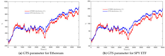
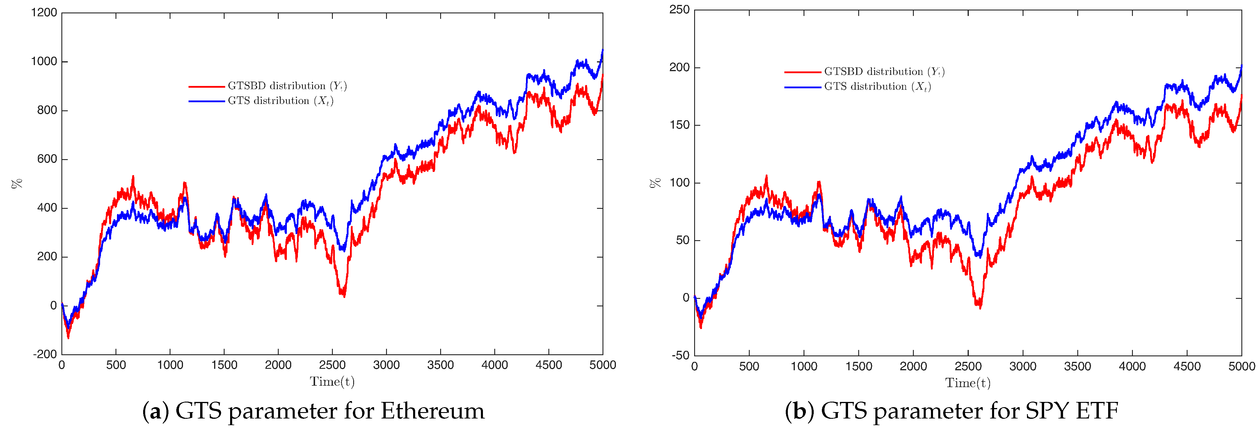
Based on the definition of the Lévy process introduced in Section 1 and the GTS parameter estimates reported in Table 1, Figure 1 was generated for the SPY ETF and ETH. When the random seed is held fixed, the BDLP and GTS processes exhibit highly synchronized movements, rising and falling together over time. Although both figures display similar temporal patterns, they differ in the magnitude of their fluctuations, which is consistent with the heavy-tailed and mean-reverting characteristics observed in similar time-series analyses [76]. This result suggests that the BDLP successfully reproduces the directional dynamics of the corresponding GTS process while exhibiting differences in scale.

Figure 1. Pathwise simulations of the background driving Lévy process (BDLP) versus GTS process.

5. Applications and Simulation of SPY ETF and Ethereum Price Dynamics Using an OU-Type Stationary Process

5.1. Algorithm for Simulating the Stationary Ornstein–Uhlenbeck-Type Process with a Background Driving Lévy Process

We recall the stationary Ornstein-Uhlenbeck-type process ${\left\{X\left(t\right)\right\}}_{t>0}$ and a background driving Lévy process (BDLP) ${\left\{Y\left(t\right)\right\}}_{t>0}$ independent of $X_0$, such that $X\left(t\right)\stackrel{d}{=}X$, as described in Theorem 2:

$$\begin{array}{c}\hfill X_t=e^{-\lambda t}{X}_0+{\int }_0^t{e}^{-\lambda (t-s)}d{Y}_{\lambda s}=e^{-\lambda t}{X}_0+{\int }_0^{\lambda t}{e}^{-\lambda t+s}d{Y}_s,\lambda >0.\end{array}$$

(41)

Lemma 1.

Let ${\left\{z\left(t\right)\right\}}_{t\ge 0}$ be a Lévy process, and let $f:D\to \mathbb{R}$ be a deterministic function satisfying the conditions required for the stochastic integral to exist. Define the stochastic integral of f with respect to z by:

$$f\ast z={\int }_{D}f\left(\tau \right)dz\left(\tau \right).$$

(42)

Then, the characteristic exponent of $f\ast z$ is given by:

$$log\mathbb{E}\left[e^{i\xi (f\ast z)}\right]={\int }_{D}log\mathbb{E}\left[e^{i\xi f\left(\tau \right)z\left(1\right)}\right]d\tau ,\xi \in \mathbb{R}.$$

(43)

Proof. 

See [47,72].    □

Theorem 8.

Let ${\left\{X\left(t\right)\right\}}_{t>0}$ be a stationary Ornstein–Uhlenbeck-type process with background driving Lévy process (BDLP) ${\left\{Y\left(t\right)\right\}}_{t>0}$, such that $X\left(t\right)\stackrel{d}{=}X$. Consider a discrete time horizon $t_0<t_1<t_2<\cdots <t_{n-1}<t_n$ with constant step size $\Delta =t_i-t_{i-1}$. The discrete-time version of the stationary process satisfies:

$$\begin{array}{c}\hfill X_{k\Delta }=e^{-\lambda \Delta }{X}_{(k-1)\Delta }+e^{-\lambda \Delta }{\int }_0^{\lambda \Delta }{e}^{s}d{Y}_s,\end{array}$$

(44)

where:

$$L:={\int }_0^{\lambda \Delta }{e}^{s}d{Y}_s$$

has characteristic exponent $\mathrm{\Psi }\left(\xi \right)=log\mathbb{E}\left[e^{i\xi L}\right]$ given by:

$$\begin{array}{cc}\hfill \mathrm{\Psi }\left(\xi \right)& =i\mu (e^{\lambda \Delta }-1)+{\mathrm{\Psi }}^{+}\left(\xi \right)+{\mathrm{\Psi }}^{-}\left(\xi \right),\hfill \\ \hfill {\mathrm{\Psi }}^{+}\left(\xi \right)& ={\alpha }_{+}\mathsf{\Gamma }(-{\beta }_{+})\left[{({\lambda }_{+}-i\xi e^{\lambda \Delta })}^{{\beta }_{+}}-{({\lambda }_{+}-i\xi )}^{{\beta }_{+}}\right],\hfill \\ \hfill {\mathrm{\Psi }}^{-}\left(\xi \right)& ={\alpha }_{-}\mathsf{\Gamma }(-{\beta }_{-})\left[{({\lambda }_{-}+i\xi e^{\lambda \Delta })}^{{\beta }_{-}}-{({\lambda }_{-}+i\xi )}^{{\beta }_{-}}\right].\hfill \end{array}$$

(45)

Proof. 

For $k=1$, substitute $t=\Delta$ into the continuous-time representation (Equation (41)) to obtain:

$$X_{\Delta }=e^{-\lambda \Delta }{X}_0+{\int }_0^{\lambda \Delta }{e}^{-\lambda \Delta +s}d{Y}_s.$$

Assume Equation (44) holds for a given k. For $k+1$, we compute:

$$\begin{array}{cc}\hfill X_{(k+1)\Delta }& =e^{-\lambda (k+1)\Delta }{X}_0+{\int }_0^{\lambda (k+1)\Delta }{e}^{-\lambda (k+1)\Delta +s}d{Y}_s\hfill \\ \hfill & =e^{-\lambda \Delta }\left(e^{-\lambda k\Delta }{X}_0+{\int }_0^{\lambda k\Delta }{e}^{-\lambda k\Delta +s}d{Y}_s\right)+{\int }_{\lambda k\Delta }^{\lambda (k+1)\Delta }{e}^{-\lambda (k+1)\Delta +s}d{Y}_s\hfill \\ \hfill & =e^{-\lambda \Delta }{X}_{k\Delta }+{\int }_0^{\lambda \Delta }{e}^{-\lambda \Delta +u}d{Y}_{u+\lambda k\Delta },\hfill \end{array}$$

where we set $u=s-\lambda k\Delta$. By stationarity of the increments of Y, we have $d{Y}_{u+\lambda k\Delta }\stackrel{d}{=}d{Y}_u$, and thus:

$$\begin{array}{c}\hfill X_{(k+1)\Delta }=e^{-\lambda \Delta }{X}_{k\Delta }+e^{-\lambda \Delta }{\int }_0^{\lambda \Delta }{e}^{u}d{Y}_u.\end{array}$$

(46)

Hence, Equation (44) holds for all k. Moreover, rearranging Equation (46) gives:

$$\begin{array}{c}\hfill L={\int }_0^{\lambda \Delta }{e}^{u}d{Y}_u=e^{\lambda \Delta }{X}_{(k+1)\Delta }-X_{k\Delta }.\end{array}$$

(47)

To find the characteristic exponent ($\mathrm{\Psi }\left(\xi \right)$) of L, we apply Lemma 1 on $\mathrm{\Psi }\left(\xi \right)$:

$$\mathrm{\Psi }\left(\xi \right)=log\mathbb{E}\left[e^{i\xi L}\right]={\int }_0^{\lambda \Delta }log\mathbb{E}\left[e^{i\xi e^{\tau }Y\left(1\right)}\right]d\tau ={\int }_0^{\lambda \Delta }log\phi \left(\xi e^{\tau }\right)d\tau ,$$

where $\phi$ is the characteristic function of $Y\left(1\right)$. Decomposing $log\phi$ into its positive and negative jump parts (see Equation (22)) yields:

$$\begin{array}{cc}\hfill \mathrm{\Psi }\left(\xi \right)& ={\int }_0^{\lambda \Delta }log\phi \left(\xi e^{\tau }\right)d\tau \hfill \\ \hfill & =i\mu (e^{\lambda \Delta }-1)+{\int }_0^{\lambda \Delta }log{\phi }^{+}\left(\xi e^{\tau }\right)d\tau +{\int }_0^{\lambda \Delta }log{\phi }^{-}\left(\xi e^{\tau }\right)d\tau .\hfill \end{array}$$

We define and compute ${\mathrm{\Psi }}^{+}\left(\xi \right)$:

$$\begin{array}{cc}\hfill {\mathrm{\Psi }}^{+}\left(\xi \right)& ={\int }_0^{\lambda \Delta }log{\phi }^{+}\left(\xi e^{\tau }\right)d\tau ={\alpha }_{+}\mathsf{\Gamma }(1-{\beta }_{+}){\int }_0^{\lambda \Delta }i\xi e^{\tau }{({\lambda }_{+}-i\xi e^{\tau })}^{{\beta }_{+}-1}d\tau \hfill \\ \hfill & ={\alpha }_{+}\mathsf{\Gamma }(-{\beta }_{+}){\left[{({\lambda }_{+}-i\xi e^{\tau })}^{{\beta }_{+}}\right]}_0^{\lambda \Delta }={\alpha }_{+}\mathsf{\Gamma }(-{\beta }_{+})\left[{({\lambda }_{+}-i\xi e^{\lambda \Delta })}^{{\beta }_{+}}-{({\lambda }_{+}-i\xi )}^{{\beta }_{+}}\right].\hfill \end{array}$$

Similarly, for the negative jump part:

$${\mathrm{\Psi }}^{-}\left(\xi \right)={\alpha }_{-}\mathsf{\Gamma }(-{\beta }_{-})\left[{({\lambda }_{-}+i\xi e^{\lambda \Delta })}^{{\beta }_{-}}-{({\lambda }_{-}+i\xi )}^{{\beta }_{-}}\right].$$

Summing the components gives Equation (43).    □

The Fourier transform generated by the characteristic exponent of Y in Equation (43), the probability density function (PDF) and the cumulative distribution function (CDF) have the following expressions:

$$F_L\left[f\right]\left(\xi \right)=e^{{\mathrm{\Psi }}^{-}\left(\xi \right)},f_L\left(y\right)={\displaystyle \frac{1}{2\pi }}{\int }_{-\infty }^{+\infty }{F}_L\left[f\right]\left(\xi \right)e^{iy\xi }d\xi ,F_L\left(y\right)={\int }_{-\infty }^{y}f\left(\xi \right)d\xi .$$

(48)

To compute the CDF, we use an advanced numerical inversion method—referred to as the enhanced FRFT-based inversion method [50,52,77]. This approach leverages the characteristic function of the generalized tempered stable (GTS) distribution and combines the Fast Fractional Fourier Transform (FRFT) with Newton–Cotes quadrature [78,79].

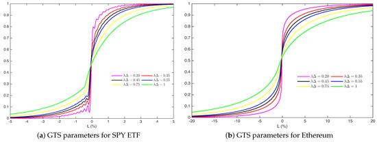
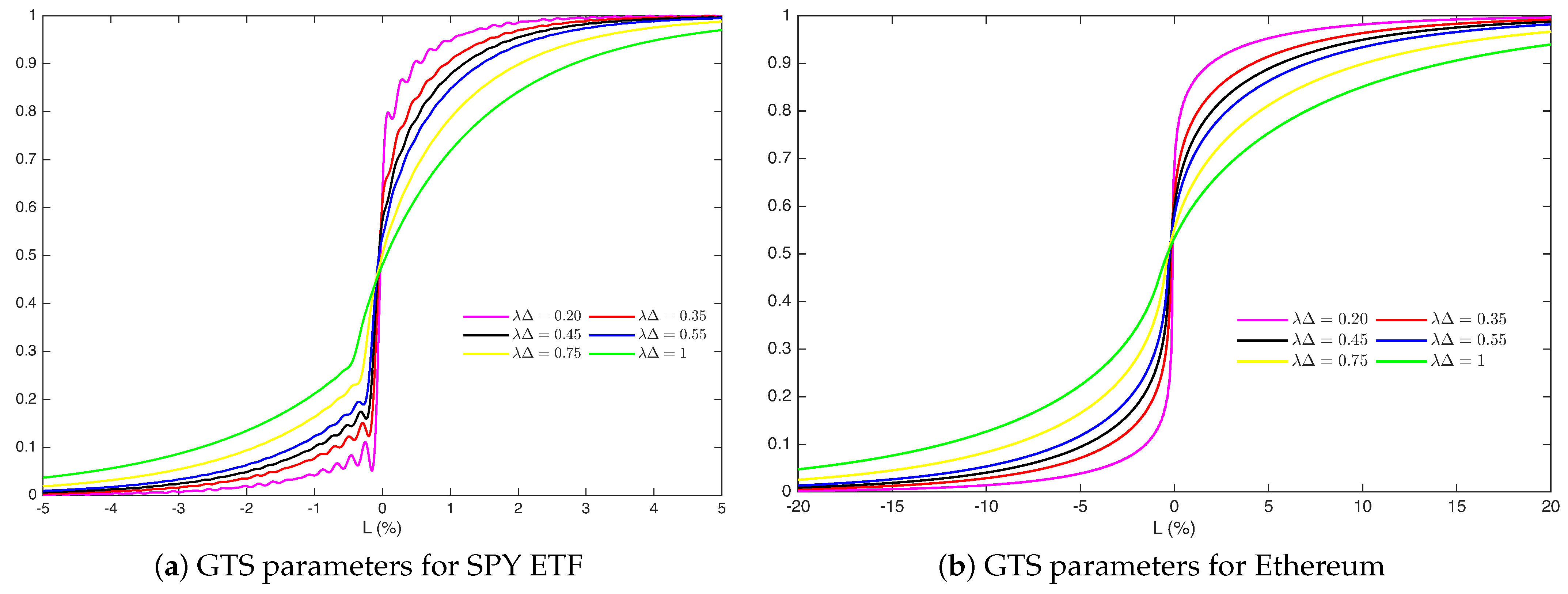
Using the GTS parameter estimates for the SPY ETF and Ethereum (reported in Table 1), Figure 2 plots the cumulative distribution functions (CDFs) of the random variable $L={\int }_0^{\lambda \Delta }{e}^{s}d{Y}_s$ across a range of small $\lambda \Delta$ values. As $\lambda \Delta$ rises from $0.2$ to 1, the six CDFs transition from a steep, tightly concentrated form around zero to a flatter, more diffuse distribution. This pattern reveals that lower $\lambda \Delta$ values restrict the variable to a much narrower support, whereas higher values broaden its spread, reflecting increased uncertainty or variability in the integrated process.

Figure 2. Cumulative distribution function (CDF) of $L={\int }_0^{\lambda \Delta }{e}^{s}d{Y}_s$.

5.2. Estimation of the Mean-Reversion Speed $\lambda$

The pattern, as depicted in Figure 2, provides empirical justification for the statistical estimation of the mean-reversion speed, as the calibration of the Ornstein–Uhlenbeck-type process to the SPY ETF and Ethereum processes critically depends on accurately recovering this parameter, which governs the persistence and variability of the integrated fluctuations. We use the rank correlation and the maximum likelihood methods; other methods for gaussian and non-gaussian can be explored in [80,81,82,83,84,85,86,87,88,89,90].

5.2.1. Mean-Reversion Speed ($\lambda$) Estimation via Rank Correlation

Lemma 2

(Rank correlation). Let $L={\left\{L_t\right\}}_{t\ge 0}$ be a Lévy process on $\mathbb{R}$ with characteristic triplet $(\gamma ,{\sigma }^2,M)$. Let

$${\widehat{q}}_k={\displaystyle \frac{1}{n-k}}{\displaystyle \sum _{j=0}^{n-k}}\mathbf{1}(L_j>0,L_{j+k}>0)$$

be an empirical estimator of $q_k=P(L_0>0,L_k>0)$. Then, for $k=1,2,\dots$,

$${\lambda }_k={\displaystyle \frac{H\left({\widehat{q}}_k\right)}{k}},$$

(49)

where:

$$H\left(\xi \right)=-log\left[sin\left(2\pi \left(\xi -\frac{1}{4}\right)\right)\right],\frac{1}{4}<\xi <\frac{1}{2}.$$

A proof of Lemma 2 can be found in [83,84].

Table 2 reports the empirical estimates of the rank correlation probabilities based on daily returns. For Ethereum, the estimate is $\widehat{q}1=23.85\%$, whereas for the SPY ETF, it is $\widehat{q}1=30.03\%$. Since the estimation procedure in Equation (49) requires $\widehat{q}1\in (25\%,50\%)$, the parameter $\lambda \Delta$ cannot be estimated for Ethereum. In contrast, the estimate for the SPY ETF satisfies the required condition, and $\widehat{\lambda \Delta }=2.30\%$, which indicates a stronger persistence in the sign dependence of SPY ETF returns compared with Ethereum.

Table 2. Estimation of the mean-reversion speed.

Label	Sample Size	Gauss Copula		Rank Correlation		Maximum Likelihood
		$\widehat{\mathit{rs}}({\mathit{X}}_{\mathbf{1}},{\mathit{X}}_{\mathbf{2}})$	$\widehat{\mathsf{\lambda }\Delta }$	${\widehat{\mathit{q}}}_{\mathbf{1}}(\%)$	$\widehat{\mathsf{\lambda }\Delta }$	${\displaystyle \frac{log\left(\mathit{L}(\mathsf{\lambda }\Delta )\right)}{\mathit{n}}}$	$\widehat{\mathsf{\lambda }\Delta }$
Ethereum	3255	−0.03985	3.17	23.85%		−4.55	2.26
SPY ETF	3661	−0.03140	3.41	30.03%	2.30	−4.33	2.94

Lemma 3

(Rank correlation for the Gauss copula). Let U and V have a bivariate Gaussian distribution. The sample rank correlation $\widehat{rs}(U,V)$ is the standard estimator of $rs(U,V)$ based on a sample ${(U_i,V_i)}_{1\le i\le n}$, defined as follows:

$$\widehat{rs}(U,V)={\displaystyle \frac{12}{n(n^2-1)}}{\displaystyle \sum _{i=1}^n}\left(\mathrm{rank}\left(U_i\right)-{\displaystyle \frac{n+1}{2}}\right)\left(\mathrm{rank}\left(V_i\right)-{\displaystyle \frac{n+1}{2}}\right).$$

Then, $rs(U,V)$ satisfies:

$$\rho (U,V)=2sin\left(6{\displaystyle \frac{rs(U,V)}{\pi }}\right),$$

(50)

where $\rho (U,V)$ is the Pearson correlation coefficient of U and V.

For a proof of Lemma 3, see [83,84].

Table 2 reports the empirical estimates of Spearman’s rank correlation based on daily returns. For Ethereum, the estimated rank correlation is $\widehat{rs}(U,V)=-0.03985$, whereas for the SPY ETF, it is $\widehat{rs}(U,V)=-0.03140$. Although both estimates are negative, their magnitudes are small, indicating only weak serial dependence between consecutive observations.

Applying the relationship in Equation (50) and using the absolute values of the estimated rank correlations, we obtain $\widehat{\lambda \Delta }=3.17$ for Ethereum and $\widehat{\lambda \Delta }=3.41$ for the SPY ETF. These relatively large estimates suggest a weak persistence in the dependence structure of both return series.

It should be emphasized, however, that the estimation procedure derived from Lemma 3 relies on the assumption that the dependence structure is adequately described by a Gaussian copula. Equivalently, it assumes that the transformed variables $(X_n,X_{n-1})$ follow a bivariate normal distribution. This assumption is questionable for both Ethereum and SPY ETF returns, which are well known to exhibit non-Gaussian features such as skewness, excess kurtosis, and heavy tails [4,5,52,77,91]. Consequently, the estimates obtained from Equation (50) should be interpreted with caution, as they may not fully capture the true dependence structure of the data.

5.2.2. Mean-Reversion Speed ($\lambda$) Estimation via Maximum Likelihood Method

Maximum likelihood estimation of the mean-reversion speed of Ornstein–Uhlenbeck processes and other parameters of the underlying distribution have been studied in the literature [86,92,93].

Let $\left(X_i\right)0\le i\le n$ denote a sample of observations from the stationary OU-type process. For a given value of $\lambda \Delta$, we construct the transformed sample $\left(L_i\right)0\le i\le n-1$ according to Equation (51) developed previously:

$$L_i=e^{\lambda \Delta }{X}_{(i+1)\Delta }-X_{i\Delta }=e^{\lambda \Delta }\left(X_{(i+1)\Delta }-X_{i\Delta }\right)+\left(e^{\lambda \Delta }-1\right)X_{i\Delta },$$

(51)

where $\lambda \Delta$ is the unknown parameter to be estimated.

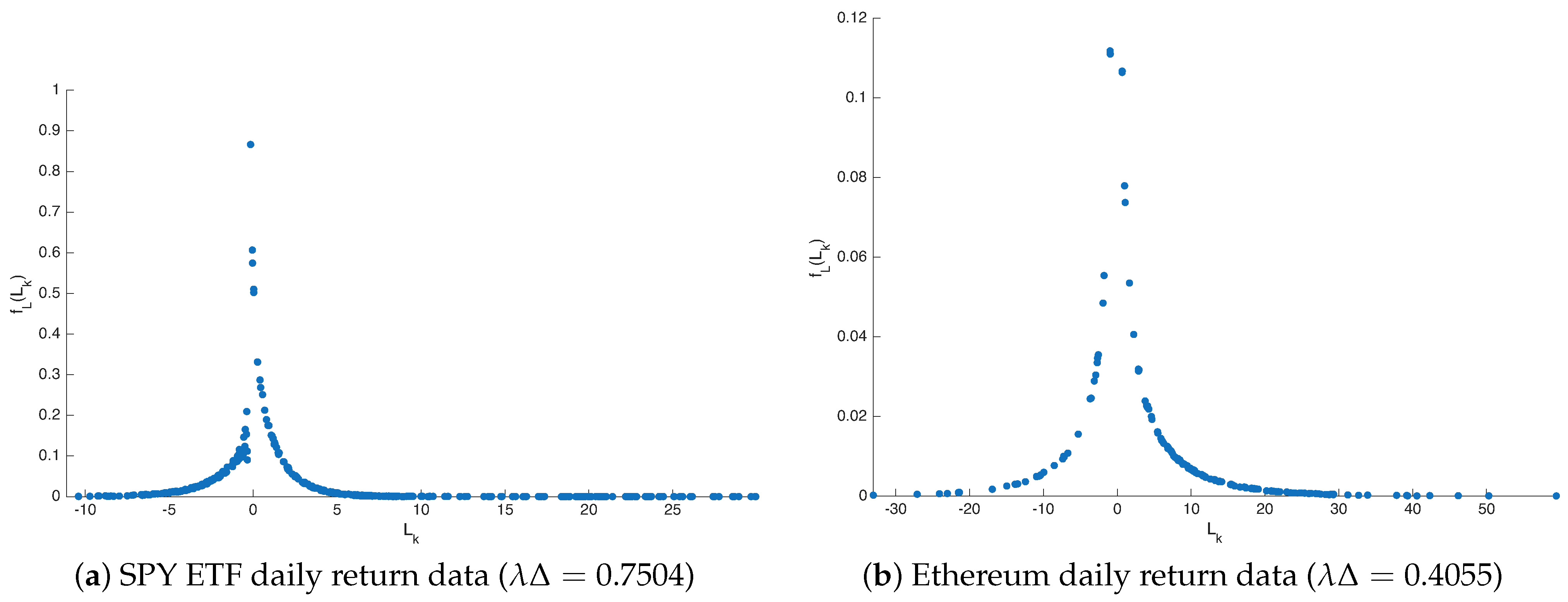
Figure 3 displays the empirical densities of the transformed variable $L_i$ obtained from Equation (51) using $\lambda \Delta =0.7504$ for the SPY ETF and $\lambda \Delta =0.4055$ for Ethereum. In both cases, the resulting distributions are highly concentrated around zero, indicating that relatively small values of $\lambda \Delta$ produce transformed samples with limited dispersion—see Figure 2.

Figure 3. Empirical density of the transformed variable L.

Assuming that ${\left(L_i\right)}_{0\le i\le n-1}$ can be approximated by an i.i.d. sample with density $f_L\left(y\right)$ in Equation (48), we define the estimate $\lambda$ by maximum likelihood (ML) by the following function:

$$log\left(ML(\lambda \Delta )\right)={\displaystyle \sum _{k=1}^{n-1}}log\left(f_L\left(L_k\right)\right).$$

(52)

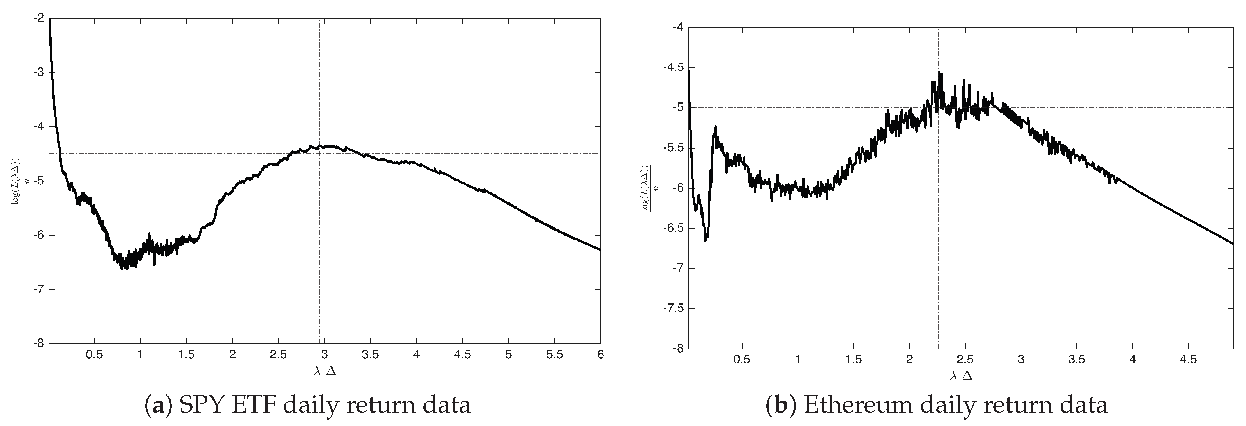
Figure 4 displays the log-likelihood function $log\left(ML(\lambda \Delta )\right)$ for the SPY ETF and Ethereum. The maximum of each curve determines the corresponding maximum likelihood estimate of the mean-reversion speed. The resulting estimates are $\widehat{\lambda \Delta }=2.94$ for the SPY ETF and $\widehat{\lambda \Delta }=2.26$ for Ethereum.

Figure 4. $log\left(ML(\lambda \Delta )\right)$.

Combining Figure 2 and Figure 4, we observe that values of $\lambda \Delta$ in the range $[0.2,1]$ provide a relatively poor fit to the data. Specifically, these values generate transformed samples whose empirical distributions are overly concentrated around zero and are associated with lower values of the log-likelihood function. In contrast, larger values of $\lambda \Delta$ lead to substantially higher likelihood values, suggesting a more appropriate representation of the dependence structure observed in both the SPY ETF and Ethereum return series.

5.3. Simulation of Ethereum and SPY ETF Return Dynamics Using the Ornstein–Uhlenbeck Process

To assess the ability of the Ornstein–Uhlenbeck-type model to reproduce the observed dynamics of financial returns, we simulate sample paths using the estimated parameters obtained in the previous section. The simulation procedure is summarized in Algorithm 1.

Algorithm 1 Simulation of the stationary Ornstein–Uhlenbeck-type process

Require:  $\lambda \Delta$; BDLP Y; discrete times $t_0<t_1<\cdots <t_n$ 1: $X_0\leftarrow x$                           ▹  Initialization 2: for $i=1$ to N do 3:       $a\leftarrow e^{-\lambda \Delta }$ 4:       $u_i\sim \mathcal{U}(0,1)$                  ▹ Uniform random number 5:       $y_i\leftarrow F_Y^{-1}\left(u_i\right)$                ▹ Inverse CDF method via (48) 6:       $X_{i\Delta }\leftarrow a{X}_{(i-1)\Delta }+y_i$ 7: end for

The stationary Ornstein–Uhlenbeck-type process ${\left(X_{k\Delta }\right)}_{k\ge 0}$ is employed to model the cumulative daily returns of the SPY ETF and Ethereum. Using the estimated parameters of the background driving Lévy process (BDLP), together with the maximum likelihood estimates of the mean-reversion parameter, simulated sample paths are generated and compared with the observed cumulative return series.

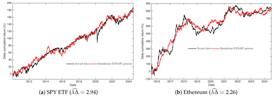
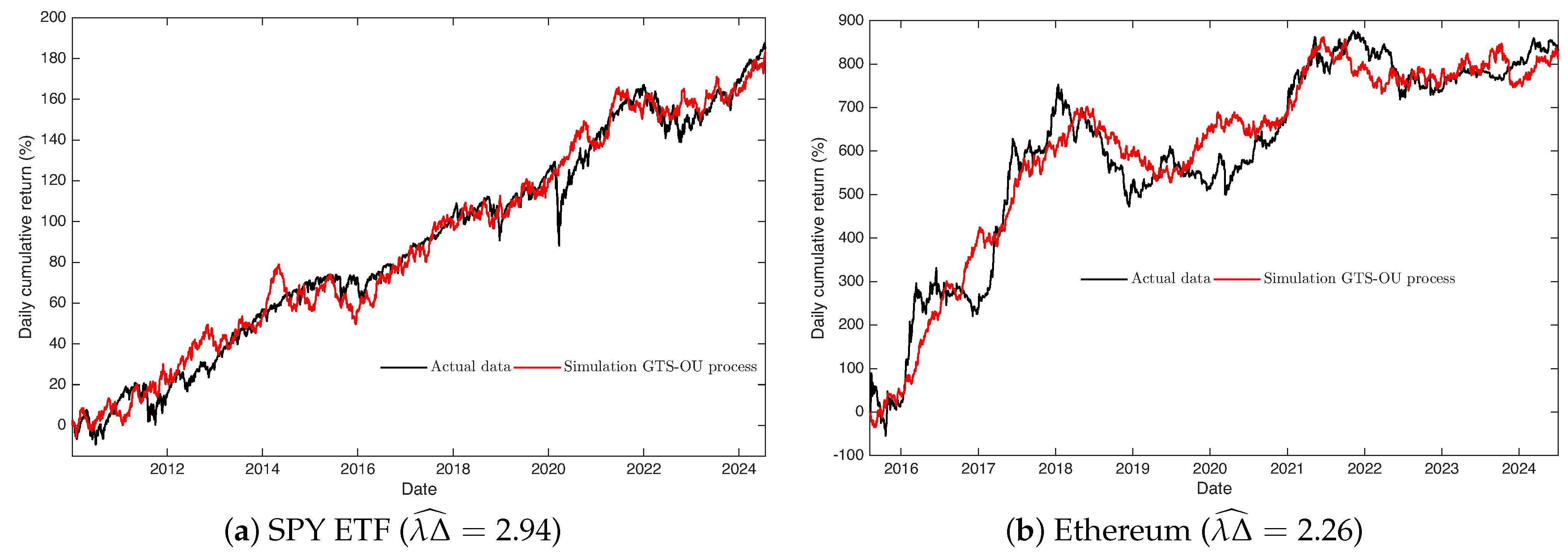
Figure 5 displays representative simulated trajectories together with the corresponding observed cumulative returns. In each panel, the simulated path is shown in red and the observed path in black. The simulations reproduce the overall upward trend exhibited by both assets while preserving the substantial short-term fluctuations characteristic of financial markets.

Figure 5. Observed and simulated cumulative daily return paths.

To complement the visual comparison, we consider the following error measures:

$$\begin{array}{cc}\hfill {\tau }_1^a& ={\int }_0^a\left(X\left(t\right)-\widehat{X}\left(t\right)\right)dt{R}_1^a={\displaystyle \frac{{\int }_0^a\left(X\left(t\right)-\widehat{X}\left(t\right)\right)dt}{{\int }_0^a\left|X\left(t\right)\right|dt}},\hfill \end{array}$$

(53)

$$\begin{array}{cc}\hfill {\tau }_2^a& ={\int }_0^a\left|X\left(t\right)-\widehat{X}\left(t\right)\right|dt{R}_2^a={\displaystyle \frac{{\int }_0^a\left|X\left(t\right)-\widehat{X}\left(t\right)\right|dt}{{\int }_0^a\left|X\left(t\right)\right|dt}}.\hfill \end{array}$$

(54)

The measure ${\tau }_1^a$ captures the signed cumulative error and may therefore reflect systematic overestimation or underestimation of the observed path. In contrast, ${\tau }_2^a$ measures the cumulative absolute deviation and provides a more direct assessment of the overall discrepancy between the simulated and observed trajectories. The corresponding relative measures $R_1^a$ and $R_2^a$ normalize these quantities and facilitate comparisons across assets.

The resulting error metrics are reported in Table 3.

Table 3. Error metrics comparing observed and simulated cumulative return paths.

Asset	Absolute Error		Relative Error
	${\mathsf{\tau }}_{\mathbf{1}}^{\mathit{a}}$	${\mathsf{\tau }}_{\mathbf{2}}^{\mathit{a}}$	${\mathit{R}}_{\mathbf{1}}^{\mathit{a}}$	${\mathit{R}}_{\mathbf{2}}^{\mathit{a}}$
$\mathbf{SPY} \mathbf{ETF}$	−41.22	230.09	−1.27%	7.08%
$\mathbf{ETHEREUM}$	−196.19	1551.47	−1.01%	7.98%

The error metrics reported in Table 3 indicate that the OU-type model provides a reasonable approximation of the cumulative return dynamics of both the SPY ETF and Ethereum. The relative absolute errors, $R_2^a=7.08\%$ for the SPY ETF and $R_2^a=7.98\%$ for Ethereum suggest that the simulated trajectories closely follow the observed return paths over the sample period. Although the model exhibits a slightly better fit for the SPY ETF, the difference in performance remains relatively small. The larger errors obtained for Ethereum are consistent with the higher volatility and more complex return behavior typically observed in cryptocurrency markets. Overall, the results suggest that the proposed OU-type framework is capable of capturing the principal features of both return series while maintaining a reasonable level of accuracy.

6. Conclusions

This paper has identified and characterized the background driving Lévy process (BDLP) associated with the Generalized Tempered Stable (GTS) distribution, which is a contribution to the theory of self-decomposable processes and their financial applications. The main theoretical result is the explicit derivation of the Lévy density (BDLD) and the characteristic exponent for the GTS background driving process, establishing that the GTS distribution is self-decomposable. Specifically, we demonstrated that the BDLD differs from the GTS Lévy measure but conserved the same Lévy process properties, such as infinity activity and finite variation. From a practical standpoint, we derived closed-form expressions for the characteristic exponent and cumulants of the GTS background driving distribution (GTSBD) and recovered the background driving of several well-known models as special cases, including the bilateral stable, bilateral Gamma, and Variance Gamma distributions. The theoretical framework was then applied to real-world financial data: daily returns of the SPY ETF and Ethereum prices from 2010 to 2024. Using maximum likelihood estimation and an enhanced FRFT-based inversion method, we calibrated the simulated stationary Ornstein–Uhlenbeck-type processes. Similar to the GTS distribution, the proposed GTSBD framework provides a rigorous and flexible mathematical foundation for modeling self-decomposable processes in finance. The simulation algorithm developed herein offers a practical tool for pricing, risk management, and scenario generation under non-Gaussian dynamics. Future work may extend this analysis in several directions: (i) applying the GTSBDL directly to high-frequency intraday data; and (ii) refining of the FRFT-based inversion for very small $\lambda \Delta$ regimes could improve numerical stability and broaden the applicability of the method.

References

- Cont, R. Empirical Properties of Asset Returns: Stylized Facts and Statistical Issues. Quant. Financ. 2001, 1, 223–236. [Google Scholar] [CrossRef]
- Kim, Y.S.; Rachev, S.T.; Bianchi, M.L.; Fabozzi, F.J. Financial Market Models with Lévy Processes and Time-Varying Volatility. J. Bank. Financ. 2008, 32, 1363–1378. [Google Scholar] [CrossRef] [Scilit]
- Bianchi, M.L.; Rachev, S.T.; Kim, Y.S.; Fabozzi, F.J. Tempered Infinitely Divisible Distributions and Processes. Theory Probab. Appl. 2011, 55, 2–26. [Google Scholar] [CrossRef] [Scilit]
- Nzokem, A.; Maposa, D. Heavy-Tail Risk in Traditional Versus Crypto Markets: A Q-Q Plot-Based Analysis. In Proceedings of the 2026 International Conference on Artificial Intelligence, Computer, Data Sciences and Applications (ACDSA), Boracay Island, Philippines, 5–7 February 2026; pp. 1–6. [Google Scholar] [CrossRef] [Scilit]
- Nzokem, A.; Maposa, D. Peakedness and Tail Heaviness in Crypto Returns: A Risk Management Perspective on Bitcoin and Ethereum. In Proceedings of the 2026 International Conference on Artificial Intelligence, Computer, Data Sciences and Applications (ACDSA), Boracay Island, Philippines, 5–7 February, 2026; pp. 1–6. [Google Scholar] [CrossRef] [Scilit]
- Nolan, J.P. Modeling with Stable Distributions. In Univariate Stable Distributions; Springer: Cham, Switzerland, 2020; pp. 25–52. [Google Scholar] [CrossRef] [Scilit]
- Borak, S.; Härdle, W.; Weron, R. Stable Distributions. In Statistical Tools for Finance and Insurance; Springer: Berlin/Heidelberg, Germany, 2005; pp. 21–44. [Google Scholar] [CrossRef] [Scilit] [PubMed]
- Fallahgoul, H.; Loeper, G. Modelling Tail Risk with Tempered Stable Distributions: An Overview. Ann. Oper. Res. 2021, 299, 1253–1280. [Google Scholar] [CrossRef] [Scilit]
- Kim, Y.S.; Roh, K.H.; Douady, R. Tempered Stable Processes with Time-Varying Exponential Tails. Quant. Financ. 2022, 22, 541–561. [Google Scholar] [CrossRef] [Scilit]
- Rosiński, J. Tempering Stable Processes. Stoch. Process. Appl. 2007, 117, 677–707. [Google Scholar] [CrossRef] [Scilit]
- Kim, Y.S.; Rachev, S.T.; Bianchi, M.L.; Fabozzi, F.J. A New Tempered Stable Distribution and its Application to Finance. In Proceedings of the Risk Assessment: Decisions in Banking and Finance; Bol, G., Rachev, S.T., Würth, R., Eds.; Springer: Berlin/Heidelberg, Germany, 2009; pp. 77–109. [Google Scholar]
- Boyarchenko, S.I.; Levendorskiĭ, S.Z. Non-Gaussian Merton-Black-Scholes Theory. In Advanced Series on Statistical Science & Applied Probability; World Scientific: Singapore, 2002; Volume 9. [Google Scholar] [CrossRef]
- Rosiński, J. Generalized tempered stable processes. Banach Cent. Publ. 2010, 90, 153–170. [Google Scholar] [CrossRef] [Scilit]
- Rosiński, J. Series Representations of Lévy Processes from the Perspective of Point Processes. In Lévy Processes: Theory and Applications; Barndorff-Nielsen, O.E., Resnick, S.I., Mikosch, T., Eds.; Birkhäuser: Boston, MA, USA, 2001; pp. 401–415. [Google Scholar] [CrossRef] [Scilit]
- Rachev, S.T.; Kim, Y.S.; Bianchi, M.L.; Fabozzi, F.J. Stable and Tempered Stable Distributions. In Financial Models with Lévy Processes and Volatility Clustering; Rachev, S.T., Kim, Y.S., Bianchi, M.L., Fabozzi, F.J., Eds.; The Frank J. Fabozzi Series; John Wiley & Sons: Hoboken, NJ, USA, 2011; Volume 187, pp. 57–85. [Google Scholar] [CrossRef] [Scilit]
- Küchler, U.; Tappe, S. Tempered Stable Distributions and Processes. Stoch. Process. Appl. 2013, 123, 4256–4293. [Google Scholar] [CrossRef] [Scilit]
- Küchler, U.; Tappe, S. Bilateral Gamma Distributions and Processes in Financial Mathematics. Stoch. Process. Their Appl. 2008, 118, 261–283. [Google Scholar] [CrossRef] [Scilit]
- Moutanabbir, K.; Ezin, H.P. A Large Class of Bilateral Distributions for Financial Applications. Methodol. Comput. Appl. Probab. 2025, 27, 63. [Google Scholar] [CrossRef] [Scilit]
- Xie, H.; Wang, S.; Lu, Z. The behavioral implications of the bilateral gamma process. Phys. A 2018, 500, 259–264. [Google Scholar] [CrossRef] [Scilit]
- Küchler, U.; Tappe, S. On the shapes of bilateral gamma densities. Stat. Probab. Lett. 2008, 78, 2478–2484. [Google Scholar] [CrossRef] [Scilit][Green Version]
- Nzokem, A.H. Gamma variance model: Fractional Fourier Transform (FRFT). J. Phys. Conf. Ser. 2021, 2090, 012094. [Google Scholar] [CrossRef] [Scilit]
- Nzokem, A.H.; Montshiwa, V.T. The Ornstein–Uhlenbeck Process and Variance Gamma Process: Parameter Estimation and Simulations. Thai J. Math. 2023, 21, 160–168. [Google Scholar]
- Nzokem, A.H. Fitting Infinitely divisible distribution: Case of Gamma-Variance Model. arXiv 2021, arXiv:2104.07580. [Google Scholar]
- Nzokem, A.H. Pricing European Options under Stochastic Volatility Models: Case of Five-Parameter Variance-Gamma Process. J. Risk Financ. Manag. 2023, 16, 55. [Google Scholar] [CrossRef] [Scilit]
- Drahokoupil, J. Variance Gamma process in the option pricing model. Ffa Work. Pap. 2021, 3, 2021.002. [Google Scholar]
- Madan, D.B.; Carr, P.P.; Chang, E.C. The variance gamma process and option pricing. Rev. Financ. 1998, 2, 79–105. [Google Scholar] [CrossRef] [Scilit]
- Nzokem, A.H. Five-Parameter Variance-Gamma Process: Lévy versus Probability Density. AIP Conf. Proc. 2024, 3005, 020030. [Google Scholar] [CrossRef] [Scilit]
- Carr, P.; Geman, H.; Madan, D.B.; Yor, M. Stochastic Volatility for Lévy Processes. Math. Financ. 2003, 13, 345–382. [Google Scholar] [CrossRef] [Scilit]
- Madan, D.B.; Yor, M. CGMY and Meixner Subordinators Are Absolutely Continuous with Respect to One-Sided Stable Subordinators. Financ. Stoch. 2008, 12, 359–380. [Google Scholar] [CrossRef] [Scilit]
- Nzokem, A.H.; Maposa, D. Fitting the Seven-Parameter Generalized Tempered Stable Distribution to Financial Data. J. Risk Financ. Manag. 2024, 17, 531. [Google Scholar] [CrossRef] [Scilit]
- Nzokem, A.H. European Option Pricing Under Generalized Tempered Stable Process: Empirical Analysis. arXiv 2023, arXiv:2304.06060. [Google Scholar]
- Nzokem, A.H. Simulation of Generalized Tempered Stable (GTS) Random Variates via Series Representations: A Case Study of Bitcoin and Ethereum. Preprint 2025, 2025080126. [Google Scholar] [CrossRef] [Scilit]
- Sabino, P.; Cufaro Petroni, N. Fast Simulation of Tempered Stable Ornstein–Uhlenbeck Processes. Monte Carlo Methods Appl. 2022, 28, 237–251. [Google Scholar] [CrossRef] [Scilit]
- Sabino, P. Exact Simulation of Normal Tempered Stable Processes of OU Type with Applications. Methodol. Comput. Appl. Probab. 2020, 22, 77–98. [Google Scholar] [CrossRef] [Scilit]
- Jurek, Z.J. On background driving distribution functions (BDDF) for some selfdecomposable variables. Math. Appl. 2021, 49, 85–109. [Google Scholar] [CrossRef] [Scilit]
- Jurek, Z.J. Background driving distribution functions and series representations for log-gamma self-decomposable random variables. Theory Probab. Appl. 2022, 67, 105–117. [Google Scholar] [CrossRef] [Scilit]
- Buchmann, B.; Lu, K.W.; Madan, D.B. Self-decomposability of Weak Variance Generalised Gamma Convolutions. Stoch. Process. Appl. 2020, 130, 630–655. [Google Scholar] [CrossRef] [Scilit]
- Carr, P.; Geman, H.; Madan, D.B.; Yor, M. Self-Decomposability and Option Pricing. Math. Financ. 2007, 17, 31–57. [Google Scholar] [CrossRef] [Scilit]
- Önalan, O. Pure-Jump Lévy Processes and Self-Decomposability in Financial Modeling. J. Math. Res. 2011, 3, 41–49. [Google Scholar] [CrossRef] [Scilit][Green Version]
- Nzokem, A.H. Self-Decomposable Laws Associated with General Tempered Stable (GTS) Distribution and Their Simulation Applications. arXiv 2024, arXiv:2405.16614. [Google Scholar]
- Hansen, B.G. Self-Decomposable Distributions and Branching Processes. In Memorandum COSOR; Technische Universiteit Eindhoven: Eindhoven, The Netherlands, 1989; Volume 8906. [Google Scholar]
- Barndorff-Nielsen, O.E. Probability Densities and Lévy Densities; Research Report MPS-RR 2000-18; Centre for Mathematical Physics and Stochastics (MaPhySto), Department of Mathematical Sciences, Aarhus University: Aarhus, Denmark, 2000. [Google Scholar]
- Barndorff-Nielsen, O.E. Superposition of Ornstein–Uhlenbeck type processes. Theory Probab. Appl. 2001, 45, 175–194. [Google Scholar] [CrossRef] [Scilit]
- Leonenko, N.N.; Pepelyshev, A. Simulation of supOU processes with specified marginal distribution and correlation function. Mod. Stoch. Theory Appl. 2026, 13, 225–254. [Google Scholar] [CrossRef] [Scilit]
- Barndorff-Nielsen, O.E.; Hubalek, F. Probability measures, Lévy measures and analyticity in time. Bernoulli 2008, 14, 764–790. [Google Scholar] [CrossRef] [Scilit]
- Barndorff-Nielsen, O.E.; Shephard, N. Non-Gaussian Ornstein–Uhlenbeck-based models and some of their uses in financial economics. J. R. Stat. Soc. Ser. B 2001, 63, 167–241. [Google Scholar] [CrossRef] [Scilit]
- Barndorff-Nielsen, O.E.; Shephard, N. Modelling by Lévy processess for financial econometrics. In Lévy Processes; Springer: Berlin/Heidelberg, Germany, 2001; pp. 283–318. [Google Scholar]
- Barndorff-Nielsen, O.E.; Shephard, N. Integrated OU Processes and Non-Gaussian OU-based Stochastic Volatility Models. Scand. J. Stat. 2003, 30, 277–295. [Google Scholar] [CrossRef] [Scilit]
- Barndorff-Nielsen, O.E.; Pérez-Abreu, V. Stationary and Self-Similar Processes Driven by Lévy Processes. Stoch. Process. Their Appl. 1999, 84, 357–369. [Google Scholar] [CrossRef] [Scilit][Green Version]
- Nzokem, A.H.; Maposa, D.; Seimela, A.M. Enhanced Fast Fractional Fourier Transform (FRFT) Scheme Based on Closed Newton-Cotes Rules. Axioms 2025, 14, 543. [Google Scholar] [CrossRef] [Scilit]
- Yang, X.; Tan, Q.; Wei, X.; Xiang, Y.; Yan, Y.; Jin, G. Improved Fast Fractional-Fourier-Transform Algorithm. J. Opt. Soc. Am. A 2004, 21, 1677–1681. [Google Scholar] [CrossRef] [Scilit] [PubMed]
- Nzokem, A.H.; Maposa. High-Performance Simulation of Generalized Tempered Stable Random Variates: Exact and Numerical Methods for Heavy-Tailed Data. Math. Comput. Appl. 2025, 30, 106. [Google Scholar] [CrossRef] [Scilit]
- Applebaum, D. Lévy Processes and Stochastic Calculus, 2nd ed.; Cambridge University Press: Cambridge, UK, 2009. [Google Scholar]
- Sato, K.I. Lévy Processes and Infinitely Divisible Distributions. In Cambridge Studies in Advanced Mathematics; Cambridge University Press: Cambridge, UK, 1999; Volume 68. [Google Scholar]
- Cont, R.; Tankov, P. Financial Modelling with Jump Processes; Chapman & Hall/CRC Financial Mathematics Series; Chapman & Hall/CRC Press: Boca Raton, FL, USA, 2003; p. 552. [Google Scholar]
- Itkin, A. A Brief Introduction to Lévy Processes. In Pricing Derivatives Under Lévy Models; Itkin, A., Ed.; Springer: New York, NY, USA, 2017; pp. 85–100. [Google Scholar] [CrossRef] [Scilit]
- Gnedenko, B.V.; Kolmogorov, A.N. Limit Distributions for Sums of Independent Random Variables; Addison-Wesley: Cambridge, MA, USA, 1954. [Google Scholar]
- Feller, W. An Introduction to Probability Theory and Its Applications, 2nd ed.; Wiley: New York, NY, USA, 1971; Volume 2. [Google Scholar]
- Jurek, Z.J.; Vervaat, W. An Integral Representation for Selfdecomposable Banach Space Valued Random Variables. Z. Wahrsch. Verw. Geb. 1983, 62, 247–262. [Google Scholar] [CrossRef] [Scilit]
- Jurek, Z.J. Series of independent exponential random variables. In Proceedings of the 7th Japan-Russia Symposium on Probability Theory and Mathematical Statistics, Tokyo, Japan, 26–30 July 1995; World Scientific: Singapore, 1996; pp. 174–182. [Google Scholar]
- Jurek, Z.J. Some definite integrals arising from selfdecomposable characteristic functions. Lith. Math. J. 2023, 63, 291–304. [Google Scholar] [CrossRef] [Scilit]
- Uhlenback, G.; Ornstein, L. On the theory of the Brownian motion. Phys. Rev. 1930, 36, 823–841. [Google Scholar] [CrossRef] [Scilit]
- Barndorff-Nielsen, O.E.; Jensen, J.L.; Sørensen, M. Some stationary processes in discrete and continuous time. Adv. Appl. Probab. 1998, 30, 989–1007. [Google Scholar] [CrossRef] [Scilit]
- Barndorff-Nielsen, O.E.; Shephard, N. Econometric Analysis of Realised Volatility and its Use in Estimating Lévy-Based Non-Gaussian OU Type Stochastic Volatility Models. J. R. Stat. Soc. Ser. B 2002, 64, 253–280. [Google Scholar] [CrossRef] [Scilit]
- Sato, K.I. Basic Results on Lévy Processes. In Lévy Processes: Theory and Applications; Barndorff-Nielsen, O.E., Mikosch, T., Resnick, S.I., Eds.; Birkhäuser: Boston, MA, USA, 2001; pp. 1–37. [Google Scholar] [CrossRef] [Scilit]
- Kyprianou, A.E. Fluctuations of Lévy Processes with Applications: Introductory Lectures; Springer: Berlin, Germany, 2014. [Google Scholar]
- Tankov, P. Financial Modeling with Lévy Processes; Institute of Mathematics of the Polish Academy of Sciences (IMPAN): Warsaw, Poland, 2010; p. 101. [Google Scholar]
- Nzokem, A.H.; Maposa, D. Bitcoin versus S&P 500 Index: Return and Risk Analysis. Math. Comput. Appl. 2024, 29, 44. [Google Scholar] [CrossRef] [Scilit]
- Hall, W.J.; Oakes, D. A Course in the Large Sample Theory of Statistical Inference; CRC Press: New York, NY, USA, 2023. [Google Scholar]
- Lehmann, E.L. Elements of Large-Sample Theory. In Springer Texts in Statistics; Springer: New York, NY, USA, 1999. [Google Scholar]
- Nzokem, A.H.; Montshiwa, V.T. Fitting Generalized Tempered Stable distribution: Fractional Fourier Transform (FRFT) Approach. arXiv 2022, arXiv:2205.00586. [Google Scholar]
- Barndorff-Nielsen, O.E.; Shephard, N. Financial Volatility, Lévy Processes and Power Variation. 2002. Available online: https://www.olsendata.com/data_products/client_papers/papers/200206-NielsenShephard-FinVolLevyProcessPowerVar.pdf (accessed on 19 June 2026).
- Qu, Y.; Dassios, A.; Zhao, H. Exact Simulation of Ornstein–Uhlenbeck Tempered Stable Processes. J. Appl. Probab. 2021, 58, 347–371. [Google Scholar] [CrossRef] [Scilit]
- Sabino, P. Exact simulation of normal tempered stable processes of OU type with applications. Stat. Comput. 2022, 32, 81. [Google Scholar] [CrossRef] [Scilit]
- Kendall, M.G. The Advanced Theory of Statistics, 2nd ed.; Charles Griffin and Company: London, UK, 1946. [Google Scholar]
- Raubitzek, S.; Schrittwieser, S.; Goldenits, G.; Schatten, A.; Mallinger, K. Mean Reversion and Heavy Tails: Characterizing Time-Series Data Using Ornstein–Uhlenbeck Processes and Machine Learning. Sensors 2026, 26, 1263. [Google Scholar] [CrossRef] [Scilit] [PubMed]
- Nzokem, A.; Mopasa, D. Exact Simulation for General Tempered Stable Random Variates: Review and Empirical Analysis. In Proceedings of the 2025 International Conference on Artificial Intelligence, Computer, Data Sciences and Applications (ACDSA); IEEE: New York, NY, USA, 2025; pp. 1–6. [Google Scholar] [CrossRef] [Scilit]
- Nzokem, A.H. Numerical Solution of a Gamma-Integral Equation Using a Higher Order Composite Newton-Cotes Formulas. J. Phys. Conf. Ser. 2021, 2084, 012019. [Google Scholar] [CrossRef] [Scilit]
- Nzokem, A.H. Stochastic and Renewal Methods Applied to Epidemic Models. Ph.D. Thesis, York University, Toronto, ON, USA, 2020. [Google Scholar]
- Trajanovski, P.; Jolakoski, P.; Zelenkovski, K.; Iomin, A.; Kocarev, L.; Sandev, T. Ornstein-Uhlenbeck process and generalizations: Particle dynamics under comb constraints and stochastic resetting. Phys. Rev. E 2023, 107, 054129. [Google Scholar] [CrossRef] [Scilit] [PubMed]
- Maller, R.A.; Müller, G.; Szimayer, A. Ornstein–Uhlenbeck processes and extensions. In Handbook of Financial Time Series; Springer: Berlin/Heidelberg, Germany, 2009; pp. 421–437. [Google Scholar]
- Holý, V.; Tomanová, P. Estimation of Ornstein–Uhlenbeck Process Using Ultra-High-Frequency Data with Application to Intraday Pairs Trading Strategy. Ann. Oper. Res. 2025, 1–35. [Google Scholar] [CrossRef] [Scilit]
- McNeil, A.J.; Frey, R.; Embrechts, P. Quantitative Risk Management: Concepts, Techniques and Tools, revised ed.; Princeton University Press: Princeton, NJ, USA, 2015. [Google Scholar]
- Borovkov, K.A.; Decrouez, G. Ornstein–Uhlenbeck Type Processes with Heavy Distribution Tails. Theory Probab. Appl. 2013, 57, 396–418. [Google Scholar] [CrossRef] [Scilit]
- Bao, Y.; Ullah, A.; Wang, Y. Distribution of the Mean Reversion Estimator in the Ornstein–Uhlenbeck Process. Econom. Rev. 2017, 36, 1039–1056. [Google Scholar] [CrossRef] [Scilit]
- Yu, J. Bias in the Estimation of the Mean Reversion Parameter in Continuous Time Models. J. Econom. 2012, 169, 114–122. [Google Scholar] [CrossRef] [Scilit]
- Baviera, R.; Manzoni, P. Fast and General Simulation of Lévy-driven Ornstein–Uhlenbeck Processes for Energy Derivatives. J. Comput. Appl. Math. 2026, 487, 117768. [Google Scholar] [CrossRef] [Scilit]
- Hu, Y.; Nualart, D. Parameter estimation for fractional Ornstein–Uhlenbeck processes. Stat. Probab. Lett. 2010, 80, 1030–1038. [Google Scholar] [CrossRef] [Scilit]
- Mariani, M.C.; Asante, P.K.; Kubin, W.; Tweneboah, O.K.; Beccar-Varela, M. Determining the Background Driving Process of the Ornstein–Uhlenbeck Model. Electron. J. Differ. Equ. 2023, 193–207. [Google Scholar] [CrossRef] [Scilit]
- Stein, J.; Medino, A.V.; de Souza, R.M.; Lopes, S.R.C. A Generalization of the Ornstein-Uhlenbeck Process: Theoretical Results, Simulations and Estimation. In Time Series and Wavelet Analysis; Chiann, C., Pinheiro, d.S., Toloi, A., Eds.; Springer: Cham, Switzerland, 2024; Chapter 6. [Google Scholar] [CrossRef] [Scilit]
- Nzokem, A.H. Comparing Bitcoin and Ethereum Tail Behavior via QQ Analysis of Cryptocurrency Returns. arXiv 2025, arXiv:2507.01983. [Google Scholar]
- Valdivieso, L.; Schoutens, W.; Tuerlinckx, F. Maximum Likelihood Estimation in Processes of Ornstein–Uhlenbeck Type. Stat. Inference Stoch. Process. 2009, 12, 1–19. [Google Scholar] [CrossRef] [Scilit]
- Bianchi, M.L.; Rachev, S.T.; Fabozzi, F.J. Tempered Stable Ornstein–Uhlenbeck Processes: A Practical View. Commun. Stat. Simul. Comput. 2011, 40, 1235–1255. [Google Scholar] [CrossRef] [Scilit]
Disclaimer/Publisher’s Note: The statements, opinions and data contained in all publications are solely those of the individual author(s) and contributor(s) and not of MDPI and/or the editor(s). MDPI and/or the editor(s) disclaim responsibility for any injury to people or property resulting from any ideas, methods, instructions or products referred to in the content. |
© 2026 by the authors. Licensee MDPI, Basel, Switzerland. This article is an open access article distributed under the terms and conditions of the Creative Commons Attribution (CC BY) license.