


Abstract
In this article, we employ a fractional version of the radius of curvature in Euler’s equation for column buckling, enabling us to derive a fractional differential equation in the Caputo sense. We solve this equation and demonstrate that for certain values of the fractional parameter, there exists a critical buckling force. Additionally, we provide a numerical scheme for accurately approximating this critical force.
1. Introduction
Although the origins of fractional calculus are quite old (around 1675), its theoretical development and, above all, its applications are relatively recent. See, for example, [1,2,3,4]. In many applications, fractional models are obtained by replacing the integer-order of the derivative in the original model with a fractional one. However, it has recently been observed that introducing an additional parameter, namely the fractional index, does not necessarily improve the resulting model; see [5,6,7,8,9,10]. Motivated by this observation, the purpose of the present work is to study the deflection of a column by deriving the governing fractional equation from a fractional approximation of the radius of curvature, rather than from a purely formal replacement of derivatives.
The analysis of buckling in materials, particularly in columns, is of crucial importance in applied mathematics and structural mechanics due to its numerous practical applications. This study is especially relevant in the construction industry, where the buckling of columns made from steel, aluminum, or plastic materials plays a key role. Similarly, this area of research is significant in other sectors, such as aviation and the automotive industries, among others. For further exploration of this topic, we refer the reader to [11,12,13] and the references therein.
Recent studies have shown that fractional calculus is not limited to abstract generalizations, but also provides useful tools in mechanics and structural stability. Fractional-order models have been used in continuum mechanics and materials modeling to describe nonlocal and size-dependent effects; see, for example, [14]. Moreover, fractional formulations have recently been applied to structural stability and buckling problems; see [15]. These works provide a relevant context for the present paper. In contrast with approaches based mainly on replacing classical derivatives with fractional ones, our model is obtained from a fractional approximation of the radius of curvature in Euler’s column theory.
The main novelty of this work is therefore geometric in nature: the fractional model is derived from the curvature law itself. This construction leads to a Caputo-type fractional differential equation and provides a new analytical treatment of the buckling condition through the first positive root of the associated solution. An important advantage of this formulation is that it extends the classical Euler model in a consistent way, recovers the standard case when , and reveals a threshold behavior in the existence of the critical load that does not appear in the classical setting.
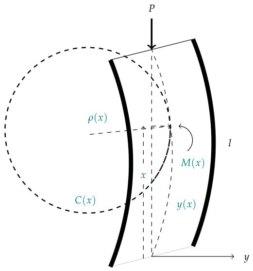
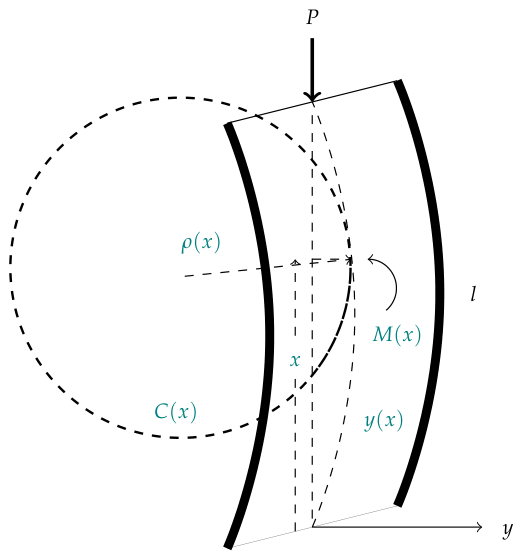
Suppose we have a beam of length l with one flexible end resting on the ground and a force P applied to the other flexible end. Under certain assumptions on the beam, the well-known Euler equation (see [16]) states that at a point x, the external moment of the deflected beam is inversely proportional to the radius of curvature . symbols,
where E is the Young’s modulus of the material and I denotes the second moment of inertia of the cross-sectional area. The displacement of the beam at point is represented by , which corresponds to the elastic curve of the beam (refer to Figure 1).
Figure 1.
The elastic curve and the osculating circle .
Assuming a scheme like the one presented in Figure 1, we know (see [17]) that the external moment is given by . To introduce the fractional component, , into the study of beam deflection, we work with the radius of curvature, . Indeed, through a detailed analysis based on the Caputo fractional derivative and on a fractional approximation of the radius of curvature, as discussed in Section 2, we derive the fractional differential equation:
The fractional parameter should be interpreted here as an effective index measuring the departure from the classical local Euler description. In the present formulation, arises from the fractional approximation of the radius of curvature, so its most immediate meaning is geometric. The limiting case recovers the standard curvature law, whereas introduces a nonclassical correction through a fractional curvature operator. Since this paper is conceptual and does not include experimental calibration, we do not assign to a unique physical mechanism. Rather, it is treated as a compact parameter encoding nonlocal or nonclassical effects that are not captured by the ideal homogeneous Euler column model.
Currently, there is a wide variety of fractional derivatives available (see [18]). Among the classical ones are the Riemann-Liouville, Grünwald-Letnikov, Caputo, Riesz, and Marchaud derivatives, to name a few (see [19,20], or [21]). In this work, we adopt the Caputo derivative because the Caputo derivative of a constant is zero, which is consistent with the classical geometric interpretation underlying the model. Moreover, it allows the fractional differential equation to be formulated with standard initial conditions such as and , exactly as in the classical formulation. This makes the Caputo framework particularly suitable for deriving and analyzing the fractional counterpart of Euler’s column equation considered here (see (15)).
The key point in our derivation is that, in the fractional setting, the classical differential increment cannot be transferred directly. Therefore, instead of postulating the fractional equation by replacing derivatives in Euler’s model, we use a linear approximation of the arc associated with the curvature radius , as indicated in (8). This procedure leads to the fractional model of column buckling considered in this paper.
The critical buckling force is given by
where denotes the first positive zero of the solution of Equation (2). In particular, if then , which coincides with the classical case (see [17]). Thus, the main complexity lies in the calculation of . According to our literature review, there are no precedents of studies that have identified positive roots for solutions of fractional differential equations in the Caputo context considered here. Beyond its practical motivation, this aspect of the work introduces analytical techniques that may also be useful in the study of solutions represented by power series.
To determine , or more precisely, to find an approximation of , we note that the function is the uniform limit, over compact intervals, of certain polynomials. Assuming there is a polynomial that meets specific conditions (see Assumption 1), we demonstrate that has a positive root, as detailed in Theorem 2. Furthermore, if we impose additional regularity conditions on (see Assumption 2), then for a given error , we can obtain an approximation of that differs by less than units, as outlined in Theorem 3. Thus, we obtain an approximation of the critical force P, as seen in Equation (3).
Our numerical experiments suggest that does not exist for all values of the index . Specifically, we observe that for , the function lacks positive roots, whereas the opposite occurs for . This indicates a threshold phenomenon in the existence of the critical buckling force predicted by the fractional model. Additional qualitative features of the fractional solutions, including their symmetry properties and the possible use of
are discussed in the numerical section.
The paper is structured as follows. In Section 2, we derive the radius of curvature involving the fractional index . In Section 3, Theorem 1 presents the solution of Equation (2). Assuming that can be approximated by a polynomial, we establish in Theorem 2 that has a positive root. Additionally, Theorem 3 provides a method for approximating such a root. In Section 4, we demonstrate that for , the function does not have a positive root, whereas for , it does. Finally, Section 5 contains some concluding comments.
2. A Fractional Approximation of the Radius of Curvature
Let us start by remembering the definition of the Caputo fractional derivative, for . The left-side Caputo fractional derivative of a smooth function is defined as
where and denotes the integer part of . It is known (see [21] or [20]) that Caputo’s fractional derivative is linear and satisfies
Let us assume the function has second derivative. Given a point , we know that the radius of curvature, , of the osculating circle, , at is given by
If the slope is small enough that its square can be disregarded compared to 1, then we have
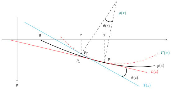
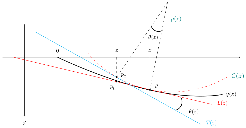
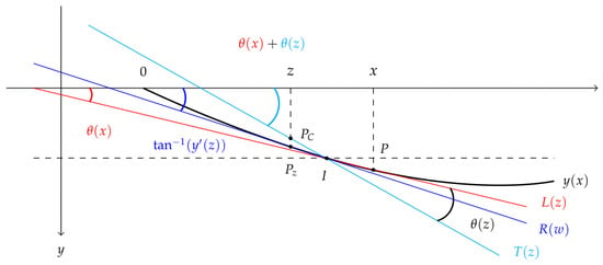
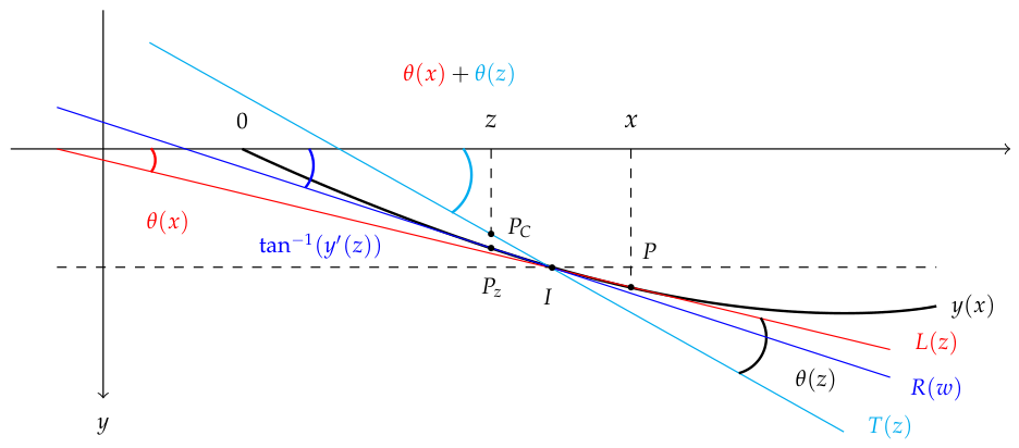
The traditional derivation of the radius of curvature relies on differentials, a concept not directly translatable to the fractional realm. To approximate (6) in this context, we adopt the following approach. Let such that . Then, the equation
describes the tangent line to y at the point . Now, consider a point z close to x, and suppose, for example, . Denote by the angle between the segments associated with z and x, and denote by the tangent line at on the osculating circle (see Figure 2).
Figure 2.
The osculating circle .
Let us denote by the length of the arc corresponding to a circle with angle and by the radius of curvature at x, then
We adhere to the convention of considering the angle positive if it is measured in the clockwise direction. If z approaches x from the left, then is negative. Given that z is close to x, the points and are nearly coincident. Consequently, the magnitude of is approximately the length of the segment from to :
Utilizing the linearity property of Caputo’s fractional derivative and referencing Equation (4), with , , and , we derive
Now, let us focus on the right-hand side of (7), specifically addressing the function . Let be the angle of the line L. Drawing a line parallel to the x-axis that passes through the point I, where the lines L and T intersect, we see that the angle of line T is . Let R be the tangent line at the point ,
Since and because the elastic curve is a smooth function, then . Moreover, the angle of line T is approximately equal to the angle of line R (see Figure 3):
Figure 3.
The tangent lines. In blue is the tangent line at .
Since , then . We know that for small angles x, given in radians, . Using this and (10) we deduce that
The observation that the fractional derivative of constant functions is zero, as indicated in Equation (4), results in the following equation
At this stage, x is regarded as an arbitrary but fixed point, and the fractional differentiation is taken with respect to the auxiliary variable z. Therefore, in the identity
the quantity is constant with respect to z. Evaluating the resulting relation at , we obtain
As in the previous case, if the square of is significantly smaller than 1, we arrive at the approximation
This is similar to (6), but with the additional factor of .
3. Solving the Fractional Differential Equation
For , we define the parameter as follows
where E, I and P are positive constants. Our first aim is to solve the fractional differential equation
subject to the initial conditions
An intuitive way to understand the influence of the fractional order is the following. The parameter changes the structure of the differential operator in Equation (14), and hence changes the series representation of the solution . This affects the way in which the solution bends and approaches the horizontal axis. Therefore, unlike in the classical case, the existence of a first positive zero is no longer automatic and may depend strongly on the value of . As we will see, this explains why the critical buckling load exists only for certain ranges of the fractional parameter.
Given the physical constraints of the problem, we have . The initial condition for the derivative, denoted as , remains undetermined. Identifying is crucial for calculating the critical load. We start by seeking the solution to the initial value problem (14) and (15).
Theorem 1.
Let us set
where
Proof.
By applying the root criterion, we can ascertain that the power series in (16) converges absolutely over . This conclusion is drawn from the observation that
On the other hand, given that and
yield . Now, let us calculate the fractional derivative of ,
This result confirms the desired equality (14). □
For we define
Then the solution of (14) can be expressed as
We know that , then or . If , the column has not bent at all. On the other hand we have . Thus we need to find the smallest positive root of the function in order to obtain the critical load (force).
We denote the smallest positive root of the polynomial as . The existence of depends on whether n is an odd or even integer. For odd integers n, a root always exists. This is due to the intermediate value theorem, as a polynomial of odd degree must cross the x-axis at least once, ensuring at least one real root. However, for even integers n, the existence of such a root is not guaranteed.
Lemma 1.
Let α be in . The following functions defined on
are both and strictly increasing functions.
Proof.
To verify the monotonicity property, we will use the relation for . Applying this, we have
and
Thus, the desired property is clearly established. □
In what follows we require the following hypothesis.
Assumption 1.
Let us suppose there is a polynomial , with an even integer, such that it has a first positive root that satisfies the inequality
Lemma 2.
For each we have on .
Proof.
Given that the series below converges absolutely, we can rearrange the terms as follows
The monotonicity property of f, as stated in Lemma 1, and the condition imply
therefore, on .
Now, let us consider
For and , Lemma 1 implies
thus on . This completes the proof of the desired inequalities. □
We now turn our attention to a result concerning the monotonicity of the sequence . This investigation will help us understand how the sequence behaves as n varies, particularly in terms of its increasing or decreasing nature.
Lemma 3.
Let n and m be two positive integers such that . If m and n are even integers, then on . Additionally, if m and n are odd integers, then on .
Proof.
If n and m are even integers, with , then
For we have, from Lemma 1,
Therefore on .
Now, let m and n be two odd integers such that , then
Again, by Lemma 1 we have, for ,
therefore on . This proves the result. □
Note that and
since . Therefore, by the intermediate value theorem, there exists a root such that . We are now equipped to demonstrate the existence of a positive root for .
Theorem 2.
The function has a first positive root, and this root is located in .
Proof.
By taking in Lemma 2, we deduce that . Given that , the intermediate value theorem guarantees that must have a root in the interval . Let us denote by the first positive root of .
For each , Lemma 2 implies that . Therefore, has a root , and it follows that . Consequently, we obtain a sequence . This sequence is increasing; indeed, Lemma 3 indicates that , implying that . Let us define
We aim to show that . To do this, suppose that . Take an . By the definition of we have for . The continuity of implies
By Weierstrass’s M-test, the sequence converges uniformly over compact intervals. Hence, there exists such that for all ,
In particular, we can choose a sufficiently large odd integer n such that . The preceding inequality then leads to
This contradiction implies the desired equality, . □
We now propose a method to approximate the first positive root of . To this end, we introduce the following hypothesis.
Assumption 2.
We assume that for x on and that
Theorem 3.
If , regardless of whether n is even or odd, the existence of the first root, , of is guaranteed. Furthermore, the sequence satisfies the condition
Given an we can find an integer (existence ensured by the first part of this theorem) such that
then
Consequently, this provides an approximation to the first positive root, , of with an error margin of at most ε units.
Proof.
For each , we have . Note that Lemma 3 implies . Therefore, has a minimal positive root, , for all . Additionally, Lemma 2 indicates that in and since , it follows that . Furthermore, according to Lemma 3 we have , implying . Consequently, the sequence is monotonically decreasing and bounded below by . This leads to the conclusion that
Now, let us demonstrate that . Suppose, for contradiction, that . First, let us consider the expression
Using the monotonicity property of g as established in Lemma 1, for and , we have
which implies that . The continuity of implies the existence of a such that , for all . Let us take an . Since we can find a large enough even integer n such that
which implies that . Given that and by applying the intermediate value theorem, it follows that . However, this conclusion is contradictory, as we have established that for all even integer n. Consequently, it must be that .
Given , there exists an integer , such that if and , with i an odd integer and j an even integer, then
Consequently, if , we have
Thus, the limit as expressed in (17) is effectively established. □
In this context, we have found an approximation, , of . Therefore, if , it follows that
From this, we obtain an approximate critical load, see the Formula (3).
Assumptions 1 and 2 are analytical and numerical admissibility conditions on the polynomial approximations , not physical hypotheses on the material. Together, they ensure that the first positive root of the limit function can be detected and approximated from the roots of suitable truncations.
Assumption 1 requires an even-degree truncation to possess a first positive root satisfying a quantitative inequality. This guarantees that the truncation captures the relevant sign change, which is essential for proving that admits a root in the interval .
Assumption 2 complements this with a local monotonicity condition on over and an additional quantitative bound. Jointly, these conditions ensure the numerical stability of the truncated roots and enable Theorem 3 to deliver a controlled approximation of . In short, Assumptions 1 and 2 are practical criteria ensuring that the truncation is sufficiently faithful near the root of interest, as the next section makes clear.
4. Some Illustrative Examples
In this section, we explore two illustrative examples that clarify the concepts. It should be noted that the approximation of the first positive root is performed in two steps. First, Theorem 3 provides the theoretical approximation criterion: given , an index is chosen such that
which guarantees that
Therefore, calculating the first positive root of using the first positive root of the polynomial already has an explicit error bound.
Once the polynomial is fixed, its first positive root is calculated numerically using the bisection method. The continuity of the polynomial implies that the bisection method is convergent. Furthermore, in each iteration, the interval containing the root is halved, so the midpoint approximation is numerically stable and its error is controlled by the length of the current interval.
In our implementation, the calculation ended when the numerical value of the root stabilized on the order of . In this way, the overall approximation of combines the theoretical estimate provided by Theorem 3 with the numerical precision of the bisection routine.
4.1. Non-Existence of an Even Degree Polynomial with a Positive Root
In this subsection, we will take and . Observe that
According to Lemma 1, for ,
therefore, on . This particularly implies that if
then does not have a root in .
The Table 1 displays the first positive root of the polynomial along with the corresponding evaluation of the term .
Table 1.
First positive root of the odd-degree polynomial for selected values of m, together with the corresponding value of . The comparison shows that remains below this bound in every case listed, thereby verifying condition (20) for and supporting the numerical evidence that has no positive root in this regime.
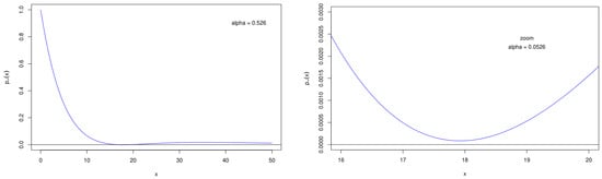
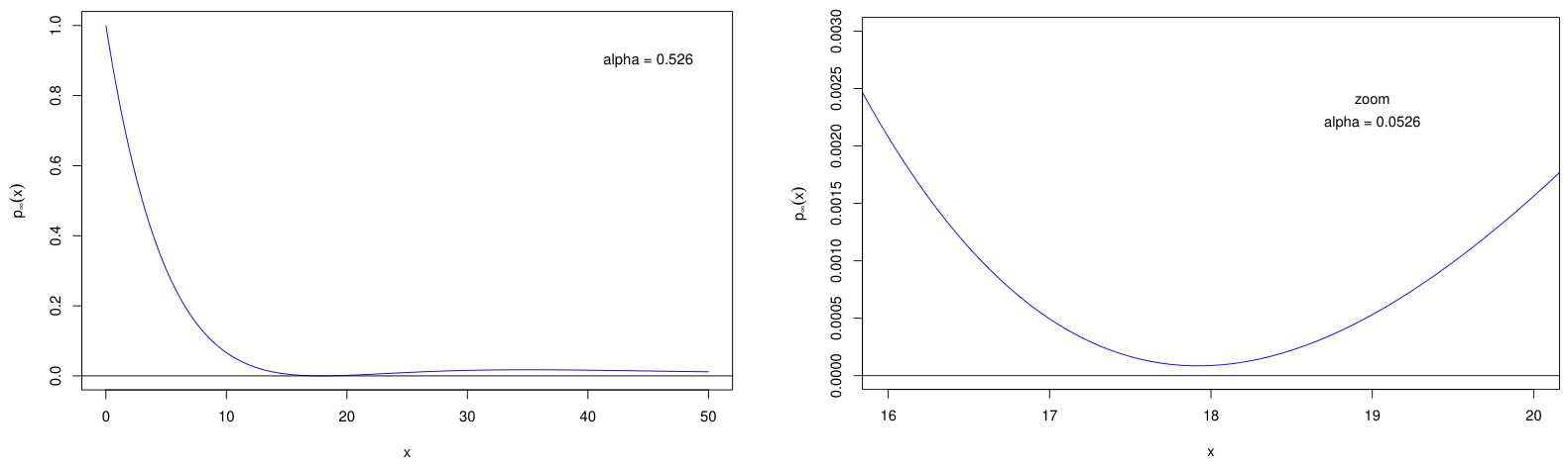
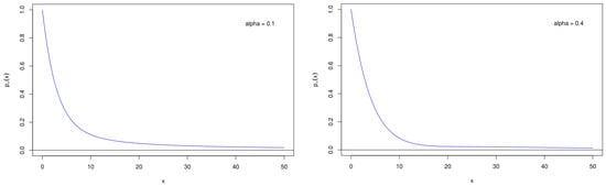
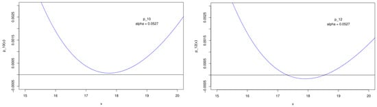
From Table 1, we observe that the condition (20) is fulfilled in each instance. Consequently, it can be inferred that has no roots within the interval . Moreover, we notice that the root increases with the degree m of the odd polynomial . This observation, in conjunction with the graph of presented in Figure 4, provides numerical evidence supporting the conclusion that lacks a positive root when . In fact, for values of less than , the function also appears to be devoid of positive roots, as exemplified by the graphs of in Figure 5, corresponding to and .
Figure 4.
Plot of for as a function of the dimensionless argument x. The right panel shows a zoom near the minimum. Since the curve remains positive and does not cross the horizontal axis, no positive root is detected in this threshold case. Consequently, the fractional model does not predict a critical buckling load at .
Figure 5.
Plots of for and versus the dimensionless argument x. In both cases the function stays above zero over the plotted interval, providing numerical evidence that no positive root exists for these values of . From the mechanical viewpoint, this indicates that the present fractional model does not yield a critical buckling load in this regime.
4.2. Existence of an Even Degree Polynomial with a Positive Root
Now, we will consider . Polynomials , , , and do not have positive roots. However, polynomial does have a positive root, , as shown in Figure 6. Let us set . Then
Figure 6.
Plots of the truncation polynomials and for , shown against the dimensionless argument x. While does not exhibit a positive zero, crosses the horizontal axis near , indicating the appearance of a positive root. This marks the onset of the regime in which the fractional model predicts a critical buckling load.
The Table 2 presents the roots of the polynomials , , and for various values of .
Table 2.
First positive roots of the truncation polynomials , , , and for , , and . For , the closeness of the values , , , and numerically confirms the localization of the first positive root of in a short interval near . For and , the near coincidence of the listed roots shows that the sequence stabilizes rapidly as increases, so that the root of already gives an excellent approximation of the first positive root of .
From this, we observe that . The inequality (21) confirms that Assumption 1 is satisfied. Consequently, based on Theorem 1, it follows that the first positive root of lies within the interval .
Now, let’s assume we aim to find the root of with an error margin less than . To achieve this, it is necessary to ensure that Assumption 2 is fulfilled. Observing the graph of (see Figure 6) we can infer that is decreasing in the interval . Consequently, on , and
thus Assumption 2 is satisfied. Recall that and
which, according to Theorem 2, implies that
Therefore, serves as the desired approximation.
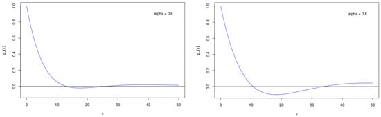
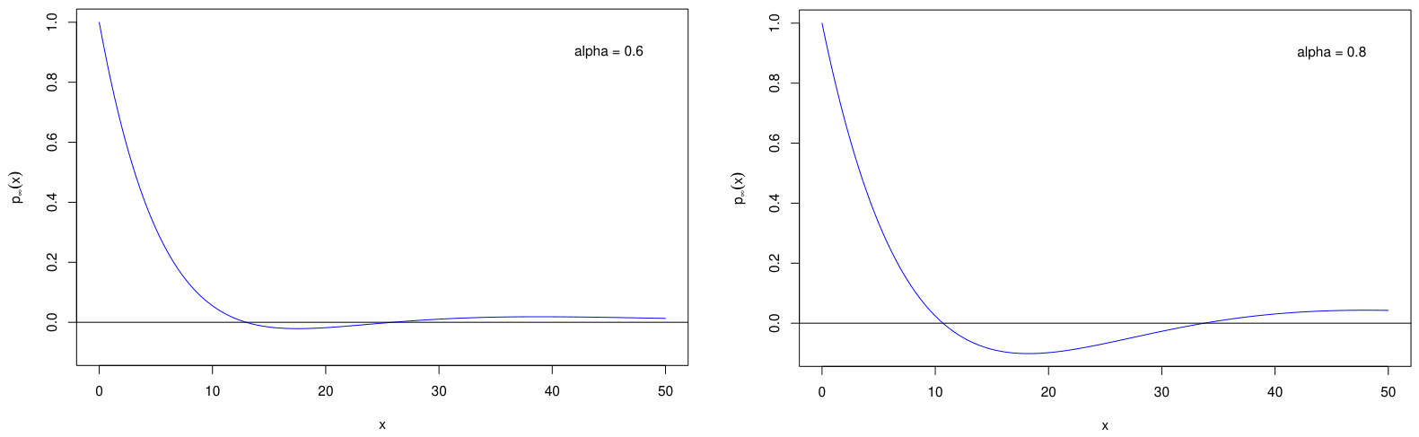
The numerical computations presented in this section indicate that possesses a positive root for the sample values and , whereas no positive root is detected for and . Therefore, within the numerical evidence considered here, the transition between non-existence and existence of a positive root appears to occur near –, see in Figure 7. Additionally, Table 2 illustrates that the root tends to stabilize rapidly with increasing values of . Consequently, the root of serves as an excellent approximation for the root of when is greater than or .
Figure 7.
Plots of for and as functions of the dimensionless argument x. In both cases the curve crosses the horizontal axis, showing that has a positive root for these values of . From the mechanical viewpoint, this implies that the fractional model predicts a critical buckling load in this regime.
To compare the fractional model with the classical Euler theory, it is convenient to introduce the normalized critical load
where denotes the classical Euler critical load corresponding to the case . This dimensionless quantity isolates the contribution of the fractional parameter and makes explicit how the critical load predicted by the model varies with . In particular, the fractional formulation exhibits not only quantitative differences with respect to the classical case, but also a qualitative threshold behavior: for the values discussed in this section, no positive root exists when , and therefore the model does not predict a critical load in that regime.
Table 3 shows that, for the sample values considered here, the ratio increases as decreases. This indicates that the fractional parameter has a strong influence on the buckling threshold within the present formulation, and suggests that may serve as an effective index for distinguishing different buckling responses predicted by the model.
Table 3.
Normalized critical load for selected values of the fractional parameter .
5. Conclusions
In this section, we will address the results obtained. Initially, we have deduced a formula for the radius of curvature that incorporates the fractional index . This formula has been pivotal in formulating our fractional model for column buckling. Subsequently, based on the hypothesis that a polynomial can accurately approximate the elastic curve, we have established the existence of a critical buckling force (Theorem 2). Furthermore, we have managed to calculate an approximation of this critical buckling force that, within a previously defined margin of error (Theorem 3), closely approaches the real force. We observe that for values of , the critical force does not exist, while for , it exists.
A more detailed sensitivity analysis of the transition region near – could provide further insight into the threshold behavior observed in our numerical experiments; however, such an investigation lies beyond the scope of the present work and will be considered in future research.
An important area of opportunity is the exploration of alternative models for beam buckling. This is a vast field, as there are numerous ways in which a beam can buckle (see [17]). Moreover, for each model, different types of fractional derivatives (beyond the Caputo derivative) can be considered, allowing one to physically verify which derivative best captures the buckling behavior.
Expression (1) reveals substantial potential for diversification. By merely altering the curvature moment of the structure of interest, we can derive various fractional differential equations. This observation also suggests a broad range of potential applications. As noted in the Introduction, these curvature-based formulations are relevant to the stability problems arising in civil and aerospace engineering, for example. Although the present work is conceptual, these directions illustrate the practical relevance of the proposed framework and motivate future developments.
It is important to acknowledge several limitations of this study. The first is that the equipment required for the physical validation of the fractional model is very expensive, at least for us. However, other researchers may have access to such equipment or the necessary resources to continue developing our work. The second limitation is theoretical: the initial approximations to are determined by graphically analyzing the roots of the polynomials (see Assumption 1).
Author Contributions
Conceptualization, J.V.-M.; methodology, J.V.-M. and M.R.-A.; formal analysis, J.V.-M. and M.R.-A.; investigation, J.V.-M.; resources, J.V.-M. and M.R.-A.; writing—review and editing, J.V.-M. and M.R.-A.; visualization, J.V.-M. and M.R.-A.; supervision, J.V.-M. All authors have read and agreed to the published version of the manuscript.
Funding
The authors J.V.-M. and M.R.-A. received partial support from grants PIM25-2 and PIM23-6, respectively, from the Universidad Autónoma de Aguascalientes.
Data Availability Statement
This study is purely conceptual and does not utilize specific empirical data.
Acknowledgments
To the referees for their careful review of the manuscript.
Conflicts of Interest
The authors declare no conflicts of interest.
References
- Kumar, S.; Kumar, R.; Agarwal, R.P.; Samet, B. A study of fractional Lotka–Volterra population model using Haar wavelet and Adams–Bashforth–Moulton methods. Math. Methods Appl. Sci. 2020, 43, 5564–5578. [Google Scholar] [CrossRef] [Scilit]
- Hilfer, R. Applications of Fractional Calculus in Physics; World Scientific: Singapore, 2000. [Google Scholar]
- Debnath, L. Recent applications of fractional calculus to science and engineering. Int. J. Math. Math. Sci. 2003, 2003, 3413–3442. [Google Scholar]
- Karniadakis, G.E. (Ed.) Handbook of Fractional Calculus with Applications; Numerical Methods; De Gruyter: Berlin, Germany; Boston, MA, USA, 2019; Volume 3. [Google Scholar]
- Lin, S.-D.; Srivastava, H.M. Some miscellaneous properties and applications of certain operators of fractional calculus. Taiwan. J. Math. 2010, 14, 2469–2495. [Google Scholar] [CrossRef] [Scilit]
- Diethelm, K.; Garrappa, R.; Giusti, A.; Stynes, M. Why fractional derivatives with nonsingular kernels should not be used. Fract. Calc. Appl. Anal. 2020, 23, 610–634. [Google Scholar] [CrossRef] [Scilit]
- Becerra-Guzmán, G.; Villa-Morales, J. Erroneous applications of fractional calculus: The catenary as a prototype. Mathematics 2024, 12, 2148. [Google Scholar] [CrossRef] [Scilit]
- Martínez-Jiménez, L.; Cruz-Duarte, J.M.; Rosales-García, J.J. Fractional solution of the catenary curve. Math. Methods Appl. Sci. 2021, 44, 7969–7978. [Google Scholar]
- Conejero, J.A.; Franceschi, J.; Picó-Marco, E. Fractional vs. ordinary control systems: What does the fractional derivative provide? Mathematics 2022, 10, 2719. [Google Scholar] [CrossRef] [Scilit]
- Ortigueira, M.D. A coherent approach to non-integer order derivatives. Signal Process. 2006, 86, 2505–2515. [Google Scholar] [CrossRef] [Scilit]
- Domokos, G.; Holmes, P.; Royce, B. Constrained Euler buckling. J. Nonlinear Sci. 1997, 7, 281–314. [Google Scholar] [CrossRef]
- Wang, C.M.; Wang, C.Y. Exact Solutions for Buckling of Structural Members; CRC Press: Boca Raton, FL, USA, 2004; Volume 6. [Google Scholar]
- Luo, A.C.J.; Hamidzadeh, H.R. Equilibrium and buckling stability for axially traveling plates. Commun. Nonlinear Sci. Numer. Simul. 2004, 9, 343–360. [Google Scholar] [CrossRef] [Scilit]
- Failla, G.; Zingales, M. Advanced materials modelling via fractional calculus: Challenges and perspectives. Philos. Trans. Ser. A Math. Phys. Eng. Sci. 2020, 378, 20200050. [Google Scholar] [CrossRef] [Scilit] [PubMed]
- Sidhardh, S.; Patnaik, S.; Semperlotti, F. Fractional-order structural stability: Formulation and application to the critical load of nonlocal slender structures. Int. J. Mech. Sci. 2021, 201, 106443. [Google Scholar] [CrossRef] [Scilit]
- Spiegel, M.R. Applied Differential Equations; Pearson: New York, NY, USA, 1980. [Google Scholar]
- Timoshenko, S.P.; Gere, J.M. Theory of Elastic Stability; McGraw-Hill: New York, NY, USA, 1961. [Google Scholar]
- Ortigueira, M.; Machado, J. Which derivative? Fractal Fract. 2017, 1, 3. [Google Scholar] [CrossRef] [Scilit]
- Diethelm, K. The Analysis of Fractional Differential Equations; Lecture Notes in Mathematics; Springer: Berlin/Heidelberg, Germany, 2010; Volume 2004. [Google Scholar]
- Kilbas, A.A.; Srivastava, H.M.; Trujillo, J.J. Theory and Applications of Fractional Differential Equations; North-Holland Mathematics Studies; Elsevier: Amsterdam, The Netherlands, 2006; Volume 204. [Google Scholar]
- Samko, S.G.; Kilbas, A.A.; Marichev, O.I. Fractional Integrals and Derivatives: Theory and Applications; Gordon and Breach Science Publishers: Yverdon, Switzerland, 1993. [Google Scholar]

Disclaimer/Publisher’s Note: The statements, opinions and data contained in all publications are solely those of the individual author(s) and contributor(s) and not of MDPI and/or the editor(s). MDPI and/or the editor(s) disclaim responsibility for any injury to people or property resulting from any ideas, methods, instructions or products referred to in the content. |
© 2026 by the authors. Licensee MDPI, Basel, Switzerland. This article is an open access article distributed under the terms and conditions of the Creative Commons Attribution (CC BY) license.