


Abstract
The evaluation of optimization algorithms for electric vehicle routing problems depends strongly on the quality of the benchmark instances used during experimentation. However, many synthetic instances simplify the joint effects of geometry, topography, operation, and energy, which can distort algorithmic assessment. This article proposes a modular and reproducible pipeline for generating synthetic instances of the Electric Vehicle Steiner Traveling Salesman Problem (EV-STSP), calibrated from a real urban reference network based on publicly available Madrid data. The pipeline combines directed graph construction, geometric control, attribute enrichment, charging-infrastructure placement, structured export, and explicit traceability mechanisms. To assess the realism of the generated instances, a three-level validation protocol is introduced, covering marginal distributional similarity, physical coherence among dependent variables, and structural–operational consistency. A controlled ablation design is then used to quantify the contribution of individual modules to overall benchmark realism. Within the experimental domain explored here, the results show that benchmark realism is not supported uniformly by all modules; instead, it depends primarily on arc-length generation, topographic alignment, and energy modeling. The proposed framework therefore offers not only a reproducible way to generate EV-STSP benchmarks, but also an explicit methodology for verifying whether such benchmarks are suitable for comparative algorithmic experimentation.
1. Introduction
In recent years, transport electrification has become a major research topic in logistics and optimization. Within this context, routing problems for electric vehicles have expanded rapidly, both in the number of problem variants considered and in the diversity of solution approaches, driven by the need to reduce emissions, improve energy efficiency, and adapt route planning to new operational constraints. Recent surveys show that the Electric Vehicle Routing Problem (EVRP) has become a well-established research domain, with multiple problem classes, algorithms, and benchmark sets, while also warning that a substantial portion of the literature still oversimplifies real operating conditions or remains only partially connected to the actual capabilities of vehicles and their urban environment [1,2,3].
Among the most influential variants is the Electric Vehicle Routing Problem with Time Windows (E-VRPTW), introduced to explicitly represent the limited driving range of vehicles, the need for en-route charging, and essential operational constraints such as capacity and time windows [4]. Building on this model, the literature has shown that the problem does not depend only on deciding which customers to visit and in what sequence, but also on when to recharge, where to do so, and under which recharging policy. In this line of work, it has been shown that allowing partial recharges can modify route structure and improve decision quality [5], whereas full battery swapping can substantially reduce station service time, albeit at the cost of additional infrastructure and operational assumptions [6]. Taken together, these studies show that the representation of the recharging process is not an accessory detail, but rather a structural part of the problem.
In parallel, the literature has incorporated progressively more realistic energy models. In particular, it has been argued that the energy consumption of an electric vehicle should not be treated solely as a linear function of traveled distance, since variables such as speed, road gradient, and carried load substantially modify the energy consumed and, consequently, route feasibility. More specifically, it has been documented that realistic energy consumption depends on variables such as speed, gradient, and payload, because these factors directly affect the available driving range and the timing of recharging decisions [7]. Consistently, richer formulations have explicitly incorporated speed and payload within the energy model [8]. More recently, in time-dependent urban settings, it has been observed that speed variations affect not only travel times but also battery depletion, and that ignoring this dependency may induce operational infeasibilities [9].
Beyond energy enrichment, the literature has also begun to model more complex operational structures. For example, piecewise charging schemes and stations with limited charger capacity introduce an explicit interaction between routing and scheduling decisions [10]. This evolution confirms that contemporary EV routing can no longer be understood merely as a green extension of the classical VRP, but rather as a family of problems in which physical, temporal, and infrastructural constraints interact closely. Nevertheless, this same progress makes a methodological tension more visible: although the literature has advanced considerably in the formulation and solution of increasingly rich EVRP variants, it is still necessary to strengthen the experimental basis on which algorithms are compared, especially when their behavior is to be assessed in urban settings that are sensitive to energy consumption. In that sense, operational realism is no longer a marginal refinement of EVRP modeling, but a necessary condition for correctly interpreting the performance of solution methods [3,7,8,9,10].
In this study, that need is addressed through a real reference case based on a directed urban road network from Madrid, enriched with geometric, topographic, and operational information for the study of the Steiner Traveling Salesman Problem in the context of electric vehicles [11]. This case was selected because three key data layers (urban network, elevation, and traffic) are publicly available and reproducible as supplementary material accompanying the original study. To ensure traceability, version 1.1 of the Zenodo repository is used, which includes both the reference data and the energy model employed in that work [12]. The input materials are organized into three main layers: a road layer represented by a directed urban graph; a topographic layer that associates elevation with the network and allows relationships among gradient, elevation, and geometry to be derived; and an operational layer composed of hourly traffic snapshots for October and November 2022, used to obtain representative speeds by segment. In addition, the energy_estimation_full.h5 model and its associated scaler, scaler_full.pkl, are integrated as inherited reference components for estimating arc-level energy consumption under a consistent input scheme. This empirical basis not only contributes realism, but also makes it possible to assess whether a preexisting energy model remains coherent when applied to synthetically generated attributes.
A parallel, though considerably smaller, line of research has focused specifically on generating benchmark instances for electric vehicle routing problems. In this context, Schneider et al. [4] introduced the E-VRPTW benchmark set that became the de facto standard for algorithmic comparison, constructed from modified Solomon instances with synthetic locations and no distributional calibration. Hiermann et al. [13] extended this approach to heterogeneous fleets and incorporated basic operational checks on recharging station usage, but without distributional validation and with a constant energy consumption model that does not depend on the carried load. Along similar lines, Montoya et al. [14] generated instances with nonlinear recharging functions from real vehicle data, but placed nodes in a synthetic 120 × 120 km2 space without topographic calibration; the authors themselves acknowledge that energy consumption was simplified as the vehicle consumption rate multiplied by the arc distance, omitting the effect of gradient, speed, and load. Froger et al. [15], Schiffer and Walther [16], and Felipe et al. [17] also contributed instances or benchmark extensions for various EVRP variants, but none incorporated distributional validation or explicit physical coherence mechanisms among the generated attributes. In the classical VRP domain, Uchoa et al. [18] established a methodological reference by controlling the geometric distribution of nodes, but without the physical and energy attribute layer that electric routing requires. In the Steiner TSP domain more specifically, Rodríguez-Pereira et al. [19] proposed compact ILP formulations and exact branch-and-cut algorithms for the undirected STSP, validating them on instances from the literature but without a calibrated synthetic generator or distributional validation; and Agarwal et al. [20] addressed a bi-criterion variant with time windows for last-mile electric vehicle logistics on real Amazon delivery routes, incorporating gradient-aware energy consumption, but similarly without a formal benchmark generation protocol or physical-coherence verification. Taken together, the review of these works reveals three systematic gaps: none applies formal distributional tests to verify that synthetic instances reproduce the distributions of a real urban network; physical coherence among dependent variables (length, gradient, speed, and energy) is rarely verified explicitly; and module-level ablation analysis to identify which generator components are critical for benchmark realism is absent from the reviewed literature. Table 1 synthesizes these methodological dimensions across the reviewed works and positions the present study with respect to each identified gap.
Table 1.
Methodological comparison of related works for EV-routing and Steiner TSP benchmark generation.
Against this background, the article proposes a modular and reproducible pipeline for generating EV-STSP synthetic instances calibrated from a real urban reference network. The contribution goes beyond producing new instances: it establishes an explicit procedure for evaluating whether those instances preserve properties that matter for algorithmic experimentation. To this end, the pipeline integrates modules for structural construction and for geometric, topographic, operational, and energy enrichment, and is paired with a three-level validation protocol, a module-wise ablation design, and a configuration synthesis for generating more defensible benchmarks. From this perspective, the main contribution of the study is to show, within the experimental domain examined here, that the validity of a synthetic EV-STSP benchmark depends on simultaneously preserving distributional similarity, physical coherence, and operational consistency, and that these properties are driven by a critical subset of generator modules rather than by all of them equally. Accordingly, the article does not propose a new solver for a richer EVRP variant; instead, it provides a reproducible and auditable experimental basis for the methodologically sound comparison of algorithms on EV-STSP. While individual elements such as distributional calibration, multi-level validation, and ablation analysis are known in adjacent methodological domains, their joint application to EV-STSP benchmark generation, where physical coherence among arc length, gradient, and energy is an operational constraint rather than a decorative property, constitutes a contribution that goes beyond integration: it proposes an auditable framework for verifying whether a synthetic instance is fit for algorithmic experimentation, a design requirement not addressed by any of the reviewed benchmark generators for EV-STSP. In view of these gaps, the novelty of the present contribution rests on three aspects that, taken together, have not been addressed in an integrated manner in the reviewed works: (i) distributional calibration of the instance generator from a real urban network with publicly available and traceable data, which distinguishes the approach from generators based on uncalibrated synthetic distributions; (ii) a validation protocol structured at three levels (distributional similarity, physical coherence among dependent variables, and structural–operational consistency) that allows benchmark quality to be audited rather than assumed; and (iii) a module-level controlled ablation design that quantifies the individual contribution of each pipeline component to experimental realism, an analysis that does not appear systematically in any of the reviewed benchmark generators for EV-STSP or its closest variants.
2. Materials and Methods
This section presents a reproducible methodology for generating realistic synthetic instances of the Electric Vehicle Steiner Traveling Salesman Problem (EV-STSP) from a reference urban network. The main contribution is methodological: a modular pipeline is introduced that constructs a directed road network enriched with geometric, topographic, operational, and energy attributes and then transforms it into parameterized instances ready for experimentation. From an optimization standpoint, the purpose of the pipeline is to produce benchmark instances whose statistical and physical–operational structure does not distort the comparative evaluation of algorithms for EV-STSP.
The pipeline is calibrated with real data and validated through three complementary levels: distributional similarity of key attributes, coherence among physically related variables, and structural and operational checks on the generated network. In addition, the process incorporates explicit logging of parameters, random seeds, and metadata in order to ensure traceability, reproducibility, and fair comparison across experimental configurations. Figure 1 summarizes the general methodological workflow.
Figure 1.
Overview of the pipeline for generating EV-STSP instances.
Figure 1 synthesizes the overall sequence of the pipeline, from the selection of the real reference case and the calibration of attributes to the generation, validation, and export of EV-STSP instances. This organization makes it possible to clearly distinguish the stages of structural construction, progressive enrichment, infrastructure incorporation, and quantitative evaluation. Based on this general view, the section is organized as follows: the optimization problem that motivates instance generation is first formally defined; the real reference case and calibration materials are then presented; and the construction, enrichment, validation, and export stages of the pipeline are subsequently developed.
To clearly delimit the properties that the pipeline must preserve from the outset, it is first necessary to formally establish the formulation of the optimization problem for which these instances are intended. The formal definition of the EV-STSP makes it possible to specify which structural elements (network topology, arc-level energy attributes, required nodes, and support infrastructure) must be present and internally coherent in an instance for it to be useful in the experimental evaluation of algorithms.
2.1. Problem Statement
The EV-STSP is a combinatorial optimization problem defined over a directed graph , where V is the set of nodes representing road intersections and A is the set of arcs representing oriented road segments. Each arc carries a vector of physical–operational attributes: length , gradient , elevation change , representative speed , travel time , and energy consumption . The nodes are classified into four categories: the depot d, the required nodes that must be visited, the battery swap stations , and the remaining ordinary nodes.
The objective is to determine a route that departs from the depot, visits all required nodes, and returns to the depot, simultaneously minimizing four criteria: total distance traveled (), total energy consumption (), number of battery swaps performed (), and total route time including swap service times (). The solution is represented by three families of binary variables indexed by position : (whether arc is traversed at position t), (whether the vehicle occupies node i at position t), and (whether a battery swap is performed at station s at position t).
The model is subject to flow and position-uniqueness constraints on the graph, mandatory coverage of all required nodes, energy feasibility (the battery charge must satisfy at all times), and limits on the number and frequency of swaps permitted per station. This structure combines the topological richness of the Steiner Traveling Salesman Problem with the energy and infrastructure constraints of electric vehicle routing, which imposes specific demands on the quality of the benchmark instances used for experimental evaluation. A complete mathematical formulation of the model is provided in [11].
2.2. Real Case and Input Materials (Madrid)
The real reference case corresponds to a directed urban road network from Madrid, enriched with geometric, topographic, and operational information for the study of the Steiner Traveling Salesman Problem in the context of electric vehicles [11]. This case was selected because of the public and reproducible availability of three key information layers, namely, urban network, elevation, and traffic, published by the authors as supplementary material. To ensure traceability, this work uses version 1.1 of the Zenodo repository, which includes both the reference data and the energy model employed in the original study [12].
The input materials are organized into three main layers. The first corresponds to the road layer, represented by a directed urban graph in which nodes model intersections and arcs represent oriented segments in accordance with traffic direction. The second corresponds to the topographic layer, which allows elevation to be associated with the network and, from that basis, the effect of gradient on energy-related magnitudes to be analyzed. The third is the operational layer, composed of traffic measurements in the form of hourly snapshots for the months of October and November 2022, used to obtain representative speeds by segment.
From these inputs, this work constructs an empirical calibration set at the arc level, from which samples of key variables such as length, gradient, and speed are extracted. In particular, the traffic measurements are used to characterize the operational behavior of the network, while the topographic artifacts make it possible to derive and verify relationships among gradient, elevation, and geometry. In addition, the energy_estimation_full.h5 model, together with its associated scaler scaler_full.pkl, is integrated as a reference component inherited from the Madrid case to estimate arc-level energy consumption under a consistent input scheme. This choice allows the study to examine whether a preexisting energy model remains coherent when operating on attributes generated by the proposed synthetic pipeline, an aspect that is explicitly evaluated in the later validation and ablation stages.
Table 2 summarizes the files used and their role within the methodological process.
Table 2.
Materials of the Madrid case and their use in this study.
Based on these materials, the methodology defines a common empirical reference not only to calibrate the pipeline modules, but also to audit whether the generated instances preserve properties that are relevant to the evaluation of optimization algorithms in electrified urban networks. The following subsection describes the overall view of the proposed pipeline and how these inputs are transformed into generation rules, calibration parameters, and quantitative checks that produce reproducible EV-STSP instances.
In addition to the data artifacts, reproducibility also depends on the execution environment and on the implementation of the pipeline. The reported campaign was implemented in Python 3.11.9, using NumPy and Pandas for data handling, NetworkX for graph construction, SciPy for KDE, distance calculations, and LSQR solving, joblib for loading serialized artifacts, and tqdm for run monitoring. The ANN energy module is invoked through a prediction wrapper when available; if the predictor is unavailable or returns invalid outputs, the workflow falls back explicitly to a robust empirical-median baseline and records both the requested energy mode and the mode ultimately used.
2.3. Overview of the Proposed Pipeline
Several paradigms have been proposed for generating benchmark instances for combinatorial optimization problems, each responding to a different generation objective. One influential line adopts evolutionary or diversity-driven search: Bossek and Neumann [21] used a quality-diversity (QD) approach based on Map-Elites to generate sets of TSP instances whose features differentiate the performance of competing solvers, covering a wide region of the instance feature space in a single evolutionary run; Marrero [22] developed a framework based on novelty search (DIGNEA) that produces diverse instances capable of discriminating among a portfolio of algorithms across several optimization domains. A second line uses deterministic or structural construction: Liang et al. [23] proposed a procedure that builds small TSP instances with a controlled number of local optima and a known range of objective values, enabling targeted analysis of algorithm sensitivity to structural instance properties. While these approaches represent important methodological advances for algorithm characterization, they share a common scope that differs substantially from the present work: they operate on abstract combinatorial instances (typically classical TSP on unconstrained Euclidean point sets) and do not calibrate the instance generator from empirical measurements of a real urban network. Physical coherence among geometrically and operationally correlated attributes (arc length, gradient, speed, and energy) is not a design requirement in these approaches, since the problems addressed do not exhibit this type of physical dependency. The pipeline proposed here addresses a qualitatively different generation objective: to produce instances of the EV-STSP (a directed, multi-attribute, energy-constrained variant of the STSP) whose attribute distributions and physical interrelationships reflect those of a real urban road network, so that the resulting benchmarks are operationally defensible for the comparative evaluation of EV routing algorithms.
The proposed methodology is organized as a modular pipeline for generating synthetic EV-STSP instances from a real reference case. Its structure separates base-network construction, progressive attribute enrichment, infrastructure incorporation, and quantitative validation, while maintaining explicit dependencies among modules and avoiding rigid assumptions when the empirical evidence suggests nonlinear behavior.
In a first stage, the pipeline constructs a directed base graph of controlled size, which acts as the initial topological support for the synthetic instance. On this basis, an initial spatial geometry is defined through the assignment of coordinates and, when appropriate, the geometric scale is adjusted to maintain coherence between the spatial representation and the metric later induced by arc attributes.
Subsequently, the network is enriched sequentially with geometric, topographic, operational, and energy attributes. First, arc lengths are assigned, fixing the metric scale of the network. Next, gradients are incorporated and consistent nodal elevations are reconstructed. Then, arc speeds are assigned to represent operating conditions comparable to the real reference. Finally, arc-level energy consumption is estimated using the energy model integrated into the pipeline.
Once the network has been enriched, the pipeline incorporates charging stations through a coverage criterion defined over the underlying physical network. The resulting instance is exported in a structured format that integrates the directed network, the charging infrastructure, and the global configuration of the problem. In parallel, parameters, seeds, and metadata are logged, and a quantitative validation protocol is applied to compare the synthetic instance against the real reference case.
Unlike approaches that generate attributes in isolation, the proposed pipeline maintains explicit dependencies among modules in order to avoid instances that appear plausible in marginal variables but are incoherent from a physical or operational perspective. This property is particularly relevant when the instances are to be used as benchmarks for comparing optimization algorithms.
2.4. Construction of the Directed Base Graph and Geometric Control
The generation of synthetic instances begins with a directed base graph of controlled size, conceived as the structural scaffold on which the enrichment modules are later applied. This graph is built as a directed grid of nodes, where each node represents an abstract intersection and each arc represents an oriented road segment. Throughout this work, a directed arc is denoted by the ordered pair , where u is the origin node and v is the destination node; the arc is distinct from and implies a one-way traversal from u to v. The purpose of this stage is to define a stable and parameterizable directed topology that allows, in a consistent manner, the effects introduced by the later modules of the pipeline.
To facilitate reproducibility, the construction flow of the base graph is summarized in Algorithm 1, which integrates directed-grid generation, optional strong-connectivity control, and initial geometric assignment.
| Algorithm 1 Generation of the directed base graph and geometric control |
|
Input: rows r, columns c, spatial box B, flags strong (enforce strong connectivity), autoScale (automatic scale alignment). Output: directed graph G with node coordinates. 1. Create node set and initialize . 2. For each node, add horizontal and vertical arcs according to a periodic directionality pattern (period 3: horizontal links use , vertical links use ). 3. Form the directed graph . if strong = true and G is not strongly connected then 4. Connect representatives of strongly connected components with minimal arcs. end if 5. Assign coordinates to each node through regular interpolation inside B. if autoScale = true then 6. Adjust B with a bounded factor to align the scale and reassign coordinates. end if 7. Return G. |
At the structural level, the grid is generated by connecting each node to its immediate neighbors and assigning directions through a systematic pattern that introduces traffic directions without turning the network into a fully bidirectional graph. This design preserves geometric regularity and introduces controlled directionality, a desirable condition for abstractly representing circulation constraints present in real urban networks.
When the experimental design requires it, a strong-connectivity mechanism is activated to ensure global reachability in the directed graph. In that case, the strongly connected components are identified and their representative nodes are connected in a simple cycle, adding an arc between consecutive representatives whenever it does not already exist. This mechanism restores global reachability with minimal perturbation of the original density.
Finally, the base graph is assigned a spatial geometry through coordinates regularly distributed within a spatial box. Optionally, this geometry is automatically rescaled using the ratio between the median simulated length and the median geodesic distance induced by the initial spatial box; the resulting factor is multiplied by bbox_scale and bounded by the reference bounding box.
The choice of a regular grid as the base topology is a deliberate design decision that prioritizes reproducibility and controllability of the ablation experiment: since the topology is fully deterministic as a function of r and c, its effect on instance attributes can be isolated from the variations introduced by the calibration modules. However, this choice implies limitations that must be explicitly acknowledged. Real urban road networks exhibit heterogeneous degree distributions, spatial irregularities, and connectivity asymmetries that are not captured by a uniform grid. In particular, a regular grid overestimates the topological regularity of real networks, underestimates the presence of dead ends or low-connectivity branches, and does not reproduce the non-uniform spatial distribution of intersections in dense urban environments. From the perspective of the EV-STSP, these differences may affect the distribution of shortest-path lengths between required nodes and the efficiency of swap station coverage. However, since the arc attributes (length, gradient, and energy consumption) are calibrated from the Madrid reference network, the pipeline preserves the distribution of operationally relevant attributes regardless of the grid topology. Extending the pipeline to topologies based on real networks or stochastically generated graphs constitutes a natural direction for future work.
2.5. Attribute Enrichment on Arcs and Nodes
Once the directed base graph has been constructed and its initial geometry defined, the methodology proceeds to the progressive enrichment of attributes on arcs and nodes, to transform an abstract topology into a synthetic network that is operationally interpretable and comparable to the real reference case. This stage constitutes the functional core of the pipeline, as it incorporates the variables that determine the metric, topography, road operation, and energy consumption of the generated network.
Enrichment is organized sequentially, following physical dependencies among variables. First, arc lengths are assigned, because they fix the metric scale of the network. Next, gradients are incorporated and consistent nodal elevations are reconstructed. Then, arc speeds are assigned to represent operating conditions comparable to the real reference. Finally, arc-level energy consumption is estimated by jointly integrating the geometric, topographic, and operational information relevant to the electric-vehicle context.
To preserve consistency with the Madrid case, each enrichment module is calibrated using the empirical set described in Section 2.1. Rather than imposing rigid parametric assumptions, the methodology prioritizes data-driven strategies and minimal plausibility controls in order to reproduce observed distributions and avoid degenerate or physically inconsistent configurations.
2.5.1. Generation of Arc Lengths
The first variable incorporated into the synthetic graph is arc length, since it fixes the metric scale on which gradient, speed, and, ultimately, energy consumption are later interpreted. In this methodology, lengths are assigned in a data-driven manner, using as reference the empirical sample extracted from the real Madrid case described in Section 2.1, with the objective of reproducing its variability without imposing rigid parametric assumptions.
Let E be the set of arcs of the base graph, with . From the collection of lengths observed in Madrid, expressed in meters, an empirical reference distribution is defined from which N synthetic values are generated, one for each arc . In practice, the methodology contemplates two alternative generation mechanisms, selected according to the experimental design.
The first mechanism consists of empirical quantile-based sampling. In this case, the quantile function of the real sample is constructed and N quantile levels are selected with controlled randomness. Each level is transformed into a synthetic length through interpolation over the observed empirical distribution.
The second mechanism consists of sampling based on nonparametric density estimation by means of KDE [24]. In this case, a smoothed density is fitted over the real lengths and N samples are generated from that estimate. To maintain metric plausibility, the generated lengths are restricted through robust quantiles of the empirical support and a strictly positive lower bound is imposed. In the implementation, the generation support is bounded by robust quantiles of the empirical sample in order to avoid artificial tails or values incompatible with the urban scale of the reference.
Regardless of the sampling mechanism used, the result of this stage is the set of arc lengths associated with the arcs of the base graph. These lengths establish a network with an interpretable metric that is statistically consistent with the reference. In the current implementation, when KDE is used, the real sample is first trimmed between quantiles 0.001 and 0.999, simulated lengths are forced to be strictly positive (minimum 1 m), then bounded to the empirical interval , and 2% of the arcs are reassigned within to preserve plausible short segments without introducing artificial tails.
2.5.2. Generation of Arc Gradients and Topographic Alignment
Once the metric of the network has been defined through arc lengths, the topographic component is incorporated by assigning a gradient to each arc. This attribute is relevant in the context of electric vehicles because it influences resistance to motion and, consequently, energy consumption. The objective of this stage is to generate slopes that are comparable with the real reference case and, at the same time, compatible with the already established metric scale.
From the Madrid case described in Section 2.1, an empirical sample of arc gradients is obtained to serve as the calibration basis. Let be the gradient associated with arc , understood as a dimensionless ratio between elevation change and length. The assignment of gradients in the synthetic network is performed by introducing a minimal coupling with arc length, so that the combination produces plausible altimetric variations and avoids physically unrealistic configurations. This local relationship is summarized in Equation (1).
where denotes the signed elevation change along arc e, with and being the elevation at the origin and destination node of arc e, respectively.
As a coherence control, the induced altimetric magnitude is evaluated for each arc and, whenever it systematically departs from the empirical reference support, the corresponding gradient is corrected through resampling or controlled truncation within plausible bounds. In the base campaign, gradients were generated with a length-conditioned k-NN scheme [25], parameterized as follows: nearest neighbours in arc-length space, inverse-distance weighting with exponent power , and Gaussian perturbation with standard deviation jitter (expressed as a fraction of the empirical gradient range) to prevent exact replication of reference values. Gradients were then aligned by length deciles to preserve the empirical length–slope dependence; variant V4 replaces this logic with marginal KDE sampling [24].
2.5.3. Reconstruction of Nodal Elevations from Gradients
Once arc gradients have been assigned, a nodal elevation profile that is consistent with this topographic information is reconstructed. This step makes it possible to endow the synthetic network with an interpretable topography at the node level while, at the same time, preserving internal coherence between arc slopes and the altimetric differences of their endpoints.
Let be the directed graph enriched with lengths and gradients . For each arc , the induced altimetric difference is approximated as in Equation (1). Based on these relationships, nodal elevations are estimated through a global least-squares adjustment given by Equation (2):
Because this formulation is invariant under global additive translations, a reference node is fixed with , which makes it possible to obtain a unique solution for the reconstructed elevation profile.
This formulation makes it possible to obtain a globally consistent topography without depending on a single propagation path through the network, which is particularly important in directed graphs with multiple cycles and alternative routes. In this way, the procedure reduces the accumulation of local inconsistencies and avoids incompatible assignments for the same node.
The global least-squares formulation is the appropriate choice precisely for networks with cycles. Spanning-tree-based propagation approaches assign elevations by following a single path from a root node, which causes local inconsistencies to accumulate along each propagation path and produces node elevation estimates that depend on the chosen spanning tree, which is an undesirable property in a reproducible pipeline. By contrast, the least-squares adjustment distributes residual errors optimally across all arcs simultaneously, minimizing the global inconsistency between the assigned gradients and the resulting elevation differences, regardless of the cyclic structure of the graph. Regarding the impact of elevation reconstruction errors on downstream energy estimation, the metric included in the validation protocol (Section 2.7) serves as an empirical proxy: it quantifies the degree to which the relationship between energy and altimetric change is preserved in the synthetic instance relative to the real reference. The consistently low values of observed across scenarios V0–V6 (reported in Table 6) indicate that elevation reconstruction errors do not materially distort the energy–elevation relationship in practice. Formal error bounds on the least-squares residuals are not derived here and are identified as a direction for future work.
As a final verification, the relationship given in Equation (3) is checked locally on representative arcs, correcting only systematic deviations when they depart from the empirical reference support. The result of this stage is a synthetic network with nodal elevations and arc-level altimetric differences that are mutually compatible and ready for the incorporation of operational and energy attributes.
2.5.4. Assignment of Arc Speeds and Operational Consistency
Once the metric of the network has been defined through arc lengths and topographic reconstruction has been completed from gradients and nodal elevations, the operational dimension is incorporated by assigning a speed to each arc. This attribute is relevant because it represents the circulation regime of the network and constitutes a necessary input for estimating energy consumption.
From the operational information available for Madrid, particularly the hourly traffic snapshots, an empirical sample of segment speeds is obtained together with its temporal variability. Let be the speed associated with arc . Synthetic generation assigns to each arc a representative speed through a data-driven scheme calibrated from that empirical sample.
In the experimental campaign reported in this manuscript, the assignment of speeds remained in empirical mode in all ablation scenarios. Consequently, speed acted as a controlled component of the pipeline and not as a discriminating dimension in the comparison among variants. Nevertheless, its incorporation remains necessary within the methodological workflow.
As an operational-consistency control, it is verified that the assigned speeds produce arc travel times that are compatible with the support observed in the real case. In particular, for each arc the travel time is defined as in Equation (4).
The resulting values are then checked to ensure that they remain within an interpretable regime for segment length and the reference urban conditions.
Accordingly, within the experimental batch reported here, speed is interpreted as a control variable and not as an ablated factor, which makes it possible to attribute the observed differences more clearly to the geometric, topographic, and energy modules.
2.5.5. Arc-Level Energy Consumption Estimation Through the Model Integrated into the Pipeline
With the synthetic network already enriched in its geometric, topographic, and operational components, the next step consists of estimating arc-level energy consumption. This stage is especially relevant in the context of electric vehicles because it transforms physical and operational network attributes into a magnitude directly related to route feasibility under battery constraints. In the proposed methodology, energy estimation is implemented, in its reference variant, through the model energy_estimation_full.h5 inherited from the Madrid case.
The incorporation of this model makes it possible to examine whether a preexisting energy estimator remains coherent when operating on attributes generated by the synthetic pipeline. Consequently, within this work the energy module is not assumed to be valid by construction, but rather treated as a component integrated into the methodological workflow whose consistency is evaluated later through the validation protocol and the ablation design.
In the reported implementation, energy estimation supports three modes: ann, linear, and median. In ann mode, the script delegates prediction to a wrapper of the inherited neural network. This routine receives as inputs the origin and destination nodes of the arc, the temporal context of the estimation, and the graph enriched with nodal attributes such as position, elevation, speed, and road type. In the main campaign, this context was fixed with workingday = 1, weekday = Tuesday, and hour = 12. In the linear baseline, arc energy is approximated by Equation (5). This formulation is a piecewise linear regression that explicitly separates the contribution of uphill segments (, positive elevation gain) from downhill segments (, negative elevation gain), since their physical effect on energy consumption is asymmetric: climbing increases traction demand whereas descending may partially recover energy through regenerative braking. The two terms act as hinge functions that assign independent coefficients to each regime, which distinguishes this model from a standard ordinary least squares regression over a single elevation-change predictor.
When energy_mode = linear is selected, the coefficients are fitted by least squares on the real case using an intercept, length, and elevation gains/losses; when energy_mode = median is selected, each arc receives the empirical median energy. If the ANN predictor is unavailable or returns invalid values, the workflow explicitly degrades to the median baseline and records in metadata both the requested energy mode and the one ultimately used. In the reported scenarios, V0–V6 operate with energy_mode_used = ann, V7 with linear, and V8 with median. As a minimal consistency control, all predictions are contrasted against the observed empirical support and preserved in logs for later analysis.
2.6. Placement of Charging Stations Through Coverage over the Network
Once the synthetic network has been enriched with geometric, topographic, operational, and energy attributes, the methodology incorporates charging infrastructure by selecting a subset of nodes as stations. This stage seeks to ensure spatial accessibility to the infrastructure within the generated network.
Station placement is formulated as a coverage problem over the underlying physical network, parameterized by a radius , which represents the maximum acceptable distance between a node and its nearest charging station. Although the final instance is directed, coverage is evaluated on an undirected representation of the network, because at this stage the goal is to model accessibility to the infrastructure.
Let be the undirected physical network, weighted by length, and let be the shortest-path distance between nodes u and v on . For each candidate node , its coverage set is defined as in Equation (6).
The objective is to select a set of stations such that every node is covered by at least one station, that is,
To construct this solution, the methodology adopts a greedy coverage strategy [26]. At each iteration, the node that covers the largest number of still-uncovered nodes within radius is selected as a station, and the process is repeated until full network coverage is reached. In the current implementation, the code does not impose an additional lexicographic tie-break, so ties are resolved according to the iteration order of the candidate-node container; because this behavior was not used as an experimental factor, coverage is interpreted here as a feasible benchmark construction rather than as an exact solution of the coverage problem. The result of this stage is a set of nodes labeled as charging stations, together with the value of the coverage radius employed.
2.7. Instance Export and EV-STSP Parameterization
Once the enriched network and the charging infrastructure have been defined, the next step consists of materializing an experimental instance in a structured format that can be directly used by optimization algorithms. This stage transforms the generated network into a set of files that integrates structure, operational attributes, charging infrastructure, and global problem parameters.
Export is performed at two complementary levels. At a first level, the pipeline stores a direct representation of the generated network in a run-specific folder identified by a variant label and a unique execution identifier. This output records a main file containing the directed network arcs, a file listing the nodes selected as charging stations, and a metadata file in JSON format that documents the instance generation configuration. This organization makes it possible to isolate each execution experimentally and avoid overwriting across runs.
The main file of the directed network contains, for each arc , the attributes required for later analysis, including length, elevation at the origin node, elevation at the destination node, gradient, speed, and estimated energy. Complementarily, the station file stores the subset of nodes labeled as charging points. Taken together, these artifacts constitute the immediate output of the pipeline before its transformation into the final problem instance.
At a second level, the pipeline processes this intermediate output to construct a structured EV-STSP instance under a full battery-swapping scheme. This transformation generates the files evstsp_swap_edges.csv, evstsp_swap_nodes.csv, evstsp_swa p_stations.csv, evstsp_swap_config.csv, and evstsp_swap_README.txt. In this processed version, the directed network preserves the basic arc attributes and adds derived quantities useful for experimentation, particularly travel time and estimated power by arc. In particular, arc travel time is calculated according to Equation (8).
The exported parameterization explicitly distinguishes among ordinary nodes, required nodes, station nodes, and the depot node. To this end, the node file incorporates binary indicators that make it possible to identify whether a node belongs to the charging infrastructure, whether it is part of the subset of required nodes, and whether it acts as the depot. In this way, the final instance is ready to represent an experimental EV-STSP variant in which not all nodes of the network must necessarily be visited.
Battery-swapping infrastructure is also exported explicitly. For each station node, operational parameters such as swap time, available pack inventory, and the energy associated with each pack are recorded. At the global level, the configuration file incorporates total battery capacity, initial state of charge, minimum allowed level, swapping mode, maximum number of swaps, the speed limit considered, and the identifier of the depot. In methodological terms, this stage provides a structured and reusable representation of the generated instance, integrating the network, infrastructure, and global problem parameters in a format usable directly by optimization algorithms. The aspects associated with detailed logging of configuration, metadata, and validation results are described in Section 2.8. This structured representation turns the output of the pipeline into a reusable experimental benchmark, allowing different optimization algorithms to operate on the same instance with explicit traceability of the network, infrastructure, and global parameters.
2.8. Metrics and Validation Protocol for Realism
Quantitative validation compares each synthetic instance against the real reference at three complementary levels: distributional similarity of marginal attributes, coherence among physically related variables, and structural and operational checks on the generated network. This protocol makes it possible to evaluate not only whether the magnitudes produced by the pipeline remain within plausible ranges, but also whether they preserve relationships compatible with physically interpretable behavior in the EV-STSP context.
The first validation level examines the distributional similarity of key variables at the arc level. The second evaluates dependencies among variables and physically relevant relationships, particularly those associated with energy. The third incorporates structural and operational checks aimed at confirming that the enriched network is usable as an experimental instance, without introducing geometric, topological, or infrastructural artifacts.
2.8.1. Distributional Similarity of Marginal Attributes
The first validation level quantifies whether the synthetic network reproduces, at the arc level, the distributional structure observed in the real case for key variables. In this campaign, marginal analysis focuses on length (L), gradient (g), and energy (E), since these quantities summarize the geometry, topography, and energy cost that condition EV-STSP feasibility. Although the general protocol also contemplates speed (v), this variable was kept fixed across scenarios in the current campaign and therefore was not used as a discriminating dimension of the reported ablation.
Let X be a variable measured by arc, and let and be the empirical samples corresponding to the real case and to a synthetic instance. The comparison relies on three families of complementary indicators. First, robust statistics and a quantile-based relative -discrepancy indicator are reported. Second, the first-order Wasserstein distance (W1) [27] is employed together with a normalized version given by Equation (9), where denotes the interquartile range of the real sample, defined as the difference between its 75th and 25th percentiles and used here as a robust measure of dispersion to make the normalized distance scale-invariant.
Third, to capture informational differences in specific regions of the support, the Jensen–Shannon distance (JSD) [28] is calculated on normalized histograms with a common discretization scheme. In the implementation, histogram edges are constructed on the concatenation of real and synthetic samples using 50 bins, which ensures that comparison is performed on a common support for each variable.
Figure 2 illustrates this first validation level for the baseline scenario V0, showing the marginal distributions of arc length, arc gradient, and arc-level energy consumption for the real Madrid reference network and the synthetic instance. The visual alignment of the distributions across all three variables illustrates the calibration effectiveness of the pipeline and the role of the distributional validation metrics in quantifying residual discrepancies.
Figure 2.
Marginal distributions of arc-level attributes for the real reference and the V0 synthetic instance. Blue: Madrid (real); red: V0 (synthetic); purple: overlap region where both distributions coincide. Overlapping areas indicate distributional agreement and do not affect scientific interpretation.
The alignment observed in Figure 2 confirms that the baseline pipeline reproduces the marginal distributional structure of the reference for the three variables central to EV-STSP feasibility. However, marginal similarity is a necessary but not sufficient condition for benchmark realism: an instance may exhibit acceptable individual distributions while losing the physical relationships that link energy to arc geometry and topography. The following subsection therefore extends the validation to a second level, examining whether the calibrated pipeline also preserves the multivariate dependencies observed in the reference network.
2.8.2. Dependencies Among Variables and Physical Coherence
The second validation level examines whether, in addition to reproducing plausible marginal distributions, the synthetic instances preserve essential multivariate relationships among attributes. This check is especially relevant in EV-STSP, where energy is a derived variable strongly coupled to the geometry, topography, and operation of the network.
The analysis focuses on global associations between energy and basic physical attributes at the arc level. In particular, Pearson linear correlations are quantified between energy and length, , between energy and gradient, , and between energy and altimetric change, . Complementarily, is also considered as a proxy for the joint contribution of length and gradient.
These correlations are calculated both for the real set and for each synthetic instance. Similarity is quantified through the absolute difference between coefficients, formally defined in Equation (10) for any physical attribute :
where and denote the Pearson linear correlation computed on the real and synthetic samples, respectively. Lower values of indicate that the synthetic instance preserves the multivariate energy structure of the reference network.
As a robustness check against the linearity assumption implicit in Pearson correlation, rank-based analogues are also computed using the Spearman rank correlation and the Kendall rank correlation :
These measures do not assume a linear energy–attribute relationship and therefore provide complementary evidence of whether the dependency structure is preserved independently of the assumed association model. The results of this rank-based validation are reported in Table A5 of Appendix A.3.
2.8.3. Structural Checks and Operational Consistency
In addition to distributional similarity and multivariate coherence, the methodology incorporates a set of structural and operational checks intended to verify that the resulting synthetic network is usable as an EV-STSP instance and does not exhibit artifacts that distort feasibility or experimental interpretation.
First, consistency of scale between the spatial representation and the metric induced by generated lengths is evaluated by reporting a geometric scale ratio. Second, charging-infrastructure coverage is verified from a worst-case perspective by calculating the minimum distance from each node to its nearest station and recording the maximum node–station minimum distance. Third, a global topographic control is incorporated based on the proportion of arcs with positive gradient in the synthetic instance and in the real reference.
Taken together, these checks provide baseline guarantees of geometric, operational, and infrastructural consistency before the analysis stage. Under this protocol, an instance is considered methodologically useful as a benchmark only when it combines reasonable marginal similarity, coherence among physically related variables, and sufficient structural consistency for experimentation.
To complement the statistical validation protocol with metrics that explicitly connect instance attributes to the operational constraints of the EV-STSP, the following problem-oriented characterization metrics are introduced. The relationship between the distance between nodes and the time required to replenish the battery has been identified in the literature as a critical dimension for the evaluation of realistic instances [7,14,15].
The energy–length correlation discrepancy quantifies the absolute difference between the Pearson correlation of energy and arc length in the reference network and in the synthetic instance. This metric directly captures the coherence between the distance traveled and the resulting energy consumption (and therefore the implied recharge time) that the traversal imposes on the vehicle. A low value of indicates that the generated instances preserve the fundamental physical relationship that determines route feasibility in the EV-STSP.
The Charge-to-Travel Time Ratio (CTR) is defined for each arc as the quotient between its implied recharge time and its travel time . A high CTR on an arc indicates that the energy consumed on that segment represents a relevant fraction of the time required for a battery swap, thereby characterizing the energetic pressure that the segment exerts on route management. This metric is reported at the instance level as the median CTR across all arcs, and is directly computable from the arc-level attributes exported by the pipeline.
The maximum distance to the nearest swap station is calculated as the maximum geodesic distance from any node in the network to its nearest swap station. This metric evaluates whether the coverage of the energy support infrastructure is operationally compatible with the vehicle’s effective range, a necessary condition for the instances to be feasible in the EV-STSP.
The calculated values of and are reported in Section 3 for the baseline scenario and for each ablation scenario, enabling assessment of how pipeline design decisions affect the operational relevance of the generated instances for EV-STSP experimentation. The CTR metric is defined here as part of the benchmark characterization framework and is directly computable from the arc-level attributes exported by the pipeline.
It is important to distinguish between validation at the benchmark generation level, which is the scope of the present framework, and constraint-level validation, which would require executing an optimization solver on each generated instance. Route-level feasibility properties, such as the existence of routes without battery violations under swap station constraints, depend on combinatorial decisions that are not determined until the instance is passed to an optimization algorithm. Following the convention established in Uchoa et al. [18] for classical VRP benchmark generation, the role of a generation-level validation protocol is to provide auditable evidence that instance attributes are internally consistent and calibrated to a real operational context; the verification that feasible routes exist under a specific solver constitutes a usage-phase responsibility. The metrics , CTR, and introduced in this section serve as necessary conditions for operational plausibility: a high indicates that the energy-distance relationship is disrupted in the synthetic instance, undermining the physical basis for route feasibility analysis; a high median CTR signals energetically demanding arcs likely to produce battery violations under any routing strategy; and a high indicates that swap station coverage may be insufficient for any feasible route to exist. These metrics do not guarantee that feasible routes exist, but they allow the researcher to identify instances that are structurally unsuitable for EV-STSP experimentation before committing computational resources to solver execution.
2.9. Traceability and Reproducibility
Because the proposed methodology integrates multiple modules of generation, enrichment, validation, and export, reproducibility of the pipeline depends not only on describing its general sequence, but also on systematically recording the parameters and results associated with each execution. For this reason, the workflow incorporates an explicit traceability scheme based on unique run identifiers, isolated output folders, metadata files, and cumulative validation logs.
Each pipeline execution is associated with a run identifier constructed from the experimental configuration, including network size, seed, ablation variant, and main generation parameters. This identifier is used to create a specific folder within the output directory so that each instance is stored in isolation and overwriting across experiments is avoided. In parallel, the pipeline maintains a centralized directory of logs shared across runs, which makes it possible to register aggregated results in cumulative files without losing the separation among individual instances.
Traceability is implemented at two complementary levels. At the local run level, the script generates the metadata file grafo_simulado_metadata.json, together with the CSV of simulated arcs and the stations.csv file of the intermediate output. At the global experimentation level, the pipeline updates cumulatively the files validaciones_estad isticas.csv, experimento_log.csv, and experimento_realismo.csv, from which the summaries summary_median_iqr_by_variant.csv, stats_kruskal_wallis.csv, and stats_pairwise_mwu_holm.csv used in the manuscript analysis were derived.
Overall, this traceability mechanism turns each run into an auditable experimental unit in which the generated instance, its configuration, its summary metrics, and its derived files can be recovered consistently for comparison across variants, experiment replication, and later analysis. In particular, each run_id makes it possible to link the intermediate simulated-network output to the processed EV-STSP instance and to the aggregated statistical records used in the discussion.
The computational complexity of the pipeline is dominated by two modules: the gradient assignment via length-conditioned k-NN, with cost where m is the number of arcs in the instance and is the size of the reference arc set; and the global least-squares elevation reconstruction, solved as a sparse linear system of dimension proportional to n (the number of nodes) using the LSQR solver implemented in SciPy. The remaining modules are linear in m: arc length generation via KDE, speed assignment, and energy consumption estimation. Battery swap station placement via greedy set cover has cost . The instances in the present study have dimension nodes, with generation times of the order of seconds per instance on single-core hardware. For larger-scale configurations, the k-NN module admits acceleration via spatial indexing structures such as KD-trees, which reduce the per-query search cost from to without modifying the remaining modules. The independence among instances in the ablation design makes horizontal scaling via parallelization of replicates straightforward and requires no architectural modifications to the pipeline.
2.10. Pipeline Ablation Design
In order to isolate the contribution of the main pipeline components and avoid ambiguous attributions, a module-wise ablation design was defined. This design keeps the base topology, instance size, and global problem parameters constant while modifying one component per variant in a controlled manner. The objective of this ablation is not to evaluate the performance of solution algorithms, but rather to analyze how the statistical realism and physical–operational coherence of the instances change when a specific module of the methodology is disabled or replaced.
The reference variant, denoted V0, corresponds to the complete pipeline. On this basis, ablation variants are constructed that intervene on a single component of the workflow. Table 3 summarizes the variants considered and the main change introduced with respect to the baseline.
Table 3.
Variants of the pipeline ablation design.
From this organization, the variants can be grouped into four main families. First, V1 and V2 evaluate structural and geometric robustness. Second, V3 examines the effect of the length-generation mechanism. Third, V4 and V5 focus on topography. Finally, V6, V7, and V8 are oriented toward the operational and energy dimensions. Variant V6 is retained as a reserved scenario within the experimental design. However, in the current campaign it does not introduce an effective operational perturbation and therefore does not generate direct quantitative contrast.
To guarantee comparability across variants, all runs share the same values of network size, station coverage radius, target number of required nodes, and instance-export conventions. In addition, each scenario is executed under a stochastic replication scheme with independent replicates, varying only the seed while keeping all other parameters constant.
3. Results
This section reports the results of the pipeline ablation campaign and organizes their interpretation at two complementary levels: first, a global view of the realism achieved by the different scenarios; and second, a disaggregated analysis by indicator family, allowing the modules that most clearly affect geometry, topography, energy, and operational consistency to be identified.
Before presenting the numerical outcomes of the ablation campaign, a methodological clarification regarding comparison with prior benchmark generators is necessary. The realism metrics used in this study (W1N, JSD, and ) are defined relative to the real Madrid reference case used for calibration. Because the benchmark generators reviewed in the Introduction (Schneider et al. [4], Hiermann et al. [13], Montoya et al. [14], Froger et al. [15], and Uchoa et al. [18]) were not calibrated against a real urban distribution, these metrics are not defined for their instances and direct numerical comparison is not methodologically meaningful. This is not a limitation of the present study; rather, it reflects the absence of formal distributional validation in prior works, which is precisely the methodological gap this contribution addresses. What can be compared across studies is the structural characterization of the generated instances (network size, energy model used, real-data source, and validation reported), as summarized in Table 4. The table shows that the primary distinction of the proposed benchmark lies not in instance size, which falls within the range of prior works, but in the combination of real-data distributional calibration and explicit multi-level validation.
Table 4.
Structural characterization of EV-routing benchmark sets.
3.1. Experimental Configuration for the Ablation Analysis
This section describes the experimental configuration used to evaluate how the main pipeline components influence the realism of the generated EV-STSP instances. To this end, a module-wise ablation design is combined with a replication protocol that explicitly controls randomness and contextual factors, so that the differences observed among configurations can be attributed clearly to the modified component.
The evaluation considers a base configuration (V0) and a set of ablation variants (V1–V8) that selectively deactivate or replace one pipeline module at a time. All scenarios are executed under a common set of controlled parameters, guaranteeing fair comparisons and allowing the observed effects to be interpreted as systematic consequences of the modification introduced. In addition, each scenario is replicated through multiple independent runs varying only the random seed, in order to characterize the generator’s inherent variability and avoid conclusions based on a single realization.
The following subsections present, first, the ablation scenarios and the controlled parameters (Section 3.1.1), then the replication and stochastic control protocol (Section 3.1.2), and finally the statistical analysis scheme used to compare scenarios (Section 3.1.3).
3.1.1. Ablation Scenarios (V0–V8) and Controlled Parameters
Following the design described in Section 2.9, this study employs a module-wise ablation scheme to isolate the contribution of the main components of the synthetic-instance generation pipeline. Scenarios V0–V8 keep the remainder of the configuration constant and modify, deactivate, or replace a single workflow component, so that the observed differences can be attributed to the targeted module rather than to uncontrolled interactions.
The baseline scenario V0 represents the complete pipeline configuration used as the comparison anchor. In this campaign, V0 operates with len_mode = kde, grad_mode = knn, grad_align = by_len_decile, auto_bbox = 1, enforce_SCC1 = 1, speed_mode = empirical, and energy_mode_used = ann. This configuration integrates directed base-graph construction with structural control when applicable, geometric scale alignment, length generation, topographic enrichment with coupling between length and gradient, operational speed assignment in empirical mode, energy estimation through the main pipeline model, and charging-station placement under the coverage criterion.
Variants V1 and V2 evaluate structural and geometric sensitivity by deactivating, respectively, strong-connectivity control and automatic scale alignment. Variant V3 modifies the length-generation mechanism, allowing the effect of geometric sampling on the metric structure of the network to be examined. Variants V4 and V5 focus on topography: V4 replaces the conditioned gradient scheme with marginal generation, whereas V5 deactivates slope–length alignment while preserving the rest of the topographic module.
Variant V6 was defined as an operational scenario to evaluate sensitivity to the speed-assignment mode. However, in the campaign reported in this work speed was kept as a controlled component and no effective operational perturbation was introduced across variants. Accordingly, V6 is retained as a reserved scenario within the ablation design and is interpreted here only as a methodological control of the operational dimension, not as a direct quantitative contrast in this experimental batch.
The energy variants are concentrated in V7 and V8. In V7, energy estimation is replaced by a physically interpretable linear baseline. In V8, energy is replaced by a constant assignment based on the median, acting as a negative control to verify whether the metrics detect loss of variability and energy structure. These variants make it possible to explicitly evaluate pipeline sensitivity to alternative energy formulations within the same generation and export workflow.
To ensure a fair and interpretable comparison, all scenarios share the same controlled campaign parameters: a grid, speed_mode = empirical, cover_radius = 3000 m, required_nodes_target = 40, energy_time_mode = fixed with workingday = 1, weekday = Tuesday, and hour = 12, in addition to the same export conventions. The only systematic differences among scenarios come from the ablated module. Each scenario is executed with independent replicates varying only the random seed, and the results are reported as median [IQR], where the IQR (interquartile range) is defined as —the difference between the 75th and 25th percentiles of the distribution—and is used throughout as a robust measure of statistical dispersion insensitive to outliers.
3.1.2. Replication Protocol and Stochastic Controls
To ensure that the observed differences among scenarios V0–V8 are due to the ablated component rather than to accidental fluctuations, a replication protocol consistent with the probabilistic nature of the pipeline was adopted. In practice, each scenario is executed over a set of replicates in which the only deliberate source of variation is the random seed, while the remaining experimental conditions are kept constant.
In particular, a set of base parameters was fixed and kept invariant throughout the comparative executions. These include grid size, charging-infrastructure coverage radius, target number of required nodes, and instance-export conventions. Likewise, when the effect of a specific module is analyzed, all parameters unrelated to that ablation are kept identical, avoiding interpretive confounding caused by simultaneous changes.
In addition, the temporal context of the energy component was explicitly controlled. Because energy estimation may depend on contextual variables, such as working-day indicator, weekday, and hour, these values were uniformly fixed at workingday = 1, weekday = Tuesday, and hour = 12 for all comparative executions. This prevents differences in temporal context from contaminating the realism and coherence metrics, particularly in the scenarios where energy is estimated by the integrated model or by energy baselines.
Finally, each run is recorded with a unique identifier associated with its scenario and configuration, together with the parameters used and the metrics obtained. This registry allows the generation conditions of each instance to be reconstructed exactly and supports the later presentation of aggregated results by scenario. It also reduces the risk of attributing to randomness effects that in fact arise from the module being modified.
3.1.3. Stochastic Replication Protocol and Statistical Analysis
Given the stochastic nature of the pipeline, comparison among scenarios was not based on a single realization per variant, but on empirical distributions obtained from independent replicates generated for each scenario. This design made it possible to analyze not only the central behavior of each configuration, but also its internal variability, providing a more robust basis for interpreting the effect of each ablation on instance realism. The choice of nonparametric tests responds to the fact that the analyzed metrics may exhibit asymmetry, heavy tails, or degenerate behavior in certain variants, as occurs in scenarios with constant energy.
For each run, the response variables recorded were the indicators defined in Section 2.7, including distributional-similarity metrics for marginal attributes, energy-coherence indicators based on correlation discrepancies, and structural and operational checks. Subsequently, for each scenario, metrics were summarized by median and interquartile range, an appropriate choice under potentially asymmetric distributions and in the presence of extreme values or sharply contrasting scenarios. In cases where a metric could not be defined by construction, as occurs for some correlations when energy is constant in V8, the values were recorded as NA and excluded from the corresponding statistical contrast for that specific metric.
Global comparison among scenarios was performed using nonparametric tests. For each metric m, a Kruskal–Wallis test was first applied to the scenario set , evaluating the null hypothesis of equality of distributions at the rank level. When the global contrast indicated differences, the analysis was complemented with pairwise comparisons using the two-sided Mann–Whitney U test. To control the error induced by multiple comparisons, the p-values of the pairwise comparisons were adjusted using Holm’s procedure, applied independently for each metric. The rank-based effect size is summarized by the biserial coefficient in Equation (12).
In addition to statistical significance, each pairwise comparison reported a rank-based effect size calculated from the Mann–Whitney U statistic. This indicator makes it possible to interpret the practical magnitude of the difference beyond the p-value: values close to indicate strong separation between distributions, whereas values near 0 suggest extensive overlap.
Taken together, this statistical protocol provides three levels of support for result interpretation: explicit characterization of the variability induced by the seed, a robust summary of each scenario’s behavior through median [IQR], and inferential evidence derived from nonparametric contrasts and effect sizes. The complete results are reported in Appendix A.5. In particular, the Kruskal–Wallis tests confirmed global differences in the central metrics of length (W1N-L: , ), gradient (W1N-g: , ), energy (W1N-E: , ), and station accessibility (worst_station_dist_m: , ), whereas geom_ratio showed no systematic differences among scenarios (, ).
3.2. Global Evaluation of Realism Across the Ablation Scenarios
This section provides an integrated reading of the realism achieved by scenarios V0–V8 before the disaggregated analysis by indicator families. The objective is to identify, in an initial comparative view, which variants concentrate the most relevant improvements or degradations of the pipeline and in which dimension of realism they manifest themselves.
3.2.1. Aggregated Realism Indicators and Comparative Synthesis
This subsection summarizes the aggregated realism indicators obtained for scenarios V0–V8, calculated uniformly from the protocol defined in Section 2.7. In this campaign, independent replicates were generated per scenario by varying only the seed, so the results are reported as median [IQR]. To maintain editorial clarity in the body of the article, Table 5 presents a central set of indicators covering geometric and topographic marginal realism, energy marginal realism, main energy coherence, and operational charging consistency. Secondary coherence discrepancies and the global geometric check are reported in Appendix A.1 and cited when needed for specific interpretation.
Table 5.
Core aggregated realism indicators by scenario (V0–V8), replicates.
In global terms, Table 5 reveals three dominant foci of sensitivity. The first corresponds to the geometric dimension, where V3 introduces the most pronounced improvement of the study. In this variant, W1N-L decreases from 0.199 [0.013] in V0 to 0.009 [0.000], whereas JSD-L moves from 0.133 [0.005] to 0.029 [0.000]. This pattern indicates that the length-generation mechanism is the main determinant of marginal geometric realism in the current campaign.
The second focus corresponds to the topographic dimension, where V5 concentrates the dominant degradation. When slope–length alignment is deactivated, W1N-g increases from 0.013 [0.002] in V0 to 0.628 [0.001], and JSD-g from 0.030 [0.003] to 0.412 [0.000]. This result confirms that topographic alignment does not act as an accessory adjustment, but as a structural component for preserving the distributional shape of the gradient.
The third focus is concentrated in the energy dimension. In the block with ANN-estimated energy (V0–V6), the indicators show large and relatively stable discrepancies across variants. In contrast, V7 drastically reduces marginal energy discrepancy and restores the main energy–length coherence, with W1N-E = 0.199 [0.013], JSD-E = 0.133 [0.005], and (E,L) = 0.000 [0.000]. For its part, V8 acts as a negative control, showing loss of energy variability with W1N-E = 0.813 [0.000] and JSD-E = 0.316 [0.000]. Taken together, these two variants clearly delimit pipeline sensitivity to the formulation of the energy module.
Compared with these changes, station accessibility remains relatively stable in most scenarios, with Stat. dist. (m) values close to 981.8 [121.0], except for visible increases in V1 and V3. Accordingly, the aggregated reading of Table 5 identifies three robust patterns of the ablation study: V3 as the main geometric improvement, V5 as the dominant topographic degradation, and V7–V8 as the variants with the greatest impact on energy realism and coherence. The following subsection complements this synthesis through a multivariate visual representation. These aggregated patterns are later complemented by the inferential contrast of the central metrics, which makes it possible to distinguish minor variations from robust shifts across scenarios.
3.2.2. Visual Synthesis of Realism Metrics Across Scenarios
As a complement to the numerical summary presented in Section 3.2.1, this subsection offers a multivariate visual synthesis of the realism achieved by scenarios V0–V8. The purpose of this representation is to facilitate an immediate comparative reading of the global behavior of the variants, identifying the dimension of realism in which the observed improvements or degradations are concentrated. Figure 3 summarizes this comparison by means of a scenario–metric heatmap.
Figure 3.
Ablation scenario–metric realism heatmap.
In Figure 3, each cell represents the normalized discrepancy of an indicator through a min–max transformation applied by metric over the set V0–V8. Under this convention, lower values indicate greater similarity or coherence with the reference, which makes it possible to compare in a single visualization heterogeneous magnitudes such as distributional discrepancies, correlation differences, and operational checks. In scenarios with constant energy, some coherence metrics are not definable and appear as missing values.
The visual synthesis reinforces three dominant patterns. First, V3 stands out as the main geometric improvement of the study, concentrating the lowest relative values in the indicators associated with length. Second, V5 concentrates the most pronounced topographic degradation, with the greatest visual contrast in the metrics associated with gradient when slope–length alignment is deactivated. Third, variants V7 and V8 introduce the most visible qualitative changes in the energy dimension, clearly differentiating between a linear formulation that improves fit and a negative control that collapses the dependency structure.
Beyond these main foci, the matrix also shows that several variants remain close to the baseline across a broad set of indicators, which suggests that not all module changes appreciably alter the aggregated realism profile in the current campaign. Taken together, Figure 3 complements the reading of Table 5 by visually condensing the critical scenarios of the ablation study: V3 as geometric improvement, V5 as dominant topographic degradation, and V7–V8 as the variants with the greatest energy impact. Because min–max normalization is applied independently by indicator, the figure should be interpreted as a tool for relative comparison across scenarios and not as a representation of absolute differences among heterogeneous metrics.
3.3. Ablation on the Distributional Similarity of Marginal Attributes
This section disaggregates the evaluation of the V0–V8 ablation study from the perspective of arc-level marginal realism. The objective is to quantify the extent to which each pipeline variant preserves, for each variable independently, the distributional structure observed in the reference network, detecting changes in dispersion, asymmetry, and tails that would be relevant for a synthetic instance to be statistically comparable and useful as a benchmark.
The evaluation is organized around three main dimensions: length L, gradient g, and energy E. Although speed v is part of the general validation protocol, in the current campaign it was kept as a control variable and did not constitute an effectively ablated dimension. In accordance with Section 2.8.1, the interpretation focuses on effect-size discrepancy indicators, particularly W1N and JSD, because they make it possible to compare scenarios in a stable and consistent manner with the aggregated results reported in Table 5 and Appendix A.2.
The following subsections disaggregate the analysis by variable family. Section 3.3.1 examines length and gradient, where the clearest contrasts associated with the geometric generation mechanism and topographic alignment are observed. Section 3.3.2 documents the role of speed as a controlled operational variable in this experimental batch. Finally, Section 3.3.3 evaluates energy by comparing the ANN-based block with the energy baselines, establishing the starting point for the subsequent energy–attribute coherence analysis in Section 3.4.
3.3.1. Length and Gradient: Aggregated Synthesis of Distributional Discrepancies
This subsection examines how, under the V0–V8 ablation design, the distributional similarity of length L and gradient g varies with respect to the reference network. Because each scenario was evaluated by means of independent replicates, the results are summarized as median [IQR]. Interpretation focuses on the aggregated indicators reported in Table 5 and Appendix A.2.
In the geometric dimension, the dominant pattern is introduced by V3. Whereas the baseline V0 presents W1N-L = 0.199 [0.013] and JSD-L = 0.133 [0.005], in V3 these values decrease to 0.009 [0.000] and 0.029 [0.000], respectively. In the remaining scenarios, where the length-generation mechanism is not modified, the discrepancy remains close to the baseline. Accordingly, the marginal geometric realism of L is dominated by the length-sampling mechanism.
In the topographic dimension, the main contrast is concentrated in V5. In baseline V0, W1N-g = 0.013 [0.002] and JSD-g = 0.030 [0.003], whereas in V5 these indicators increase to 0.628 [0.001] and 0.412 [0.000]. Outside this variant, the marginal distribution of g remains close to the baseline behavior. This result confirms that slope–length alignment does not act as an accessory adjustment, but rather as a structural mechanism for preserving topographic realism.
Taken together, the marginal ablation on L and g yields two direct conclusions: V3 constitutes the main geometric improvement of the study, whereas V5 concentrates the dominant topographic degradation. These two variants identify, respectively, the length generator and the slope–length alignment as critical pipeline modules in terms of marginal realism. From a benchmark-design perspective, these results indicate that the marginal quality of the instance depends critically on the mechanism that fixes the metric scale and on the scheme that preserves topographic coherence with that scale.
3.3.2. Distributional Similarity of Operational Attributes
In the V0–V8 ablation design, arc speed v is part of the set of operational attributes of the network, but it does not constitute an effectively ablated dimension in the current campaign. Indeed, the generator was executed under the same assignment mode for all scenarios, keeping speed_mode = empirical in the reported batch. Accordingly, no systematic variation among variants is expected in its marginal fit.
Under this scheme, the role of v in the current analysis is mainly that of a controlled variable. By keeping the operational generation mechanism constant, any observed change in the energy structure or in the aggregated indicators can be attributed more clearly to the modules that were actually modified (in particular geometry, topography, alignment, and energy) and not to differences in circulation conditions. Therefore, the detailed quantitative evaluation of speed is reserved for a future campaign in which the operational scenario V6 effectively activates a perturbation of the assignment mode. Hence, this subsection fulfills an experimental-control function: verifying that the operational dimension does not introduce additional interpretive noise in the comparison among effectively ablated variants.
3.3.3. Distributional Similarity of Energy (E): ANN Block Versus Energy Baselines
This subsection evaluates the distributional similarity of arc-level energy E under the V0–V8 ablation design. Unlike length and gradient, energy is a derived quantity; therefore, its marginal validation makes it possible to establish whether the energy module reproduces ranges and distributional shapes comparable with the reference, although it is not by itself sufficient to guarantee multivariate physical coherence. The aggregated results are summarized in Table 5 and Table A3 in Appendix A.2.
In the current campaign, the block with ANN-based energy (V0–V6) does not preserve satisfactory marginal alignment with the reference under the input regime induced by the synthetic pipeline. In baseline V0, W1N-E = 544.589 [1.916] and JSD-E = 0.833 [0.000], and this pattern is maintained with only minor variations in the rest of the ANN variants. The least favorable case is V2, where W1N-E increases to 655.984 [1.998]. Taken together, these results indicate that, in the current campaign, the ANN block does not reproduce an energy distribution aligned with the reference.
The dominant contrast appears in V7. When the ANN block is replaced by a linear baseline, marginal energy discrepancy drops dramatically to W1N-E = 0.199 [0.013] and JSD-E = 0.133 [0.005]. For its part, V8, which fixes energy at a constant value, acts as a negative control: it reduces part of the scale discrepancy, but maintains a loss of distributional structure, with W1N-E = 0.813 [0.000] and JSD-E = 0.316 [0.000].
Figure 4 illustrates the distribution of W1N-E and across the 31 replicates for each scenario, making the separation between the ANN block (V0–V6) and the energy baselines (V7–V8) immediately visible.
Figure 4.
Box plots of W1N-E and across ablation scenarios V0–V8, replicates each.
Each box shows the interquartile range and median; whiskers extend to 1.5× IQR. Scenarios V0–V6 (ANN energy) maintain large and stable discrepancies in both metrics, whereas V7 (linear baseline) reduces both to near zero, and V8 (constant energy) eliminates the correlation-based metric by construction.
The methodological reading is direct. In the current campaign, energy emerges as the most sensitive marginal dimension of the pipeline: the ANN block maintains a high and stable mismatch, the linear baseline restores a regime clearly closer to the reference, and the constant control confirms that reducing variability is not equivalent to recovering distributional structure. Therefore, the behavior of the ANN block in this environment cannot be interpreted as an accidental fluctuation, but rather as a signal of incompatibility between the inherited model and the input space induced by synthetic generation. This pattern suggests that compatibility between an inherited energy model and the synthetically generated input space cannot be assumed by construction and must be verified empirically. This observation motivates the subsequent physical-coherence analysis in Section 3.4.
3.4. Ablation on Physical Coherence and Energy Dependencies
Whereas Section 3.3 evaluated realism from a marginal perspective, this section analyzes a complementary level: the multivariate physical coherence of the generated instances. In the EV-STSP context, realism does not depend solely on whether each variable separately reproduces the reference distribution, but also on whether interactions among variables preserve relationships compatible with physically interpretable behavior. This distinction is especially relevant for arc-level energy E, since it is a derived quantity coupled to geometric, topographic, and operational attributes.
With this purpose, the present section quantifies whether the pipeline variants preserve the global energy dependencies observed in the reference network. The analysis is based on associations between energy and basic physical attributes, in particular length, gradient, and altimetric change, and measures their deviation from the real case. Under this logic, an instance may present acceptable marginal fit and yet induce an inconsistent energy structure if it loses the dominant dependency on geometric scale or introduces spurious associations with topography.
The following subsections develop this analysis in two steps. Section 3.4.1 examines main multivariate coherence through energy–attribute correlation discrepancies with respect to the reference. Section 3.4.2 then explores how topographic modules and certain structural controls modulate the secondary energy footprint observed in the campaign.
3.4.1. Multivariate Coherence: Discrepancies in Energy–Attribute Correlations with Respect to the Reference
This subsection evaluates whether the synthetic instances preserve the global energy dependencies observed in the real case. Unlike the marginal analysis in Section 3.3, the interest here is not centered on the shape of the distributions separately, but on whether arc-level energy E maintains consistent relationships with basic physical attributes of the network. To this end, three main associations are considered: energy–length, energy–gradient, and energy–altimetric change , the latter derived from the arc topography. The discrepancy is quantified by as formally defined in Equation (10) in Section 2.8.2.
In the reference network, the global energy structure shows a clear pattern: energy is dominated by geometric scale, whereas associations with gradient and altimetric change remain close to zero. Under this behavior, the discrepancy in the energy–length association, (E,L), acts as the main indicator of physical coherence. If the energy generator loses this dominant dependency, the global structure of E degrades even when other marginal indicators seem reasonable. Table 6 summarizes these aggregated discrepancies by scenario.
Table 6.
Energy–attribute coherence discrepancies by scenario (V0–V8), replicates.
Figure 5 provides a direct visual interpretation of this pattern by plotting arc-level energy against arc length for three representative cases: the real Madrid reference network, scenario V0 (ANN energy), and scenario V7 (linear baseline). Each panel shows 3000 randomly sampled arcs; the dashed line is the ordinary least-squares fit and the Pearson correlation is annotated for reference. In the real network, energy grows almost perfectly with arc length (), reflecting the dominant role of distance in energy consumption. In V0, energy values cluster around a narrow band near 9200 Wh regardless of arc length (), revealing that the ANN module produces predictions that are effectively decoupled from the geometric scale of the synthetic instance. In V7, the linear baseline restores the energy–length proportionality (), confirming that the dependency structure of the real reference can be recovered with a physically interpretable model.
Figure 5.
Arc-level energy versus arc length for Real, V0 (ANN), and V7 (linear) scenarios, 3000 sampled arcs each.
The results show that the ANN-based block (V0–V6) exhibits a systematic loss of the main energy–length dependency. In baseline V0, the aggregated discrepancy with respect to the reference is 0.977 [0.028], and values of the same order are observed in V1, V3, V4, V5, and V6, with the least favorable case in V2, where the discrepancy reaches 1.003 [0.036]. In practice, this indicates that, in the current campaign, the ANN block generates energies that are almost decoupled from the geometric scale observed in the reference.
At the same time, the same block introduces non-negligible secondary discrepancies with topography. In V0, for example, the aggregated discrepancies are 0.172 [0.059] for energy–gradient and 0.366 [0.068] for energy–altimetric change. This pattern is repeated, with different intensity, in the remaining ANN variants, suggesting that the issue with the energy block is not merely marginal, but also structural: in addition to losing the dominant dependency on length, it induces secondary associations that do not characterize the global behavior of the reference.
Although this work was not designed as an internal audit of the inherited predictor, the observed evidence is consistent with at least four non-exclusive hypotheses. First, a distributional shift between the joint structure of real attributes and the one induced by the synthetic generator: the ANN was trained on the actual covariance of (length, gradient, elevation) observed in the Madrid network, and parametric synthetic generation alters that joint structure in ways the model was never exposed to during training. Second, sensitivity to regions of the input space that were poorly represented during training: urban road networks concentrate data density in specific (length, gradient) zones, so a synthetic generator sampling from broader parametric distributions will inevitably populate low-density regions where interpolation degrades and extrapolation is unreliable. Third, dependence on the temporal context fixed in the main campaign: neural energy models that encode operational conditions tied to the training period—such as time-of-day patterns or prevailing traffic loads—will introduce systematic offsets when that context is not replicated in the synthetic regime. Fourth, scaling and preprocessing effects accumulated in the inference wrapper: ANN inference typically requires input normalization using training statistics; if the distributional moments of synthetic attributes differ from those of the training set, inputs enter the network in an out-of-distribution region of the normalized space, amplifying prediction error even when raw attribute values appear plausible. Consequently, the results should not be read as a general disqualification of the inherited model, but rather as evidence that its compatibility with the synthetic regime produced by the pipeline cannot be assumed by construction and must be explicitly verified.
In contrast, scenario V7 exhibits the behavior most coherent with the reference. In this variant, the main energy–length discrepancy is reduced to 0.000 [0.000], whereas the secondary discrepancies remain close to zero, with 0.003 [0.004] for energy–gradient and 0.013 [0.015] for energy–altimetric change. This result confirms that, under the dependency pattern observed in the reference, the linear baseline acts as an energetically coherent formulation at the global scale. For its part, in V8, where energy is fixed to a constant value, correlations are not definable by construction, so the corresponding discrepancies are reported as NA.
Taken together, the energy–attribute coherence analysis shows that pipeline sensitivity is concentrated not only in the distributional fit of E, but also in the structure of physical relationships that the energy module induces over the network. This result strengthens the reading of Section 3.3.3: the problem with the ANN block in the current campaign is not only that it produces marginally misaligned energy, but also that it alters the dependency architecture that an energetically interpretable instance should preserve. The following subsection explores in greater depth how topographic modules and certain structural controls modulate this secondary energy footprint. Consequently, the contribution of the coherence analysis is not limited to detecting energy mismatch, but rather to showing that an instance can appear reasonable in marginal terms and still be unsuitable as a benchmark if its physical dependency structure degrades.
As a robustness check against the linearity assumption of Pearson correlation, rank-based discrepancies were also computed for all scenarios. In baseline V0, [0.025] and [0.017], confirming the same systematic decoupling without assuming a linear energy–length relationship. In V7, both rank-based discrepancies are effectively zero: [0.000] and [0.000]. These results indicate that the physical-coherence failure of the ANN block and the recovery achieved by the linear baseline hold independently of the assumed association model. The complete rank-based results by scenario are reported in Table A5 of Appendix A.3.
3.4.2. Effect of Topographic and Structural Modules on the Secondary Energy Footprint
This subsection examines how certain modeling decisions modulate the secondary energy-coherence discrepancies discussed in Section 3.4.1, in particular the energy–gradient and energy–altimetric-change associations. The interest here is not to reopen the main discussion on energy–length, but rather to identify which modules intensify or weaken the topographic footprint induced on energy.
Within the ANN block (V0–V6), the clearest change is observed in V4. When conditioned gradient generation is replaced by a marginal scheme, the secondary discrepancies increase to 0.196 [0.045] in energy–gradient and 0.383 [0.043] in energy–altimetric change. This pattern suggests that losing explicit coupling between length and slope intensifies the spurious topographic footprint on energy.
In contrast, V5, which deactivates slope–length alignment but preserves the baseline topographic generator, shows more moderate secondary discrepancies, with 0.137 [0.042] and 0.329 [0.052]. This indicates that alignment is decisive for the marginal realism of gradient, but less determinant than the topographic generation mode itself when secondary energy coherence is analyzed.
Two structural variants complete the reading. In V1, deactivation of strong connectivity alters the secondary footprint moderately, whereas in V2 the discrepancies with gradient and altimetric change are markedly reduced, even though the main energy–length incoherence remains high. This suggests that certain global controls of the pipeline can modify the regime in which the topographic footprint emerges, even if they do not restore main energy coherence. Finally, V6 does not introduce effective changes in this campaign, since speed was kept fixed in all scenarios.
Taken together, this subsection shows that, within the ANN block, the secondary energy footprint depends mainly on the topographic generation mode and, to a lesser extent, on certain global structural controls. The clearest result is that V4 intensifies secondary topographic incoherence, whereas V2 attenuates it without resolving the main decoupling from length. Under this evidence, topography not only influences the marginal realism of gradient, but also the way in which energy inherits secondary associations within the synthetic instance.
3.5. Structural Checks and Operational Consistency
The previous sections analyzed the realism of the synthetic instances from two complementary perspectives: marginal fit of attributes and multivariate coherence centered on energy. However, even when an instance reproduces plausible distributions and dependencies, its utility as a benchmark for EV-STSP depends on satisfying minimum conditions of structural and operational consistency. For this reason, this section incorporates a set of checks aimed at detecting misalignments that could bias experimental interpretation or compromise the usability of the generated instances.
3.5.1. Geometric Consistency: Misalignment Between Spatial Embedding and Functional Metric
To quantify this relationship, the indicator geom_ratio is used, defined as the ratio between the median geodesic distance between arc-endpoint coordinates and the median synthetic arc length, as shown in Equation (13):
where is the geodesic (great-circle) distance between the endpoint coordinates of arc e, and is its synthetic arc length. Both medians are used as robust location estimators insensitive to extreme values in the arc-length distribution. In the current campaign, this indicator is summarized by scenario as median [IQR] over independent replicates, and its extended values are reported in Appendix A.1.
The results show that geom_ratio remains on the order of in all scenarios, with reduced variation among configurations. In baseline V0, for example, the value is [], while very similar values appear in V2, V4, V5, V6, V7, and V8. The most visible differences are observed in V1 and V3, with [] and [], respectively, which is more consistent with changes in the length metric than with substantive alterations of the spatial embedding.
In interpretive terms, the high absolute value of geom_ratio indicates that, in this campaign, the scale induced by coordinates is not metrically calibrated with respect to arc lengths. That is, the spatial embedding and the functional metric of the network do not match in absolute scale. Nevertheless, this mismatch should be read with caution. On the one hand, the indicator is highly stable across scenarios, so it does not act as a dominant confounding factor within the ablation study. On the other hand, because EV-STSP is parameterized over explicit arc attributes, this discrepancy mainly affects the geometric and visual interpretation of the network more than the internal consistency of the costs used in experimentation.
Accordingly, geom_ratio is interpreted here as an auxiliary control of relative spatial consistency across scenarios rather than as conclusive validation of absolute metric alignment between coordinates and the functional network. Although this discrepancy does not invalidate the use of the instance as an attribute-based benchmark, it does limit strong spatial interpretations based on coordinates and should be considered a methodological limitation of the current geometric embedding. This reading allows us to move to the next structural check, centered on the operational accessibility of charging infrastructure.
3.5.2. Charging Accessibility: Coverage and Worst-Case Node–Station Distance
To verify that the synthetic infrastructure does not introduce operationally underserved regions, charging coverage was evaluated from a worst-case perspective by measuring the minimum distance from each node to its nearest station and reporting the global maximum. This analysis is carried out on the underlying undirected physical network weighted by length, even though the final instance is directed, because the objective is to evaluate effective spatial accessibility to the infrastructure and not particular circulation constraints.
The results show that charging accessibility remains stable in most scenarios. In baseline V0, the value is 981.8 [121.0] m, and the same order of magnitude is preserved in V2, V4, V5, V6, V7, and V8. The most visible deviations appear in V1, where the worst-case distance increases to 1254.8 [107.9] m, and in V3, where it reaches 1045.7 [130.1] m. This pattern is consistent with the fact that coverage depends on the connectivity structure and on the metric induced by lengths: topological or geometric changes can modify the worst case of access even when the nominal coverage radius remains fixed.
From an operational perspective, these values still indicate ample coverage under the radius used in the campaign, so none of the variants generates regions that are clearly isolated from charging infrastructure. In other words, the differences among scenarios reflect structural sensitivity of the indicator, but they do not compromise the usability of the instances as energetically feasible benchmarks.
Taken together, this check indicates that the generated infrastructure consistently satisfies the accessibility criterion fixed by the experimental design and that the realism differences discussed in the previous sections are not driven by coverage failures. This reinforces the interpretation that the variations observed among scenarios stem mainly from the geometric, topographic, and energy modules evaluated in the ablation. Consequently, infrastructure coverage does not emerge as the factor explaining the main realism differences among variants in the current campaign.
3.5.3. Global Topographic Controls: Directional Balance of Slopes
In addition to the marginal similarity of gradient and its effect on energy dependencies, a low-cost global topographic control was incorporated to detect evident directional biases in slope assignment. The motivation is simple: in directed networks, a systematic imbalance toward positive or negative slopes could introduce aggregated energy asymmetry, even when other indicators appear reasonable. This control is summarized in Equation (14), where denotes the indicator function, equal to 1 if its argument is true and 0 otherwise.
To this end, the proportion of arcs with positive gradient was considered in each scenario. This indicator is not intended to describe the network topography in detail, but rather to function as a quick verification of directional plausibility.
In the current campaign, was used only as a complementary control and not as a central metric for discrimination among scenarios. The median absolute difference between the simulated and real proportion of positive gradients remained low in all cases, from 0.00023 in V3 to 0.00796 in V5. Although the global contrast on pct_grad_pos_diff detected differences among scenarios (, ), the absolute magnitude of those differences remained below one percentage point, which supports the conclusion that the degradations observed in scenarios such as V5 do not respond to a trivial sign bias. Its function was to rule out the possibility that the observed differences in marginal realism or in energy coherence were due to an evident directional imbalance of g.
Accordingly, should be interpreted here as an auxiliary check of global topographic plausibility. Although it does not act as a main discriminating indicator, its inclusion strengthens the interpretation of the study by ensuring that the differences among scenarios do not respond to a topographic sign artifact.
3.6. Synthesis of Contribution by Module
The previous sections separately analyzed the marginal realism of attributes, multivariate physical coherence centered on energy, and the structural and operational checks. To extract methodological implications, it is necessary to integrate these results and identify which pipeline components produce the most relevant changes when a specific module is modified.
With this purpose, this section summarizes the relative contribution of each module with respect to baseline scenario V0. Section 3.6.1 presents a comparative synthesis of impact by variant, whereas Section 3.6.2 translates these findings into a recommended configuration for generating EV-STSP instances oriented toward reproducible experimentation.
3.6.1. Impact Attribution by Module: Comparative Synthesis with Respect to Baseline (V0)
In order to integrate the results presented in Section 3.3, Section 3.4 and Section 3.5, a descriptive impact ranking by module was constructed taking baseline scenario V0 as reference. The objective of this synthesis is not to replace the detailed reading by metric, but rather to identify how intensely the global realism profile changes when a specific pipeline component is intervened, while keeping the rest of the configuration constant. Because each scenario was evaluated by means of independent replicates, the ranking was built from aggregated values by scenario, summarized as median [IQR]. This ranking should be interpreted as a descriptive synthesis of modular sensitivity and not as a substitute for the individual reading by metric.
For each scenario , the magnitude of change with respect to V0 was quantified from a representative set of indicators grouped into five families: (i) geometric marginal realism, (ii) topographic marginal realism, (iii) energy marginal realism, (iv) coherence of energy dependencies, and (v) structural and operational checks. For each metric m, a normalized change with respect to the baseline was defined as in Equation (15):
These normalized changes were then aggregated by family, and a global impact index was obtained through the average across families. This index measures magnitude of change, not direction; therefore, high values indicate that ablating a module strongly alters the global realism profile with respect to the baseline, without necessarily implying improvement or deterioration in every individual metric. Aggregation by families is used here for integrative purposes, allowing magnitude of change to be summarized across heterogeneous dimensions, though without pretending to impose a universal theoretical hierarchy among them.
Table 7 identifies three main foci of sensitivity. The first corresponds to the energy module, where variants V7 and V8 produce the most pronounced displacements of the global validation profile. In particular, V7 occupies the first position in the ranking by replacing the ANN block with a linear baseline, thereby modifying both marginal energy metrics and multivariate coherence. V8, as a negative control, confirms that the loss of energy structure also generates a substantial global change in the realism profile.
Table 7.
Module impact ranking with respect to baseline V0.
The second dominant focus corresponds to the geometric module, represented by V3. This variant produces the most marked improvement in the marginal length dimension and, indirectly, modifies certain operational indicators that depend on the metric. Its high position in the ranking confirms that the length-generation mechanism is one of the most influential pipeline components in terms of global realism.
The third main focus is slope–length alignment, represented by V5. Although this variant does not dominate the energy dimension like V7 nor the geometric dimension like V3, it does concentrate the strongest topographic degradation of the study. Its placement in the ranking confirms that alignment is not an accessory adjustment, but a structural mechanism for preserving gradient realism and the stability of topographic enrichment.
Below these three cases, V1 and V2 show intermediate impacts. In V1, deactivation of strong-connectivity control is reflected mainly in structural and operational indicators, especially infrastructure accessibility. In V2, the effect is concentrated in energy coherence, since alteration of the geometric scale modifies the regime in which reconstructed topography and the energy module interact. By contrast, V4 presents a more localized impact, concentrated in secondary energy–topography coherence, whereas V6 shows no effective change in this campaign, because the operational speed mode remained fixed in all scenarios.
Taken together, this synthesis makes it possible to clearly distinguish between critical modules, modules with intermediate effect, and components without effective variation in the current batch. Under the available evidence, the results indicate that the global sensitivity of the pipeline is concentrated on three fronts: energy formulation, the length-generation mechanism, and topographic alignment. On this basis, the following subsection translates these findings into a recommended configuration for generating realistic EV-STSP instances.
3.6.2. Recommended Configuration for Generating Realistic Instances
Based on the previous synthesis, it is possible to propose a recommended configuration for generating EV-STSP instances oriented toward reproducible experimentation. The purpose of this recommendation is not to define a universal configuration, but rather to establish a methodologically sound starting point that preserves, in balanced form, the marginal realism of attributes, the physical coherence of energy dependencies, and the structural consistency of the instances.
The results of the study allow three main decisions to be extracted. First, network geometry must be anchored in a length-generation mechanism that faithfully reproduces the distribution observed in the reference. In the current campaign, V3 showed the clearest improvement in marginal length fit, supporting the use of quantile sampling as the preferred strategy for defining the metric scale of the network. Because length also influences travel times, topographic reconstruction, infrastructure coverage, and energy estimation, its adequate representation constitutes a basic condition for the global realism of the instance.
Second, slope–length alignment must be maintained as an essential component of the topographic module. The ablation showed that its removal produces the most severe degradation in the marginal distribution of gradient and compromises the stability of topographic enrichment. Under the current evidence, this mechanism should be considered part of the functional core of the pipeline rather than an optional adjustment.
Third, the energy module must be regarded as the most critical component of the pipeline. In the current campaign, the ANN-based variants maintained high marginal discrepancies and a systematic loss of the dominant energy–length dependency with respect to the reference. In contrast, the linear baseline represented by V7 showed the best behavior in both marginal fit and multivariate coherence. Under these conditions, a physically interpretable linear formulation constitutes the most robust option for experimental campaigns centered on evaluating or comparing structural and topographic modules, because it reduces the risk of introducing energy incoherences that mask the effects of interest.
This does not imply definitively discarding the use of the ANN block. Rather, the results suggest that its incorporation requires additional validation of the input regime, preprocessing, and the effective compatibility between the model and the synthetically generated attributes. In other words, the ANN block may remain a more sophisticated alternative, but it should not be adopted as the recommended configuration until its coherence within the complete pipeline has been explicitly verified.
Under this evidence, the recommended configuration for generating realistic instances can be formulated as a practical variant , composed of: (i) length generation through quantile sampling, (ii) topographic reconstruction with conditioned gradient generation and active slope–length alignment, (iii) an auditable and physically interpretable energy module, represented in the current campaign by the linear baseline, and (iv) systematic verification through structural and operational checks before accepting the instance as an experimental benchmark.
This recommendation should be understood as a methodological synthesis of the ablation study and not as a closure of generator design. Its main value is to provide a reproducible and defensible basis for future campaigns, clearly distinguishing between modules that act as determinants of realism and components whose effect was intermediate or could not be fully evaluated in the current batch. From the perspective of algorithmic evaluation, this recommended configuration offers a methodologically safer starting point for comparing optimization methods without introducing energy or topographic incoherences that mask the effect of the algorithm.
4. Discussion
The results of the ablation study make it possible to discuss not only which variants produce better realism indicators, but also which conditions synthetic instances must satisfy in order to function as scientifically defensible benchmarks in EV-STSP. From a methodological perspective, this section interprets the findings in terms of experimental design, benchmark validity, and the scope of the proposed contribution. The discussion therefore adopts a different logic from the results sections: it does not seek to reiterate metrics, but to establish what implications they have for the later use of the instances in comparative optimization studies.
Under this reading, the discussion is organized on two complementary planes. Section 4.1 synthesizes the main implications for realism and experimental design, with emphasis on the critical modules of the pipeline. Section 4.2 delimits the scope of the results, summarizes the observed limitations in terms of reproducibility, generalization, and transferability, and outlines the most immediate future directions of the work.
4.1. Implications for Realism and Experimental Design: Critical Modules
The first implication of the study is that the global realism of the generator is concentrated in a reduced set of critical modules. In the current campaign, three components stand out consistently: the length-generation mechanism, slope–length alignment, and the formulation of the energy module. These three elements dominate, respectively, the geometric quality, topographic stability, and physical coherence of the generated instances.
This reading aligns with recent reviews that point out the need to bring EVRP models closer to more realistic operating conditions and to reduce simplifications that weaken the experimental validity of comparative studies [1,2,3].
From a geometric perspective, the key implication is that arc length should be treated as the foundational variable in any EV-STSP generator, not merely as one attribute among others. Because downstream modules—topography, travel time, infrastructure coverage, and energy—inherit the scale set by length, a generator that produces geometrically faithful arc lengths (Section 3.3) provides a structurally sounder starting point than one that optimizes secondary metrics first. In practice, this means that length-generation fidelity should be the first audit criterion when transferring the pipeline to a new urban context, before any calibration of topographic or energy components is attempted.
From a topographic perspective, the finding that slope–length alignment functions as a physical consistency constraint rather than a secondary refinement has direct consequences for generator design. Without this coupling, gradient and elevation become marginally plausible attributes that are geometrically decoupled from the network structure, which undermines the operational feasibility of instances intended to model altitude-sensitive energy consumption. The implication for experimental design is therefore that topographic coherence should be treated as a necessary condition for benchmark validity, not an optional enhancement to be added after the geometric core is fixed.
The most transferable lesson emerges in the energy dimension. As documented in Section 3.3.3 and Section 3.4.1, a more complex energy formulation does not automatically yield higher realism: what determines benchmark quality is whether the module preserves the dominant dependency between arc energy and geometric scale. This shifts the evaluation criterion from model sophistication to empirical compatibility with the reference distribution. For future campaigns, it implies that any candidate energy module—regardless of its theoretical basis—should be explicitly audited through coherence indicators such as before being used in comparative experiments. That the linear baseline outperforms the inherited ANN in this regard is not an argument against data-driven energy models in general, but a demonstration that model complexity must be matched by an equally rigorous validation protocol, consistent with the literature emphasizing that realistic energy consumption depends on the joint effect of physical and operational variables such as speed, gradient, and payload [7,8,9,10].
These observations have a direct consequence for experimental design. When the objective is to evaluate solution algorithms on synthetic instances, it is methodologically preferable to fix a generator configuration in which the critical modules have been previously audited and validated, avoiding simultaneous modification of components that may introduce confounding factors. Based on the available evidence, this means prioritizing a robust geometric basis, maintaining topographic alignment, and using an energy formulation whose coherence can be explicitly justified.
The contribution of the study is therefore not limited to comparing generator variants. It also shows that the validity of a synthetic EV-STSP benchmark depends on explicit controls over geometry, topography, and energy, and that evaluating algorithms on instances not validated along these dimensions may lead to biased conclusions about feasibility, cost, or comparative performance. The incorporation of stochastic replicates per scenario reinforces this interpretation, since the dominant patterns remain consistent across runs and do not depend on a single realization. Accordingly, the article provides a methodological criterion for judging benchmark quality before judging algorithm quality, thereby complementing a literature focused mainly on EVRP formulations and solvers [4,7,8,9,10].
4.2. Scope, Limitations, and Future Directions
Although the experimental design incorporates stochastic replication by scenario, the variability analyzed is limited to the uncertainty induced by the generator seed. Consequently, the conclusions obtained should be interpreted within the experimental domain actually explored, and not as an exhaustive characterization of the pipeline behavior under any possible configuration. Future extensions should analyze more systematically the effect of parameters such as network size, coverage radius, and density of required nodes.
A second limitation corresponds to the operational dimension. In the current campaign, speed was kept as a controlled component and did not constitute an effectively ablated dimension. Therefore, the effects observed in energy must be interpreted mainly as the result of geometric and topographic changes, whereas pipeline sensitivity to operational variations remains open as a future validation line.
A third limitation concerns spatial geometry. The indicator geom_ratio showed that the scale induced by coordinates is not absolutely aligned with the functional metric defined by arc lengths. Although this discrepancy does not directly affect experiments formulated over explicit arc attributes, it does limit stronger spatial interpretations and applications in which coordinates play a direct operational role. Consequently, future extensions of the pipeline should consider geometric-calibration mechanisms that more tightly align spatial embedding and functional metric.
Finally, the transferability of the pipeline to other cities or domains depends on two conditions. The first is the availability of topographic and operational data comparable to the reference case. The second, and more delicate, is the effective compatibility of the energy module with the input space induced by the generator. The current campaign suggests that this compatibility cannot be assumed by construction and must be explicitly verified when preexisting energy models are reused or when the pipeline is transferred to new urban contexts. This caution is consistent with reviews that emphasize the gap still existing between EVRP models and real operating conditions [3].
Taken together, these limitations do not invalidate the utility of the proposed pipeline, but they do define the scope of the results reported here. Based on the current evidence, the main contribution of the study is to offer a reproducible methodology for generating, auditing, and exporting EV-STSP instances with explicit empirical support, while also identifying which modules sustain benchmark realism and which require additional validation before being adopted as part of a reference configuration.
Looking ahead, the study leaves four clear directions for future work: activating an effective operational ablation on speed, calibrating the geometric embedding more tightly to the functional metric, diagnosing in greater depth the decoupling of the ANN module under the synthetic input regime, and extending validation to other urban networks. The contribution should therefore be understood not as a closed recipe for instance generation, but as a reproducible protocol for constructing energetically interpretable and experimentally auditable benchmarks for optimization on electrified urban networks.
5. Conclusions
Overall, the results show that the validity of the synthetic benchmark does not depend uniformly on all pipeline modules. Evidence from the final campaign indicates that the length-generation mechanism, slope–length alignment, and the formulation of the energy module account for most of the observed sensitivity in terms of marginal realism, physical coherence, and operational stability.
The article therefore argues that the main contribution of the pipeline is not merely to produce synthetic EV-STSP instances, but to provide a reproducible basis for constructing physically coherent and methodologically auditable benchmarks for algorithmic evaluation. As a practical starting point, the campaign supports a configuration based on quantile-generated lengths, aligned topography, and an interpretable and verifiable energy module. Nevertheless, this recommendation should be understood as valid within the experimental domain explored in this study, not as a universal rule for every network or urban context. Future work includes an effective operational ablation, tighter absolute geometric calibration, and broader transferability validation.
Author Contributions
Conceptualization, J.C.H.-M. and L.C.-R.; methodology, J.C.H.-M., L.C.-R. and B.D.; software, J.C.H.-M.; validation, J.C.H.-M., L.C.-R. and P.R.; formal analysis, J.C.H.-M., B.D. and P.R.; investigation, J.C.H.-M., N.C.-G. and H.J.F.-H.; resources, L.C.-R., N.C.-G. and H.J.F.-H.; data curation, J.C.H.-M.; writing—original draft preparation, J.C.H.-M.; writing—review and editing, L.C.-R., B.D., P.R., N.C.-G. and H.J.F.-H.; supervision, L.C.-R. All authors have read and agreed to the published version of the manuscript.
Funding
This research received no external funding.
Data Availability Statement
The reference data used in this study correspond to publicly available materials from the Madrid case cited in the References, in particular the Zenodo repository version 1.1. The code, generated data, and processed experimental artifacts that support the findings of this study are available from the corresponding author upon reasonable request.
Acknowledgments
This work was supported by the Consejo Tamaulipeco de Ciencia y Tecnología (COTACYT). This publication is part of two projects: Project 25083.26-P, supported by TecNM/ITCM, and the eMob project (PID2022-137858OB-I00), funded by MICIU/AEI/10.13039/501100011033 and by “ERDF A way of making Europe.” JCHM gratefully acknowledges the SECIHTI doctoral scholarship (Grant No. 002206). The authors also acknowledge TecNM/ITCM for access to LaNTI.
Conflicts of Interest
The authors declare no conflicts of interest.
Appendix A
The appendices are retained because they make it possible to keep the main body of the article focused while preserving the quantitative traceability of the aggregated results. In this version, only tables consistent with the final campaign and with the refined wording of Section 3.2, Section 3.3, Section 3.4, Section 3.5 and Section 3.6 are presented.
Appendix A.1. Extended Aggregated Indicators
In order to maintain a compact presentation in the main body of the article, Table 5 reports only the core set of aggregated indicators used to synthesize the realism of the generated instances. This appendix presents the extended set of indicators employed within the same validation protocol, likewise summarized as median [IQR] over independent replicates per scenario.
Table A1.
Extended aggregated indicators by scenario. Note: -L, -g, and - represent absolute discrepancies of energy–attribute coherence with respect to the reference. Lower values indicate greater similarity or coherence; for geom_ratio, values closer to 1 would indicate better alignment between geometry and metric.
Appendix A.2. Consistent Marginal Indicators by Variable
This appendix reorganizes the marginal results from a variable-oriented perspective, retaining only metrics fully consistent with the final campaign. Accordingly, the normalized Wasserstein distance (W1N) and the Jensen–Shannon distance (JSD) are reported, summarized as median [IQR].
Table A2.
Consistent marginal indicators for length and gradient by scenario.
Table A3.
Consistent marginal energy indicators by scenario. The E mode column is retained for traceability purposes.
Appendix A.3. Multivariate Energy–Attribute Coherence
This appendix gathers the multivariate coherence indicators used in the discussion of Section 3.4. Only the absolute correlation discrepancies with respect to the reference are retained, summarized as median [IQR].
Table A4.
Consistent indicators of energy–attribute coherence by scenario. Lower values indicate greater coherence with the reference; NA indicates that the metric is not definable by construction.
Table A5 reports the rank-based analogues of the energy–length coherence discrepancy, computed using Spearman rank correlation () and Kendall rank correlation () as defined in Section 2.8.2. Values are reported as median [IQR] over replicates.
Table A5.
Rank-based energy–length coherence discrepancies by scenario, replicates.
Appendix A.4. Consistent Structural and Operational Checks
This appendix presents the consolidated structural and operational checks that accompany the main analysis. Only the indicators fully integrated into the final protocol are reported: worst-case node–station distance and global geometric consistency.
Table A6.
Consistent structural and operational check indicators by scenario. For Stat. dist. (m), lower values indicate better relative accessibility to the infrastructure. For geom_ratio, values closer to 1 would indicate better alignment between geometry and metric.
Appendix A.5. Complementary Inferential Results
The inferential evidence used in Section 3.1.3 is summarized in Table A7 and Table A8. Table A7 reports the global Kruskal–Wallis contrasts for the central metrics of the study; Table A8 summarizes key pairwise comparisons through Mann–Whitney U with Holm adjustment and rank-based effect size ().
Table A7.
Global Kruskal–Wallis contrasts for central metrics.
Table A8.
Key pairwise comparisons (Mann–Whitney U + Holm).
Appendix A.6. Technical Interface of the Energy Module in the Reported Implementation
In the visible implementation of the pipeline, the energy module does not materialize as an explicit tabular vector in the main script; instead, the ANN is consumed through a high-level interface. Table A9 summarizes the three energy modes supported by the script and the inputs effectively observable in the reported implementation.
Table A9.
Energy modes and observable interface in the main script.
Appendix A.7. Schema of Exported Instance Files
The processed instance exported by the pipeline comprises the files listed in Table A10. This organization distinguishes between the intermediate simulated-network output and the already processed EV-STSP swap instance, allowing file names, fields, and units to be traced without depending on later descriptions.
Table A10.
Files exported by the pipeline and main content.
References
- Qin, H.; Su, X.; Ren, T.; Luo, Z. A review on the electric vehicle routing problems: Variants and algorithms. Front. Eng. Manag. 2021, 8, 370–389. [Google Scholar] [CrossRef] [Scilit]
- Kucukoglu, I.; Dewil, R.; Cattrysse, D. The electric vehicle routing problem and its variations: A literature review. Comput. Ind. Eng. 2021, 161, 107650. [Google Scholar] [CrossRef] [Scilit]
- Stamadianos, T.; Kyriakakis, N.A.; Marinaki, M.; Marinakis, Y. Routing Problems with Electric and Autonomous Vehicles: Review and Potential for Future Research. Oper. Res. Forum 2023, 4, 46. [Google Scholar] [CrossRef] [Scilit]
- Schneider, M.; Stenger, A.; Goeke, D. The Electric Vehicle-Routing Problem with Time Windows and Recharging Stations. Transp. Sci. 2014, 48, 500–520. [Google Scholar] [CrossRef] [Scilit]
- Keskin, M.; Catay, B. Partial recharge strategies for the electric vehicle routing problem with time windows. Transp. Res. Part C 2016, 65, 111–127. [Google Scholar] [CrossRef] [Scilit]
- Verma, A. Electric vehicle routing problem with time windows, recharging stations and battery swapping stations. EURO J. Transp. Logist. 2018, 7, 415–451. [Google Scholar] [CrossRef] [Scilit]
- Goeke, D.; Schneider, M. Routing a mixed fleet of electric and conventional vehicles. Eur. J. Oper. Res. 2015, 245, 81–99. [Google Scholar] [CrossRef] [Scilit]
- Bruglieri, M.; Paolucci, M.; Pisacane, O. A matheuristic for the electric vehicle routing problem with time windows and a realistic energy consumption model. Comput. Oper. Res. 2023, 157, 106261. [Google Scholar] [CrossRef] [Scilit]
- Lera-Romero, G.; Miranda Bront, J.J.; Soulignac, F.J. A branch-cut-and-price algorithm for the time-dependent electric vehicle routing problem with time windows. Eur. J. Oper. Res. 2024, 312, 978–995. [Google Scholar] [CrossRef] [Scilit]
- Lam, E.; Desaulniers, G.; Stuckey, P.J. Branch-and-cut-and-price for the Electric Vehicle Routing Problem with Time Windows, Piecewise-Linear Recharging and Capacitated Recharging Stations. Comput. Oper. Res. 2022, 145, 105870. [Google Scholar] [CrossRef] [Scilit]
- Ahsini, Y.; Diaz-Masa, P.; Ingles, B.; Rubio, A.; Martinez, A.; Magraner, A.; Conejero, J.A. The electric vehicle traveling salesman problem on digital elevation models for traffic-aware urban logistics. Algorithms 2023, 16, 402. [Google Scholar] [CrossRef] [Scilit]
- Ahsini, Y.; Diaz-Masa, P.; Ingles, B.; Rubio, A.; Martinez, A.; Magraner, A.; Conejero, J.A. The Electric Vehicle Travelling Salesman Problem on Digital Elevation Models for Traffic-Aware Urban Logistics. Supplementary Material, Version 1.1. Zenodo 2023. Available online: https://zenodo.org/records/8217356 (accessed on 1 January 2026).
- Hiermann, G.; Puchinger, J.; Ropke, S.; Hartl, R.F. The Electric Fleet Size and Mix Vehicle Routing Problem with Time Windows and Recharging Stations. Eur. J. Oper. Res. 2016, 252, 995–1018. [Google Scholar] [CrossRef] [Scilit]
- Montoya, A.; Guéret, C.; Mendoza, J.E.; Villegas, J.G. The electric vehicle routing problem with nonlinear charging function. Transp. Res. Part B 2017, 103, 87–110. [Google Scholar] [CrossRef] [Scilit]
- Froger, A.; Mendoza, J.E.; Jabali, O.; Laporte, G. Improved formulations and algorithmic components for the electric vehicle routing problem with nonlinear charging functions. Comput. Oper. Res. 2019, 104, 256–294. [Google Scholar] [CrossRef] [Scilit]
- Schiffer, M.; Walther, G. The electric location routing problem with time windows and partial recharging. Eur. J. Oper. Res. 2017, 260, 995–1013. [Google Scholar] [CrossRef] [Scilit]
- Felipe, A.; Ortuño, M.T.; Righini, G.; Tirado, G. A heuristic approach for the green vehicle routing problem with multiple technologies and partial recharges. Transp. Res. Part C 2014, 48, 507–523. [Google Scholar] [CrossRef] [Scilit]
- Uchoa, E.; Pecin, D.; Pessoa, A.; Poggi, M.; Vidal, T.; Subramanian, A. New benchmark instances for the Capacitated Vehicle Routing Problem. Eur. J. Oper. Res. 2017, 257, 845–858. [Google Scholar] [CrossRef] [Scilit]
- Rodríguez-Pereira, J.; Fernández, E.; Laporte, G.; Benavent, E.; Martínez-Sykora, A. The Steiner Traveling Salesman Problem and Its Extensions. Eur. J. Oper. Res. 2019, 278, 163–179. [Google Scholar] [CrossRef] [Scilit]
- Agarwal, P.; Bagchi, D.; Rambha, T.; Pandey, V. A Bi-criterion Steiner Traveling Salesperson Problem with Time Windows for Last-Mile Electric Vehicle Logistics. arXiv 2024, arXiv:2409.14848. [Google Scholar]
- Bossek, J.; Neumann, F. Exploring the Feature Space of TSP Instances Using Quality Diversity. In Proceedings of the Genetic and Evolutionary Computation Conference (GECCO ’22); ACM: New York, NY, USA, 2022; pp. 186–194. [Google Scholar] [CrossRef] [Scilit]
- Marrero Díaz, A. Evolutionary Computation Methods for Instance Generation in Optimisation Domains. Ph.D. Thesis, Universidad de La Laguna, Tenerife, Spain, 2024. [Google Scholar]
- Liang, T.; Wu, Z.; Thürer, M.; Wagner, M.; Weise, T. Generating Small Instances with Interesting Features for the Traveling Salesman Problem. In Proceedings of the 16th International Joint Conference on Computational Intelligence (ECTA 2024); SciTePress: Setúbal, Portugal, 2024; pp. 173–180. [Google Scholar]
- Silverman, B.W. Density Estimation for Statistics and Data Analysis; Chapman & Hall: London, UK, 1986. [Google Scholar] [CrossRef] [Scilit]
- Cover, T.; Hart, P. Nearest neighbor pattern classification. IEEE Trans. Inf. Theory 1967, 13, 21–27. [Google Scholar] [CrossRef] [Scilit]
- Chvátal, V. A greedy heuristic for the set-covering problem. Math. Oper. Res. 1979, 4, 233–235. [Google Scholar] [CrossRef] [Scilit]
- Panaretos, V.M.; Zemel, Y. Statistical aspects of Wasserstein distances. Annu. Rev. Stat. Appl. 2019, 6, 405–431. [Google Scholar] [CrossRef] [Scilit]
- Lin, J. Divergence measures based on the Shannon entropy. IEEE Trans. Inf. Theory 1991, 37, 145–151. [Google Scholar] [CrossRef] [Scilit]
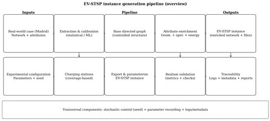
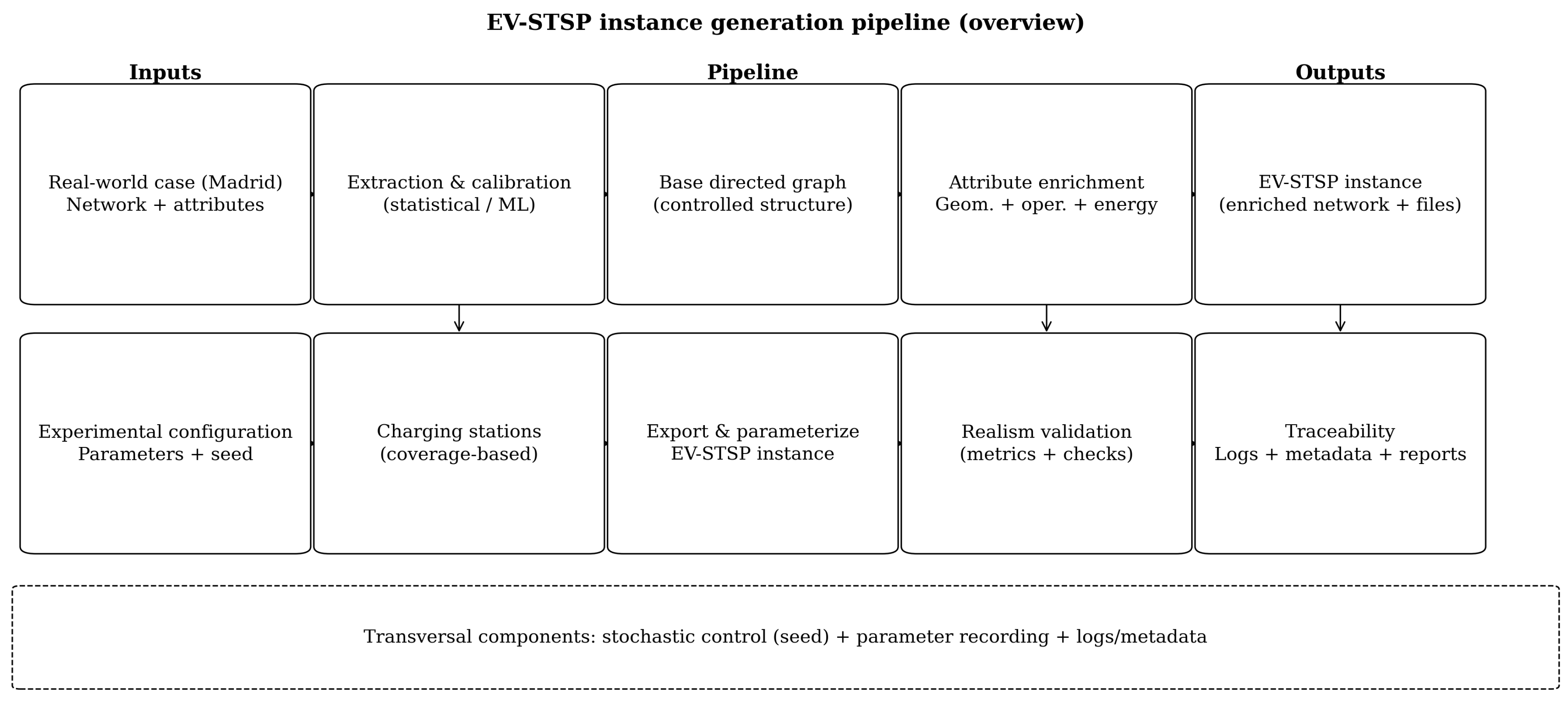
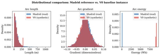
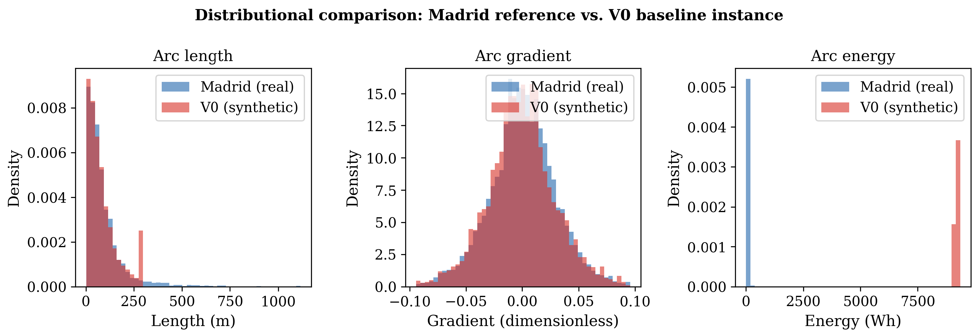
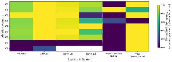
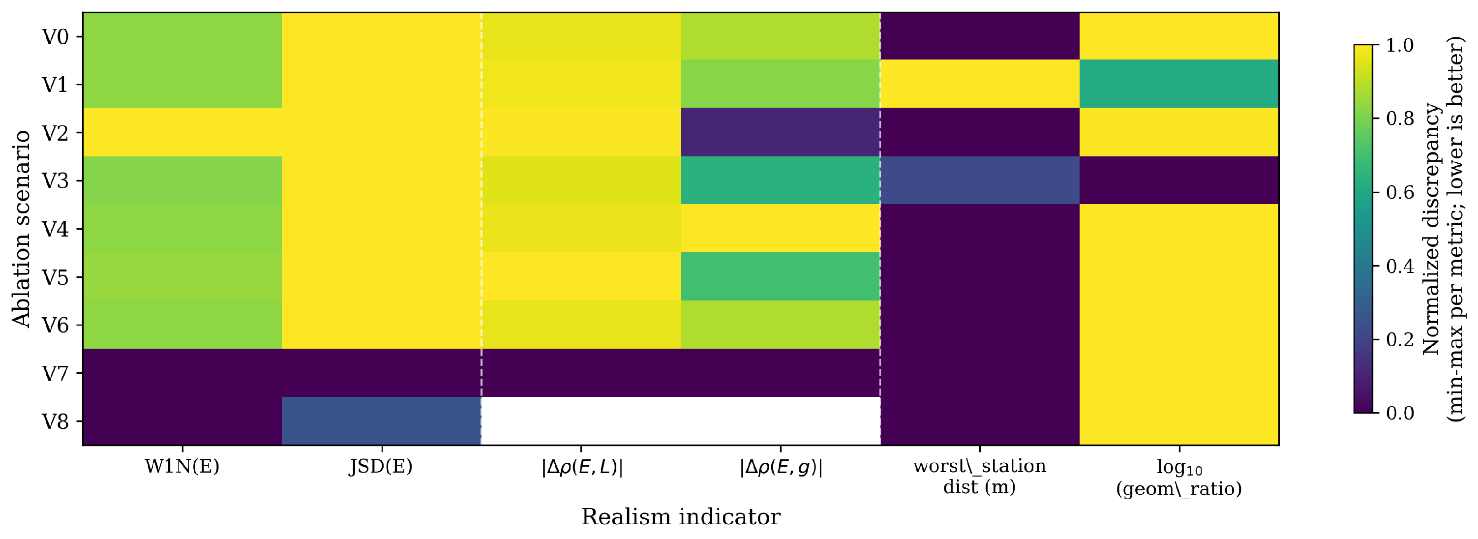
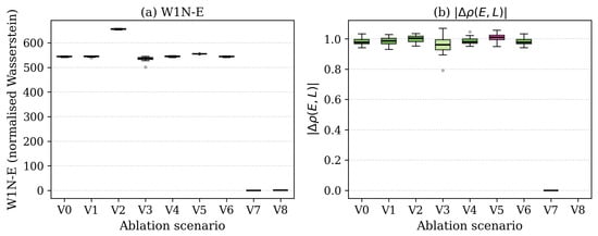
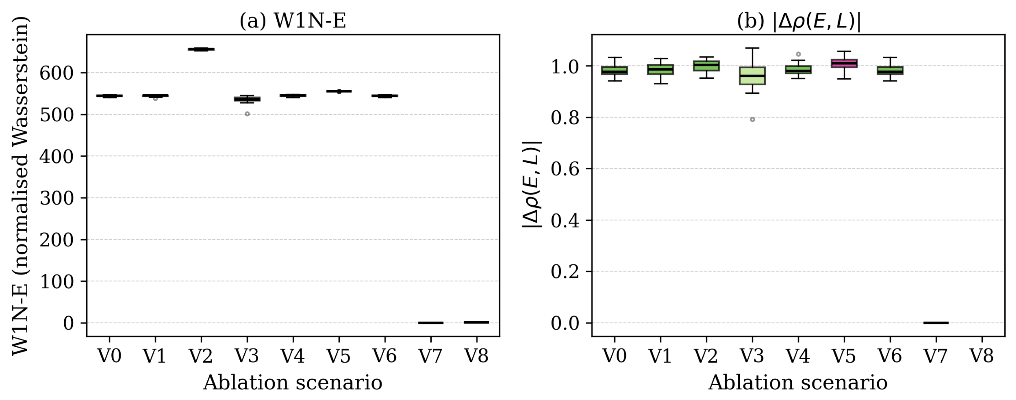
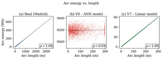

Disclaimer/Publisher’s Note: The statements, opinions and data contained in all publications are solely those of the individual author(s) and contributor(s) and not of MDPI and/or the editor(s). MDPI and/or the editor(s) disclaim responsibility for any injury to people or property resulting from any ideas, methods, instructions or products referred to in the content. |
© 2026 by the authors. Licensee MDPI, Basel, Switzerland. This article is an open access article distributed under the terms and conditions of the Creative Commons Attribution (CC BY) license.