Learning Bi-Objective Bayesian Network Structure from Data Using Particle Swarm Optimization

Abstract

This paper proposes a bi-objective approach to address the data-driven Bayesian network structure learning problem. The objectives considered for optimization are minimum description length (MDL) and misclassification. An algorithm based on the well-known multi-objective particle swarm optimization (MOPSO), called MOPSO-BN, is used to tackle the bi-objective learning problem. Furthermore, a strategy for preference handling from the Pareto front that selects the nearest model to a reference point is proposed. Finally, this bi-objective approach is compared against a single-objective approach. Numerical results show how this multi-objective approach is highly efficient at competitive Bayesian networks with a balanced trade-off between MDL and misclassification.

1. Introduction

Bayesian networks (BNs) are probabilistic graphical models that represent dependencies among random variables via a directed acyclic graph (DAG) [1]. Their ability to simultaneously support prediction, classification, inference, and visual interpretation of causal relationships has made them a widely adopted tool in many applications, including medicine, fault diagnosis, and decision-making [2].

Learning a BN structure from data is a combinatorial optimization problem of considerable difficulty. The number of possible DAG structures grows super-exponentially with the number of variables n according to Robinson’s formula [3]: with $n=10$ variables, there are already more than $4\times {10}^{18}$ candidate structures, and exhaustive evaluation becomes completely infeasible beyond $n\approx 6$. This explosive growth of the search space is the central computational challenge motivating the use of metaheuristics in BN structure learning. Existing approaches can be broadly divided into constraint-based methods [2], which use conditional independence tests to prune the search space, and search-and-score methods [4,5,6], which combine a scoring function with a search strategy to navigate the DAG space. This paper focuses on the second category.

Among scoring functions, the minimum description length (MDL) principle [7] has been widely adopted for BN structure learning. MDL balances model fit against structural complexity through a penalized log-likelihood, favoring compact models that avoid overfitting. However, a fundamental limitation of MDL as a sole optimization criterion is that it measures the global reconstruction error of the BN over all variables in the domain, rather than the local prediction error for the class variable [8]. As a consequence, the BN structure that minimizes MDL is not necessarily the one that minimizes misclassification rate, and vice versa. This discrepancy defines a clear technical gap: existing search-and-score methods that optimize MDL alone cannot simultaneously guarantee good classification performance, yet no prior work has explicitly and jointly optimized these two conflicting objectives in a principled bi-objective framework.

This paper addresses this gap by proposing MOPSO-BN, a multi-objective particle swarm optimization algorithm that simultaneously minimizes MDL and misclassification rate as two conflicting objectives. The key contributions of this work are as follows: (1) a graphical demonstration of the discrepancy between MDL and misclassification through exhaustive evaluation of all possible DAG structures in low-dimensional datasets; (2) the MOPSO-BN algorithm, which produces a Pareto front of non-dominated BN structures that explicitly trade off data compression against classification accuracy; (3) a preference-handling strategy that selects the solution nearest to a reference point from the Pareto front; and (4) a comparative evaluation against Naïve Bayes, TAN, and hill-climbing BNs on 20 real-world datasets. Unlike existing single-objective methods, MOPSO-BN provides the end-user with a set of structurally interpretable BN classifiers that balance both objectives, preserving the representational and inferential advantages of BNs alongside competitive classification performance.

The remainder of this paper is organized as follows: Section 2 describes the proposed method. Section 3 presents experiments and results. Section 4 summarizes the findings and proposes future work.

1.1. Literature Survey

Many methods have been proposed to learn the structure of BNs for classification purposes. One approach is based on the Naïve Bayes (NB) classifier. In [8], for instance, the authors propose the tree-augmented NB (TAN) approach, which approximates the relationship between attributes using a tree structure. In a TAN-based model, the class variable has no parents, and each attribute has as parents the class variable and at most another attribute; this approach does not consider the possibility of variables correlated with several variables. The work of Cerquides and Mántaras [9] improves TAN-style classifiers by defining a conjugate distribution called a decomposable distribution. Other authors have proposed methods to alleviate shortcomings of TAN-based classifiers [10,11,12,13,14].

The work of Grossman and Domingos [15] proposes a method for learning BN classifiers by maximizing the conditional likelihood of the class variable; they conclude that their approach produces better class probability estimates than maximum-likelihood approaches such as NB and TAN. Nevertheless, since the learned structures are not shown, it is unclear what the models’ complexity is (i.e., the number of arcs). The work of Madden [16] compares NB, TAN, and BNs learned using the K2 algorithm [17] as a search procedure with the BDeu metric [4] (that is, a refinement of the K2 metric) as a scoring function, versus a BN learned using hill-climbing search with MDL as a score function. The results show that BN-K2 classifiers significantly outperform NB and are comparable to TAN’s performance; the advantages of BNs over TAN point to representational power and complexity. Previous work shows that even if a BN exhibits good classification performance, other algorithms can outperform it. Nevertheless, improving the performance of BN classifiers is a topic with clear potential for research.

The work of Gheisari et al. [18] introduces two automata-based algorithms for BN learning. First, to measure the quality of their constructed networks, they use the BIC metric, which is considered equivalent to MDL [19]. Additionally, they analyze the classification accuracy of their proposed algorithm on 25 datasets by using a scoring function called classification rate. However, they do not show the models obtained, and the learning process does not integrate searching for optimal structure with assessing classification performance.

Regarding the learning problem of a BN structure using evolutionary algorithms (EAs), we list some representative examples. The work of Fang et al. [20] presents an algorithm for learning the structure of Bayesian networks using a genetic algorithm, which employs concepts of Markov blankets and equivalence in Bayesian network structures, and the Bayesian Dirichlet equivalent uniform (BDeu) scoring metric. The authors claim that their proposed method outperforms on datasets with many variables, but they do not show the induced structures.

In [21], the performance of a genetic algorithm (GA) is compared against two novel population-based, stochastic search algorithms; three different scoring functions are used, and the results show that their proposed algorithm can find structures similar to the original one when the order of the nodes is taken into account. In [22], a novel algorithm based on immune binary particle swarm optimization (PSO) and MDL as fitness function is proposed. Experiments show that the fitness function quality is superior in PSO compared to a GA. The work of Kuo et al. [23] applies MDL in a PSO-based algorithm to learn BN structures. They conclude that their proposed method (PSO-MDL) outperforms support vector machines (SVMs) and Weka’s BayesNet procedures [24] (in terms of classification accuracy). In [25], a hybrid algorithm combining the maximal information coefficient with a binary PSO is proposed. The experimental results show that the algorithm performs better than five other state-of-the-art algorithms without a given node ordering.

In [26], the authors proposed a bi-objective evolutionary Bayesian network structure-learning method. The authors argue that the score-based approach of learning is bi-objective due to the two terms of the scores, log-likelihood and complexity, so they proposed a structure learning method via skeleton constraints (BBS) for medium-scale networks. However, BBS and related methods focus on recovering the dependency structure among variables rather than on optimizing classification performance, a key distinction from our proposed MOPSO-BN.

Our own previous work [27,28], presents a bi-objective method, named the nondominated sorting genetic algorithm for learning Bayesian networks (NS2BN), which is based on the well-known NSGA-II algorithm. To avoid complex models that overfit the data, NS2BN employs two MDL terms as objectives: the log-likelihood, which measures goodness-of-fit, and a term that penalizes complex models. That problem is known as the bias–variance dilemma. The works of [26,27,28] are focused on learning structures that reflect the relationships between variables but do not necessarily focus on BNs for classification tasks.

The work of Ross and Zuviria [29] uses a multi-objective genetic approach to learn dynamic BNs from data, balancing likelihood and complexity. This work focuses on modeling biological phenomena that typically involve low-connectivity networks with at most four parents. They propose a learning methodology that allows an intuitive, user-defined structure for solution networks. In general, works based on evolutionary algorithms (EAs) and MDL do not report the learned network and are mainly designed to recover the original network, except for the approach of Kuo et al. [23], which uses classification accuracy as the performance metric.

Recent work has continued to explore diverse strategies for BN structure learning, combining heuristic search, regularization techniques, and hyper-heuristic frameworks. The work of Sun et al. [30] proposes OP-PSO-DE, a hybrid algorithm that combines Particle Swarm Optimization (PSO) and Differential Evolution (DE) with opposition-based learning to accelerate convergence in BN structure learning. The key idea is to generate opposite solutions alongside regular solutions at each iteration, effectively halving the search space and efficiently guiding particles toward the global optimum. The authors apply a binary mutation with a probability difference operator to handle the discrete nature of the DAG search space, and adopt an adaptive inertia-weight strategy based on the swarm’s success rate. The experimental results on CANCER, ASIA, and INSURANCE networks show that OP-PSO-DE converges significantly faster than PC-PSO and BNC-PSO, achieving competitive BIC scores, particularly in small-sample regimes. However, the authors acknowledge that premature convergence occurs as network scale increases, limiting its applicability to large networks.

The work of Fallahnejad et al. [31] introduces an Elastic Net-based K2 algorithm (EN-K2) for BN structure learning that addresses the K2 algorithm’s sensitivity to node ordering. Their approach first estimates the Markov Blanket (MB) of each variable using Elastic Net-penalized regression, which balances L1 and L2 regularization to improve stability in the presence of correlated predictors. A novel dependency-based scoring function is then applied to identify candidate parents within each estimated MB through pairwise comparisons, and the resulting candidate sets are passed as input to the K2 algorithm. Experiments on ASIA, ALARM, CAR, and MIDWAY datasets demonstrate that EN-K2 detects more correct edges and substantially reduces reversed and additional edges compared to the Lasso-based and Ko and Kim methods, particularly as sample size increases.

On the heuristic and metaheuristic side, recent work has proposed novel search strategies for discrete BN structure learning. Yang et al. [32] proposed to use scatter search to learn BN structures by combining diversification and intensification strategies in the DAG space, showing competitive results against hill-climbing and genetic algorithm baselines. He et al. [33] introduced a neighboring complete-node-ordering search algorithm that determines the topological ordering of variables and uses hill-climbing to find the best network structure within each ordering. Liu et al. [34] proposed an improved Harris Hawks Optimization algorithm with genetic operators for BN structure learning, demonstrating competitive BIC scores on standard benchmark networks. Wang et al. [35] proposed a novel skeleton learning method based on dynamic thresholds and triangle-breaking combined with hill-climbing, achieving better structural accuracy than standard hybrid approaches. These reports confirm that heuristic search remains an active and productive research direction for BN structure learning, and that population-based methods continue to offer advantages over purely greedy approaches in terms of solution quality and diversity.

The work of Dang et al. [36] proposes a hyper-heuristic algorithm for BN structure learning that integrates both soft and hard structural constraints. Soft constraints are derived from a feature-selection-based local learning method that mines conditional independence information to define restricted search spaces, while hard constraints are provided by expert domain knowledge. These constraints are incorporated into an Exponential Monte Carlo with Counter (EMCQ) hyper-heuristic framework that manages a library of low-level operators, including mutation, neighborhood hill-climbing, learning, restart, and expert-knowledge operators. The experimental results on six standard BN benchmarks from the BNLEARN repository—ranging from 37 to 441 nodes—show that EMCQ-HH achieves superior BIC scores and F1-scores compared to PC-Stable, GS, F2SL, MMHC, and BNC-PSO, demonstrating stronger robustness in large-scale and limited-data scenarios.

Beyond algorithmic advances in BN structure learning, recent work has demonstrated the practical value of Bayesian probabilistic modeling in real-world engineering applications, further motivating the dual objectives pursued in MOPSO-BN.

Yan et al. [37] propose a probabilistic fault diagnosis framework for bridge expansion joints in small and medium bridges using a convolutional neural network with Bayesian deep ensemble (CNN-BDE). Their method quantifies predictive uncertainty via a weighted ensemble of independently trained CNNs, with each model’s contribution determined by its negative log-likelihood on a validation set. An adaptive inter-class variance regularization term is introduced to enhance feature discrimination under noisy, small-sample conditions. Experiments on real-world acoustic data show that CNN-BDE achieves higher diagnostic accuracy and better uncertainty calibration than MC dropout, standard deep ensembles, and Gaussian process classifiers. This work illustrates how Bayesian ensemble strategies can yield robust and interpretable probabilistic outputs in safety-critical classification tasks with limited labeled data—a challenge structurally analogous to BN structure learning in small or medium-dimensional datasets.

Li et al. [38] address the problem of predicting typhoon-induced dynamic responses on long-span bridges by proposing CNN-BiLSTM-EDE, an explainable deep ensemble model that integrates convolutional and bidirectional LSTM layers within a probabilistic framework. The deep ensemble scheme produces a conditional predictive distribution over bridge responses, while Shapley additive explanations (SHAP) are incorporated to reveal the marginal contributions of input features, identifying the mean wind speed and wind direction angle as the most influential factors. Validated on decade-long typhoon datasets from a kilometer-scale bridge, the model outperforms four probabilistic benchmark methods in both prediction accuracy and uncertainty quantification. This study highlights the growing importance of combining predictive accuracy with structural interpretability and uncertainty quantification in data-driven engineering models—properties that are also central to the motivation of MOPSO-BN, which seeks BN structures that simultaneously optimize classification performance and model compactness.

In general, the recent literature confirms two converging trends: (1) the increasing use of population-based and metaheuristic algorithms for BN structure learning in discrete domains, where gradient-based continuous methods are not directly applicable; and (2) a growing interest in multi-objective formulations, as evidenced by works such as [26] and our own previous contributions [27,28], that go beyond single-score optimization. Our proposed MOPSO-BN is positioned at the intersection of both trends, contributing a principled bi-objective PSO-based framework that, unlike existing multi-objective BN learning methods, explicitly optimizes classification performance as a second objective alongside MDL, exploiting both the representational and classification capacities of BNs simultaneously.

1.2. Main Contribution

Even though there are multiple approaches to tackle the data-driven Bayesian network structure learning problem, existing solutions have not deeply explored the capacities of BNs, their graphical power for explaining the phenomenon under investigation, the relations among the random variables, or their ability to be used for classification purposes.

The core objective of this work is to propose an algorithm, MOPSO-BN, based on the well-known multi-objective particle swarm optimization (MOPSO), to identify a set of competitive Bayesian networks by minimizing both objectives: data compression using MDL and misclassification.

The choice of PSO as the underlying metaheuristic is motivated by complementary reasons. First, PSO has demonstrated competitive performance on BN structure-learning problems [22,23,30], demonstrating its ability to efficiently explore large combinatorial search spaces while avoiding premature convergence. Second, PSO is particularly well-suited for population-based search in binary spaces since its velocity-position update mechanism can be naturally adapted to handle adjacency matrix representations of BN candidates through a sigmoid transformation [39], as described in Section 2.2.3. Third, compared to other metaheuristics such as genetic algorithms (GAs), PSO requires fewer operator-specific parameters and is simpler to implement while maintaining competitive search performance [23]. Fourth, and most critically for our bi-objective formulation, PSO extends naturally to multi-objective settings through the MOPSO framework [40,41], where the concepts of personal best (pbest) and global best (gbest) can be redefined using Pareto dominance and hypervolume contribution, respectively, enabling effective approximation of the Pareto front. This last property distinguishes PSO from simpler single-objective heuristics and makes it a principled choice for simultaneously optimizing MDL and misclassification. Finally, the work of Sun et al. [30] further confirms that PSO-based algorithms for BN structure learning remain competitive against more recent alternatives, reinforcing the suitability of PSO as the backbone of our proposed method.

The main contributions of this paper are summarized as follows:

• The discrepancy between the MDL and the classification error was graphically demonstrated through the exhaustive evaluation of the set of possible BN candidates in low-dimensional instances.
• A multi-objective bio-inspired algorithm called MOPSO-BN was proposed to exploit the advantages of the shortest description of the original data, using MDL and expected classification.
• A set of resultant networks was obtained, which presents a trade-off between MDL and misclassification. They can be helpful in inference, classification, and explaining the relationships among the variables under investigation.
• A strategy to select a BN from a set of solutions in a Pareto front was explored, and the obtained solution was compared with a single objective algorithm.

In summary, our work suggests a bi-objective approach to addressing the BN structure learning problem, with objectives including MDL and misclassification rate.

The metaheuristic used in this work is based on PSO due to its well-documented effectiveness in multi-objective combinatorial optimization, its natural compatibility with binary solution representations for DAG-based BN structures, and its straightforward extension to the MOPSO framework, which provides a principled mechanism for Pareto front approximation through hypervolume-based leader selection [40].

2. Proposed Method

This section describes the proposed method and summarizes key fundamentals of BNs, including the multi-objective and non-dominated concepts.

2.1. Bayesian Networks

Formally, a BN [1] is represented as a pair $(G,\Theta )$, where G is a directed acyclic graph (DAG), which can be expressed by $(U,E_G)$; U is the set of nodes or random variables (denoted by $\{X_1,\dots ,X_n\}$), and $E_G$ is the set of arcs that represents the probabilistic relationships among these variables. The parents of $X_i$ are denoted by $P{A}_i$; $X_i$ is independent of its non-descendant variables given its parents. We denote as $\Theta$ the conditional probability distributions $P\left(X_i\right|P{A}_i)$ for each $X_i$. The joint probability distribution can be recovered from local conditional probability distributions as $P\left(X_1,\dots ,X_n\right)={\prod }_{i=1}^{n}P\left(X_i\right|P{A}_i)$.

2.2. Bi-Objective Bayesian Network Structure Learning

We divide the proposed method into three levels, shown in Figure 1, and described in detail next.

Figure 1. Diagram of the proposed method.

2.2.1. Input Level

As input to our proposed algorithm, we use a dataset represented as an $m\times n$ matrix, where m is the number of cases (or examples) and n is the number of attributes. As a preprocessing step, continuous variables must be discretized; for this, we use the Class-Attribute Interdependence Maximization (CAIM) algorithm [42], implemented in the Weka data mining software [24]. We delete records with missing data.

2.2.2. Start Level

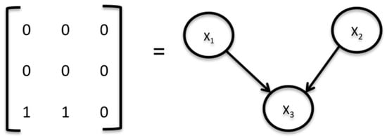
Our method is a population-based algorithm that is part of swarm intelligence (SI). The population is called a swarm: a set of N particles or solutions, each randomly generated. In our case, particles represent BN candidates. We use an adjacency matrix to represent each candidate structure (particle), as shown in Figure 2.

Figure 2. Example of an adjacency matrix and its corresponding BN according to [28].

Every BN candidate must be a DAG, meaning it cannot contain any directed cycles. If the optimization process generates a network with one or more cycles, it must be repaired before evaluation. We use a repair operator that modifies the adjacency matrix by replacing specific values when a cycle is identified. Three types of cycles can occur:

• Self-cycle: This happens when a node has a directed arc pointing to itself, i.e., a 1 in the diagonal of the adjacency matrix. The repair strategy simply replaces that 1 with a 0, eliminating the self-loop.
• Bi-directional cycle: This occurs when two nodes mutually influence each other, meaning there is an arc from node $v_i$ to node $v_j$ and simultaneously an arc from $v_j$ to $v_i$. Since this creates a cycle of length 2, the repair operator randomly removes one of the two conflicting arcs by setting the corresponding matrix entry to 0.
• General cycle: This involves a directed path of length greater than 2, where a sequence of nodes $v_1\to v_2\to \cdots \to v_k\to v_1$ forms a closed loop. To resolve it, the repair operator first identifies the path responsible for the cycle and then randomly removes one of the offending arcs, breaking the cycle while preserving as much of the network structure as possible.

The cycle repair mechanism acts as a constraint projection operator: it maps each infeasible position back into the feasible DAG space by removing the minimum number of arcs needed to eliminate the detected cycle [43]. Although the repair step creates a transient discrepancy between the stored velocity ${\overrightarrow{v}}_i$ and the repaired position ${\overrightarrow{x}}_i$, this discrepancy is self-correcting: in the next velocity update (Equation (3)), both attraction terms $({\overrightarrow{pbest}}_i-{\overrightarrow{x}}_i)$ and $(\overrightarrow{gbest}-{\overrightarrow{x}}_i)$ are recomputed relative to the repaired position, so the particle automatically re-aligns its trajectory toward the personal and global best solutions from its new feasible structure [39]. The random selection of which arc to remove when multiple arcs contribute to a cycle is a deliberate choice that introduces controlled structural diversity into the repair process, preventing all particles from following identical repair trajectories and thus reducing the risk of premature convergence. As the swarm converges and velocity magnitudes decrease—driven by the inertia weight $w=0.4$, which favors exploitation over exploration in later stages—cycle violations become less frequent, and the influence of the repair operator on the search trajectory diminishes naturally. The repair mechanism, therefore, preserves the fundamental PSO dynamics while ensuring that each evaluated candidate corresponds to a valid DAG.

2.2.3. Algorithm Level

Inspired by [40,41], we propose a bi-objective particle swarm optimization algorithm, MOPSO-BN. In the next sections, we provide multi-objective concepts relevant to our proposed algorithm. Section 2.4 presents the objectives to be optimized, followed by an explanation of MOPSO-BN.

2.3. The Multi-Objective and Non-Dominated Concepts

According to Deb and Kalyanmoy [44], a multi-objective optimization problem (MOOP) can be seen as a search problem that aims to minimize or maximize two (or more) objectives that are in conflict. A MOOP can be formalized as $\overrightarrow{f}\left(\overrightarrow{x}\right)=[f_1\left(\overrightarrow{x}\right),f_2\left(\overrightarrow{x}\right),\dots ,f_l\left(\overrightarrow{x}\right)]$, where $\overrightarrow{x}=[x_1,\dots ,x_n]$ is a n-variable decision vector, $\overrightarrow{f}$ is the set of objective functions to be minimized or maximized, and l is the number of objectives.

We base our proposed algorithm on the concept of dominance [40]. Before moving forward, we provide the following definition. A solution $x_1$ dominates a solution $x_2$ (denoted by $x_1⪯x_2$) if the solution $x_1$ is not worse than $x_2$ in all objectives and it is better than $x_2$ in at least one objective. When we are dealing with MOOPs, there is no single optimal solution; instead, there is a set of alternative solutions that have no solution that dominates them all when all objectives are considered. The set of non-dominated solutions is called a Pareto optimal set, and its corresponding objective function values are known as the Pareto front [44].

2.4. Scoring Metrics

As we pointed out before, a BN is a graphical model representing probabilistic relationships among variables of interest; its qualitative part, or structural model, provides a visual representation of the phenomenon under investigation. These are some of its main advantages. Therefore, one of our main interests is to exploit the BN’s representational power and classifier capacity using a search-and-score approach. However, it has been demonstrated that other models, such as NB and TAN, outperform BNs in classification, as we discuss in Section 1.1.

The MDL metric has been widely used for learning the structure of a BN from data. However, it has been discussed that a BN with an acceptable MDL score is not always a good classifier [45] due to MDL globally measuring the error of the learned BN across all variables in the domain, rather than the error in predicting the variable class (Section 3.2 shows this discrepancy graphically).

This subsection describes the metrics used in our bi-objective approach. MOPSO-BN seeks a competitive set of solutions that balance MDL ($f_1$) and misclassification ($f_2$). Solutions that entail this trade-off can support inference and classification. The scoring metrics are described below:

MDL is defined by [46] as follows:

$$f_1=-logP\left(D\right|\Theta )+{\displaystyle \frac{k}{2}}logn$$

(1)

where D is the dataset, $\Theta$ represents the parameters of the model, k is the dimension of the model, and n is the sample size. Parameter $\Theta$ is the corresponding local probability distribution for each node in the network, determined by each BN structure.

The first term of Equation (1), $-logP\left(D\right|\Theta )$, corresponds to the negative log-likelihood of the data given the model parameters $\Theta$. These parameters are estimated using the simple estimator procedure implemented in Weka [24], which computes the conditional probability tables (CPTs) of each node in the network from the data using relative frequencies with a small Laplace-style smoothing value ($\alpha =0.5$ by default) to avoid zero probabilities in cases where a particular combination of variable values does not appear in the dataset. Once $\Theta$ is estimated, the log-likelihood term is computed as

$$-logP\left(D\right|\Theta )=-{\displaystyle \sum _{j=1}^m}{\displaystyle \sum _{i=1}^n}logP\left(x_i^{\left(j\right)}\mid p{a}_i^{\left(j\right)},\Theta \right)$$

(1a)

where $x_i^{\left(j\right)}$ denotes the value of variable $X_i$ in instance j, and $p{a}_i^{\left(j\right)}$ represents the corresponding values of the parent variables of $X_i$ in that same instance. This decomposition follows directly from the conditional independence assumptions encoded in the BN structure, which allow the joint likelihood to be factored into local contributions from each variable, given its parents.

The model dimension (k) is given as follows.

$$k={\displaystyle \sum _{i=1}^m}{q}_i(r_i-1)$$

(1b)

where m is the number of attributes, $q_i$ is the number of possible configurations of the parents of variable $X_i$, and $r_i$ is the number of values of that variable.

The first term of Equation (1) measures the accuracy of the model (in terms of the likelihood of the data), and the second term measures its complexity. The complexity is proportional to the number of arcs, as shown in Equation (1b).

Equation (2) describes $f_2$, where $a_i$ represents the number of instances incorrectly classified in the i-th fold of the testing set, b is the total number of instances in the fold, and s is the number of folds ($s=10$ in our case). The misclassification rate is thus computed as the average classification error across all folds of an s-fold cross-validation procedure.

$$f_2={\displaystyle \frac{1}{s}}{\displaystyle \sum _{i=1}^s}{\displaystyle \frac{a_i}{b}}$$

(2)

The model parameters are computed using the simple estimator procedure implemented in Weka [24].

2.5. MOPSO-BN

The original PSO was designed to handle continuous search problems. In our approach, each candidate network solution is represented as a binary vector. We use a sigmoid function to map the vector of each particle in the swarm to 0 and 1 after updating the velocity vector [39], as shown in Algorithm 1 at lines 3 and 16.

The evaluation of the network candidate is based on two objectives. (i) MDL (Equation (1)) and (ii) misclassification (Equation (2)). Section 2.2.2 explains the representation and cycling-repair process. Our methodology is described in Algorithm 1. The initial $\overrightarrow{pbes{t}_i}$ corresponds to the first particle, while the hypervolume contribution of each particle serves to update $\overrightarrow{pbest}$. The hypervolume is a performance metric used in evolutionary multi-objective optimization [41]. The non-dominated particles are stored in a specified file (file A) beforehand. The maximum number of iterations ($ma{x}_{gen}$) must be specified as a stopping criterion for the algorithm.

To select the leader $\overrightarrow{gbest}$, we calculate the hypervolume contribution of the particles in file A, as can be seen in Section 2.5.1. We compute the new velocity and position of each particle in the population according to Equations (3) and (4) (see Algorithm 1), where three parameters determine the particle’s position: the current position $\overrightarrow{x_i}$, the previous best position $\overrightarrow{pbes{t}_i}$, and the velocity $\overrightarrow{v_i}$. w represents the inertia, which controls the impact through the velocity history and the current velocity. $C_1$ and $C_2$ are considered the learning factors. $C_1$ is the cognitive factor and represents the attraction that a particle has towards its success. $C_2$ is the social factor and represents the attraction that a particle has toward the success of its neighbors. Both factors are usually defined as constants.

Algorithm 1 MOPSO-BN

1: Initialize the generation counter with $t=0$ 2: Initialize randomly the position and velocity of each particle in swarm S 3: Transform the real position vector into a binary vector for each particle in swarm S through a sigmoid function 4: Repair the position vector if cycles are detected 5: Evaluate each particle in swarm S in the two objective functions 6: Select the initial $\overrightarrow{pbest}$ of each particle in swarm S 7: Insert non-dominated particles of the in swarm S in the file A 8: while  $t<ma{x}_{gen}$  do 9:      for $i=1$ to $\left|S\right|$ do 10:         Select gbest, compute velocity and position 11:     end for 12:     Compute the contribution of each particle to the hypervolume value of swarm S 13:     Compute the new velocity and position of each particle in the population. According following: $$\overrightarrow{v_i}=w\overrightarrow{v_i}+C_i\otimes r_1(\overrightarrow{pbes{t}_i}-\overrightarrow{x_i})+C_2{r}_2(\overrightarrow{gbest}-\overrightarrow{x_i})$$ (3) $$\overrightarrow{x_i}\leftarrow \overrightarrow{x_i}+\overrightarrow{v_i}$$ (4) 14:     Repair cycles 15:     Evaluate each particle in swarm S in the two objective functions 16:     Using the sigmoid function to transform the real position vector into a binary vector 17:     Update pbest particle 18:     Update non-dominated particles in file A 19:     $t=t+1$ 20: end while 21: Return A

It is important to mention that the work of [47] suggests that one of the critical issues in BN structure learning is the search procedure. This is why several proposed heuristics can address such a challenge. Although there are different ways to search for BN structures, we focus on the space of DAGs since their representation as adjacency matrices can facilitate the implementation of operators in a PSO-based algorithm, such as our MOPSO-BN. A problem with this search space is the global acyclicity constraint [48]; to overcome this obstacle, we use an operator that avoids cycles while maintaining the randomness of the particle when adding arcs that were eliminated due to cyclicity.

Another significant issue in the BN learning problem is parameter optimization; we use a simple estimator for classification, but the parameters depend on the sample size [24]. We defer learning BN parameters to future work; after running our proposed MOPSO-BN, we obtain the Pareto front, and a local search procedure further optimizes the parameters, improving our final results.

The computational cost of MOPSO-BN per dataset is determined by the number of fitness evaluations, $E_{total}=R\times I\times P=10\times 200\times 100=\mathrm{200,000}$, where each evaluation involves computing MDL (Equation (1)) and misclassification via 10-fold cross-validation (Equation (2)), with a cost of $O(s·N·{\sum }_{i=1}^n{q}_i·r_i)$ per particle. Although this represents a higher computational investment than deterministic methods such as NB, TAN, and HC-BN, this cost is justified by the population-based global search capability of MOPSO-BN and, most importantly, by the fact that it simultaneously optimizes two conflicting objectives, producing a Pareto front of non-dominated solutions that cannot be obtained by any single-objective deterministic method. Furthermore, since BN structure learning is typically performed offline prior to deployment, this one-time computational cost is amortized over the operational lifetime of the learned model.

2.5.1. Selection of pbest and gbest via Hypervolume Contribution

In a multi-objective setting, the classical PSO definitions of personal best (pbest) and global best (gbest) must be adapted since there is no longer a single scalar fitness value to compare solutions. In MOPSO-BN, both selections are based on the concept of hypervolume contribution, which measures the volume of the objective space dominated exclusively by a given solution with respect to a reference point $\overrightarrow{r}=(r_1,r_2)$, typically set to a point that is dominated by all solutions in the current archive (file A).

2.5.2. Personal Best (pbest) Update

The personal best ${\overrightarrow{pbest}}_i$ of particle i is updated by comparing its current position ${\overrightarrow{x}}_i$ against its previous best position using the concept of Pareto dominance. Specifically:

• If ${\overrightarrow{x}}_i$ dominates ${\overrightarrow{pbest}}_i$, then ${\overrightarrow{pbest}}_i$ is replaced by ${\overrightarrow{x}}_i$.
• If ${\overrightarrow{pbest}}_i$ dominates ${\overrightarrow{x}}_i$, then ${\overrightarrow{pbest}}_i$ remains unchanged.
• If neither solution dominates the other, the hypervolume contribution of each is computed with respect to the current archive A, and the solution with the greater contribution is selected as the new ${\overrightarrow{pbest}}_i$. This criterion favors solutions that contribute more to the diversity and spread of the Pareto front approximation.

2.5.3. Global Best (gbest) Selection

The global best $\overrightarrow{gbest}$ is selected from the external archive A, which stores the non-dominated solutions found so far across all particles and iterations. To select $\overrightarrow{gbest}$, the hypervolume contribution ${\Delta }_h\left(s\right)$ of each solution $s\in A$ is computed as

$${\Delta }_h(s)=\mathcal{H}(A,\overrightarrow{r})-\mathcal{H}(A\backslash \left\{s\right\},\overrightarrow{r})$$

(5)

where $\mathcal{H}(A,\overrightarrow{r})$ denotes the hypervolume of the archive A with respect to the reference point $\overrightarrow{r}$, and $A\backslash \left\{s\right\}$ is the archive without solution s. Thus, ${\Delta }_h\left(s\right)$ measures the exclusive hypervolume region dominated only by s. The solution with the highest hypervolume contribution is selected as $\overrightarrow{gbest}$ as it represents the most influential individual in shaping the current Pareto front approximation. This selection strategy encourages particles to move toward regions of the objective space that are both well-performing and diverse, balancing convergence and spread of the Pareto front throughout the optimization process [40,41].

3. Experimental Design and Results

We categorize our experiments into two steps. First, to show the discrepancy between MDL and misclassification, we evaluated all DAGs in low-dimensional domains. The second experiment tested our proposed algorithm using real-world datasets. The experiments and results are described below.

3.1. Datasets

For the experiments, we evaluated MDL and misclassification rate across seven low-dimensional datasets, thereby exhaustively considering all possible Bayesian network structures. Three of them were taken from the literature, each with $n=5$ variables, including the class variable: the Iris dataset with 150 instances, the Balance dataset with 625 instances, and the Sewell and Shah dataset with 10,318 instances [2,49]. The remaining four are synthetic datasets with $n=6$ and 10,000 instances, where all variables are binary; two were generated using a random probability distribution (RDP-1 and RDP-2) and the other two using a low-entropy distribution (LED-1 and LED-2) [50] (see details in Table 1).

Table 1. Characteristics of datasets in low-dimensionality domains.

Dataset	No. Classes	No. Features	No. Instances
Balance Scale	5	5	625
Iris	3	5	150
Sewell and Shah	2	5	10,318
RPD-1	2	6	10,000
RPD-2	2	6	10,000
LED-1	2	6	10,000
LED-2	2	6	10,000

For the second experiment, a set of 20 datasets from the UCI repository [49] is used. Continuous variables are discretized using Weka’s CAIM algorithm [24], and cases with missing values are removed. Table 2 describes the datasets.

Table 2. Characteristics of datasets of real-world domain.

Dataset	No. Classes	No. Features	No. Instances
Australian	2	14	690
Chess	2	36	3296
Cleve	2	11	296
CorrAl	2	6	128
crx	2	15	653
Diabetes	2	8	768
Flare	8	10	1389
German	2	20	1000
Glass2	2	9	163
Heart	2	13	270
Hepatitis	2	19	80
Lymphograph	4	18	148
Mofn-3-10	2	10	1324
Pima	2	8	768
Segment	7	19	2310
SoyBean-large	19	35	316
Tic-tac-toe	2	9	958
Vehicle	4	18	958
Vote	2	17	436
Waveform-21	3	21	301

3.2. MDL and Misclassification

In general, it is not possible to exhaustively evaluate all DAGs since the number of possible structures increases exponentially with the number of variables. It is possible to compute the number of DAGs as a function of the number of attributes n according to Equation (6); e.g., when $r\left(5\right)$, the number of possible structures, is $\mathrm{29,281}$ [3].

$$r\left(n\right)={\displaystyle \sum _{i=1}^n}{(-1)}^{i+1}\left({\displaystyle \genfrac{}{}{0pt}{}{n}{i}}\right)2^{i(n-1)}r(n-i)$$

(6)

We evaluate MDL and misclassification rate in the seven datasets described in Section 3.1. We apply the 95% non-parametric Mann–Whitney U test to compare the misclassification of the network with the minimum MDL value against the model with the best misclassification score.

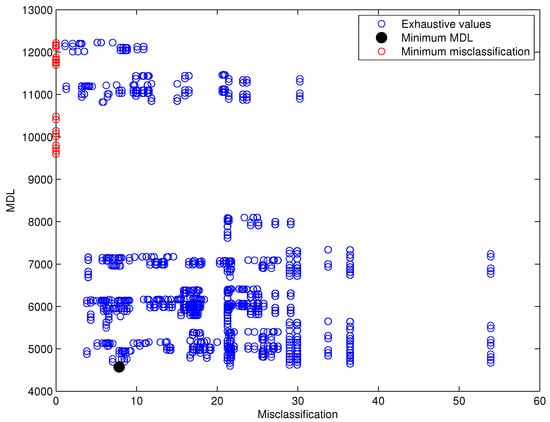
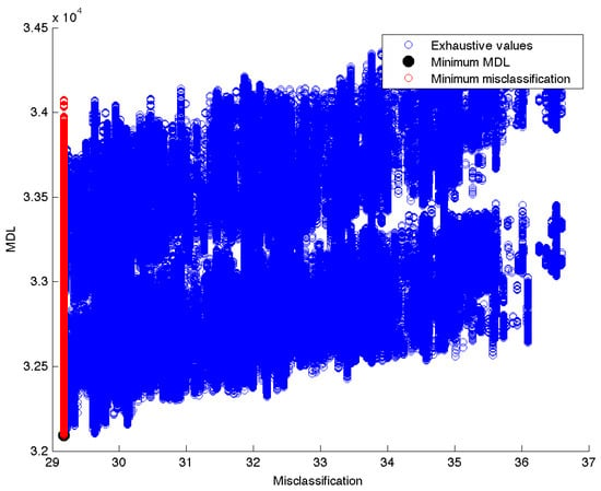
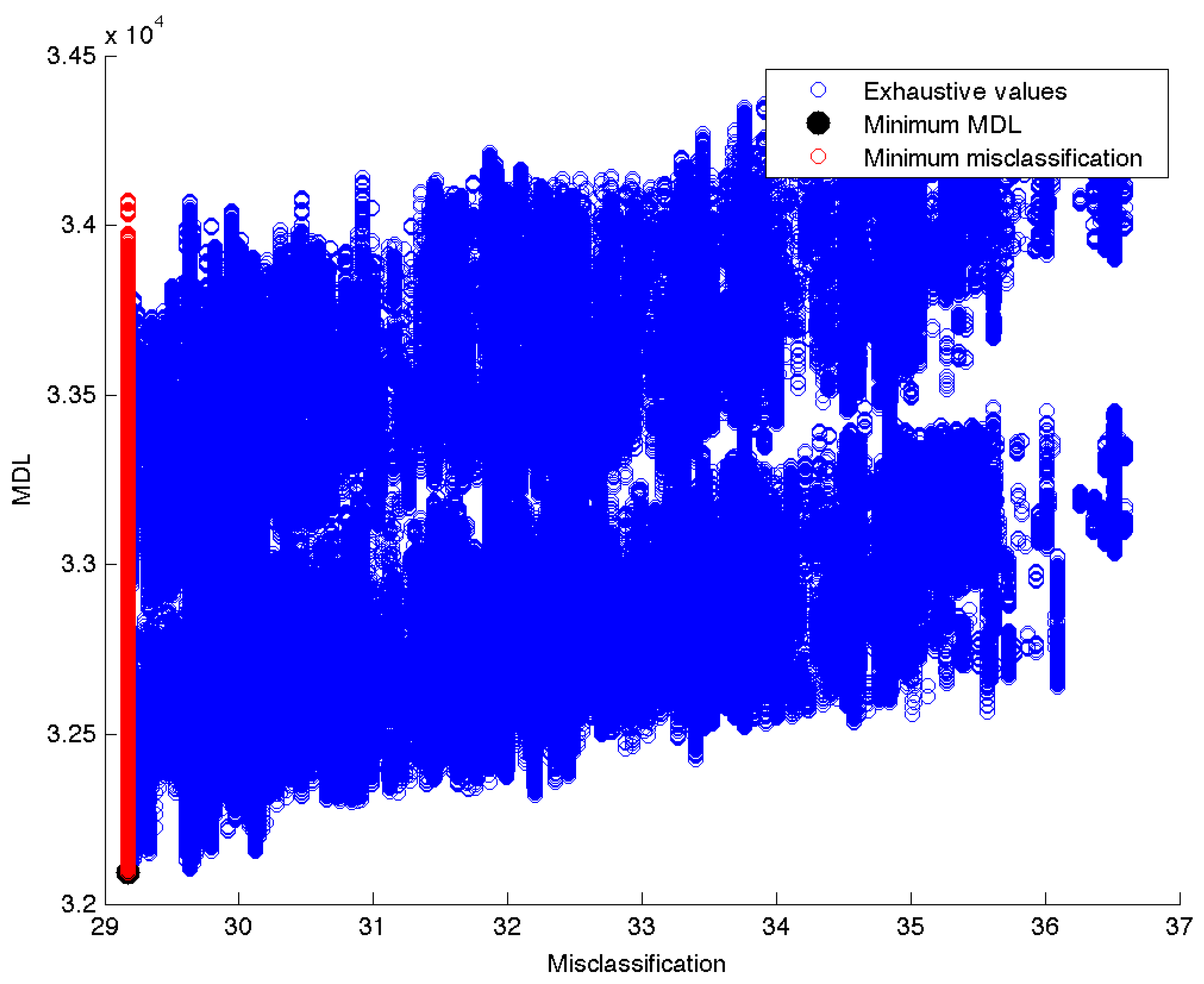
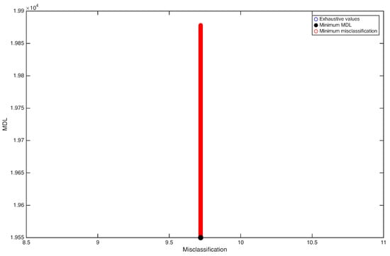
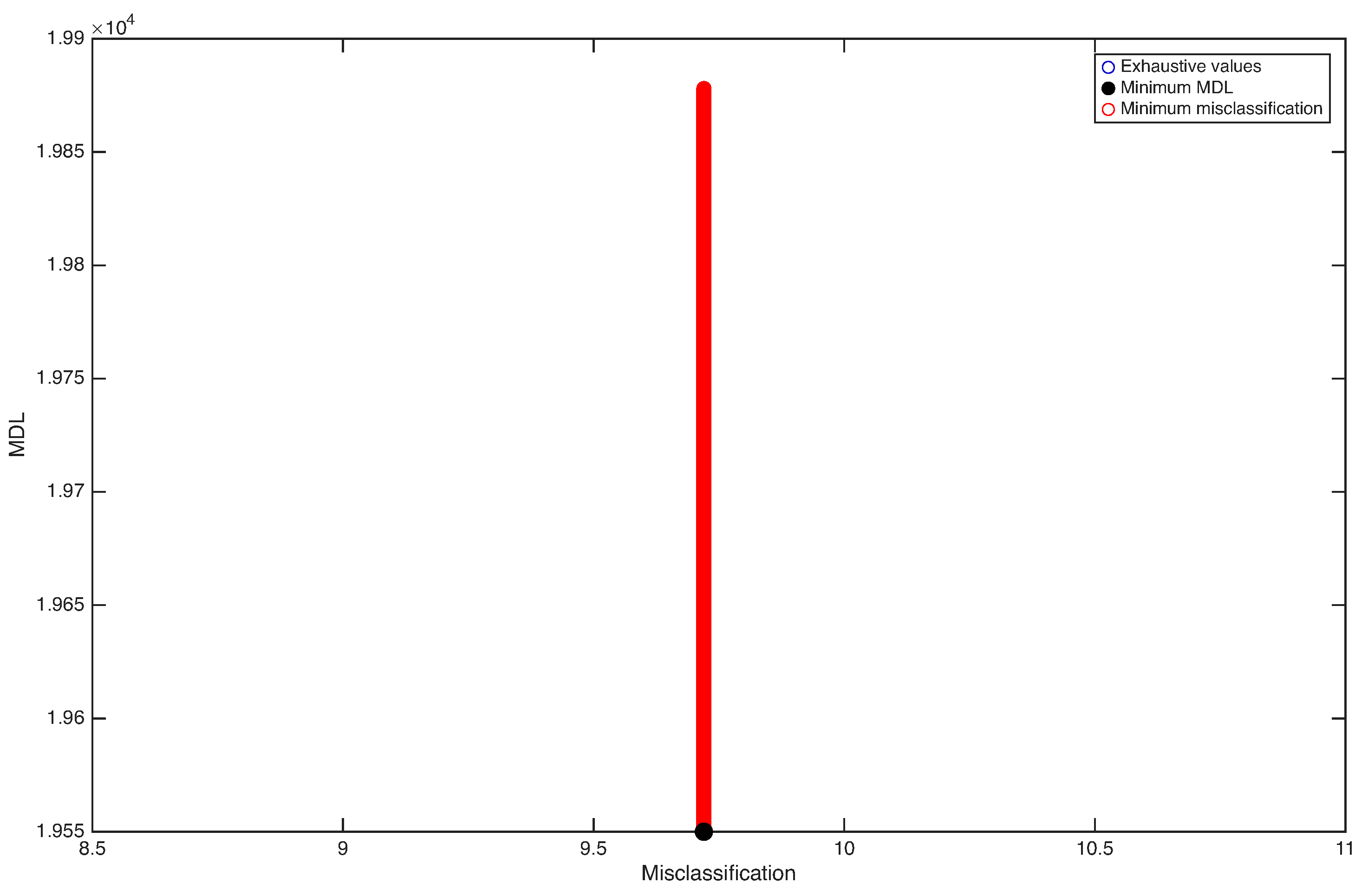
The following briefly explains how we present our results. Figure 3, Figure 4 and Figure 5 show an exhaustive evaluation of each BN structure. We plot misclassification (x-axis) vs. MDL (y-axis). The blue dots represent BN; the black dot represents the minimum value of MDL, while the red dots represent the minimum value of misclassification. It is possible to have more than one structure with the same value of MDL or misclassification, in which case dots may overlap, as is the case in Figure 4, where it is possible to see several BN structures with the same value of misclassification in contrast with different values of MDL, and in Figure 5, where the whole of BN structures has the same value of misclassification and different value of MDL.

Figure 3. Balance scale.

Figure 4. Random probability distribution 1 (RPD-1).

Figure 5. Low-entropy probability distribution 1 (LED-1). Red circles overlap the blue circles.

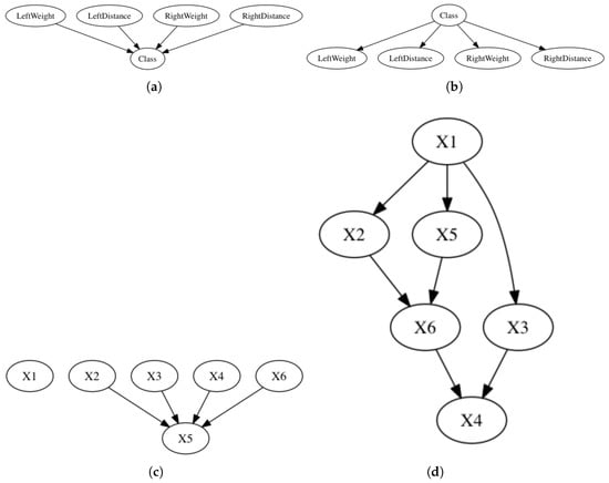
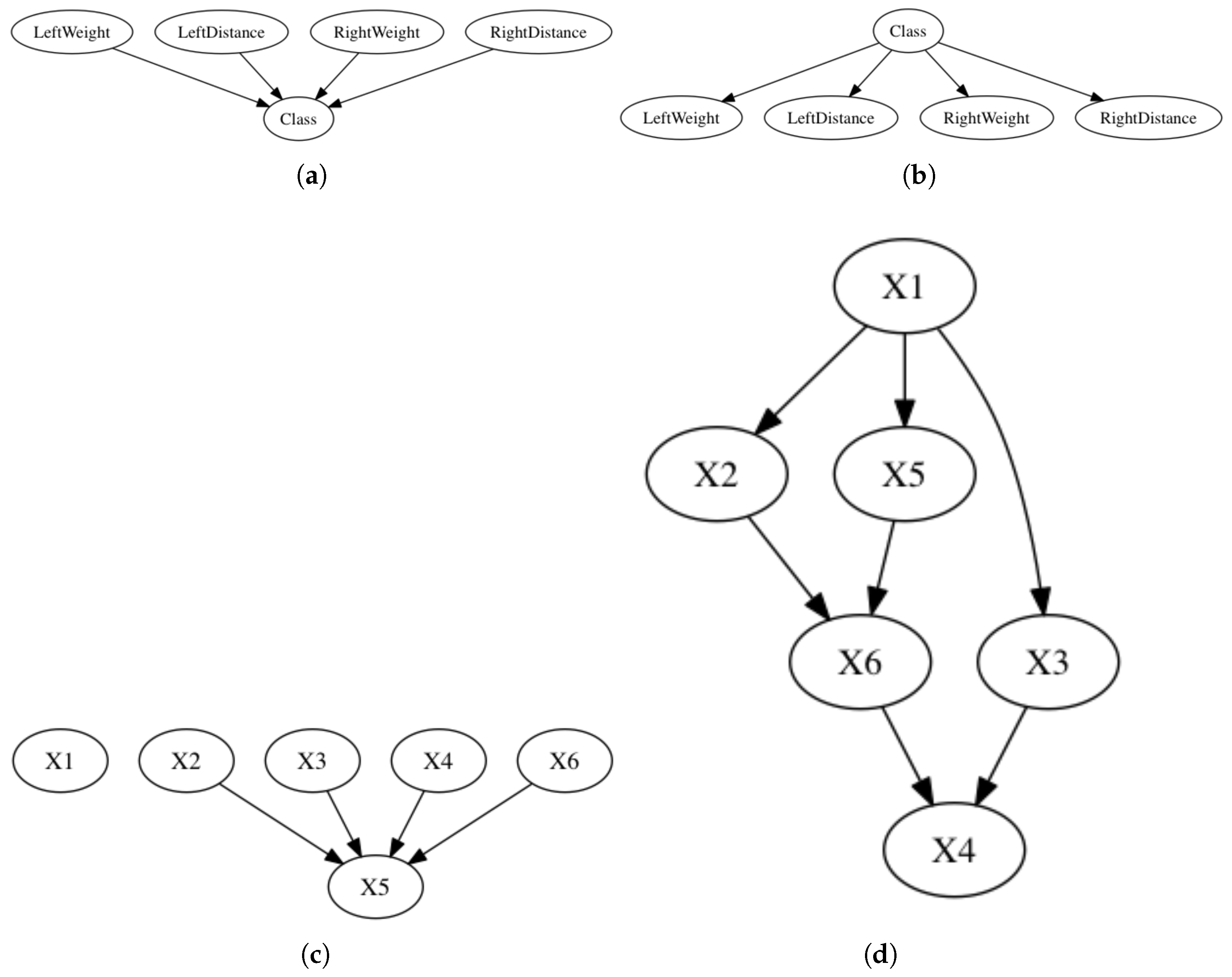
Table 3 compares performance among the seven tested datasets. We first identified the BN structure with the smallest MDL value; then, we compared it to the networks with the smallest misclassification rate. Since we have several networks with the same value of misclassification, we present the average structural difference (the difference regarding the arcs: reversed, missing, and extra, between the model with the smallest MDL value and the models with the minimum misclassification) and the average Kullback–Leibler (KL) divergence (computed as the ${log}_2$ of the ratio of the smallest MDL value network/the model with the minimum misclassification) to distinguish the distance and the difference among the networks. Figure 3 and Figure 6a,b present a visual comparison of the BN structures for two datasets: Balance Scale and RPD-1.

Table 3. Average structural difference and average Kullback–Leibler (KL) divergence between the model with the smallest MDL value and the networks with the minimum misclassification. Values in parentheses represent the standard deviation, and values in boldface mean the significant best value found.

Dataset	Reversed	Missing	Extra	Average KL Divergence	Minimum MDL Value		Minimum Misclassification Value
					MDL	Misclassification	MDL	Misclassification
1. Balance Scale	7.6889	0	3.9004	0.3891	4573.7254	7.83 (±0.46)	9599.5836	0.0 (±0.0)
2. Iris	3.2195	0.6293	3.9102	0.3558	529.3484	4.0 (±4.422)	655.1409	3.33 (±3.33)
3. Sewell and Shah	5.5323	0.9835	3.1405	0.0117	45,636.9539	19.94 (±1.18)	47,574.7018	19.84 (±1.33)
4. RPD-1	5.1296	1.4168	5.0337	0.0254	32,093.7447	29.17 (±0.85)	34,072.1691	29.17 (±0.85)
5. RPD-2	8.1888	1.2158	3.6749	0.0114	35,368.8459	15.24 (±0.55)	36,139.7766	15.24 (±0.55)
6. LED-1	0	0	8.8368	0.0010	19,277.8087	9.72 (±0.04)	19,277.8087	9.72 (±0.04)
7. LED-2	0	0	8.8368	0.0010	19,553.7187	9.79 (±0.03)	19,553.7187	9.79 (±0.03)

Figure 6. Graphs with the smallest values. (a) Network with the smallest value of misclassification and MDL from the Balance Scale dataset. (b) Network with the smallest value of MDL from the Balance Scale dataset. (c) Network with the smallest value of misclassification and MDL from the RPD-1 dataset. (d) Network with the smallest value of MDL from RPD-1.

Our experiment aims at showing the degree of discrepancy between MDL and misclassification graphically (see Figure 3, Figure 4 and Figure 5). We know that MDL measures the error of the BN across all variables in the dataset; thus, minimizing this error does not entail minimizing the local error in predicting the class variable given the attributes [8]. Some authors have explored the use of MDL to learn BN classifiers [15,16,23,51,52]. In this sense, our results suggest that since the BN with the smallest MDL value could have interactive effects with classification error, we do not need to observe statistically significant differences regarding misclassification (see Table 3). Other ways to learn BN classifiers include: (1) approximating the true joint probability distribution over the attributes and (2) classifying the class variable given the attributes. A standard approach to achieving the first method is to use a quality measure based on log-likelihood, as in MDL. For the second method, one can use prediction error as misclassification or as the conditional log-likelihood; this is typically not used directly in practice due to its computational complexity [15,53]. Our results show that it is possible to find several BNs with the same misclassification rate but different MDL values; hence, selecting one of them could lead to overfitting [16].

One of our primary goals is to learn BN structures that capture dependence, conditional independence, and even causal relationships among attributes; we wish to use this learned model for classification. Using the metrics mentioned above, this is in general not possible; e.g., we graph the networks at the extremes, that is, the network with the smallest value of misclassification but the worst value of MDL (see Figure 6c) and the network with the smallest MDL value (see Figure 6d). Although both models are equally valid regarding accuracy, Figure 6c could have less representational power in comparison with Figure 6d. This behavior highlights the conflict between both objectives [8,15,52].

Regarding the synthetic low-entropy datasets, as noted in [50], MDL tends to select simpler models and, hence, does not exploit the advantages of BNs (see Figure 5). Although several studies have exhaustively evaluated MDL in low-dimensional domains [2,16,47,52], they do not compare the learned models with respect to their structure. To address this discrepancy, we propose a bi-objective approach, evaluated in the next section.

3.3. The Trade-Off Between MDL and Misclassification

This section describes a set of experiments to test our proposed algorithm MOPSO-BN. The details of the dataset can be seen in Table 2.

For this experiment, which involves 20 real-world datasets of higher dimensionality where an exhaustive search is computationally infeasible, MOPSO-BN requires a parameter configuration. Given the high computational cost of running the algorithm—each configuration requires 10 independent runs with 20,000 evaluations across 20 datasets—a full factorial or grid search parameter analysis was outside the scope of this work. Instead, we followed the common practice in the evolutionary computation literature by starting from values reported in foundational PSO and MOPSO works [39,40,54,55,56,57] and then performing a manual sensitivity analysis by varying one parameter at a time while keeping the others fixed. The final values, $C_1=2.1$, $C_2=2.0$, $w=0.4$, $\mathrm{particles}=100$, and $\mathrm{cycles}=200$, were selected because they consistently yielded stable convergence and competitive Pareto fronts across the tested datasets. The inertia weight $w=0.4$ was chosen to favor exploitation over exploration in the later stages of the search, while $C_1$ and $C_2$ were kept close to theoretically recommended values that ensure particle convergence [39]. The swarm size and number of cycles were set to balance solution quality and computational feasibility. More systematic parameter tuning, such as using automatic configuration tools like irace, is part of our future work.

The algorithm performs 10 independent runs per database, for a total of $\mathrm{20,000}$ evaluations. Each run produces a set of trade-off solutions. The process of selecting the most suitable among them is known as preference handling. This work compares the bi-objective approach with other Bayesian network models, including NB, TAN, BNs learned using hill-climbing (HC-BN), and our selected BNs from the Pareto front. To find the latter, we propose a subsequent preference-handling approach: after accumulating the Pareto front across all ten independent runs, a single solution is selected using a reference-point strategy [40]. Let $\mathcal{F}={\left\{({\widehat{f}}_1^{\left(k\right)},{\widehat{f}}_2^{\left(k\right)})\right\}}_{k=1}^M$ be the set of M non-dominated solutions, where ${\widehat{f}}_1^{\left(k\right)}$ and ${\widehat{f}}_2^{\left(k\right)}$ are the MDL and misclassification values of solution k. Since both objectives differ substantially in magnitude, each is independently normalized to $[0,1]$ via min-max scaling over the accumulated Pareto front:

$${\tilde{f}}_j^{\left(k\right)}={\displaystyle \frac{{\widehat{f}}_j^{\left(k\right)}-{min}_l{\widehat{f}}_j^{\left(l\right)}}{{max}_l{\widehat{f}}_j^{\left(l\right)}-{min}_l{\widehat{f}}_j^{\left(l\right)}}},j\in \{1,2\},k=1,\dots ,M$$

(7)

The selected solution $k^{*}$ minimizes the Euclidean distance to the ideal reference point $\overrightarrow{r}=(0,0)$ in the normalized space:

$$k^{*}=arg\underset{k}{min}\sqrt{{\left({\tilde{f}}_1^{\left(k\right)}\right)}^2+{\left({\tilde{f}}_2^{\left(k\right)}\right)}^2}$$

(8)

This criterion assigns equal weight to both objectives after normalization, favoring solutions that balance data compression and classification accuracy without requiring any dataset-specific parameter tuning. The normalization bounds are computed from the accumulated Pareto front of each dataset, making the procedure fully self-contained and reproducible. The selected solution for each dataset is reported in Table 4 under the MOPSO-BN column.

Table 4. Mean of misclassification and standard deviation. Values in boldface mean the best values found. The p-value corresponds to the Mann–Whitney U test between HC-BN and MOPSO-BN. (+) means significance difference, (-) means significance difference in favor of HC-BN, and (=) means that there is no significant difference.

No.	Dataset	NB	TAN	HC-BN		MOPSO-BN		HC-BN vs. MOPSO-BN p-Value
				Misc	MDL	Misc	MDL
1	Australia	14.2 ± 4.03	14.94 ± 3.90	11.73 ± 0.00	5767.22	11.44 ± 0.04 (=)	6123.65	0.88076
2	Chess	12.15 ± 1.70	7.91 ± 1.39	4.38 ± 0.0	39,208.69	9.57 ± 0.35 (-)	46,253.37	0.00034
3	Cleve	17.13 ± 6.20	18.96 ± 6.77	26.24 ± 0.03	3900.49	10.75 ± 0.13 (+)	13,583.83	0.00116
4	Corral	12.95 ± 9.46	0.77 ± 3.19	0.0 ± 0.0	594.61	0.0 ± 0.0 (=)	590.47	0.9681
5	crx	14.39 ± 2.30	16.11 ± 2.70	12.40 ± 0.0	7705.44	7.96 ± 0.35 (+)	10,797.20	0.00168
6	Diabetes	26.61 ± 2.8	27.41 ± 3.3	22.39 ± 0.01	4768.37	19.00 ± 0.35 (=)	5599.08	0.09692
7	Flare	19.88 ± 3.47	17.35 ± 3.47	15.00 ± 0.01	6824.10	12.75 ± 0.45 (=)	11,204.16	0.1031
8	German	25.39 ± 4.31	27.93 ± 4.04	20.29 ± 0.01	18,002.210	13.40 ± 0.44 (+)	29,057.68	0.00318
9	Glass2	18.84 ± 8.68	20.63 ± 8.95	7.35 ± 0.0	1522.69	2.42 ± 0.76 (=)	3147.29	0.08186
10	Heart	17.26 ± 6.70	16.89 ± 7.30	14.81 ± 0.02	2357.38	9.62 ± 0.46 (=)	2695.59	0.07508
11	Hepatitis	13.96 ± 10.97	12.0 ± 11.64	2.5 ± 0.00	950.34	2.5 ± 0.79 (=)	959.19	0.79486
12	Lymphography	17.84 ± 10.61	18.93 ± 9.57	6.71 ± 0.02	3595.33	2.04 ± 1.71 (=)	11,832.99	0.19706
13	Mofn-3-10	14.66 ± 3.43	8.04 ± 2.63	9.66 ± 0.0	2228.48	2.33 ± 0.31(+)	2372.03	0.00018
14	Pima	24.31 ± 4.42	23.63 ± 3.94	22.38 ± 0.01	4768.37	19.39 ± 1.14 (=)	5325.07	0.28914
15	Segment	8.73 ± 1.70	4.73 ± 1.49	5.38 ± 0.0	57,877.24	4.22 ± 0.51 (=)	49,573.03	0.22628
16	Soybean-large	8.17 ± 3.50	7.65 ± 3.08	5.69 ± 0.0	18,642.39	10.32 ± 0.44 (-)	26,106.89	0.01552
17	Tic tac toe	30.24 ± 4.45	23.68 ± 3.82	22.44 ± 0.0	9830.84	2.19 ± 0.30 (+)	14,393.29	0.00018
18	Vehicle	39.38 ± 4.88	29.64 ± 4.58	23.27 ± 0.02	14,457.84	18.32 ± 1.65 (+)	279,541.11	0.0139
19	Vote	9.73 ± 4.30	6.16 ± 3.26	4.80 ± 0.0	5820.75	2.05 ± 0.65 (=)	6015.33	0.0536
20	Waveform	19.1 ± 1.64	18.04 ± 1.70	9.0 ± 0.01	5198.34	6.0 ± 0.21 (=)	14,549.53	0.25848

To learn BNs using HC-BN, we use Weka’s hill-climber algorithm [24] with the following parameter values: the initial structure NB: false, number of parents: $\mathrm{100,000}$, score type: MDL, and arc reversal: true.

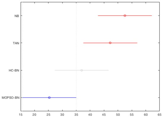
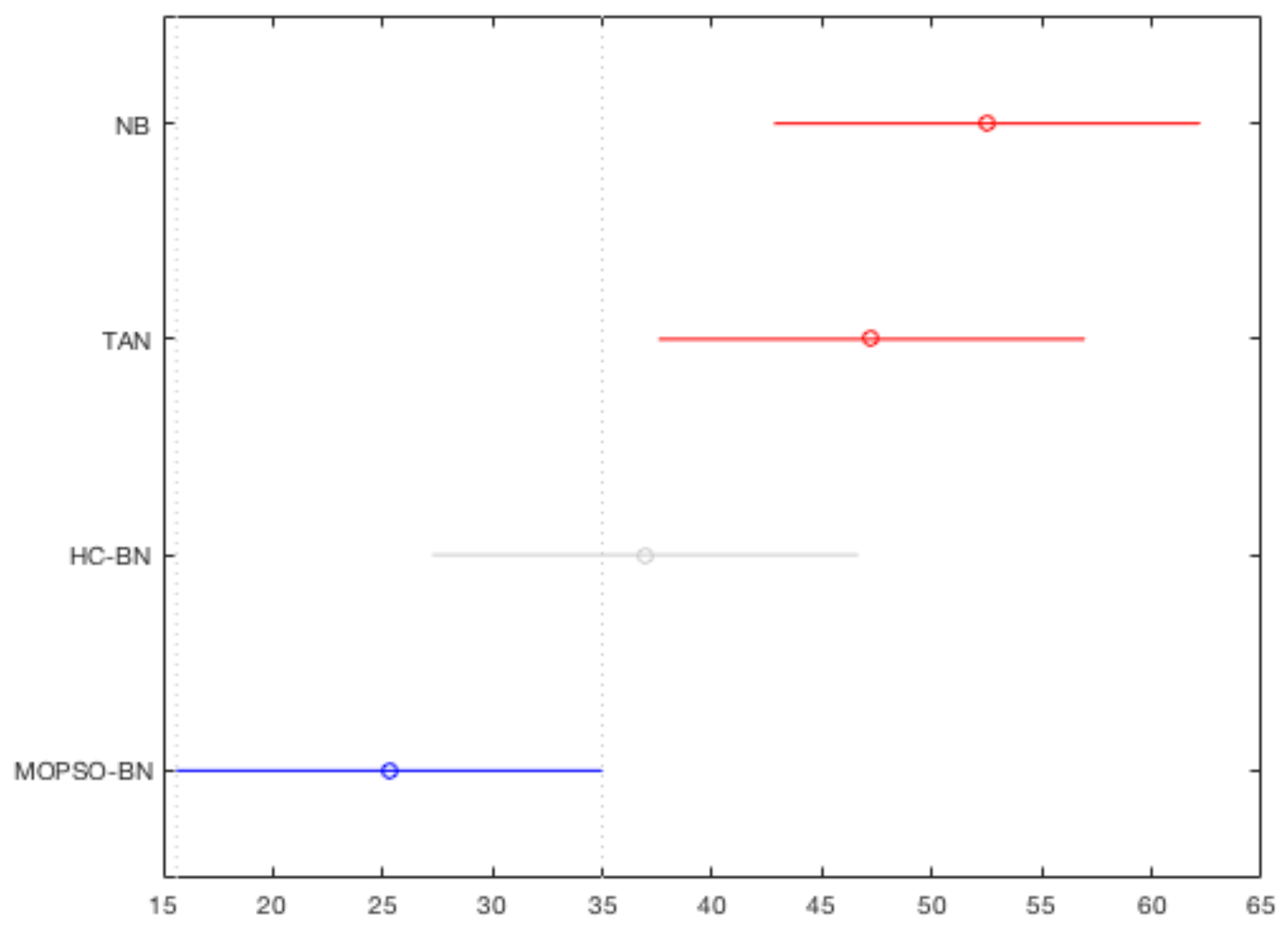
Table 4 shows misclassification and standard deviation of each algorithm (NB, TAN, HC-BN, and our chosen solution from the Pareto front). We highlight the classifier with the fewest misclassifications in boldface. To conduct a statistical comparison, we applied the non-parametric 95%-confidence Kruskal–Wallis multi-comparison test. According to this test, there is a significant difference between NB, TAN, HC-BN, and MOPSO-BN but none between MOPSO-BN and HC-BN. To further analyze those results and the statistical validation, we applied the post hoc Bonferroni test. Figure 7 shows the results, where it is possible to observe how our obtained solution has a better performance than TAN and NB. However, we see a similar performance between our proposed MOPSO-BN and HC-BN. Additionally, we applied the 95% non-parametric Mann–Whitney U test between HC-BN and MOPSO-BN; the results show our proposed approach outperforms others in 6 datasets, ties in 12 datasets, and has worse performance in just two datasets.

Figure 7. Post-hoc Bonferroni test to compare the performance of the four classifiers considering all datasets. The x-axis shows the confidence intervals of the midrange, and the y-axis shows the names of each classifier.

Results published by [16], where twenty-six datasets from UCI are tested, show that in 13 datasets TAN displays a significant difference between BNs using K2 and HC as the search procedure. Our results show better accuracy. Unfortunately, Madden’s results do not show the MDL metric for each model or the models learned, making it impossible to compare MDL. Similarly, the work of [52] shows poor accuracy when MDL is used as the driving metric. They propose a new score, risk minimization by cross-validation (RMVC), for an HC-based algorithm. One of their conclusions is that the best results are obtained when the initial structure is an NB rather than an empty network. Although EAs can learn robust structures compared with standard methods such as the K2 algorithm or simple deterministic methods, such as HC [58], the initialization of the search space can improve results [59]. MOPSO-BN employs random particle initialization, which helps the search process, but it is also possible to incorporate information about conditional independence between variables to further improve results. The work of [52] does not show the learned model using MDL; similarly, refs. [15,60] do not.

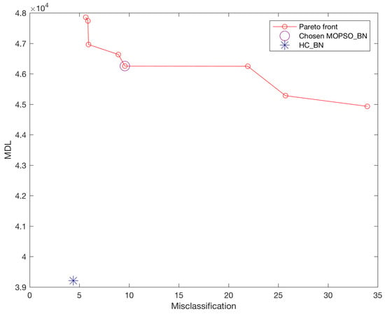
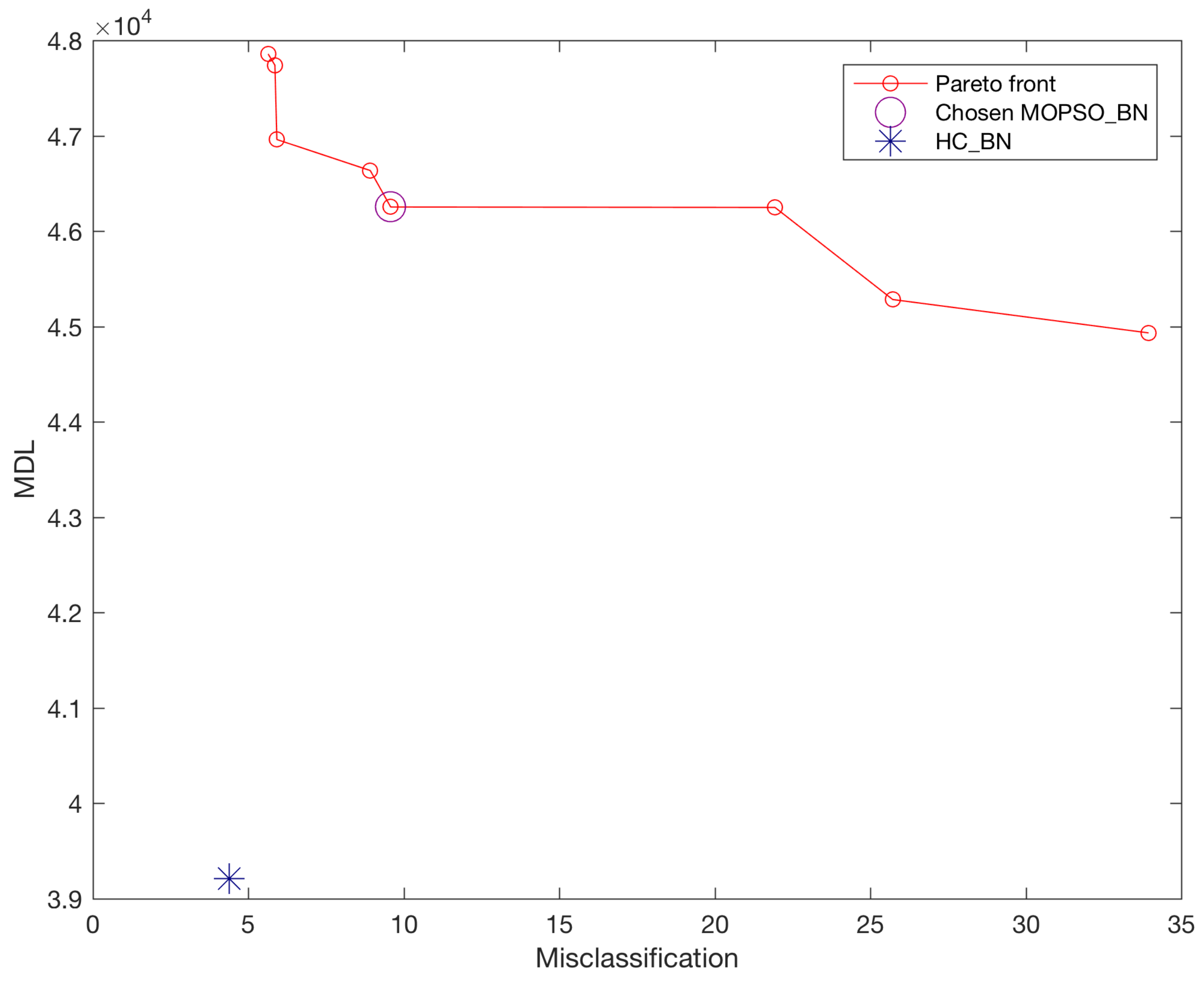
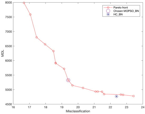
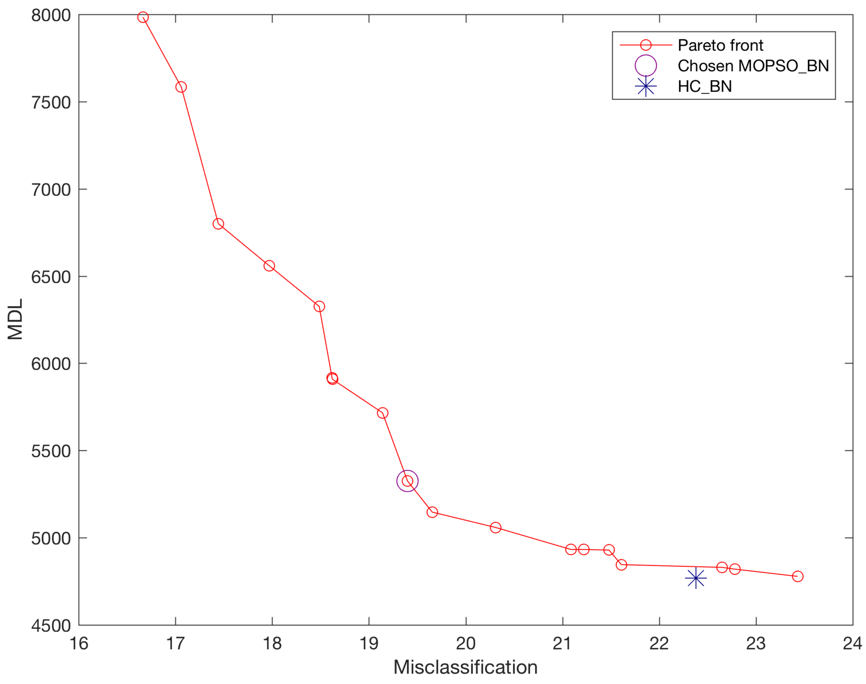
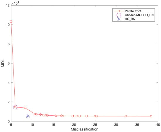
Table 4 shows that the chosen solution has the biggest value of MDL in 19 cases. These results agree with [8,15,52], who assert that a relatively good MDL score does not necessarily yield suitable classifiers. Note that we are empirically selecting an overall solution from a set of solutions and that we consider this solution to offer a good trade-off between misclassification and MDL, with the advantages that entail; nevertheless, our solution leaves open the possibility for expert input. Regarding Pareto fronts, they have advantages and have been used extensively before (see Figure 8, Figure 9 and Figure 10).

Figure 8. Accumulated Pareto front of Chess dataset obtained by ten runs of MOPSO-BN.

Figure 9. Accumulated Pareto front of Pima dataset obtained by ten runs of MOPSO-BN.

Figure 10. Accumulated Pareto front of Waveform dataset obtained by ten runs of MOPSO-BN.

3.4. Computational Cost Analysis

A natural concern when proposing a population-based metaheuristic such as MOPSO-BN is whether the additional computational investment over deterministic methods is justified by the gains in solution quality. In this section, we provide a theoretical analysis of the computational cost of each method and argue that the trade-off is favorable for MOPSO-BN in the context of BN structure learning for classification.

3.4.1. Cost of Deterministic Baseline Methods

The compared deterministic methods—NB, TAN, and HC-BN—have well-known computational properties. NB requires only a single pass over the data to estimate marginal and conditional frequency tables, with a cost of $O(N·n)$, where N is the number of instances and n is the number of variables. Its structural assumption (all attributes are conditionally independent, given the class) requires no search whatsoever. TAN augments NB by computing a maximum spanning tree over the $\left({\displaystyle \genfrac{}{}{0pt}{}{n}{2}}\right)$ pairwise conditional mutual information values, which adds a cost of $O(n^2·N)$ for the mutual information estimation and $O(n^{2}logn)$ for Prim’s or Kruskal’s algorithm [51]. Both methods are therefore extremely fast in practice, but they impose rigid structural constraints on the BN topology that severely limit their representational power: NB assumes no dependencies among attributes, and TAN allows at most one additional parent per attribute beyond the class node.

HC-BN performs a greedy local search in the space of DAGs, iteratively evaluating arc additions, deletions, and reversals and accepting those that improve the MDL score. Its cost per iteration is $O\left(n^2\right)$ score evaluations, each requiring $O(N·q_i·r_i)$ operations to update the sufficient statistics, where $q_i$ is the number of parent configurations of variable $X_i$ and $r_i$ is the number of its possible values. While HC-BN is significantly more flexible than NB and TAN in terms of the structures it can represent, it is a deterministic single-start greedy algorithm that is well known to be highly sensitive to the initial structure and prone to converging to local optima [58]. Its output is always a single network, providing no information about the landscape of alternative solutions or the trade-offs between competing objectives.

3.4.2. Cost of MOPSO-BN

The computational cost of MOPSO-BN is determined by four components that operate at each iteration:

• MDL evaluation ($f_1$): Given a candidate BN structure represented as an adjacency matrix, the parameters $\Theta$ are estimated using the simple estimator [24], which requires a single pass over the dataset to compute frequency tables. The MDL score is then computed according to Equation (1), with a cost of $O(N·{\sum }_{i=1}^n{q}_i·r_i)$ per particle.
• Misclassification evaluation ($f_2$): The misclassification rate is computed via $s=10$-fold cross-validation (Equation (2)), which requires training and testing the BN classifier s times. The dominant cost is $O(s·N·{\sum }_{i=1}^n{q}_i·r_i)$ per particle, making this the most expensive component of each evaluation.
• Cycle repair: The repair operator that ensures DAG validity operates directly on the adjacency matrix of each candidate BN and has a cost of $O\left(n^2\right)$ per particle. It handles three types of cycles: (i) self-cycles, detected by inspecting the diagonal of the adjacency matrix in $O\left(n\right)$ and resolved by setting the offending entry to 0; (ii) bi-directional cycles, detected by checking for simultaneous non-zero entries at positions $(i,j)$ and $(j,i)$ in $O\left(n^2\right)$ and resolved by randomly removing one of the two conflicting arcs; and (iii) general cycles of length greater than 2, identified by inspecting directed paths in the adjacency matrix and resolved by randomly removing one of the arcs responsible for closing the loop [28]. By applying this repair mechanism at each iteration, every candidate solution evaluated by MOPSO-BN is guaranteed to correspond to a valid DAG.
• Hypervolume contribution: The selection of $\overrightarrow{gbest}$ requires computing the hypervolume contribution ${\Delta }_h(s)$ of each solution in the archive A (Equation (5)). For a bi-objective problem, this can be computed exactly in $O\left(\right|A|log|A\left|\right)$ time, where $\left|A\right|$ is the archive size [40].

The total number of fitness evaluations per dataset is

$$E_{total}=R\times I\times P=10\times 200\times 100=\mathrm{200,000}$$

(9)

where $R=10$ is the number of independent runs, $I=200$ is the number of iterations per run, and $P=100$ is the swarm size. This represents a substantially larger computational investment than any of the deterministic baselines.

3.4.3. Justification of the Computational Trade-Off

Despite its higher computational cost, the investment in MOPSO-BN is justified on both theoretical and practical grounds.

Search Space Coverage

The number of possible DAG structures over n variables grows super-exponentially according to Robinson’s formula [3] (Equation (6)). For example, with $n=10$ variables, the number of possible DAGs exceeds $4\times {10}^{18}$, making any exhaustive evaluation completely infeasible. Deterministic methods such as HC-BN navigate this space via a single greedy trajectory, which is computationally cheap but sacrifices global search. In contrast, MOPSO-BN maintains a population of $P=100$ particles that simultaneously explore different regions of the DAG space, guided by both individual experience (pbest) and collective knowledge (gbest). This population-based mechanism provides a substantially broader coverage of the search space, reducing the risk of premature convergence to poor local optima—a well-documented limitation of greedy methods in combinatorial optimization problems [58].

Bi-Objective Optimization and Pareto Front

A fundamental limitation of all deterministic baselines is that they optimize a single objective and return a single solution. HC-BN, for instance, uses MDL as its scoring function and outputs the network with the smallest MDL value. As demonstrated graphically in Figure 4 and Figure 5 and quantitatively in Table 3, the network with the minimum MDL value is not necessarily the one with the best misclassification rate, and vice versa. This discrepancy is the central motivation of our bi-objective approach. MOPSO-BN simultaneously minimizes both $f_1$ (MDL) and $f_2$ (misclassification), producing a Pareto front of non-dominated solutions that explicitly trade off these two conflicting objectives. This output richness cannot be obtained by running NB, TAN, or HC-BN multiple times since these methods do not explore the objective space in a structured way. The additional computational cost of MOPSO-BN is therefore the price to be paid for obtaining this richer, more informative output.

Offline Learning Context

In the majority of practical applications of BNs—including medical diagnosis [2], fault detection, and risk assessment—the structure learning phase is performed offline, prior to deployment. Once the model is learned, inference is carried out online at negligible cost. In this context, the higher training cost of MOPSO-BN is a one-time investment that is amortized over the entire operational lifetime of the deployed model. Moreover, since MOPSO-BN returns a set of Pareto-optimal solutions rather than a single network, the end-user or domain expert can select the most appropriate model for a specific deployment scenario—for instance, prioritizing misclassification in safety-critical settings or MDL in resource-constrained environments—without the need to rerun the algorithm.

Comparison with HC-BN as the Closest Baseline

Among the compared methods, HC-BN is the most relevant computational baseline as it also performs search-based MDL optimization. The key difference is that HC-BN performs a single deterministic greedy trajectory, while MOPSO-BN runs 10 independent multi-objective searches with a population of 100 particles. Although this makes MOPSO-BN considerably more expensive, the Mann–Whitney U test results in Table 4 show that MOPSO-BN significantly outperforms HC-BN in 6 out of 20 datasets and achieves comparable performance in 12 others, with inferior results in only 2 datasets. Furthermore, the MDL values of the selected MOPSO-BN solution are higher than those of HC-BN in 19 out of 20 cases, confirming that MOPSO-BN deliberately trades a higher MDL value for a better misclassification rate—a behavior structurally impossible for HC-BN, which only optimizes MDL. This confirms that the additional computational cost of MOPSO-BN yields a qualitatively different, richer type of solution that single-objective deterministic methods cannot produce by construction.

Scalability Considerations

We acknowledge that the fixed budget of 200,000 function evaluations may become a limiting factor for datasets with a very large number of variables n since the cost of each evaluation grows with the complexity of the BN structure. For the 20 datasets used in our experiments, which range from 6 to 36 variables (Table 2), this budget was found to be sufficient to produce competitive Pareto fronts across all 10 independent runs, as evidenced by the consistency of the results shown in Figure 8, Figure 9 and Figure 10. For larger networks, strategies such as automatic algorithm configuration [61] or adaptive budget allocation could be used to dynamically adjust the number of evaluations based on network complexity, and are considered part of our future work.

3.5. Ablation Analysis

To clarify the individual contribution of each component of MOPSO-BN, we present a structured ablation analysis decomposing the proposed method into four configurations: (1) PSO-MDL, which uses PSO with only the MDL objective $f_1$; (2) PSO-Misc, which uses PSO with only the misclassification objective $f_2$; (3) MOPSO (no selection), which runs the full bi-objective search but selects a random solution from the Pareto front; and (4) MOPSO-BN (proposed), the complete method with reference-point preference handling. Table 5 summarizes the expected behavior of each configuration.

Table 5. Summary of the ablation analysis. Each configuration isolates one component of MOPSO-BN and its expected effect on MDL and misclassification performance.

Configuration	Objectives	Search	Selection	Expected Behavior
PSO-MDL	$f_1$ only	PSO	Best $f_1$	Low MDL but high misclassification risk, analogous to HC-BN
PSO-Misc	$f_2$ only	PSO	Best $f_2$	Low misclassification but high MDL, overfitting risk
MOPSO (no sel.)	$f_1+f_2$	MOPSO	Random	Pareto front available but inconsistent solution quality across runs
MOPSO-BN (proposed)	$f_1+f_2$	MOPSO	Ref. point	Balanced trade-off, competitive and reproducible on both objectives

The contribution of each component is supported by evidence already present in the paper. First, regarding the MDL objective: the exhaustive evaluation in Section 3.2 shows that the network with the minimum MDL value does not necessarily achieve the best misclassification rate (Table 3), with differences exceeding $100\%$ in MDL between the minimum-MDL and minimum-misclassification networks in datasets such as Balance Scale ($4573.73$ vs. $9599.58$). This directly demonstrates that PSO-MDL alone—like HC-BN—cannot guarantee good classification performance, motivating the inclusion of $f_2$. Second, regarding the misclassification objective: optimizing $f_2$ alone would remove the structural regularization provided by MDL, leading to unnecessarily complex networks that overfit the training data, as evidenced by the consistently high MDL values of the minimum-misclassification networks in Table 4.

Third, regarding the Pareto front: Figure 8, Figure 9 and Figure 10 show that the Pareto front spans a wide range of trade-off solutions that are collectively inaccessible to any single-objective method, including regions where MOPSO-BN significantly outperforms HC-BN in misclassification (e.g., Cleve, crx, German, Tic-tac-toe, and Vehicle in Table 4).

Finally, regarding the reference-point selection, the chosen solution achieves a higher MDL than HC-BN in 19 out of 20 datasets (Table 4), confirming that the selection strategy explicitly balances both objectives rather than minimizing either in isolation, a behavior that random selection cannot reproduce consistently. Taken together, these observations demonstrate that each component of MOPSO-BN plays a distinct, non-redundant role: the MDL objective regularizes the structure, the misclassification objective drives classification performance, the MOPSO framework enables simultaneous Pareto-based optimization, and the reference-point strategy ensures a principled, reproducible solution selection. We acknowledge that a full experimental ablation with separate algorithm runs for each configuration would provide additional quantitative evidence, and we consider this a valuable direction for future work.

4. Conclusions and Future Work

A BN is a powerful tool for representing relationships between variables; although there are methods for learning BNs from data, their value depends on the particular application. In some cases, it is possible to exploit only some of the advantages of BNs, as NB or TAN do. The path to better utilize these benefits (by leveraging classification and representational power) could be costly since the learning process exhibits exponential growth in the number of parameters. Our proposed method explores the problem of automatically learning BN structures using MDL and misclassification as scoring metrics. A set of trade-off solutions is obtained for each dataset; we choose the solution closest to the origin as the competitive solution. We compare this chosen solution with NB, TAN, and BNs learned using HC. From this comparison, we conclude that the chosen solution achieves competitive results, particularly with respect to the misclassification objective. It is important to note that one of the main advantages of this approach is the set of trade-off solutions; the selection of a model can ultimately be performed by a domain expert. Additional advantages include that our proposed method can be applied to datasets from different domains and extended to other models, such as Support Vector Machines (SVMs) and Neural Networks.

As future work, we propose exploring the automatic configuration of parameters and the number of evaluations. Also, we plan to study alternative solutions to reduce the computational cost of the algorithm and extend the evaluation framework to include class-sensitive metrics such as F1-score, Precision, Recall, and AUC, which provide a more complete characterization of classification performance in datasets with imbalanced class distributions. In particular, AUC represents a promising alternative second objective for the bi-objective framework, given its threshold-independence and its natural compatibility with the probabilistic outputs of Bayesian network classifiers. The whole set of our results can be found at the following link: https://sites.google.com/view/vaguilerar/thesis (accessed on 26 February 2026).

References

- Pearl, J. Bayesian networks: A model of self-activated memory for evidential reasoning. In Proceedings of the 7th Conference of the Cognitive Science Society, University of California, Irvine, CA, USA, 15–17 August 1985; pp. 329–334. [Google Scholar]
- Heckerman, D. A Tutorial on Learning with Bayesian Networks. In Learning in Graphical Models; Jordan, M.I., Ed.; MIT Press: Cambridge, MA, USA, 1999; pp. 301–354. [Google Scholar]
- Robinson, R.W. Counting unlabeled acyclic digraphs. In Combinatorial Mathematics V; Lecture Notes in Mathematics; Little, C., Ed.; Springer: Berlin/Heidelberg, Germany, 1977; Volume 622, Chapter 2; pp. 28–43. [Google Scholar] [CrossRef] [Scilit]
- Buntine, W. A Guide to the Literature on Learning Probabilistic Networks from Data. IEEE Trans. Knowl. Data Eng. 1996, 8, 195–210. [Google Scholar] [CrossRef] [Scilit]
- Neapolitan, R.E. Learning Bayesian Networks; Prentice-Hall, Inc.: Upper Saddle River, NJ, USA, 2003. [Google Scholar]
- Rónán, D.; Qiang, D.; Stuart, A. Learning Bayesian networks: Approaches and issues. Knowl. Eng. Rev. 2011, 26, 99–157. [Google Scholar] [CrossRef] [Scilit]
- Hansen, M.H.; Yu, B. Model Selection and the Principle of Minimum Description Length. J. Am. Stat. Assoc. 2001, 96, 746–774. [Google Scholar] [CrossRef] [Scilit]
- Friedman, J.H. On Bias, Variance, 0’/1 Loss, and the Curse-of-Dimensionality. Data Min. Knowl. Discov. 1997, 1, 55–77. [Google Scholar] [CrossRef] [Scilit]
- Cerquides, J.; Mántaras, R.L. TAN Classifiers Based on Decomposable Distributions. Mach. Learn. 2005, 59, 323–354. [Google Scholar] [CrossRef] [Scilit]
- Keogh, E.J.; Pazzani, M.J. Learning the structure of augmented Bayesian classifiers. Int. J. Artif. Intell. Tools 2002, 11, 587–601. [Google Scholar] [CrossRef] [Scilit]
- Hamine, V.; Helman, P. Learning optimal augmented Bayes networks. arXiv 2005, arXiv:cs/0509055. [Google Scholar] [CrossRef] [Scilit]
- Jing, Y.; Pavlovic, V.; Rehg, J.M. Efficient discriminative learning of Bayesian network classifier via boosted augmented naive Bayes. In Proceedings of the 22nd International Conference on Machine Learning (ICML-05); Raedt, L.D., Wrobel, S., Eds.; ACM: New York, NY, USA, 2005; pp. 369–376. [Google Scholar]
- Carvalho, A.M.; Oliveira, A.L.; Sagot, M.F. Efficient Learning of Bayesian Network Classifiers. In Proceedings of the AI 2007: Advances in Artificial Intelligence, Gold Coast, Australia, 2–6 December 2007; Springer: Berlin/Heidelberg, Germany, 2007; pp. 16–25. [Google Scholar] [CrossRef] [Scilit]
- Bouhamed, H.; Masmoudi, A.; Lecroq, T.; Rebai, A. A New Approach for Bayesian Classifier Learning Structure via K2 Algorithm. In Proceedings of the Emerging Intelligent Computing Technology and Applications, 8th International Conference, ICIC 2012, Huangshan, China, 25–29 July 2012; Communications in Computer and Information Science; Huang, D., Gupta, P., Zhang, X., Premaratne, P., Eds.; Springer: Berlin/Heidelberg, Germany, 2012; Volume 304, pp. 387–393. [Google Scholar] [CrossRef] [Scilit]
- Grossman, D.; Domingos, P. Learning Bayesian Network Classifiers by Maximizing Conditional Likelihood. In Proceedings of the Twenty-First International Conference on Machine Learning (ICML’04), New York, NY, USA, 4–8 July 2004; p. 46. [Google Scholar] [CrossRef] [Scilit]
- Madden, M.G. On the Classification Performance of TAN and General Bayesian Networks. In Research and Development in Intelligent Systems XXV; Bramer, M., Petridis, M., Coenen, F., Eds.; Springer: London, UK, 2009; pp. 3–16. [Google Scholar]
- Cooper, G.F.; Herskovits, E. A Bayesian Method for the Induction of Probabilistic Networks from Data. Mach. Learn. 1992, 9, 309–347. [Google Scholar] [CrossRef] [Scilit]
- Gheisari, S.; Meybodi, M.R.; Dehghan, M.; Ebadzadeh, M.M. Bayesian network structure training based on a game of learning automata. Int. J. Mach. Learn. Cybern. 2017, 8, 1093–1105. [Google Scholar] [CrossRef] [Scilit]
- Hastie, T.; Tibshirani, R.; Friedman, J. The Elements of Statistical Learning; Springer Series in Statistics; Springer: New York, NY, USA, 2001. [Google Scholar]
- Fang, W.; Zhang, W.; Ma, L.; Wu, Y.; Yan, K.; Lu, H.; Sun, J.; Wu, X.; Yuan, B. An efficient Bayesian network structure learning algorithm based on structural information. Swarm Evol. Comput. 2023, 76, 101224. [Google Scholar] [CrossRef] [Scilit]
- Blanco, R.; Inza, I.; Larrañaga, P. Learning Bayesian networks in the space of structures by estimation of distribution algorithms. Int. J. Intell. Syst. 2003, 18, 205–220. [Google Scholar] [CrossRef] [Scilit]
- Li, X.; He, X.; Chen, C. A Method for Learning Bayesian Networks by Using Immune Binary Particle Swarm Optimization. In Proceedings of the Database Theory and Application; Communications in Computer and Information Science; Slezak, D., Kim, T., Zhang, Y., Ma, J., Chung, K., Eds.; Springer: Berlin/Heidelberg, Germany, 2009; Volume 64, pp. 115–121. [Google Scholar] [CrossRef] [Scilit]
- Kuo, S.C.; Wang, H.J.; Wei, H.Y.; Chen, C.C.; Li, S.T. Applying MDL in PSO for learning Bayesian networks. In Proceedings of the 2011 IEEE International Conference on Fuzzy Systems (FUZZ-IEEE 2011), Taipei, Taiwan, 27–30 June 2011; pp. 1587–1592. [Google Scholar] [CrossRef] [Scilit]
- Hall, M.; Frank, E.; Holmes, G.; Pfahringer, B.; Reutemann, P.; Witten, I.H. The WEKA Data Mining Software: An Update. SIGKDD Explor. Newsl. 2009, 11, 10–18. [Google Scholar] [CrossRef] [Scilit]
- Li, G.; Xing, L.; Chen, Y. A New BN Structure Learning Mechanism Based on Decomposability of Scoring Functions. In Bio-Inspired Computing—Theories and Applications: 10th International Conference, BIC-TA 2015 Hefei, China, 25–28 September 2015, Proceedings; Springer: Berlin/Heidelberg, Germany, 2015; Chapter 19; pp. 212–224. [Google Scholar] [CrossRef] [Scilit]
- Wu, T.; Qian, H.; Liu, Z.; Zhou, J.; Zhou, A. Bi-objective evolutionary Bayesian network structure learning via skeleton constraint. Front. Comput. Sci. 2023, 17, 176350. [Google Scholar] [CrossRef] [Scilit]
- Aguilera-Rueda, V.J.; Cruz-Ramírez, N.; Mezura-Montes, E. Data-Driven Bayesian Network Learning: Towards a Bi-Objective Approach to Address the Bias-Variance Decomposition. Res. Comput. Sci. 2020, 149, 9–17. [Google Scholar]
- Aguilera-Rueda, V.J.; Cruz-Ramírez, N.; Mezura-Montes, E. Data-driven Bayesian Network learning: A bi-objective approach to address the bias-variance decomposition. Math. Comput. Appl. 2020, 25, 37. [Google Scholar] [CrossRef] [Scilit]
- Ross, B.J.; Zuviria, E. Evolving dynamic Bayesian networks with Multi-objective genetic algorithms. Appl. Intell. 2007, 26, 13–23. [Google Scholar] [CrossRef] [Scilit]
- Sun, B.; Zhang, X.; Jiang, J.; Gong, J.; Lin, D. Bayesian network structure learning by opposition-based learning. Sci. Rep. 2025, 15, 18447. [Google Scholar] [CrossRef] [Scilit]
- Fallahnejad, M.; Rezaeitabar, V.; Kazemi, M. Elastic net–based K2 algorithm for Bayesian network structure learning. Statistics 2025, 1–19. [Google Scholar] [CrossRef] [Scilit]
- Yang, W.T.; Tamssaouet, K.; Dauzere-Peres, S. Bayesian network structure learning using scatter search. Knowl.-Based Syst. 2024, 300, 112149. [Google Scholar] [CrossRef] [Scilit]
- He, C.; Wang, P.; Tian, L.; Di, R.; Wang, Z.; Yang, Y. A novel structure learning method of Bayesian networks based on the neighboring complete node ordering search. Neurocomputing 2024, 585, 127620. [Google Scholar] [CrossRef] [Scilit]
- Liu, H.; Liu, H.; Cai, Y.; Shi, Q.; Wang, N.; Zhang, L.; Li, S.; Cui, S. An improved Harris hawks optimization for Bayesian network structure learning via genetic operators. Soft Comput. 2023, 27, 14659–14672. [Google Scholar] [CrossRef] [Scilit]
- Wang, N.; Liu, H.; Zhang, L.; Cai, Y.; Shi, Q. An efficient skeleton learning approach-based hybrid algorithm for identifying Bayesian network structure. Eng. Appl. Artif. Intell. 2024, 133, 108105. [Google Scholar] [CrossRef] [Scilit]
- Dang, Y.; Gao, X.; Wang, Z. A Novel Hyper-Heuristic Algorithm for Bayesian Network Structure Learning Based on Feature Selection. Axioms 2025, 14, 538. [Google Scholar] [CrossRef] [Scilit]
- Yan, Y.; Zhang, Y.; Zhou, L.; Zhang, F.; Wang, H. Acoustic signals-based probabilistic fault diagnosis for expansion joints of small and medium bridges using Bayesian ensemble learning. Eng. Struct. 2026, 354, 122379. [Google Scholar] [CrossRef] [Scilit]
- Li, H.; Zhang, Y.; Wang, H.; Xu, Y.; Li, D. An explainable deep ensemble model for probabilistic prediction of typhoon effects on a long-span bridge. J. Wind Eng. Ind. Aerodyn. 2026, 269, 106330. [Google Scholar] [CrossRef] [Scilit]
- Engelbrecht, A.P. Fundamentals of Computational Swarm Intelligence; John Wiley & Sons: Hoboken, NJ, USA, 2006. [Google Scholar]
- Nebro, A.J.; Durillo, J.J.; García-Nieto, J.; Coello, C.A.; Luna, F.; Alba, E. SMPSO: A New PSO-based Metaheuristic for Multi-objective Optimization. In Proceedings of the 2009 IEEE Symposium on Computational Intelligence in Multicriteria Decision-Making (MCDM 2009); IEEE Press: New York, NY, USA, 2009; pp. 66–73. [Google Scholar]
- Nebro, A.J.; Durillo, J.J.; Coello, C.A. Analysis of leader selection strategies in a multi-objective Particle Swarm Optimizer. In Proceedings of the IEEE Congress on Evolutionary Computation, Cancun, Mexico, 20–23 June 2013; pp. 3153–3160. [Google Scholar]
- Kurgan, L.A.; Cios, K.J. CAIM discretization algorithm. IEEE Trans. Knowl. Data Eng. 2004, 16, 145–153. [Google Scholar] [CrossRef] [Scilit]
- Coello Coello, C.A.; Van Veldhuizen, D.A.; Lamont, G.B. Evolutionary Algorithms for Solving Multi-Objective Problems; Kluwer Academic Publishers: New York, NY, USA, 2002. [Google Scholar] [CrossRef] [Scilit]
- Deb, K.; Kalyanmoy, D. Multi-Objective Optimization Using Evolutionary Algorithms; John Wiley & Sons, Inc.: Hoboken, NJ, USA, 2001. [Google Scholar]
- Friedman, N.; Goldszmidt, M. Learning Bayesian Networks from Data; Morgan Kaufmann: Burlington, MA, USA, 1999. [Google Scholar]
- Grünwald, P.D. The Minimum Description Length Principle (Adaptive Computation and Machine Learning); The MIT Press: Cambridge, MA, USA, 2007. [Google Scholar]
- Cruz-Ramírez, N.; Acosta-Mesa, H.G.; Mezura-Montes, E.; Guerra-Hernández, A.; Hoyos-Rivera, G.d.J.; Barrientos-Martínez, R.E.; Gutiérrez-Fragoso, K.; Nava-Fernández, L.A.; González-Gaspar, P.; Novoa-del Toro, E.M.; et al. How good is crude MDL for solving the bias-variance dilemma? An empirical investigation based on Bayesian networks. PLoS ONE 2014, 9, e92866. [Google Scholar] [CrossRef] [Scilit]
- Teyssier, M. Ordering-based search: A simple and effective algorithm for learning Bayesian networks. In Proceedings of the UAI, Edinburgh, UK, 26–29 July 2005; pp. 584–590. [Google Scholar]
- Kelly, M.; Longjohn, R.; Nottingham, K. UCI Machine Learning Repository. 2023. Available online: https://archive.ics.uci.edu/ (accessed on 7 January 2025).
- Allen, T.V.; Greiner, R. Model Selection Criteria for Learning Belief Nets: An Empirical Comparison. In Proceedings of the International Conference on Machine Learning, Stanford, CA, USA, 29 June–2 July 2000; pp. 1047–1054. [Google Scholar]
- Friedman, N.; Geiger, D.; Goldszmidt, M.; Provan, G.; Langley, P.; Smyth, P. Bayesian Network Classifiers. Mach. Learn. 1997, 29, 131–163. [Google Scholar] [CrossRef] [Scilit]
- Kelner, R.; Lerner, B. Learning Bayesian network classifiers by risk minimization. Int. J. Approx. Reason. 2012, 53, 248–272. [Google Scholar] [CrossRef] [Scilit]
- Drugan, M.M.; Wiering, M.A. Feature selection for Bayesian network classifiers using the MDL-FS score. Int. J. Approx. Reason. 2010, 51, 695–717. [Google Scholar] [CrossRef] [Scilit]
- Shi, Y.; Eberhart, R. A modified particle swarm optimizer. In Proceedings of the 1998 IEEE International Conference on Evolutionary Computation Proceedings. IEEE World Congress on Computational Intelligence (Cat. No. 98TH8360), Anchorage, AK, USA, 4–9 May 1998; IEEE: New York, NY, USA, 1998; pp. 69–73. [Google Scholar] [CrossRef] [Scilit]
- Clerc, M.; Kennedy, J. The particle swarm—Explosion, stability, and convergence in a multidimensional complex space. IEEE Trans. Evol. Comput. 2002, 6, 58–73. [Google Scholar] [CrossRef] [Scilit]
- Fan, S.K.S.; Chang, J.M. A Modified Particle Swarm Optimizer Using an Adaptive Dynamic Weight Scheme. In Proceedings of the Digital Human Modeling; Duffy, V.G., Ed.; Spring: Berlin/Heidelberg, Germany, 2007; pp. 56–65. [Google Scholar]
- Gasse, M.; Aussem, A.; Elghazel, H. A hybrid algorithm for Bayesian network structure learning with application to multi-label learning. Expert Syst. Appl. 2014, 41, 6755–6772. [Google Scholar] [CrossRef] [Scilit]
- Larrañaga, P.; Karshenas, H.; Bielza, C.; Santana, R. A Review on Evolutionary Algorithms in Bayesian Network Learning and Inference Tasks. Inf. Sci. 2013, 233, 109–125. [Google Scholar] [CrossRef] [Scilit]
- Wong, M.L.; Leung, K.S. An efficient data mining method for learning Bayesian networks using an evolutionary algorithm-based hybrid approach. IEEE Trans. Evol. Comput. 2004, 8, 378–404. [Google Scholar] [CrossRef]
- Acid, S.; de Campos, L.M.; Castellano, J.G. Learning Bayesian Network Classifiers: Searching in a Space of Partially Directed Acyclic Graphs. Mach. Learn. 2005, 59, 213–235. [Google Scholar] [CrossRef] [Scilit]
- López-Ibáñez, M.; Dubois-Lacoste, J.; Pérez Cáceres, L.; Birattari, M.; Stützle, T. The irace package: Iterated racing for automatic algorithm configuration. Oper. Res. Perspect. 2016, 3, 43–58. [Google Scholar] [CrossRef] [Scilit]
Disclaimer/Publisher’s Note: The statements, opinions and data contained in all publications are solely those of the individual author(s) and contributor(s) and not of MDPI and/or the editor(s). MDPI and/or the editor(s) disclaim responsibility for any injury to people or property resulting from any ideas, methods, instructions or products referred to in the content. |
© 2026 by the authors. Licensee MDPI, Basel, Switzerland. This article is an open access article distributed under the terms and conditions of the Creative Commons Attribution (CC BY) license.