Fault Detection and Identification of Wind Turbines via Causal Spatio-Temporal Features and Variable-Level Normalized Flow

Abstract

Anomaly identification and fault localization of wind turbines through Supervisory Control and Data Acquisition (SCADA) data is a popular topic today, but most studies overlook the complex time-space interdependence between wind turbine (WT) SCADA variables, which results in low detection accuracy for anomalies in critical moving components of the wind turbine. To address this problem, this paper proposes a fault detection and identification method based on a dynamic graph model with a causal spatio-temporal attention mechanism and variable-level normalized flow. First, it introduces a spatio-temporal attention mechanism under causality to extract the spatio-temporal attention mechanism under causality to extract spatio-temporal features of the variables and uses a graph convolutional neural network to represent the extracted spatio-temporal features as a dynamic graph. Secondly, a dynamic normalization flow is suggested for calculating the logarithmic density estimation between variables. Finally, the anomaly scores are calculated through logarithmic density estimation. Based on these scores, anomalies are detected and localized. Experimental validation on real SCADA data from wind turbines demonstrates that the method can effectively identify abnormal operating states and provide early warnings, achieving higher accuracy and greater stability.

1. Introduction

Recently, driven by technological advancements and policy backing, the global wind power sector has witnessed rapid expansion. Presently, wind power generation technologies have reached a relatively mature stage, enabling large-scale commercial development at a comparatively lower cost [1]. Despite the rapid development of wind turbine equipment manufacturing technology, the operation and maintenance expenses caused by accidental failures and machine aging are still very high [2]. Therefore, to improve the reliability of wind turbines and prevent catastrophic events from occurring, it is necessary to improve the ability to recognize anomalies and diagnose faults in the critical moving parts of wind turbines.

Current techniques for wind turbine condition monitoring can be broadly categorized into wind turbine condition monitoring, which can be mainly categorized into two main categories: physical model-based and data-driven [3]. The physical model-based approach is mainly to construct physical or mathematical models of the wind turbine’s key moving parts and their related components. However, the construction of physical and mathematical models requires accurate model data, and when the system is more complex, the construction of the model requires a large amount of computation and a high level of professional knowledge [4]. Data-driven methods mainly include two categories of machine learning and deep learning, which are used to mine hidden information from a large amount of machine operation data and analyze the hidden information to obtain the machine’s operation status. Nowadays, most of the wind turbine equipment has a monitoring and data acquisition system (SCADA), which can obtain the state parameters of the machine operation, such as wind speed, temperature, rotational speed, environmental characteristics [5], and so on. Because the large amount of operating data it collects can be used for data-driven condition monitoring, the data-driven condition monitoring technique using SCADA as the data source has received a lot of attention from scholars. Machine learning methods mainly include support vector machines (SVMs) [6], Naive Bayes [7], and so on. However, machine learning has limited expression ability compared to deep learning models, is difficult to deal with complex nonlinear relationships, and has poor data migration and generalization ability.

Deep learning models exhibit strong representational capacity and excel at capturing complex nonlinear relationships, which can deal well with the complex nonlinear relationships among SCADA parameters [8]. Zhang et al. [9] proposed a new one-dimensional convolutional neural network fault diagnosis method using a batch normalization layer for better extraction of data features. Wang et al. [10] proposed a composite fault detection model that combines a three-dimensional squeezed excitation Convolutional Neural Network (3DSE-CNN) and a 2D Long Short-Term Memory Network (2DLSTM) composite fault detection model for wind turbines, which performs spatio-temporal feature extraction on SCADA data for fault diagnosis. Minh et al. [11] suggested a novel approach combining a one-dimensional convolutional neural network (1D CNN) with a bidirectional long and short-term memory network (Bi-LSTM), data reconstruction for enhanced structural health monitoring. Although existing deep learning approaches—such as LSTMs, GRUs, and spatio-temporal graph neural networks—effectively model temporal autocorrelation or spatial correlations among SCADA variables, they often adopt bidirectional or non-causal temporal dependencies, implicitly allowing future information to influence the representation of past states during training or inference. Moreover, although spatio-temporal interactions are increasingly modeled, the explicit integration of causal temporal constraints with learned spatial dependencies remains underexplored in the context of unsupervised wind turbine fault detection. This limitation can lead to unrealistic modeling assumptions and reduced reliability in real-time anomaly forecasting, where only past and present observations are available.

To solve these problems, many Scholars have performed spatio-temporal feature extraction of SCADA parameters and focused on the interdependence between the parameter nodes. Feng et al. [12] proposed a wind turbine root cause localization framework based on explicit-implicit knowledge fusion and multivariate time series graph neural networks, which fully utilizes the inter-variable dependency mining capability of graph structure learning and the time prediction advantage of time series graph neural networks. Zhu et al. [13] suggested a dynamic graph representation learning model based on a spatio-temporal self-attention mechanism, which can effectively learn the dynamics and interrelationships between variables for fault detection. The spatio-temporal characterization of SCADA variables can well discover the spatio-temporal interdependence between different variables and can respond to the abnormal state and faults of wind turbines in a more timely and accurate manner. Streser et al. [14] demonstrated the effectiveness of FMCW radar combined with 2D-CNNs for damage detection under fatigue loading, providing a robust non-contact monitoring solution. Rizk et al. [15] proposed an innovative approach that integrates hyperspectral imaging with a 3D Convolutional Neural Network (3D-CNN) for the detection of multiple damage types. This highlights the significant potential of 3D-CNNs in capturing complex spatial-spectral features for high-precision, image-based structural health monitoring.

Although many scholars conduct research on wind turbine condition monitoring, the current WT condition detection model still has the following problems: (1) Since SCADA contains various characteristic variables; the various variables are not correlation-free, the change of one variable will cause the change of multiple variables, and the correlation of these variables is often neglected in the anomaly detection, resulting in the reduction of the detection performance. (2) There is a complex spatio-temporal dependence between SCADA data variables, and many studies have not paid attention to their interdependence. (3) In SCADA variables, future data usually do not affect past data; however, in previous studies, no attention was paid to the dependencies between the front and back time steps, resulting in the flow of future information to the past. (4) Few of the multiple existing anomaly detection methods go further to provide root cause fault identification, but this is crucial for O&M and can save a lot of cost.

Aiming at the above problems given, this paper develops an unsupervised anomaly detection and identification framework by combining the dynamic graph representation of the causal spatio-temporal attention mechanism and the variable-level normalization process, which uses the causal attention mechanism with the help of causal masks to ensure that each time step can only pay attention to the time step before it when calculating the attention to efficiently capture causal dependency relationships in the data. At the same time, the dynamic graph convolutional neural network is combined to capture certain spatio-temporal correlations that may exist between different variables in the data, and the information between the nodes is aggregated through the adjacency matrix to extract the spatial features so that the model can consider the temporal and spatial changes at the same time. Secondly, the variable-level normalization process is designed to be able to model the distribution of each variable flexibly, simulate the density estimation of variables with the help of autoregression, and locate the faults of key motion subs of the wind turbine through density estimation. Finally, the validity of the proposed framework is verified by comparing it with a case study of a wind farm.

The main contributions of this paper are as follows:

• A causality-based spatio-temporal attention model is proposed, which can reasonably capture temporal causality and spatial features in SCADA data.
• A dynamic graph convolutional learning module is proposed, which is capable of feature fusion of the features obtained from the spatio-temporal attention mechanism, and can effectively reflect the dynamic spatio-temporal relationships of SCADA variables to realize anomaly detection.
• A variable-level normalization process and a framework for anomaly detection and fault identification are proposed to achieve density estimation of individual variables through the obtained spatio-temporal fusion features, so as to realize anomaly identification and fault localization of the key moving parts of wind turbines.

The next section of the paper is structured as follows: Section 2 gives the basic theoretical analysis, and Section 3 describes the proposed method in detail. Section 4 analyzes the experimental and comparative results, and Section 5 summarizes the conclusions.

2. Methodology

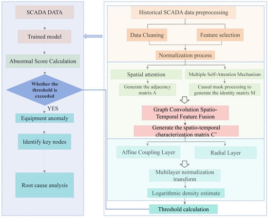
In this paper, we propose a framework for condition monitoring and fault diagnosis of wind turbine critical motion subsystems for wind turbines based on dynamic graph learning of causal spatio-temporal attention mechanism and variable-level normalized flow (CSDG-VNF). The basic model of the framework is shown in Figure 1.

Figure 1. The structure of the proposed CSDG-VNF model.

2.1. Data Preprocessing

In the training phase, firstly, the SCADA data should be preprocessed to remove the downtime data, abnormal state data, incomplete data, etc., from the data, and the missing data should be processed. At the same time, it is necessary to select the data in the data that are highly relevant to the fault diagnosis of the wind turbine’s key moving components, so that it can have better diagnostic results [16]. Then, the data are normalized to eliminate the influence of different data input ranges on the data weights.

2.2. Dynamic Graphical Representation of Spatio-Temporal Attention Mechanisms Under Causality

It should be noted that the term “causal” used in this paper refers specifically to temporal directionality in time-series modeling—i.e., ensuring that predictions at any time step depend only on past and present observations, not future ones. Our framework does not aim to infer true physical cause-and-effect relationships among SCADA variables, but rather to enforce temporal consistency for realistic and deployable anomaly forecasting.

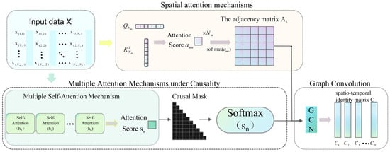
To construct a dynamic graph model with a spatio-temporal attention mechanism under causality, first, the data undergoes a spatial attention mechanism and a causal attention mechanism, respectively, to generate an adjacency matrix with spatial features and causality parameters with temporal features. These features are then fused via a graph convolutional neural network to capture the complex dependencies between variables in time series data to obtain spatio-temporal features, as shown in Figure 2.

Figure 2. Structure of spatio-temporal feature fusion method.

2.3. Anomaly Threshold Design Under Variable-Level Normalization

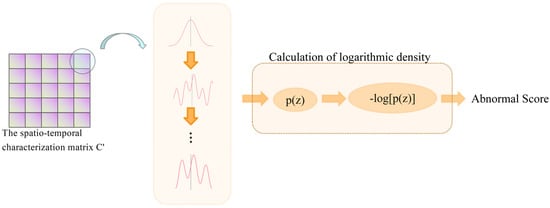
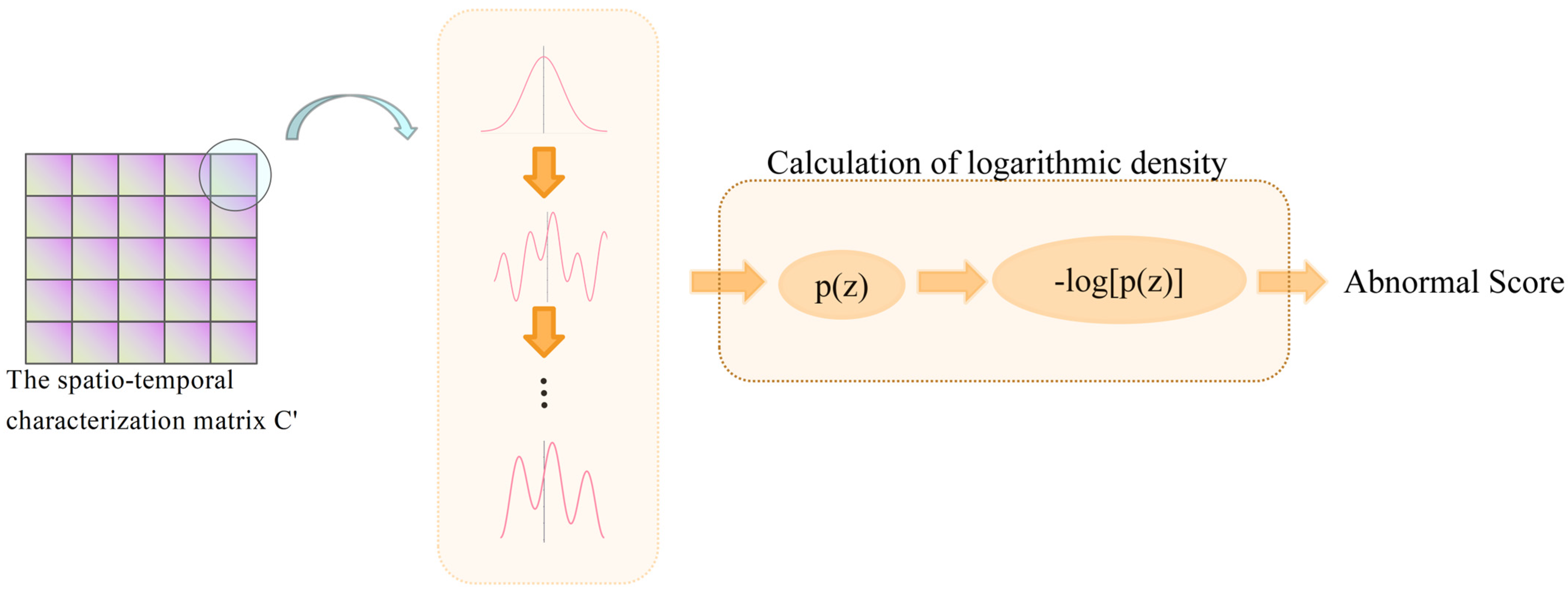
To design a variable-level normalized streaming framework that implements discriminative density estimation for individual variables while exploiting conditional information in dynamic spatio-temporal representations. The proposed method transforms complex, high-dimensional SCADA data distributions into easy-to-handle normalized Gaussian distributions through a series of invertible transformations, enabling accurate density estimation for anomaly detection, while the anomaly threshold can be set by the calculated probability density, as shown in Figure 3.

Figure 3. Variable-level normalized flow structure.

Unlike conventional multivariate normalizing flows that model the joint distribution of all variables simultaneously, a variable-level normalized flow treats each dimension (i.e., each SCADA variable) as a conditionally independent component whose transformation parameters are modulated by shared spatio-temporal context. Formally, given an input vector $x={[x_1,x_2,x_3,\dots x_D]}^T\in R^D$, the flow learns a set of invertible mappings $f_d(\cdot ;{\theta }_d(c))$ for each variable $x_d$, where $c\in R^{D^{\prime }}$ denotes the spatio-temporal feature representation (e.g., output from the graph convolution module) that serves as conditional context. This design enables flexible, per-variable density estimation while leveraging global dependencies through the conditioning signal, thereby balancing model expressiveness and computational efficiency.

2.4. Abnormality Monitoring and Fault Identification

Fault detection can be achieved by calculating the anomaly score from the resulting density estimates and comparing it with a set threshold. When an anomaly occurs, fault localization is achieved by identifying the critical nodes based on the log density of each variable. The function considers these nodes as possible sources of faults by taking the smallest log density variable at each time step as the critical node.

3. Detailed Design of the Model

3.1. Mechanisms of Spatio-Temporal Self-Attention Under Causality

In SCADA, there are interdependencies between variables. When an abnormality occurs in the key moving components of a wind turbine, there are usually multiple variables changing at the same time. Therefore, a spatial self-attention mechanism is used to capture the complex dependencies among variables in time series data. For each pair of features $(x_i,x_j)$, obtain their time series $x_{s_m}{x}_{s_n}$, where s represents each time step, while m and n represent the indices of the feature pair. The query vector Q, the key vector K and the scaling factor $d_k$ are then computed as follows: $Q=X_{s_m}·W_Q,K=X_{s_n}·W_K,d_k=\sqrt{N_t}$, Calculate the attention score $e_{s_{mn}}$ from the query vector $Q$ and the key vector $K$:

$$e_{s_{mn}}={\displaystyle \frac{Q·K^T}{d_k}},$$

(1)

Attention scores were normalized using the Softmax function to obtain $a_{s_{mn}}$:

$$a_{s_{mn}}=\mathrm{softmax}(e_{s_{mn}})={\displaystyle \frac{\exp (e_{s_{mn}})}{{\displaystyle {\sum }_{k=1}^n{e}_{s_{mn}}}}}.$$

(2)

Each attention score calculated is the spatial dependency between the parameter nodes, and the calculated attention scores are stored one by one in the attention matrix A_s. Adjacency matrix construction for graph convolution. In this work, the spatial attention weight matrix obtained in Equation (2) is directly used as the adjacency matrix for graph convolution. Specifically, given the spatial score matrix in Equation (1), we apply a row-wise Softmax:

$$A_{ij}={\displaystyle \frac{\exp (S_{IJ})}{{\displaystyle {\sum }_{K=1}^D\exp (S_{ij})}}}$$

(3)

where $D$ is the number of SCADA variables (nodes). Thus, $A\in R^{D\times D}$ defines a dense, directed, weighted graph in which all node pairs are connected, and the edge weight represents the attention-based dependency strength. We do not apply hard thresholding or a fixed top-k neighbor selection; the attention weights provide “soft connectivity” and satisfy ${\displaystyle {\sum }_j{A}_{ij}=1}$. The diagonal entries $A_{ii}$ naturally act as self-connections.

Meanwhile, the parameters of SCADA have a strict time series order, future data cannot influence past decisions, and system failure usually manifests itself as a chain reaction in the time series, so the temporal features of the input data are extracted using a multiple self-attention mechanism under causality. Get input sequence $X\in R^{B\times T\times D}$, where B is the input data batch size, T is the number of time steps, D is the feature dimension, the number of attention heads is set to H, and each head dimension satisfies $d_k=D/H$. The query vector Q, the key vector K, and the value vector V map the input X by a linear transformation to: $Q=X_{s_m}·W_Q,K=X_{s_n}·W_K,d_k=\sqrt{N_t}$. In the multi-head attention mechanism computation, Q, K, V are partitioned into H heads: $Q=[Q_1,Q_2,Q_3,\dots Q_H]$; K and V are identical. To ensure causality, a Causal Mask needs to be introduced to restrict the current time step to focus only on past time steps. The specific steps are as follows. Since the dimensionality of the data in the following section is 78, and to ensure it is divisible by the number of attention heads H, and considering that in classification tasks the number of heads is commonly set between 4 and 8, we choose H = 6 [16]. The full list and definitions of these 78 variables are available in the Supplementary Materials.

Calculate the attention mechanism score:

$$S_i={\displaystyle \frac{Q_i·{K_i}^T}{d_k}}.$$

(4)

To introduce causality, construct the lower triangular matrix M as a masking mechanism:

$$M_{ts}=\left\{\begin{array}{l}0, t\ge s\\ -\infty , t<s\end{array}\right..$$

(5)

Applying this to the score matrix makes the matrix focus only on past time steps:

$${S_i}^{\prime }=S_i\otimes M.$$

(6)

Apply Softmax function to the masked score matrix: $A_i=\mathrm{softmax}({S_i}^{\prime })$. When $t>s$, ${S_i}^{\prime }=-\infty$, $\mathrm{softmax}(-\infty )=0$, future time steps are masked. Then for each head $i$, the attention weight aggregation matrix is used:

$$h_i=A_i{V}_i.$$

(7)

The output of all heads is spliced and projected back to the original dimension D through the linear layer W^O to get the multi-head attention output matrix M:

$$M=MultiHead(Q,K,V)=Concat(h_1,h_2,h_3,\cdots ,h_H)W^O.$$

(8)

3.2. Graph Convolutional Neural Network Spatio-Temporal Feature Fusion

Let $A\in R^{D\times D}$ denote the attention-based spatial adjacency matrix learned in Equation (2). Since Equation (2) applies row-wise Softmax, $A$ is already normalized $({\displaystyle {\sum }_j{A}_{ij}=1})$; therefore, we directly use $A$ as the normalized adjacency in the graph convolution for spatial propagation.

$$S{P}_t=\widehat{A}{M}_t\in R^{N\times D}$$

(9)

Stack over t to $SP\in R^{T\times N\times D}$. Fuse with a linear layer and nonlinearity. The second and third dimensions of $S_p$ are transposed to obtain the spatial feature array $S_p^{\prime }$, of shape (B, T, D), through the designed graph-convolution linear layer for spatio-temporal feature fusion and ReLU activation function for nonlinear transformation:

$$C=\mathrm{Re}LU(L_1(A_s·S_p^{\prime })+L_2(S_p^{\prime }).$$

(10)

Transformation of the fused spatio-temporal feature matrix C using the linear layer $L_3$:

$$C^{\prime }=L_3(C).$$

(11)

where $L_1,L_2,L_3$ are all learnable fully connected layers, containing weight matrices and bias vectors; these parameters are automatically learned during training.

3.3. Variable-Level Normalization and Log-Density Computation

A normalizing flow consists of a sequence of invertible transformations. $f_1,f_2,\cdots ,f_k$ combinations. Transform a simple probability distribution, p_z(x), into a complex target distribution $p_x(x)=f_k·f_{k-1}·\cdots ·f_1(z)$.

A variable-level normalized flow, as employed in this work, does not assume statistical independence among SCADA variables. Instead, it models the conditional distribution of each variable given a shared spatio-temporal context. Specifically, the transformation parameters for each dimension are dynamically modulated by the fused spatio-temporal features (e.g., output from the graph convolution module), which encode inter-variable dependencies and temporal dynamics. This allows the flow to capture complex marginal behaviors of individual variables while implicitly accounting for their mutual correlations through the conditioning signal.

SCADA data contains multiple variables, and the computational complexity increases significantly as the number of variables increases significantly. The variable-level normalized flow can well integrate the spatio-temporal features obtained from SCADA data after processing as conditional information, and the sharing of parameters among variables reduces the model complexity while maintaining the expressive power. In this paper, the principles and steps of designing variable-level normalized flow are as follows. Affine Coupling Layer: the input x is divided into two parts $x_1$, $x_2$; one part passes through directly, and the other part is transformed by the neural network.

$$\left\{\begin{array}{l}{y}_1=x_1\\ y_2=x_2\odot \exp (s(x_1,C^{\prime })+t(x_1,C^{\prime })\end{array}\right..$$

(12)

where s and t are scale and offset parameters generated by the neural network and $C^{\prime }$ is the output of the graph convolutional network as conditional information. The logarithm of the Jacobi determinant is:

$$\log \det J_a={\displaystyle {\sum }_{i=1}^{D/2}{s}_i}.$$

(13)

D is the vector dimension and $s_i$ is the logarithmic scaling factor of the ith dimension.

The radial transform layer is a nonlinear transform that is realized by the following equation:

$$y=x+\beta ·{\displaystyle \frac{\alpha }{\left|x-x_0\right|+\alpha }}·(x-x_0).$$

(14)

where $x_0$ is the transformation center, α > 0 is a learnable scale parameter, and β ∈ R is a learnable intensity parameter. The logarithm of the Jacobi determinant is:

$$\log \left|\det J_r\right|=(d-1)\log \left|1+{\displaystyle \frac{\beta }{\alpha +r}}\right|+\log \left|1+{\displaystyle \frac{\beta \alpha }{{(\alpha +r)}^2}}\right|.$$

(15)

where d is the data dimension, $r=\left|x-x_0\right|$.

The above two transformation layers are designed as transformation blocks f, and the “multiple transformation layer combination” is realized by the way of “block stacking”. The variable-level normalizing flow stacks the above transformation blocks to form a complex invertible mapping to form a complex invertible transformation and the spatio-temporal features obtained above. The spatio-temporal feature matrix R obtained above is input to the variable-level normalization flow, which helps the normalization flow to estimate the conditional probability density of the data more accurately:

$$z=f_k·f_{k-1}·\cdots ·f_1(x).$$

(16)

3.4. Calculation of Log Densities and Anomaly Scores

After all the transformation blocks, the final latent variable z, according to the variable transformation formula, the probability density of z is:

$$p(z)=p(x)\times {{\displaystyle {\prod }_{k=1}^k\left|\det (\frac{\partial f_k}{\partial z_{k-1}})\right|}}^{-1}.$$

(17)

The logarithmic density of the input data x is:

$$\log p(x)=\log p(z)+{\displaystyle \sum _{k=1}^K\log \det J_k},$$

(18)

where $J_k$ is the Jacobi matrix of the kth transformation layer.

The log density is used to measure the probability that a data point is under a normal distribution. Under normal conditions, data points should have higher log densities because they are more consistent with the normal patterns learned by the model. When anomalous data are present, their log densities are significantly lower because they deviate from the normal distribution. By calculating the logarithmic density, the data points can be mapped to a numerical space, which facilitates the calculation of anomaly scores and the detection of anomalies. The anomaly scores are obtained by negatively averaging the log densities.

$$A{S}_i=-{\displaystyle \frac{1}{D}}{\displaystyle \sum _{d=1}^D\log (x_{(i,d)})}.$$

(19)

$x_{(i,d)}$ denotes the $d_{th}$ feature dimension of the $i_{th}$ sample. The lower the log density, the higher the anomaly score, indicating that the data points are more likely to be anomalous.

3.5. Anomaly Identification and Fault Localization

In this paper, the quartile method is used to calculate the 25th percentile (Q₁) and the 75th percentile (Q₃) of the anomaly score, and then the interquartile range (IQR = Q₃ − Q₁) is calculated. The threshold is then:

$$threshold=Q_3+\alpha \times IQR.$$

(20)

α is the scaling factor, set to 2. To evaluate the robustness of the IQR-based anomaly thresholding, we conduct a sensitivity analysis by varying the scaling factor α ∈ {1.0, 1.5, 2.0, 2.5, 3.0}.

Results indicate that the performance remains stable for α ∈ [1.5, 2.5]. This justifies our choice of α = 2 as a balanced trade-off between detection sensitivity and false alarms.

The design of the threshold is a critical step in fault detection, which is used to distinguish between normal and abnormal data. When the anomaly score exceeds the threshold value, it proves that the device is in an abnormal state.

Fault localization is done by comparing the log densities of each variable to find the most anomalous variable:

$$key\_nod{e}_{i,t}=\arg {\min }_{d=1}^D\log p(x_{i,t,d}),$$

(21)

$i$ denotes the sample index, t denotes the time step index, d denotes the variable dimension index, D denotes the total number of variables, and $\log p(x_{i,t,d})$ denotes the logarithmic density of variable d at time step t. $key\_nod{e}_{i,t}$ is the key node index of the $i_{th}$ sample.

Calculate the relative change in the adjacency matrix for normal and abnormal conditions:

$$c{g}_{i,j}={\displaystyle \frac{\left|A_{i,j}^{normal}-A_{i,j}^{abnormal}\right|}{A_{i,j}^{normal}+\xi }},$$

(22)

where $A_{i,j}^{normal}$ and $A_{i,j}^{abnormal}$ are the adjacency matrices in normal and abnormal states, respectively, $\xi$ is a small constant avoiding a zero denominator. Calculate the deviation index of other nodes based on key_node:

$$deviation\_inde{x}_j=c{g}_{k,j}, j=1,2,3\dots ,D.$$

(23)

Root cause determination:

$$root\_node=\arg {\max }_{j=1}^{D}deviation\_inde{x}_j.$$

(24)

4. Experimental Verification

In this paper, a wind farm in China with a rated parameter of 2 mw is used as an experimental case to validate the proposed method. The wind turbine SCADA fault records are shown in the following Table 1.

Table 1. Detailed fault information for the WT used in this study.

WT Number	SCADA First Alarm	SCADA Second Alarm		SCADA First Alarm Time	SCADA Second Alarm Time	SCADA First Reset Time	SCADA Second Reset Time
28	Generator winding and magnet temperature difference lead to large failure		Hydraulic oil temperature is too high		17:19 22 May 2022	21:58 22 May 2022	17:31 22 May 2022	22:01 22 May 2022

Among all subsystems, failures in the critical moving components result in the longest downtime per incident for a single failure, resulting in a great economic loss [17]. Moreover, the wind turbine critical motion subsystems are installed in high and narrow spaces, with great operation and maintenance costs [18]. Therefore, anomaly monitoring and fault identification of wind turbine key moving parts using SCADA data become key to research content.

The operation state of the key moving components of the wind turbine has a great relationship with the ambient temperature, humidity, wind speed, wind speed can directly affect the wind turbine gear box, main shaft, such as speed, torque, temperature, output power, but also can indirectly affect the gear box, main shaft lubricating oil and the temperature of the cooling water, the change of the output power at the same time also implies that the temperature of the stator of the windings change. Therefore, this paper selects the parameters related to the operation state of the key motion sub of the wind turbine as input features. And the SCADA selected parameter data are preprocessed [19].

4.1. Case Study and Experimental Effect Verification

Implementation details and training settings. The proposed model was implemented using the PyTorch 2.0.1 deep learning framework and trained on a Windows 10 workstation equipped with an NVIDIA GeForce RTX 4060 GPU with 8 GB memory (CUDA 12.6). Unless otherwise specified, the model was trained for 300 epochs with batch size B = 8 using the Adam optimizer with an initial learning rate of 0.01. A ReduceLROnPlateau learning-rate scheduler was used: the learning rate is multiplied by 0.5 if the training loss does not improve for 5 consecutive epochs. The training objective is to minimize the negative log-density (negative log-likelihood) output by the model.

The training data used in this paper is the SCADA data of wind turbine No. 28 from March to April 2022, which is collected every minute, with a total of 89,284 time steps, and the test set used is SCADA from 20:00 21 May 2022 to 15:00 24 May 2022 with a total of 4000 time steps. Where the SCADA data indicated that wind turbine No. 28 had a large generator winding and magnet temperature difference failure, and a large generator winding and magnet temperature difference failure at 17:19 on 22 May 2022 (time step 1281). A high hydraulic oil temperature warning occurred at 21:58:01 on 22 May 2022 (time step 1560), as shown in Table 2.

Table 2. Details of the No.28 WT dataset.

Dataset	Operational Time	Time Steps
Training set	From March to April 2022	89,284
Test set	From 20:00 21 May 2022 to 15:00 24 May 2022	4000
Failure occurrence time	17:19 on 22 May 2022, 21:58:01 on 22 May 2022	1281, 1560

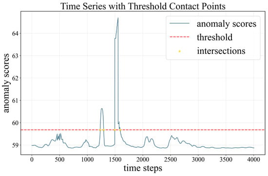
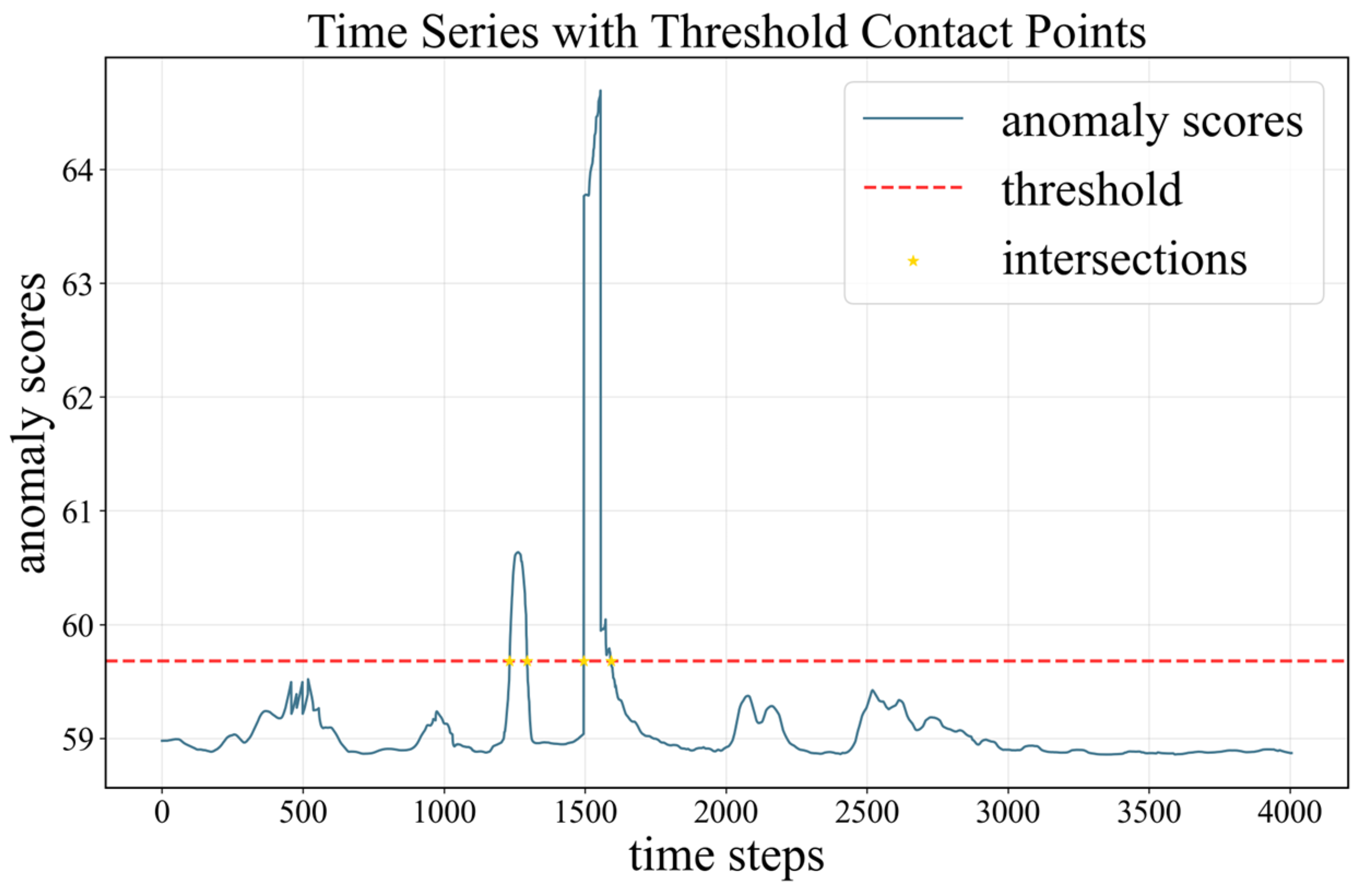
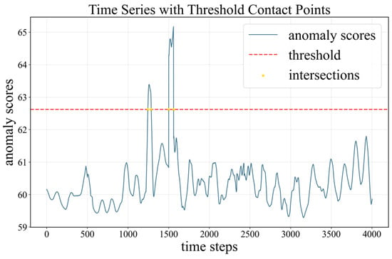
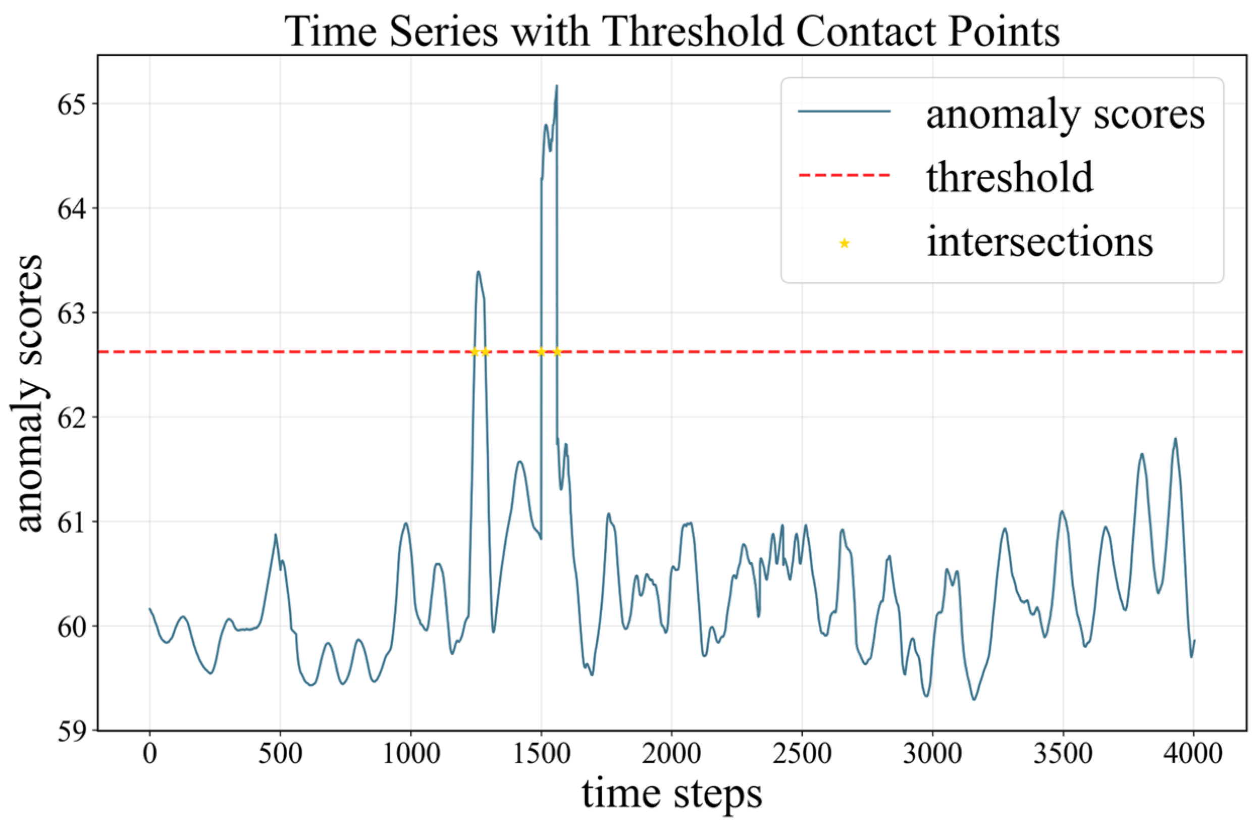
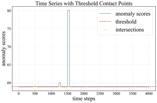
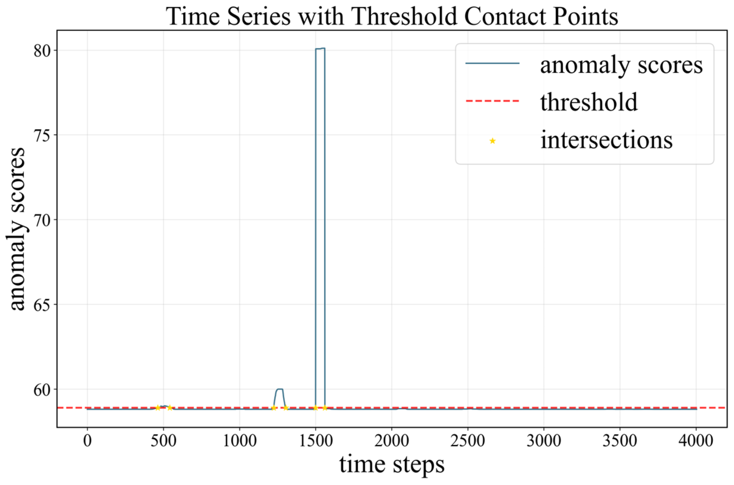
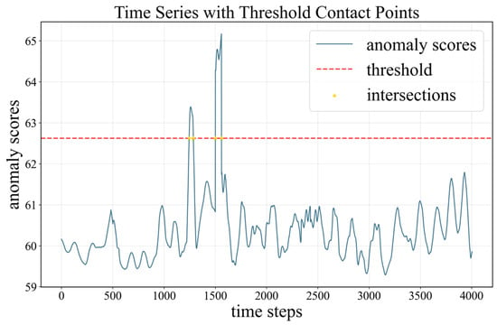
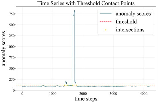
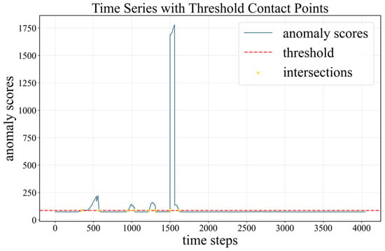
In this paper, the anomaly score is calculated by logarithmic density. When the anomaly score is elevated, it represents that the data deviates from the normal data, and when it exceeds the threshold value, the anomalous state is monitored. Figure 4, Figure 5 and Figure 6 show the comparison of the experimental results of the method proposed in this paper and the other two methods.

Figure 4. Calculated anomaly scores of the No.28 WT by proposed CSDG-VNF.

Figure 5. Calculated anomaly scores of the No.28 WT by proposed DG-VNF.

Figure 6. Calculated anomaly scores of the No.28 WT by proposed LSTM-CNN.

Figure 4 is measured by this experimental method, the anomaly fraction curve is found to be anomalous at time steps 1231 to 1296 and 1495 to 1597, and the wind turbine anomalous condition is found at 16:29 min on 22 May 2022 to 17:24 min on 22 May 2022 and at 20:53 min on 22 May 2022 to 22:35 min on 22 May 2022, and 28 wind turbine SCADA issued a warning of generator winding and magnet temperature difference failure at 17:19 on 22 May 2022 (time step 1281), which the model warned fifty minutes ahead of time, and SCADA issued a warning of high hydraulic oil temperature at 21:58 on 22 May 2022, which the model warned one hour and five minutes ahead of time.

Figure 5 shows the DG-VNF [20] anomaly score curve graph, the anomaly score curve found anomalies at time steps 1244 to 1286 and 1500 to 1560, and the model found at 16:42 on 22 May 2022 to 17:24 on 22 May 2022 and 20:58 on 22 May 2022 to 21:58 on 22 May 2022 wind turbine anomalous condition, 37 min and 1 h ahead of the SCADA warning, respectively.

Figure 6 shows the LSTM-CNN [21] anomaly score curves, the anomaly curves are found at time steps 444 to 562, 1223 to 1306, and 1500 to 1560, and the model’s results on 22 May 2022 at 3:22 min to 22 May 2022 at 5:20 min, 22 May 2022 at 16:21 min to 22 May 2022 at 17:44 min on 22 May 2022, and 20:58 min on 22 May 2022, and 21:58 min on 22 May 2022, when the wind turbine anomalous condition was detected, with the time steps 444 to 562 being misclassified, and the latter two being 58 min and 1 h ahead, respectively.

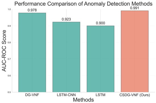
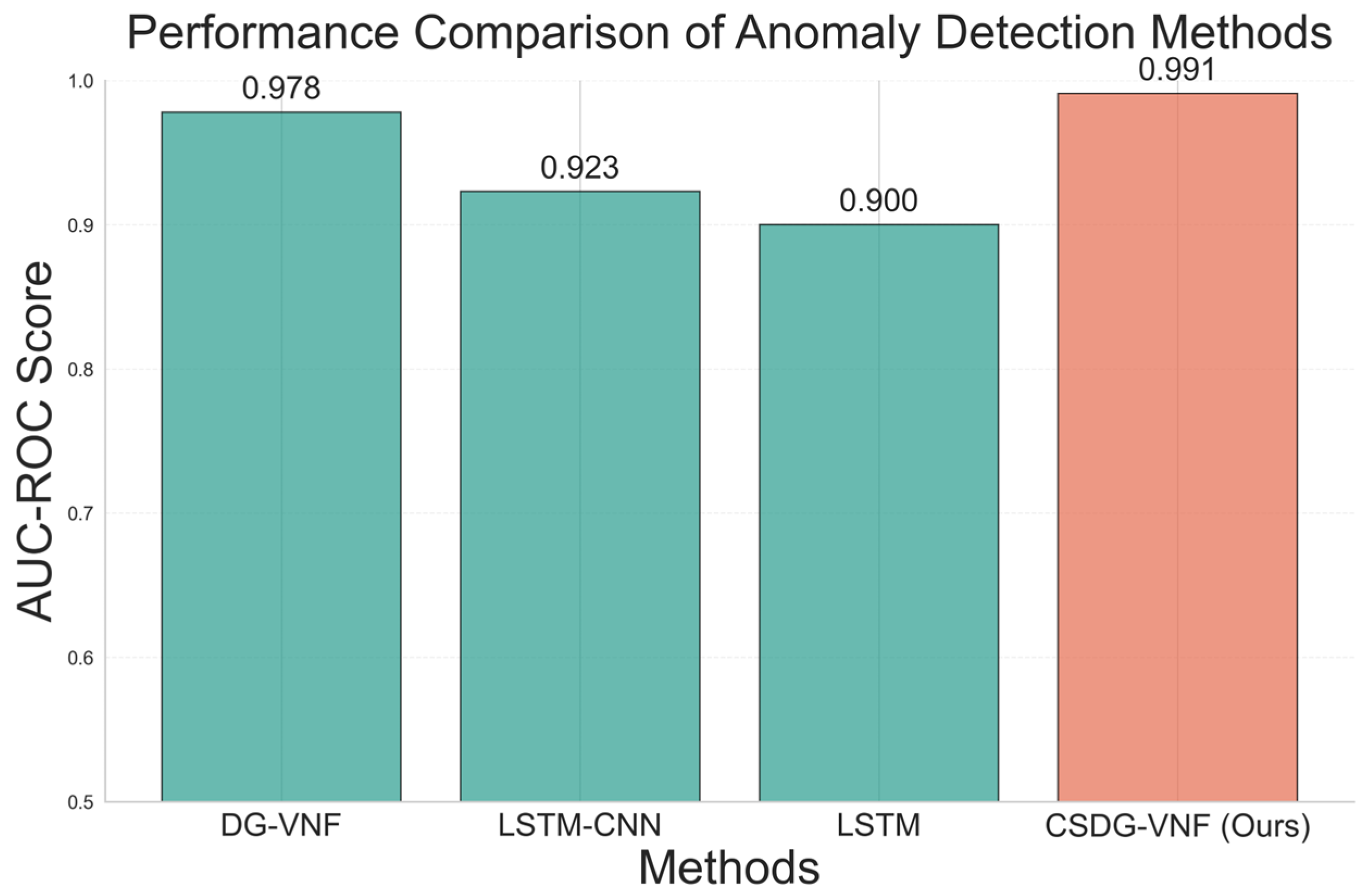
The experimental validation of the three experiments is shown in Figure 7. The experiments show that the proposed method is able to obtain stable spatio-temporal fusion variables by capturing the spatio-temporal feature dependencies among the variables and performs an accurate density estimation for anomaly detection after a variable-level normalized flow. The anomalous state can be recognized earlier compared to DG-VNF and has better stability without misclassification compared to LSTM-CNN.

Figure 7. Performance comparison of anomaly detection methods.

To further verify the experimental efficacy of the proposed method, the proposed method is compared with three methods: DG-VNF, LSTM-CNN, and LSTM for AUC (Area Under Curve) metrics [22]. In anomaly detection, the ROC curve and AUC are important indicators to evaluate the performance of the model. AUC refers to the area under the ROC curve, which is used to measure the performance of the binary classification model.

$$TPR={\displaystyle \frac{TP}{(TP+FN)}},$$

(25)

$$FPR={\displaystyle \frac{FP}{FP+TN}}.$$

(26)

where TP stands for true positives, and FP means false positives.

DG-VNF is a proposed dynamic graph representation learning and variable-level normalization flow based on self-attention, focusing on dynamic spatio-temporal correlation between variables, achieving fine density estimation and bias analysis. LSTM-CNN combines LSTM and CNN, taking advantage of LSTM’s strength in dealing with long-term dependence of sequence data and CNN’s ability in feature extraction, which can more comprehensively capture the input temporal and spatial features of the data. The following Figure 7 shows a histogram of the AUC values for four different methods for this SCADA data.

Compared with DG-VNF, the CSDG-VNF proposed in this paper improves 1.3% in AUC score. Compared with LSTM-CNN and LSTM, the method proposed in this paper improves 6.8% and 9.1% in AUC scores, respectively. This shows that the graph learning method of causal spatio-temporal attention mechanism and the variable-level normalized stream learning framework can exploit the interdependence between SCADA variables more effectively, which significantly improves the detection ability of the model. This indicates that although DG-VNF performs well in feature extraction, it does not consider the variable temporal dependencies in depth, so the overall feature extraction is slightly insufficient; LSTM-CNN is able to capture local features, but it is still insufficient in overall feature extraction.

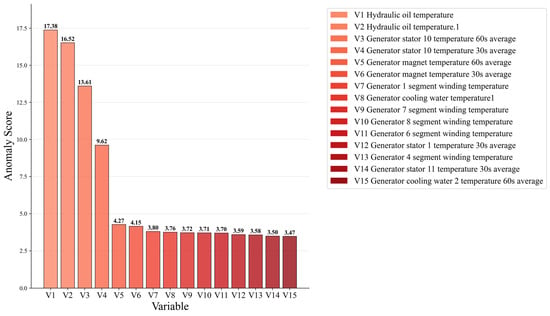
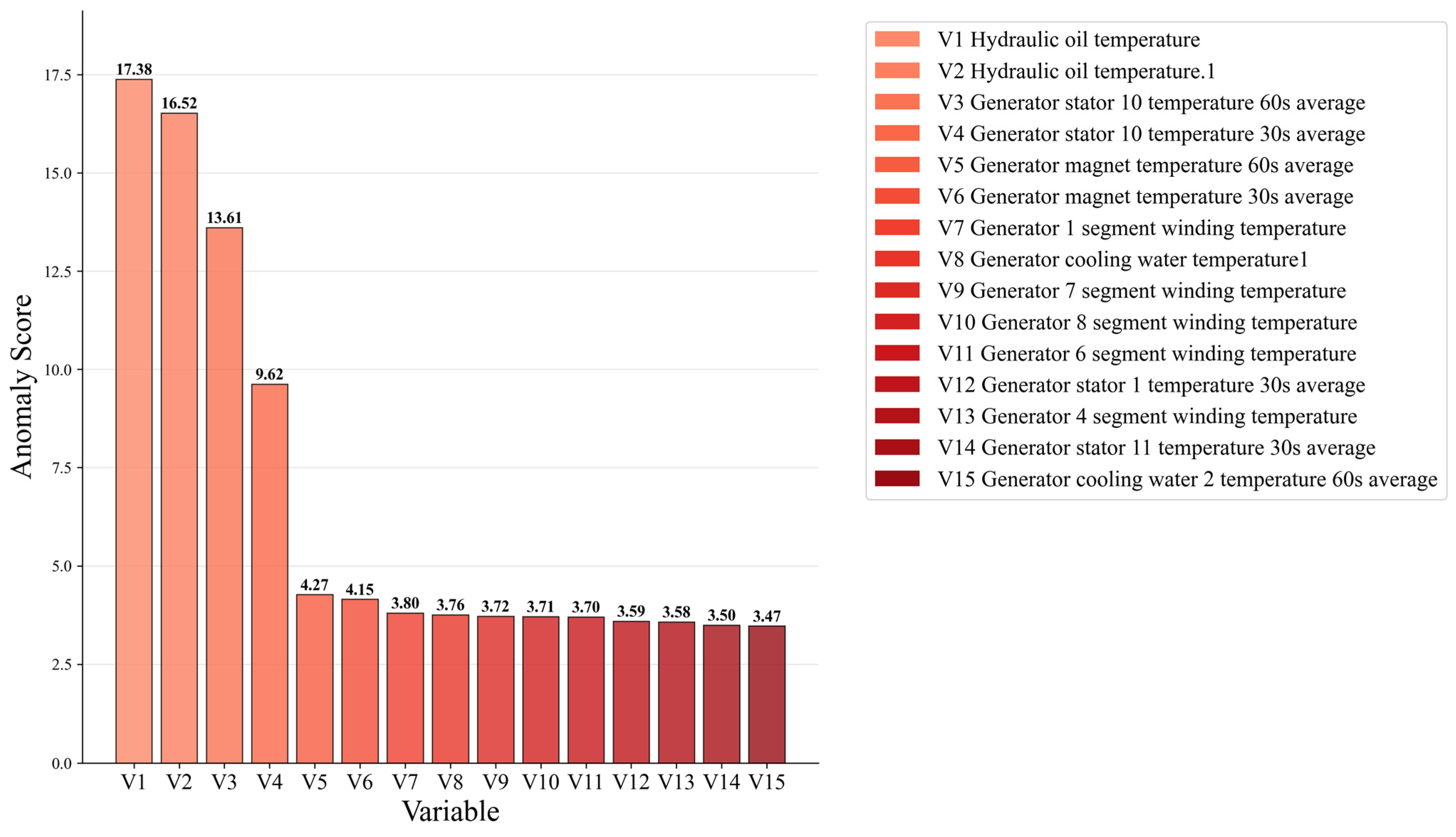
In order to locate the faulty parts of the wind turbine generator, we process the logarithmic density of each variable and sort the abnormal scores after variable level normalization, due to the space problem, the results of the first 15 results will be intercepted with the abnormal scores sorted from high to low, and the display results are shown in Figure 8, and it can be found that the abnormal scores with high scores are respectively the hydraulic oil temperature, generator stator temperature, generator magnet temperature, generator winding temperature, etc., are identified as abnormal nodes, which coincide with the information in the SCADA warning, indicating that the method proposed in this paper can effectively perform fault localization.

Figure 8. Ranking the anomaly scores of variables according to the proposed variational approach.

4.2. Ablation Study

To rigorously evaluate the contribution of each core component in the proposed CSDG-VNF framework, we conduct a series of ablation experiments on the same dataset under identical training and evaluation protocols. Three variants are compared:

Removes the causal masking in the temporal attention module, allowing future information to influence past representations. The abnormal score curve is shown in Figure 9.

Figure 9. Calculation of anomaly score curves for the causal masking removal module.

Replaces the dynamic graph convolution with a simple concatenation or MLP-based fusion of spatial and temporal features, disabling explicit inter-variable relational modeling. The abnormal score curve is shown in Figure 10.

Figure 10. Calculation of anomaly score curves excluding dynamic image convolution modules.

Replaces the variable-level normalized flow with a standard Gaussian Mixture Model (GMM) for joint density estimation, losing per-variable anomaly sensitivity. The abnormal score curve is shown in Figure 11.

Figure 11. Calculation of anomaly score curves excluding variable-level normalization flow modules.

Performance evaluation metrics include AUC values for two types of fault events and early detection lead time (unit: minutes). The complete CSDG-VNF model achieved the highest AUC value (0.991) and the longest average lead time (57.5 min). Removing any component resulted in significant performance degradation:

Eliminating causal masking (DG-VNF) reduced AUC by 1.3%. Disabling dynamic graph convolutions (CS-VNF) decreased AUC by 3.8%, confirming that explicitly modeling variable dependencies is crucial for capturing global anomalies. Replacing variable-level normalized flows (CSDG-GMM) caused a 9.1% AUC drop and failed to accurately localize faults, resulting in multiple misclassifications.

These results quantitatively validate that all three modules are indispensable. Their synergistic integration achieves both high-precision anomaly detection and accurate fault localization.

4.3. Computational Complexity

The computational costs of the proposed method and the compared methods are further evaluated in this section. All experiments are conducted on the NVIDIA GeForce RTX 4060 GPU. Unless otherwise specified, the model was trained for 300 epochs with batch size B = 8 using the Adam optimizer with an initial learning rate of 0.01. The average training time and inference time of different methods are listed in Table 3.

Table 3. Computation efficiency of different methods.

Method	Training Time (s/epoch)	Inference Time (s)
CSDG-VNF	27.42	0.84
DG-VNF	25.49	0.87
LSTM-CNN	6.23	0.13

We observe that compared to the baseline results mentioned earlier, both DG-VNF and the proposed CSDG-VNF require longer training times than LSTM-CNN. However, in terms of AUG scores, the proposed method outperforms both DG-VNF and LSTM-CNN. Although the proposed DG-VNF requires longer training time than LSTM-CNN due to the introduction of spatio-temporal self-attention and variable-level normalization flow, this duration remains acceptable in offline training scenarios.

5. Conclusions

This paper proposes a graph learning model and a variable-level normalized flow anomaly identification and fault localization model for a spatio-temporal attention mechanism under causality. Experimental validation is carried out through SCADA data cases of relevant wind turbine generators in China. In conclusion, the CSDG-VNF framework effectively addresses the challenges of spatio-temporal dependency modeling and causal consistency in wind turbine fault detection. Quantitative evaluation shows it achieves an AUC of 0.991 on real-world SCADA data and provides early warnings over 50 min before actual failures, significantly outperforming existing approaches such as DG-VNF and LSTM-CNN. These results validate its practical value for improving wind turbine reliability and reducing maintenance costs. Moreover, the method can also accomplish the localization of wind turbine faults. The method in the paper is able to extract and fuse spatio-temporal features, but it does not achieve abnormal diagnosis and identification with few samples and few labels, and the classification of fault types is not accurate, and it lacks the ability to learn and diagnose new types of faults, future research can start to improve the intelligence level of the model to realize the diagnosis and identification of faults with few samples and few labels, and it can start to improve the self-learning ability of the model to learn and diagnose new fault types. self-learning and diagnosis of new fault types.

References

- Zhang, H.; Guo, X.; Zhang, P. Improved PSO-SVM-Based Fault Diagnosis Algorithm for Wind Power Converter. In Proceedings of the 4th International Conference on Smart Power and Internet Energy Systems (SPIES); IEEE: Piscataway, NJ, USA, 2022. [Google Scholar]
- Yu, D.; Chen, Z.; Xiahou, K.; Li, M.; Ji, T.; Wu, Q. A radically data-driven method for fault detection and diagnosis in wind turbines. Int. J. Electr. Power Energy Syst. 2018, 99, 577–584. [Google Scholar] [CrossRef] [Scilit]
- Liu, D.; Cui, L.; Chen, J. A novel generalized Vold-Kalman filtering for wind turbine fault diagnosis. Ocean Eng. 2024, 308, 118317. [Google Scholar] [CrossRef] [Scilit]
- Dibaj, A.; Gao, Z.; Nejad, A.R. Fault detection of offshore wind turbine drivetrains in different environmental conditions through optimal selection of vibration measurements. Renew. Energy 2023, 203, 161–176. [Google Scholar] [CrossRef] [Scilit]
- Sun, S.; Wang, T.; Chu, F. In-situ condition monitoring of wind turbine blades: A critical and systematic review of techniques, challenges, and futures. Renew. Sustain. Energy Rev. 2022, 160, 112326. [Google Scholar] [CrossRef] [Scilit]
- Reder, M.; Yürüşen, N.Y.; Melero, J.J. Data-driven learning framework for associating weather conditions and wind turbine failures. Reliab. Eng. Syst. Saf. 2018, 169, 554–569. [Google Scholar] [CrossRef] [Scilit]
- Khan, P.W.; Byun, Y.C. Fault prognosis of wind turbines using multimodal machine learning. Energy Rep. 2024, 12, 4938–4952. [Google Scholar] [CrossRef] [Scilit]
- Yang, Z.; Baraldi, P.; Zio, E. A method for fault detection in multi-component systems based on sparse autoencoder-based deep neural networks. Reliab. Eng. Syst. Saf. 2022, 220, 108278. [Google Scholar] [CrossRef] [Scilit]
- Zhang, W.; Peng, G.; Li, C.; Chen, Y.; Zhang, Z. A New Deep Learning Model for Fault Diagnosis with Good Anti-Noise and Domain Adaptation Ability on Raw Vibration Signals. Sensors 2017, 17, 425. [Google Scholar] [CrossRef] [Scilit]
- Wang, T.; Yin, L. A hybrid 3DSE-CNN-2DLSTM model for compound fault detection of wind turbines. Expert Syst. Appl. 2024, 242, 122776. [Google Scholar] [CrossRef] [Scilit]
- Minh, T.Q.; Van, T.N.; Nguyen, H.X.; Nguyễn, Q. Enhancing the Structural Health Monitoring (SHM) through data reconstruction: Integrating 1D convolutional neural networks (1DCNN) with bidirectional long short-term memory networks (Bi-LSTM). Eng. Struct. 2025, 340, 120767. [Google Scholar] [CrossRef] [Scilit]
- Feng, C.; Liu, C.; Jiang, D. Root cause localization for wind turbines using physics guided multivariate graphical modeling and fault propagation analysis. Knowl.-Based Syst. 2024, 295, 111838. [Google Scholar] [CrossRef] [Scilit]
- Zhu, Y.; Xie, B.; Wang, A.; Qian, Z. Wind turbine fault detection and identification via self-attention-based dynamic graph representation learning and variable-level normalizing flow. Reliab. Eng. Syst. Saf. 2025, 253, 110554. [Google Scholar] [CrossRef] [Scilit]
- Streser, E.; Alipek, S.; Rao, M.; Simon, J.; Moll, J.; Kraemer, P.; Krozer, V. Radar-Based Damage Detection in a Wind Turbine Blade Using Convolutional Neural Networks: A Proof-of-Concept Under Fatigue Loading. Sensors 2025, 25, 3337. [Google Scholar] [CrossRef] [Scilit]
- Rizk, P.; Rizk, F.; Karganroudi, S.S.; Ilinca, A.; Younes, R.; Khoder, J. Advanced wind turbine blade inspection with hyperspectral imaging and 3D convolutional neural networks for damage detection. Energy AI 2024, 16, 100366. [Google Scholar] [CrossRef] [Scilit]
- Wang, A.; Pei, Y.; Zhu, Y.; Qian, Z. Wind turbine fault detection and identification through self-attention-based mechanism embedded with a multivariable query pattern. Renew. Energy 2023, 211, 918–937. [Google Scholar] [CrossRef] [Scilit]
- Schlechtingen, M.; Ferreira Santos, I. Comparative analysis of neural network and regression based condition monitoring approaches for wind turbine fault detection. Mech. Syst. Signal Process. 2011, 25, 1849–1875. [Google Scholar] [CrossRef] [Scilit]
- Wang, T.; Chu, F.; Han, Q. Fault diagnosis for wind turbine planetary ring gear via a meshing resonance based filtering algorithm. ISA Trans. 2017, 67, 173–182. [Google Scholar] [CrossRef] [Scilit] [PubMed]
- Palanimuthu, K.; Mayilsamy, G.; Lee, S.R.; Jung, S.Y.; Joo, Y.H. Fault Ride-Through for PMVG-Based Wind Turbine System Using Coordinated Active and Reactive Power Control Strategy. IEEE Trans. Ind. Electron. 2023, 70, 5797–5807. [Google Scholar] [CrossRef] [Scilit]
- Sheng, L.; Li, C.; Gao, M.; Xi, X.; Zhou, D. A review of SCADA-based condition monitoring for wind turbines via artificial neural networks. Neurocomputing 2025, 633, 129830. [Google Scholar] [CrossRef] [Scilit]
- Qi, L.; Zhang, Q.; Xie, Y.; Zhang, J.; Ke, J. Research on Wind Turbine Fault Detection Based on CNN-LSTM. Energies 2024, 17, 4497. [Google Scholar] [CrossRef] [Scilit]
- Yang, T.; Ying, Y. AUC Maximization in the Era of Big Data and AI: A Survey. ACM Comput. Surv. 2022, 55, 172. [Google Scholar] [CrossRef] [Scilit]
Disclaimer/Publisher’s Note: The statements, opinions and data contained in all publications are solely those of the individual author(s) and contributor(s) and not of MDPI and/or the editor(s). MDPI and/or the editor(s) disclaim responsibility for any injury to people or property resulting from any ideas, methods, instructions or products referred to in the content. |
© 2026 by the authors. Licensee MDPI, Basel, Switzerland. This article is an open access article distributed under the terms and conditions of the Creative Commons Attribution (CC BY) license.