


Abstract
In this work, we present the procedure to obtain exact spherical shape functions for finite element modeling applications, without resorting to any kind of approximation, for generic prismatic spherical elements and for the case of spherical six-node tri-rectangular and eight-node quadrangular spherical prisms. The proposed spherical shape functions, given in explicit analytical form, are expressed in geographic coordinates, namely colatitude, longitude and distance from the center of the sphere. We demonstrate that our analytical shape functions satisfy all the properties required by this class of functions, deriving at the same time the analytical expression of the Jacobian, which allows us changes in coordinate systems. Within the perspective of volume integration on Earth, entering a variety of geophysical and geodetic problems, as for mass change contribution to gravity, we consider our analytical expression of the shape functions and Jacobian for the six-node tri-rectangular and eight-node quadrangular right spherical prisms as reference volumes to evaluate the volume of generic spherical triangular and quadrangular prisms over the sphere; volume integration is carried out via Gauss–Legendre quadrature points. We show that for spherical quadrangular prisms, the percentage volume difference between the exact and the numerically evaluated volumes is independent from both the geographical position and the depth and ranges from 10−3 to lower than 10−4 for angular dimensions ranging from 1° × 1° to 0.25° × 0.25°. A satisfactory accuracy is attained for eight Gauss–Legendre quadrature points. We also solve the Poisson equation and compare the numerical solution with the analytical solution, obtained in the case of steady-state heat conduction with internal heat production. We show that, even with a relatively coarse grid, our elements are capable of providing a satisfactory fit between numerical and analytical solutions, with a maximum difference in the order of 0.2% of the exact value.
1. Introduction
A number of 3D finite element models have been developed in the last decades in the attempt to simulate large-scale geodynamic processes. Most of them, however, account for a flat Earth, e.g., refs. [1,2,3,4,5,6,7,8,9]. Sphericity is, on the other hand, one main property of the planet that needs to be implemented when dealing with global geophysical problems. Pure radial variations of the physical properties of the Earth, in terms of distance from the center of the planet, can be dealt with via analytical methods, where the independent functions constituting the basis over which each field is expanded can be, for example, the spherical harmonics. Only a few finite element methods are available, e.g., refs. [10,11,12,13], which account for the sphericity of the Earth at the global scale, but at the local scale of each element, sphericity is only approximated.
To handle physical properties that vary along latitude and longitude, beyond the radial direction, appropriate spherical shape functions that interpolate the vectoral fields onto a spherical surface are required. Within this study, we propose the analytical expressions of new spherical shape functions for generic spherical prismatic elements and for the specific case of reference spherical six-node tri-rectangular and eight-node quadrangular prisms. The latter can be used as reference elements within a finite element algorithm: from this perspective, we also derive the explicit analytical expression of the Jacobian matrix as a function of the radius, latitude and longitude.
The proposed procedure for determining the expressions of the shape functions in a spherical coordinate system follows the well-known procedure developed in a Cartesian space and found in classical texts on finite element methods, e.g., refs. [14,15], adapting it to a spherical coordinate system and considering the fact that quantities are interpolated on a spherical surface instead of a flat one.
2. Mathematical Formulation
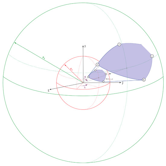
Consider the generic spherical prismatic element in Figure 1, bounded by two polygonal spherical surfaces with n vertexes and located over two spheres of radius r1 and r2, and (n − 1) flat surfaces along the radial direction, and denote with the spherical shape functions, with colatitude, longitude and radius of the sphere varying between r1 and r2.
Figure 1.
Generic spherical prismatic element. The inner and the outer spheres of radius r1 and r2, where the base and the top of the spherical prismatic element are located, are indicated in red and green colors, respectively.
Since interpolation of a vector quantity on a spherical surface necessitates accounting for the different orientations of the unit vectors normal and tangent to the surface, here, we assume that the shape functions can be expressed as the product of three functions such that
where and are scalar functions expressing, respectively, the variation of N with the radial distance from the center of the sphere and with the colatitude and longitude when moving from one point to another inside the element. is a matrix function accounting for the variation of with the variation of the orientation of the unit vector normal to surface when moving from one point to another on the sphere. In the following sections, we will describe the procedure we propose to define functions , and .
2.1. Functions R(r)
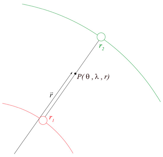
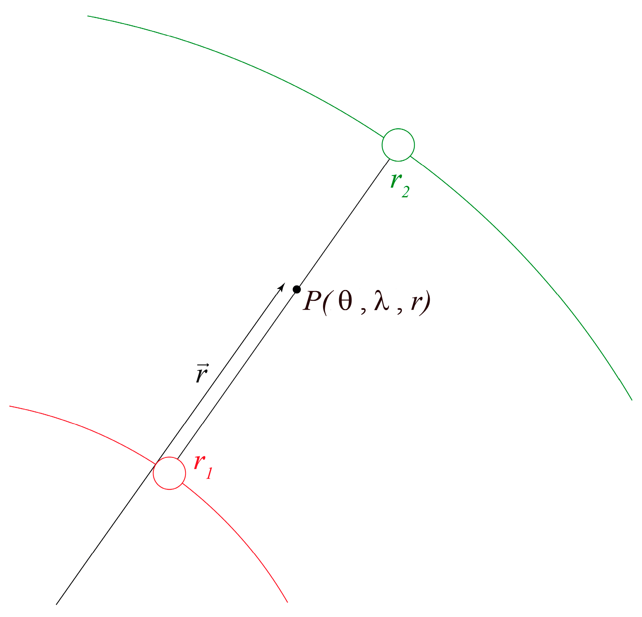
Functions account for the radial variation of . We here propose to express them in terms of linear variation along the r direction (Figure 2), such that
with
Figure 2.
1D element along the radial direction. and are the radii of the inner (red color) and outer (green color) spheres.
2.2. Functions F(θ,λ)
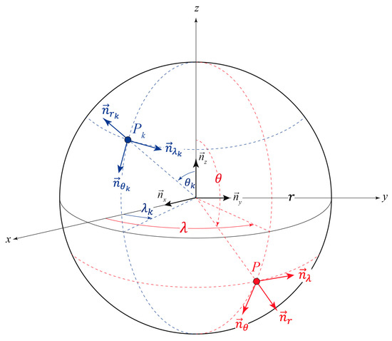
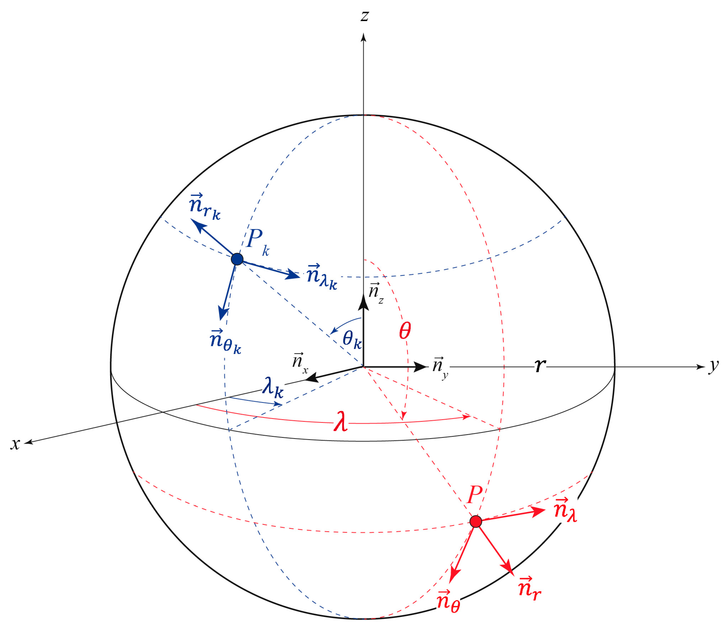
When a vector quantity is interpolated from one point to another over a sphere, it is necessary to account for the different orientations of the unit vectors normal and tangent to the surface at the two points, as shown in Figure 3.
Figure 3.
Scheme illustrating the variation of the orientation of unit vector normal to the sphere surface moving from point P to point Pk.
Let us consider the rotation matrix
that maps the Earth-Centered Rotational Reference Frame into the Centered P-Rotational Reference Frame , such that
Similarly, let us consider its inverse matrix
that maps the Centered P-Rotational Reference Frame into the Earth-Centered Rotational Reference Frame, such that
Moving from point to point of coordinates over a sphere requires a double rotation of the displacement vector at .
Let denote the displacement at point . Its expression in the -centered reference frame can therefore be expressed as
The function that makes it possible to walk over the surface of the sphere from one generic point to any other generic point , in terms of the components of any vectoral quantity, typically displacements and velocities in geophysics, is thus
or, after a few mathematical steps,
2.3. Functions A(θ,λ)
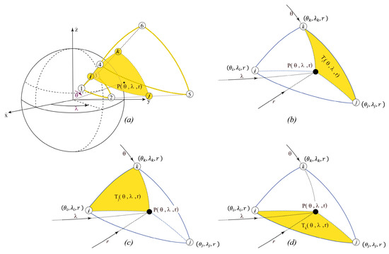
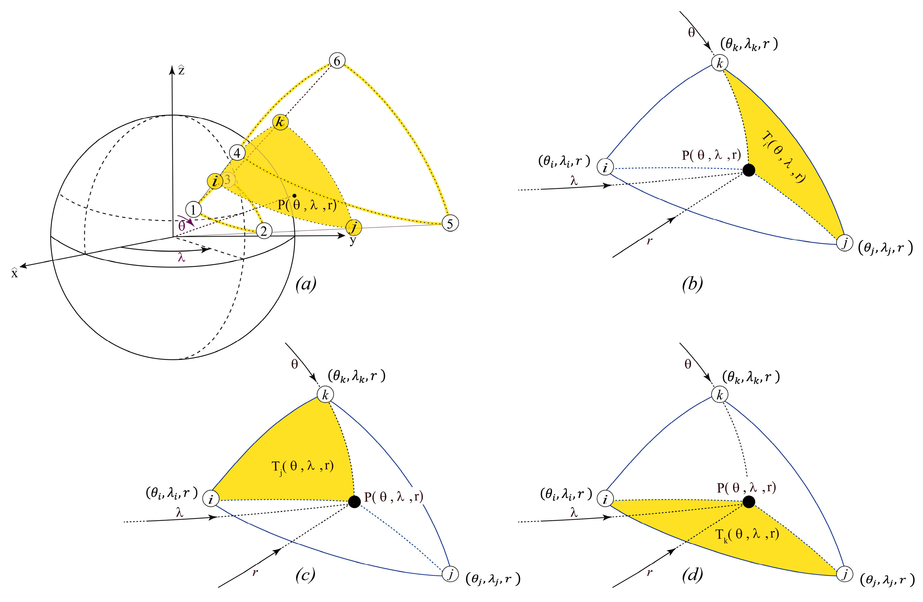
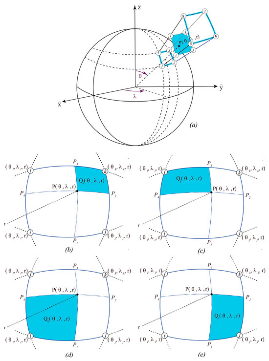
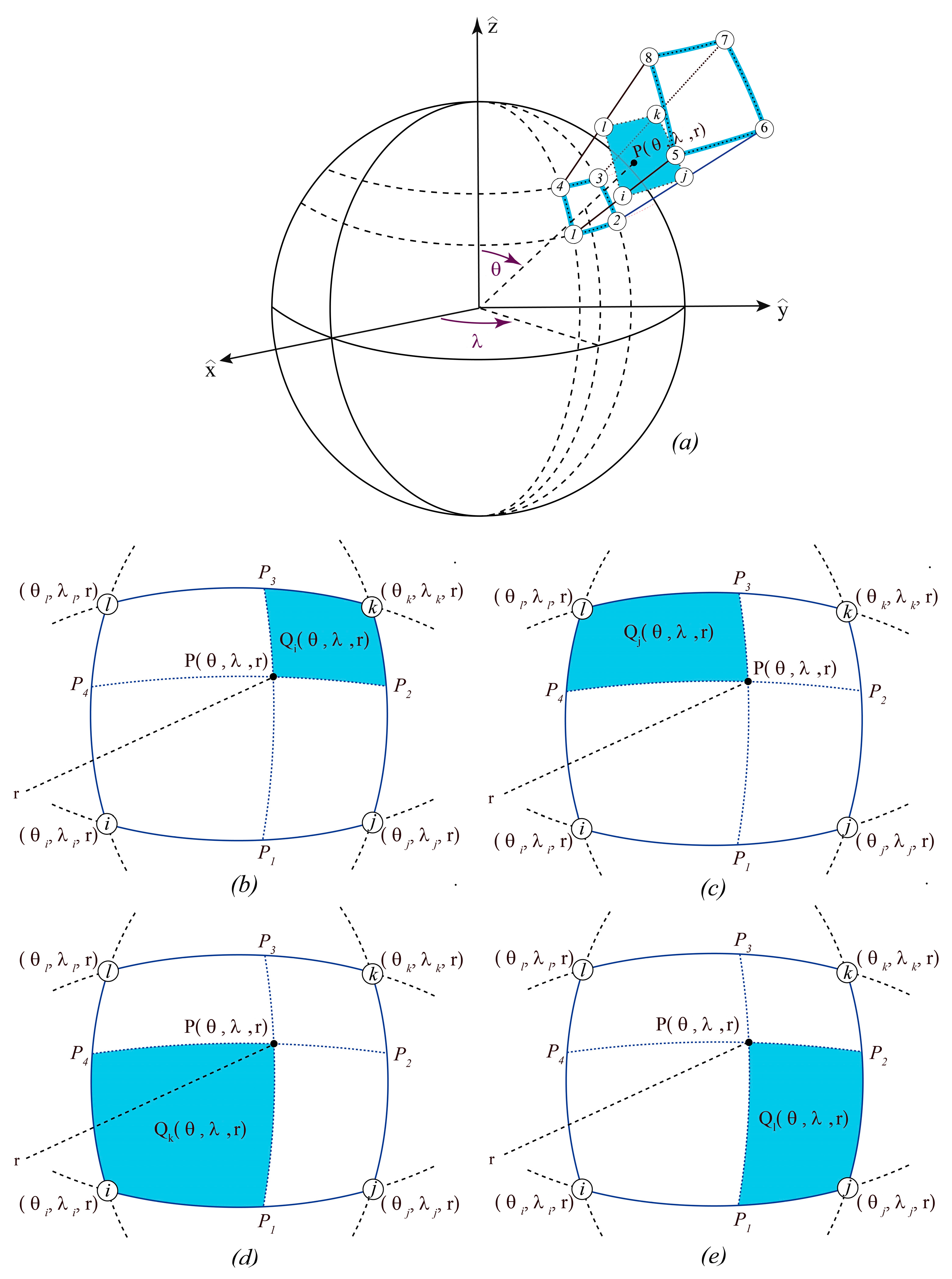
We here derive the expressions of functions for spherical six-node triangular and eight-node quadrangular right prisms (panels a in Figure 4 and Figure 5, respectively).
Figure 4.
(a) Scheme of a generic six-node triangular prism. (b) Spherical triangle (gold color) whose area is defined in Equations (17) and (18). (c) Spherical triangle (gold color) whose area is defined in Equations (19) and (20). (d) Spherical triangle (gold color) whose area is defined in Equations (21) and (22).
Figure 5.
(a) Scheme of a generic eight-node rectangular right prism. (b) Spherical right rectangle (blue color) whose area is defined in Equation (25). (c) Spherical right rectangle (blue color) whose area is defined in Equation (26). (d) Spherical right rectangle (blue color) whose area is defined in Equation (27). (e) Spherical right rectangle (blue color) whose area is defined in Equation (28).
2.3.1. Spherical Six-Node Triangular Prism
Let us consider the spherical six-node triangular prism shown in panel a in Figure 4 and the spherical triangle with vertices (i, j, k). Using an approach that is similar to that used in the planar configuration (e.g., [14]), we express as
where
denotes the area of the spherical triangle , panel a in Figure 4, with
2.3.2. Spherical Eight-Node Quadrangular Right Prism
Consider the eight-node quadrangular prism shown in Figure 5, with sides parallel to the geographic parallels and meridians, and the spherical right rectangle with vertices (i, j, k, l). Functions can be expressed as
where
is the area of spherical right rectangle , panel a in Figure 5;
is the area of spherical right rectangle , panel b in Figure 5;
is the area of spherical right rectangle , panel c in Figure 5;
is the area of spherical right rectangle , panel d in Figure 5;
is the area of spherical right rectangle , panel e in Figure 5.
Considering that , the final expressions of functions become
2.4. Shape Functions
We here derive the expressions of the shape functions for a spherical six-node tri-rectangular prism (Section 2.4.1) and for a spherical eight-node quadrangular right prism (Section 2.4.2).
2.4.1. Spherical Six-Node Tri-Rectangular Prism
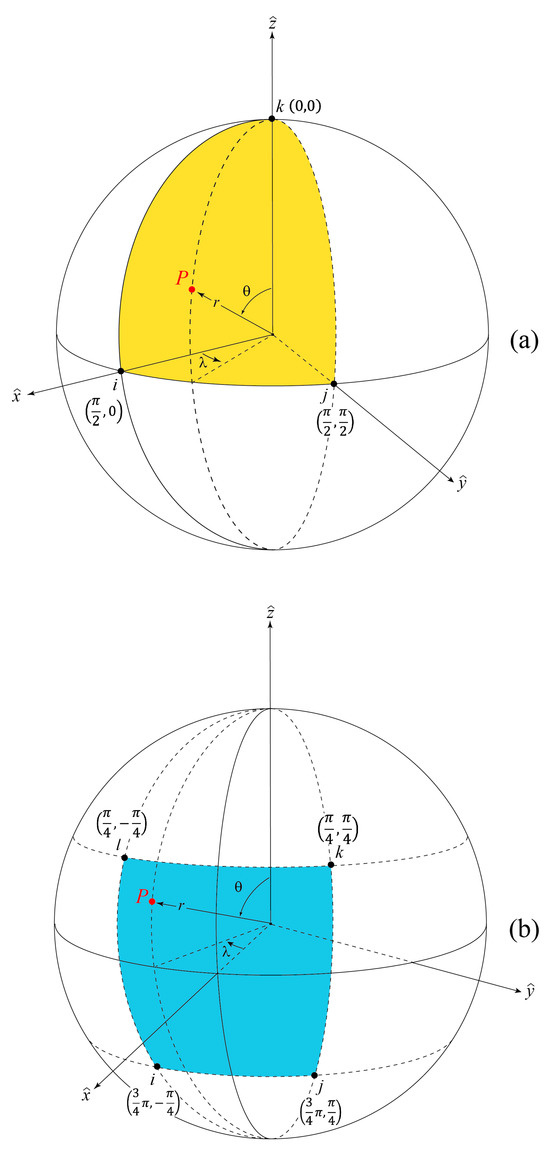
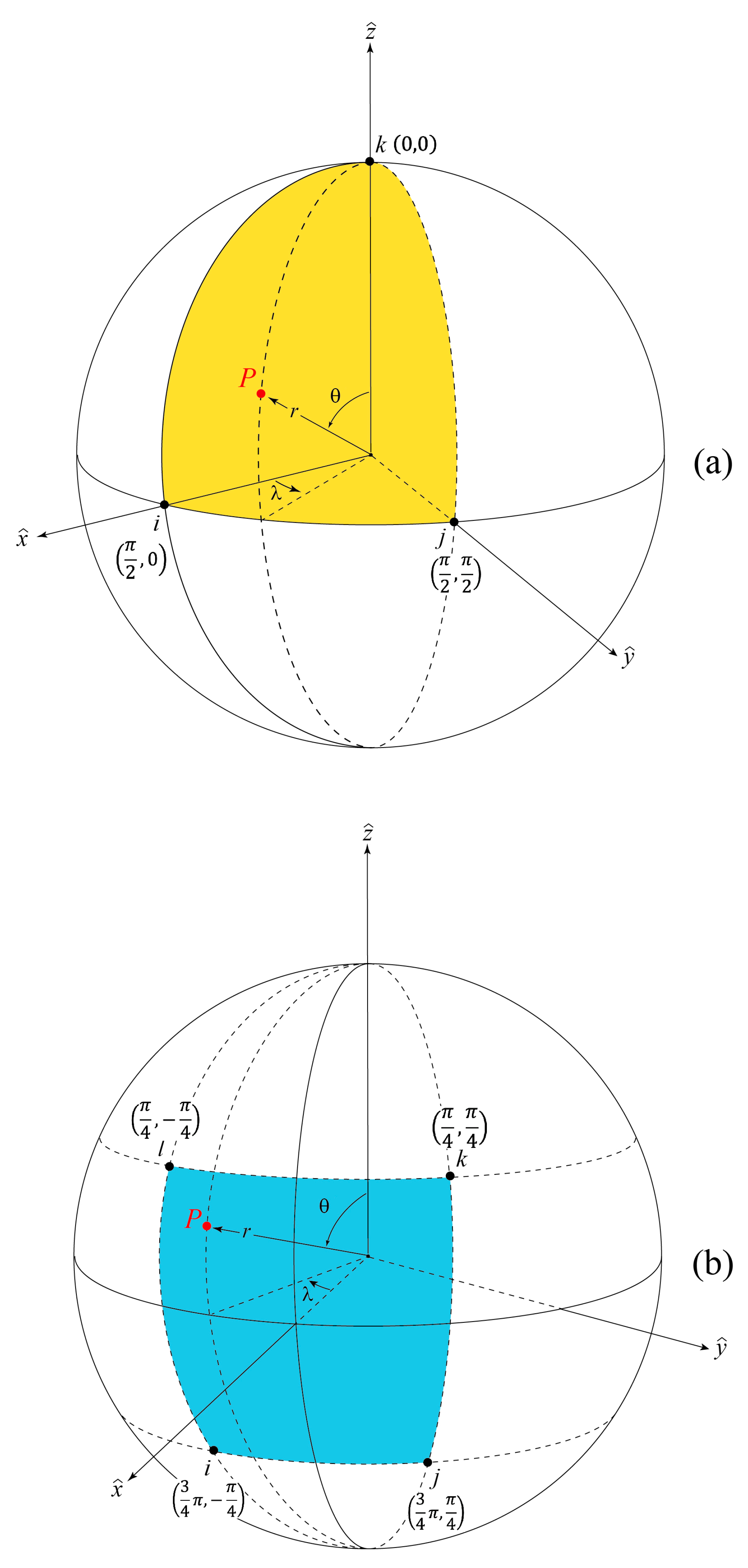
Assume that the triangular sides of the prism coincide with the spherical three-node tri-rectangular triangle in Figure 6 (panel a). The geographic coordinates of the nodes i, j and k become
Figure 6.
Scheme of a spherical six-node tri-rectangular prism (a) and a spherical eight-node rectangular right prism (b).
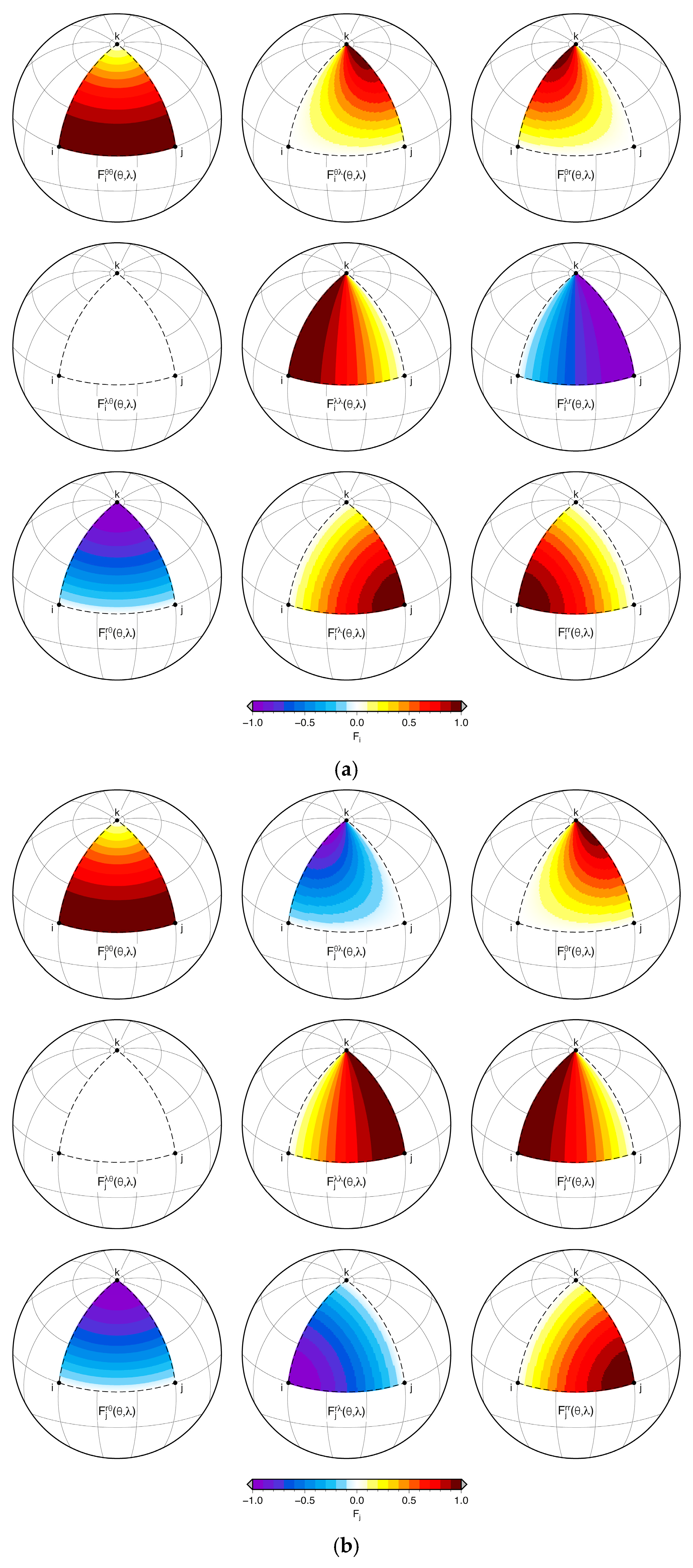
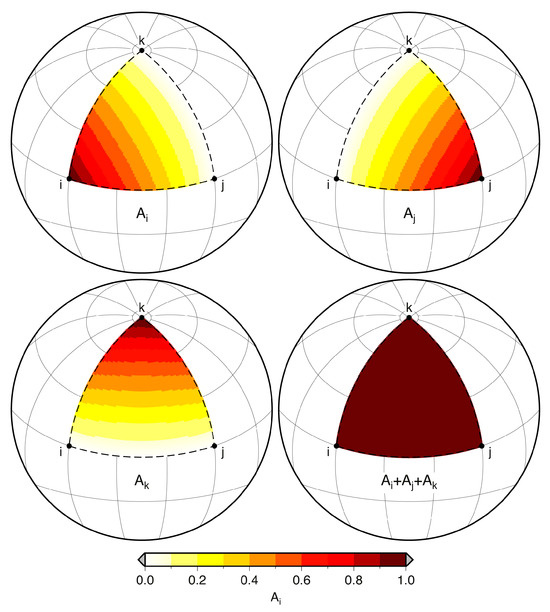
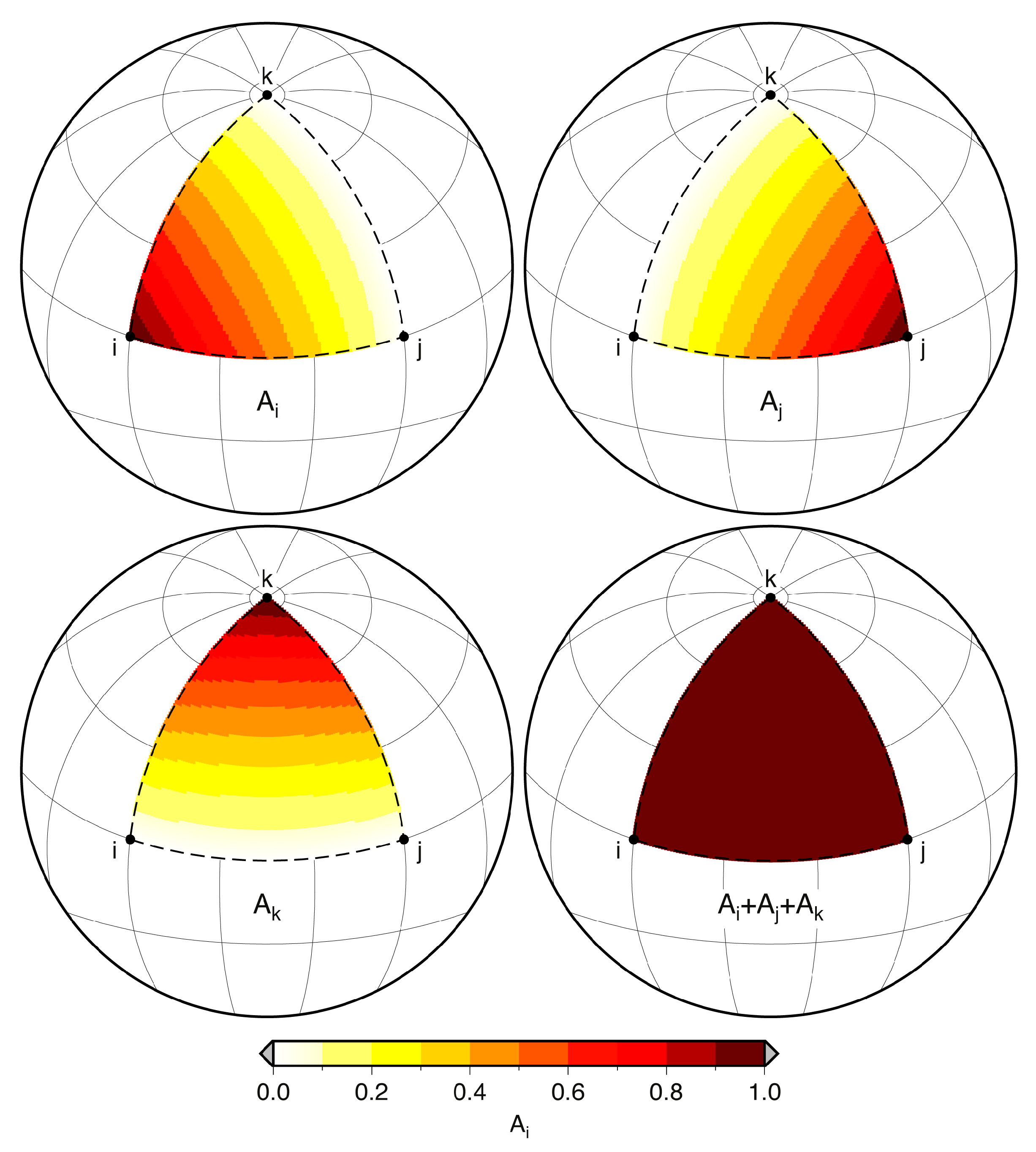
The expressions of functions (Equation (9)) reduce to
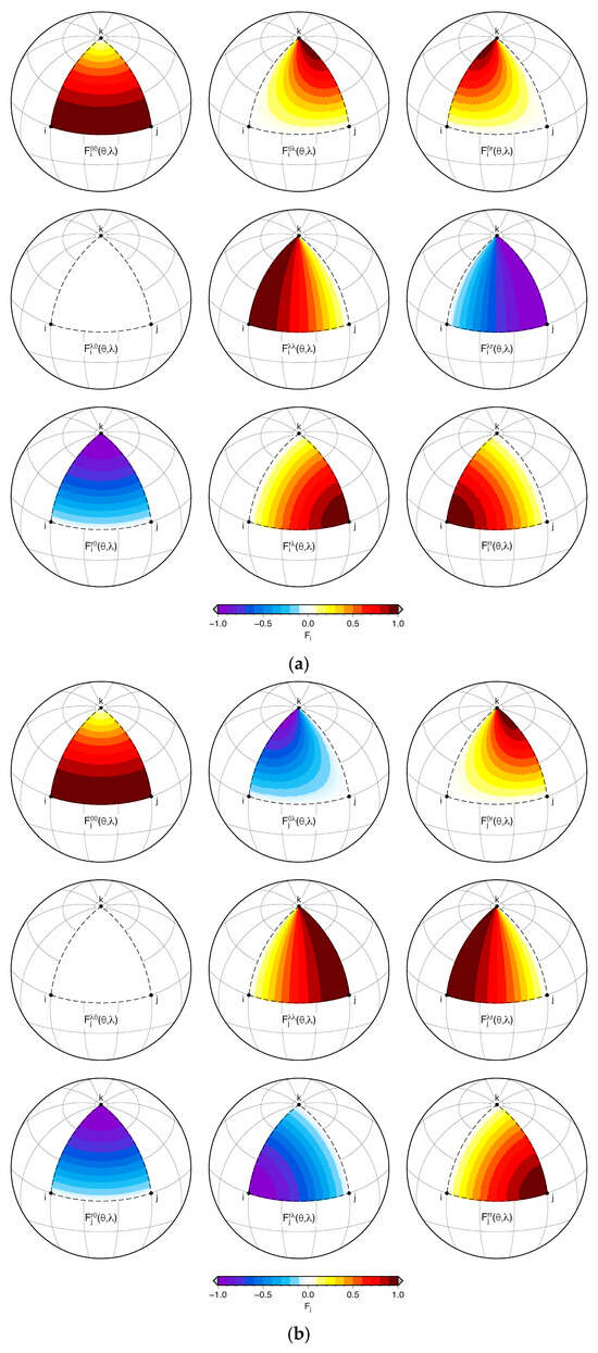
Figure 7a–c shows how functions vary smoothly with longitude and latitude.
Figure 7.
(a) Values of functions for a spherical six-node tri-rectangular prism. (b) Values of functions for a spherical six-node tri-rectangular prism. (c) Values of functions for a spherical six-node tri-rectangular prism.
It can be easily demonstrated that
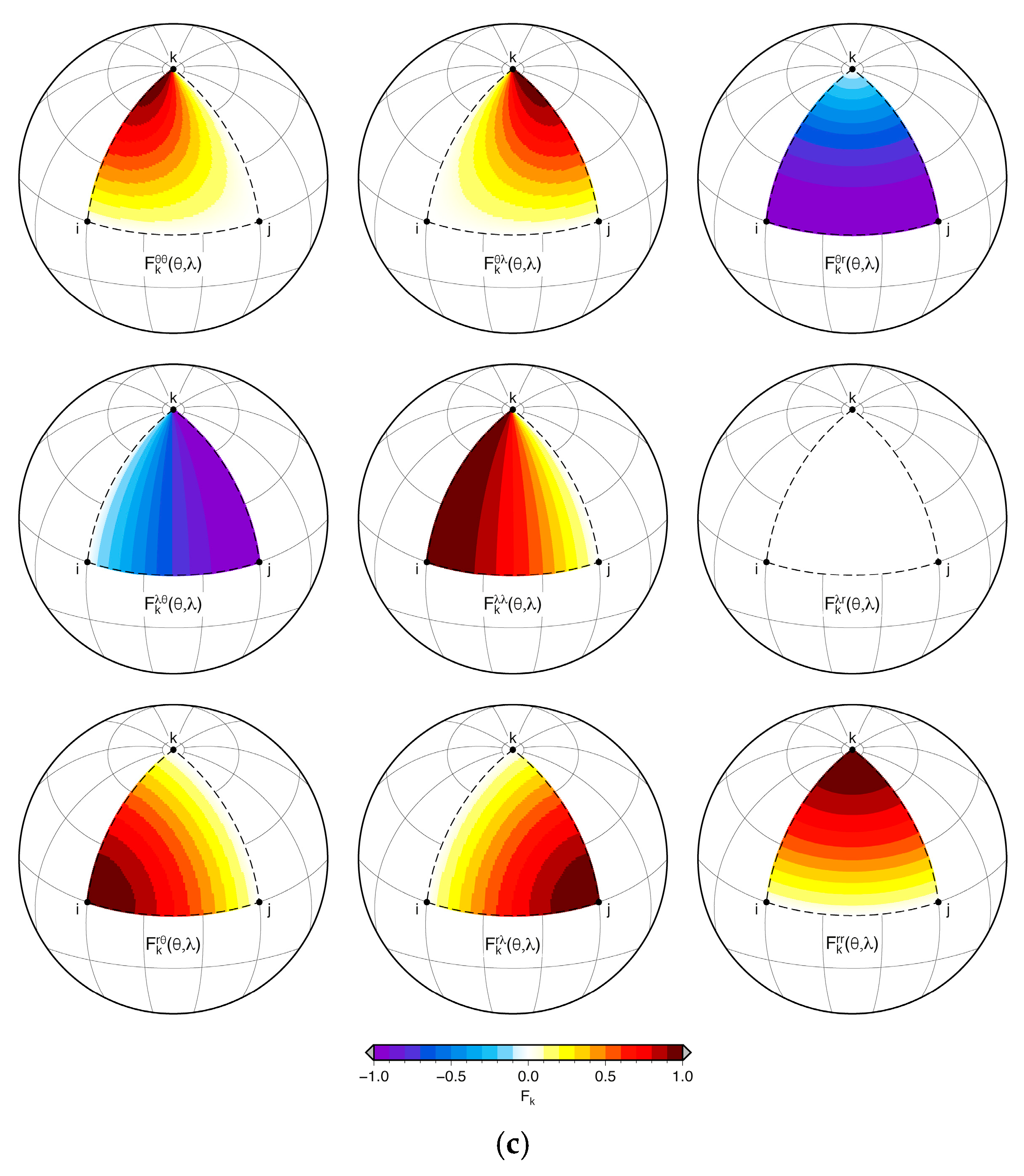
The expressions of function (Equation (11)) reduce to
The expression of the shape functions in (32) contains the term and in denominators that may lead the shape functions and their derivatives to have singularities. To make shape functions and derivatives remain finite at singular points, some checkpoints should be introduced into the algorithm to estimate the shape functions and their derivatives at each point of the elements. However, operatively, in finite element applications, the shape functions and their derivatives are calculated only at the quadrature points, which are always within the discretization basis element, and the conditions for the occurrence of singularities cannot occur.
It is trivial to demonstrate that
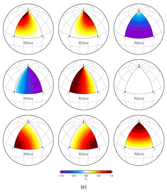
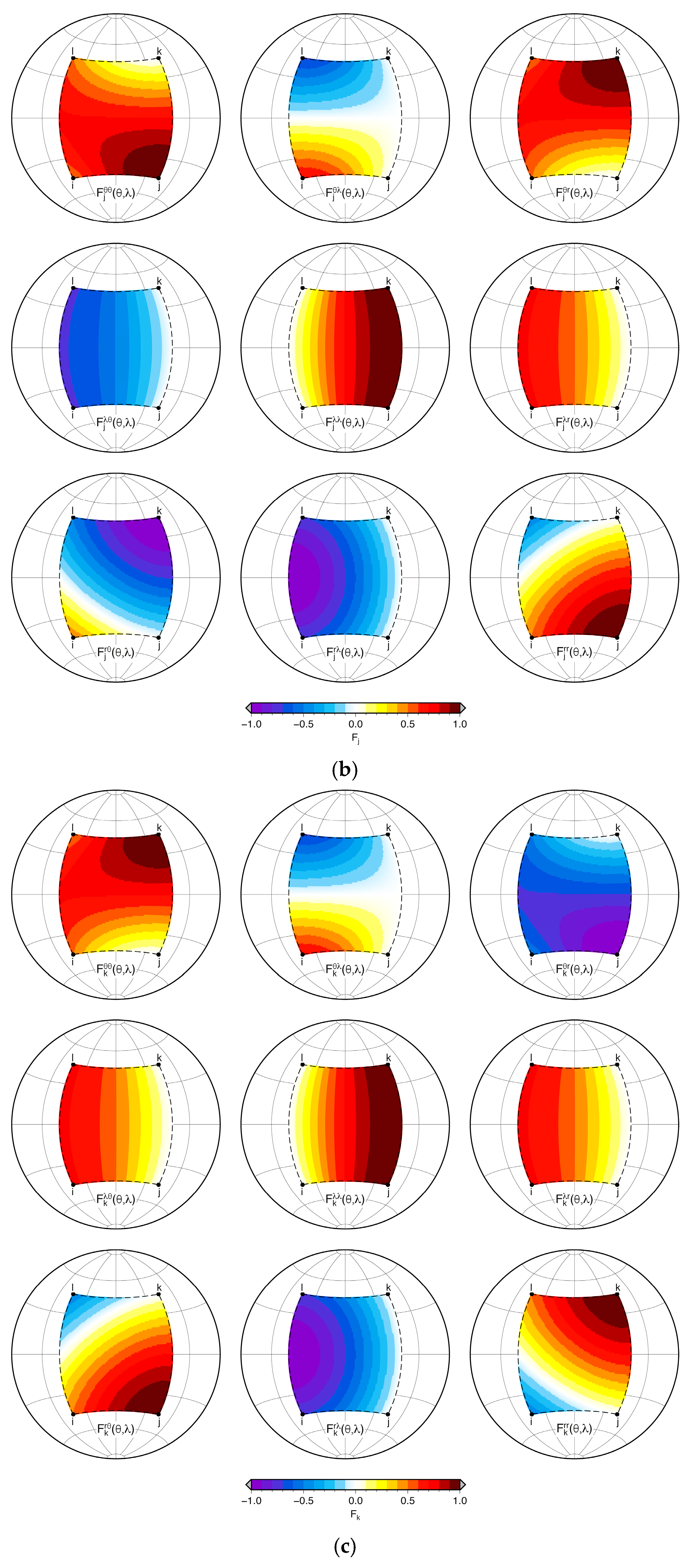
Figure 8 shows how functions vary with longitude and latitude within the assumed spherical tri-rectangular triangle.
Figure 8.
Values of functions for a spherical six-node tri-rectangular prism.
Based on Equation (1), the shape functions for a spherical six-node tri-rectangular prism can be expressed as
Based on Equations (3), (4), (31) and (33), it is trivial to demonstrate that
2.4.2. Spherical Eight-Node Quadrangular Right Prism—Tesseroid
Consider the spherical eight-node quadrangular right prism shown in Figure 6b. Assume that the sides of the prism coincide with the spherical rectangles of Figure 6b; the geographic coordinates of the nodes i, j, k and l become
Concerning functions (Equation (9)), they reduce to
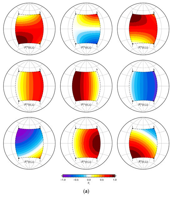
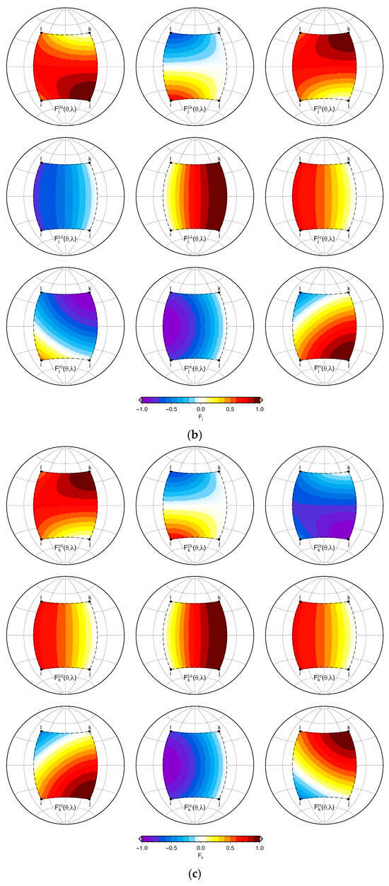
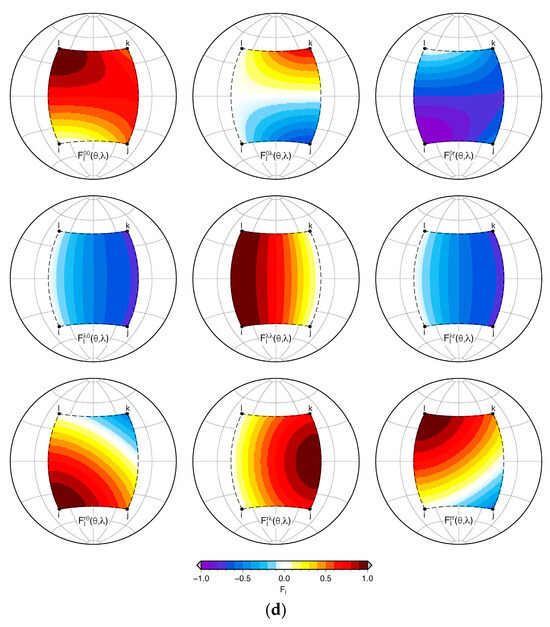
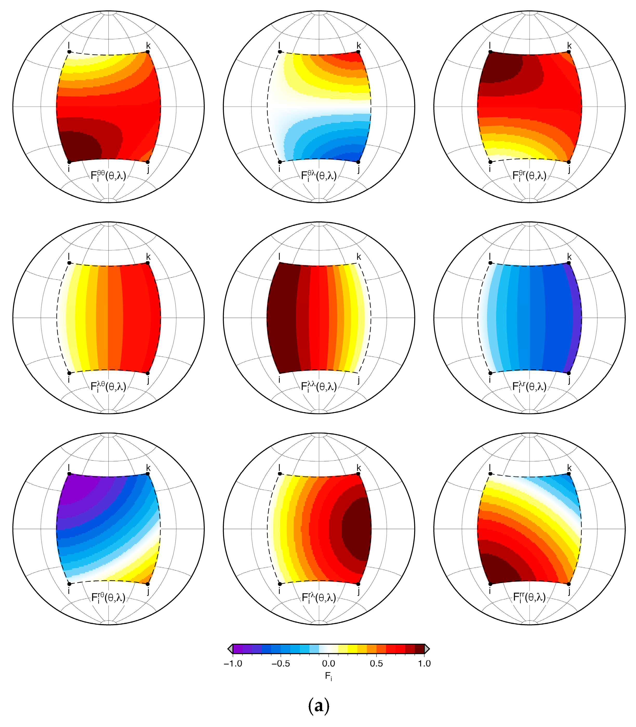
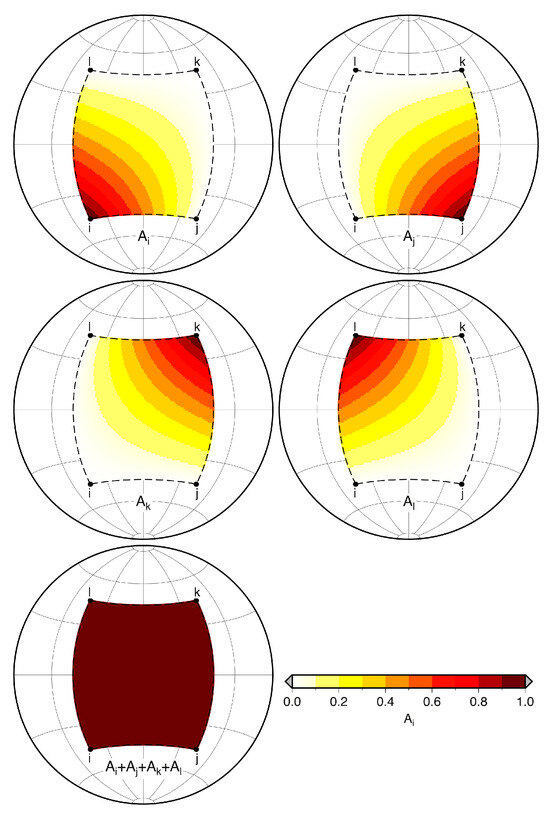
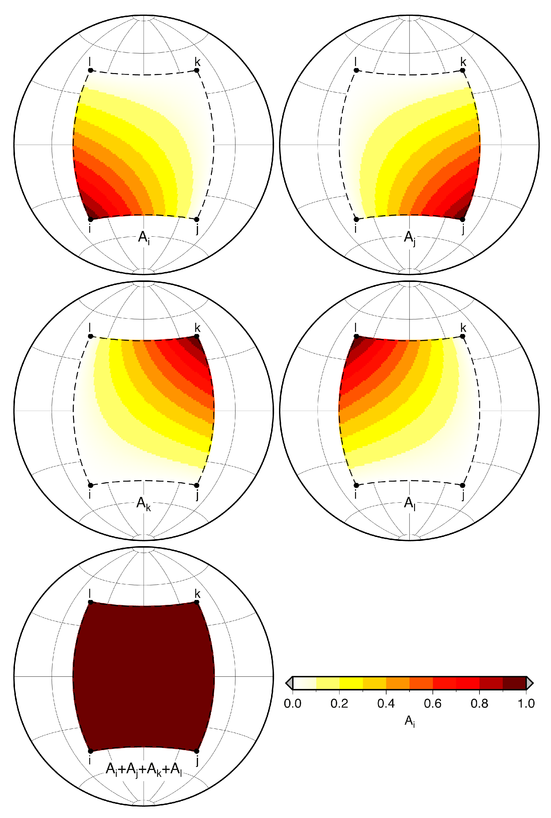
Figure 9a–d shows how functions vary smoothly with longitude and latitude within the assumed spherical rectangle.
Figure 9.
(a) Values of functions for a spherical eight-node quadrangular right prism. (b) Values of functions for a spherical eight-node quadrangular right prism. (c) Values of functions for a spherical eight-node quadrangular right prism. (d) Values of functions for a spherical eight-node quadrangular right prism.
It can be easily demonstrated that
The expressions of functions reduce to
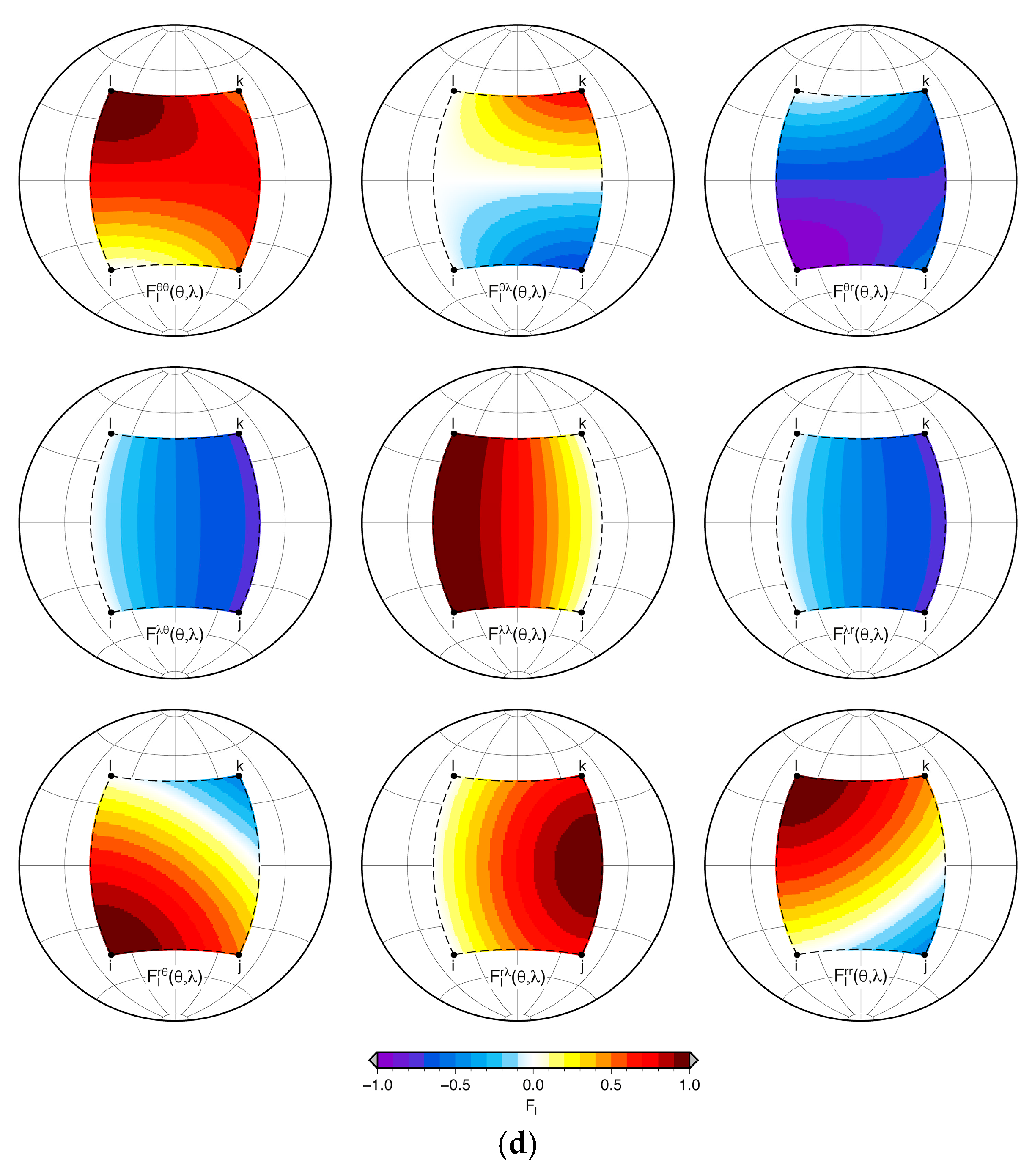
Figure 10 shows how functions vary with longitude and latitude within the assumed spherical rectangle.
Figure 10.
Values of functions for a spherical eight-node quadrangular right prism.
It is trivial to demonstrate that
Based on Equation (1), the shape functions for a spherical eight-node quadrangular right prism can be expressed as
Based on Equations (3), (4), (40) and (42), it is trivial to demonstrate that
3. Rigid Displacement on a Sphere
Assume a rigid displacement occurs on a sphere. If is the displacement at the generic point of coordinates , at any other point k, the displacement must be equal to
Thus, for a rigid displacement, the following expression holds
In conclusion, a rigid displacement implies that
For a spherical six-node tri-rectangular prism, it follows that
since
but
Thus, from Equation (33),
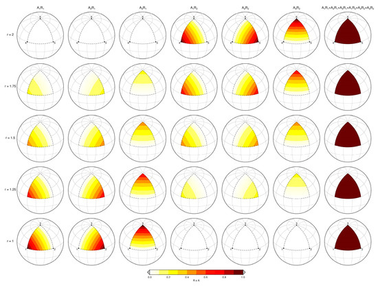
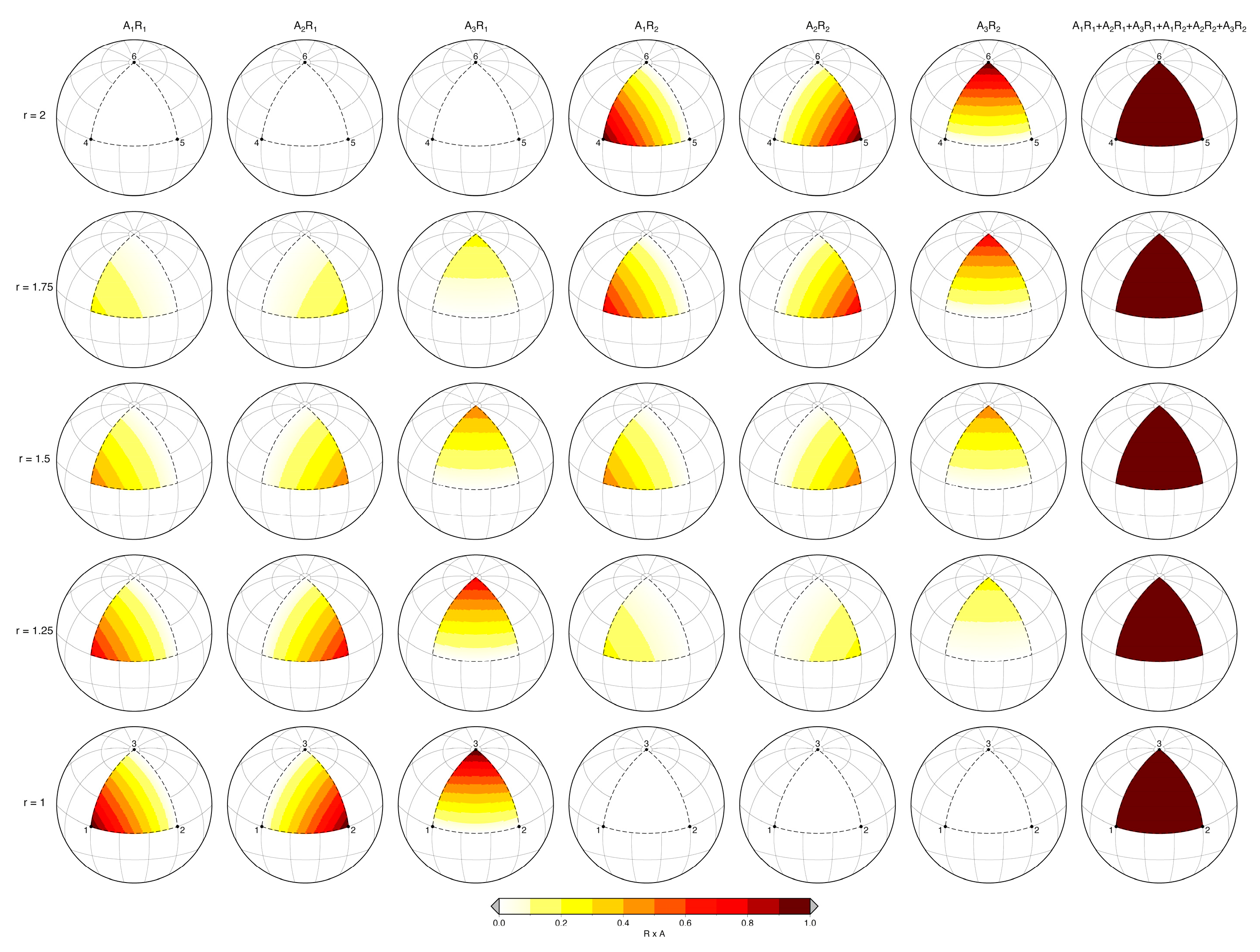
Figure 11 shows this result numerically for the spherical six-node tri-rectangular prism.
Figure 11.
Values of R(r)· for a spherical six-node tri-rectangular prism.
The same can be demonstrated for the spherical eight-node quadrangular prism:
since
on the basis of Equation (41).
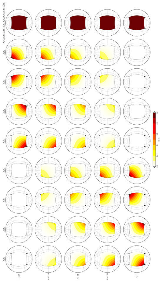
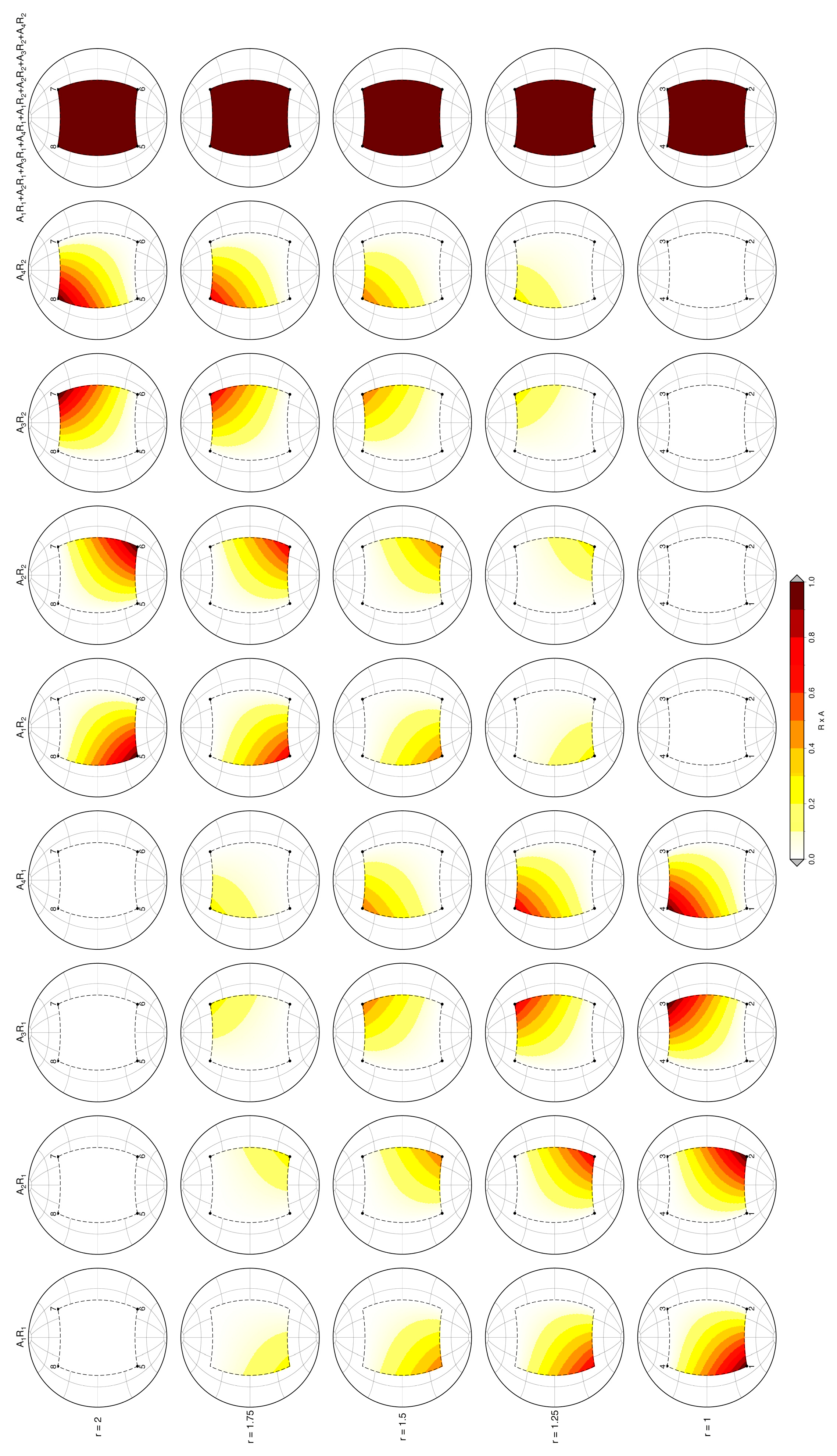
Figure 12 shows this result numerically for the eight-node quadrangular right prism.
Figure 12.
Values of R(r)· for a spherical eight-node quadrangular right prism.
We thus observe that at any point of any spherical surface at any depth within the volume, for both triangular and quadrangular, summation of the contribution from each component attains the value 1, as required by the partition of unity property of the shape functions [14].
4. Transformation from Global to Local Coordinates
The proposed shape functions above are defined into a local space. We here describe the procedure of transformation from the global space, where the problem is defined, to the local space of the shape functions.
Let us consider the spherical curvilinear coordinates in the local space
and the spherical curvilinear coordinates in the global space
Using the usual rules of partial differentiation, we can write
where J is the Jacobian matrix in spherical coordinates. The global spherical derivatives are thus defined as
The curvilinear coordinates of a generic point within each element can be expressed as
where nnode is the number of nodal connections of each element of the numerical grid.
The expression of the Jacobian, thus, becomes
or
4.1. Spherical Six-Node Tri-Rectangular Prism
Derivatives of :
Derivatives of :
4.2. Spherical Eight-Node Quadrangular Right Prism
Note that, as for the shape functions proposed for the spherical six-node tri-rectangular prisms and their derivatives, Jacobian expressions (61), (62) and (76) may have singularities if evaluated at the center of the sphere (r = 0) or at the poles (θ = 0 or 180). However, operationally, in finite element applications, the Jacobian is calculated only at the quadrature points, which are always within the discretization basis element, and the conditions for the occurrence of singularities cannot occur.
5. Infinitesimal Volume—Global to Local
Let us consider the point P on a sphere of global spherical coordinates . The position of P can be defined in terms of the curvilinear coordinates
evaluated along the directions of the meridian and of the parallel passing through P and of the line connecting P to the center of the sphere O, from O outwards. For any infinitesimal increment of the curvilinear coordinates the spherical infinitesimal volume can be expressed as
Assuming that the global curvilinear coordinates are functions of the local curvilinear coordinates of the reference element of the numerical grid defined in paragraphs 2, it follows that
The volume in the global space becomes
or, after a few mathematical steps,
6. Validation Tests
We have performed some validation tests in order to verify the performance of our analytical shape functions in evaluating the finite volumes of generic spherical prisms by which the real or a normalized Earth is discretized and the numerical solution of Poisson equation.
6.1. Volume
In these tests, we compare the value of the volume of a spherical prism calculated numerically using the Jacobian containing the derivatives of the shape functions proposed here and the volume of the same spherical prism calculated using the exact formula described below.
6.1.1. Spherical Triangular Prism
6.1.2. Spherical Quadrangular Prism–Tesseroid
While geometry is exact, numerical integration of transcendental functions remains approximate. We numerically perform the integral over the volume of the local reference element, taking advantage of the well-known Gauss–Legendre quadrature formula, where the n Gauss–Legendre points are the zeros of the Legendre polynomials, complemented by the corresponding weights.
The results of these tests are discussed in terms of volume difference and percentage volume difference, expressed as
and
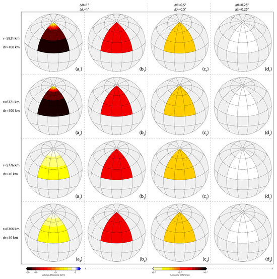
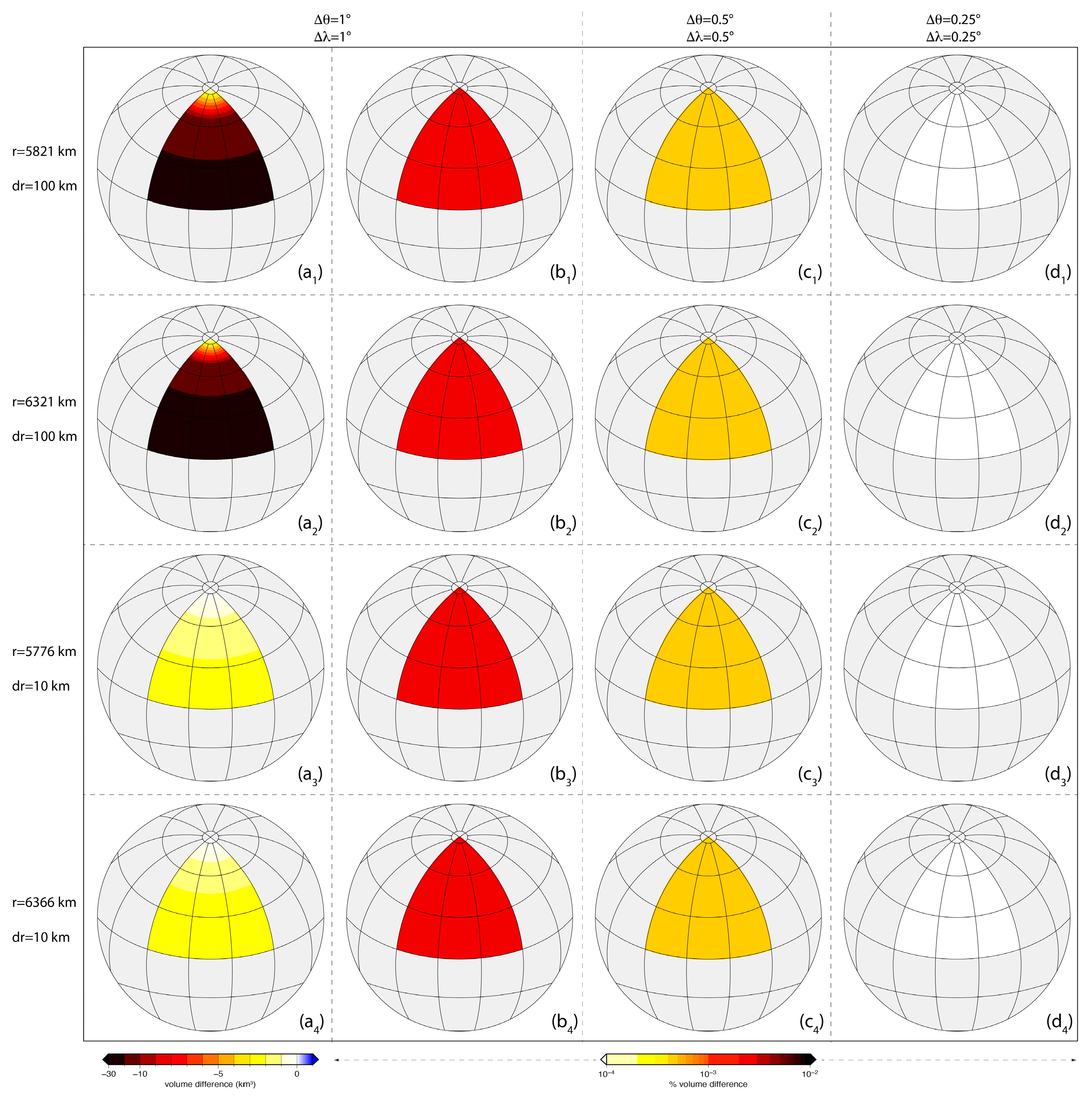
Figure 13 shows the volume difference and the percentage volume difference obtained for a spherical quadrangular prism, for different dimensions along the colatitude and the longitude (ranging from 1° to 0.25°) and along the radial direction (ranging from 100 km to 10 km for the real Earth, and to 1 km for the normalized Earth) using 125 Gauss–Legendre points.
Figure 13.
Values of volume differences (panels ai) and percentage volume differences (panels bi–di) for a spherical eight-node quadrangular right prism, for different distances r from the center of the spherical Earth, radial dr and angular and , along the colatitude and the longitude of the prism. A sphere with a radius of 6371 km is considered. In total, 125 Gauss–Legendre quadrature points are used.
There are two main results that are worthy of note.
- The volume difference decreases from tens of kilometers to a few units as the radial dimension of the spherical quadrangular spherical decreases (compare, in the first column, the first two panels at the top, with radial dimension of 100 km, with the two panels at the bottom, with radial dimension of 10 km), and decreases from the equator to the poles.
- Despite these differences in the volume difference related to r, however, the percentage volume difference is totally independent of r and of colatitude and longitude. It depends only on the angular dimension of the prism along the colatitude () and the longitude () and decreases as both decrease, from to lower than when and vary from to . A decrease in the percentage volume difference occurs when 27 Gauss–Legendre points are used, up to two orders of magnitude, but still below . The accuracy of the numerical estimation of the volume degrades significantly, instead, if only eight Gauss–Legendre points are used (Figure 14). The invariance of the percentage volume difference from the distance from the center of the sphere, as well as from the radial dimensions of the prism, is also confirmed by the results obtained for a normalized sphere (Figure 15).
Figure 14.
Values of volume differences (panels ai) and percentage volume differences (panels bi–di) for a spherical eight-node quadrangular right prism, for different angular dimensions and , along the colatitude and the longitude of the prism, for 8 and 27 Gauss–Legendre points. The distance of the prisms from the center of the sphere is r = 5776 km; their radial dimension is dr = 10 km. A sphere with a radius of 6371 km is considered.
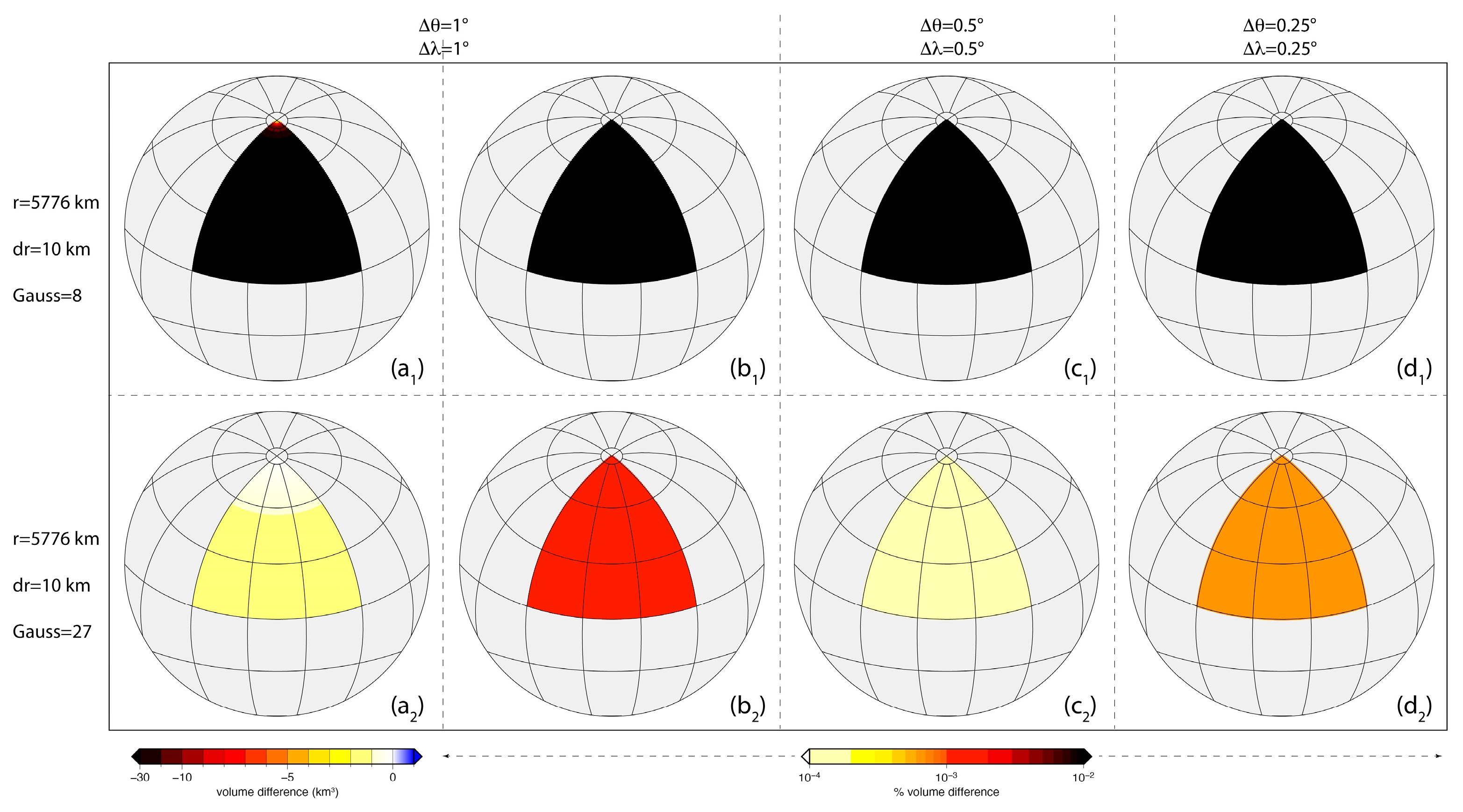
Figure 15.
Values of volume differences (a) and percentage volume differences (b–d) for a spherical eight-node quadrangular right prism, for different angular dimensions and , along the colatitude and the longitude of the prism, for 125 Gauss–Legendre points. The distance of the prisms from the center of the sphere is r = 1.5 km; their radial dimension is dr = 1 km. A sphere with a radius of 2 km is considered.
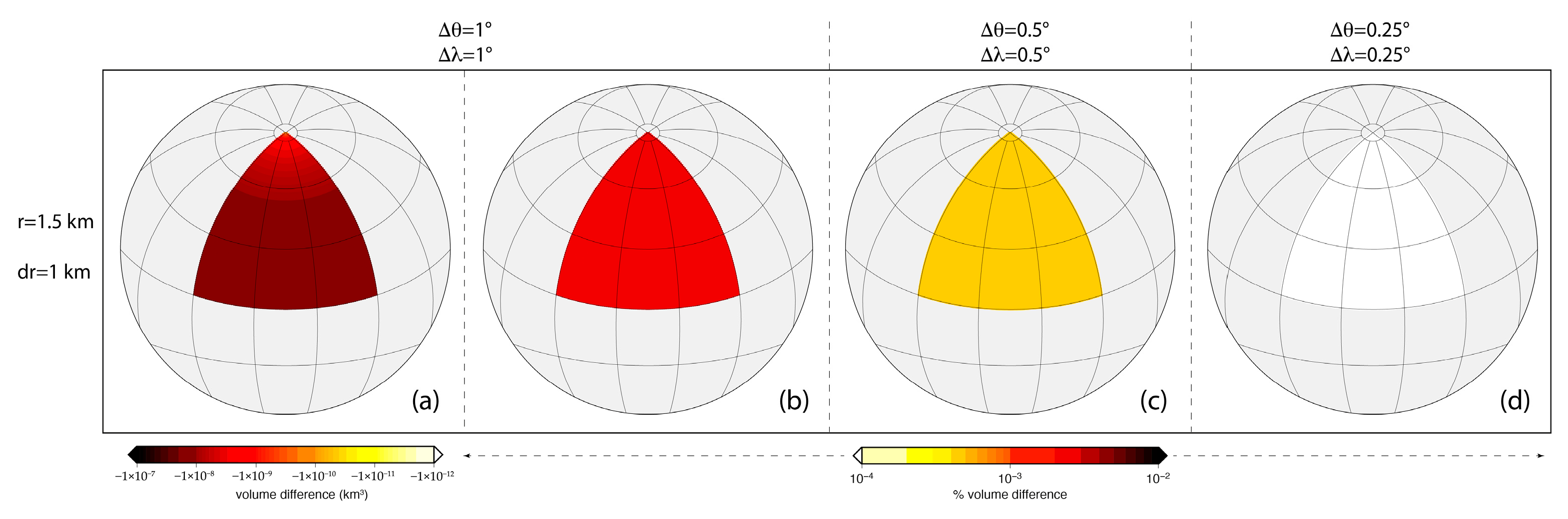
Figure 16 gives the results of an analysis similar to that performed for quadrangular spherical prisms, performed for a triangular spherical prism constructed on the same grid of points used to construct the quadrangular prisms in Figure 13, Figure 14 and Figure 15 and with two sides running along parallels and meridians.
Figure 16.
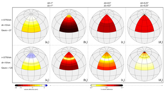
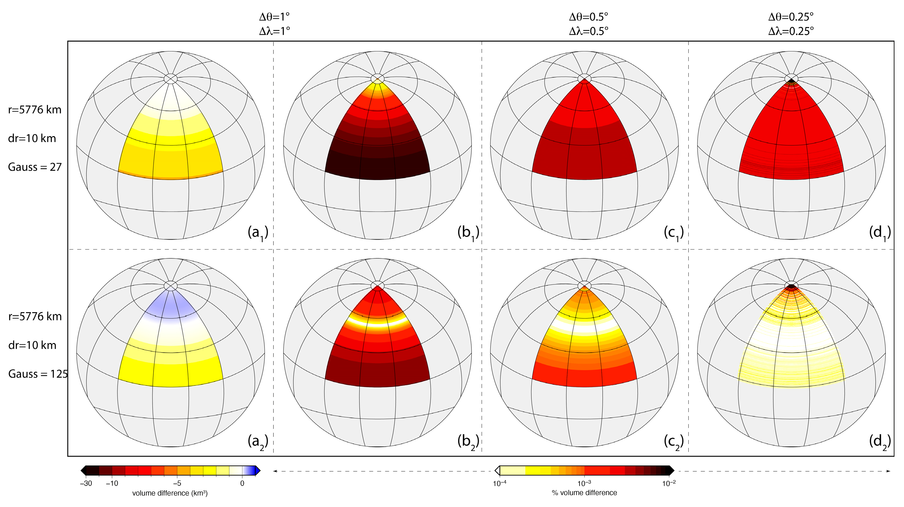
Values of volume differences (panels ai) and percentage volume differences (panels bi–di) for a spherical six-node triangular prism, for different angular dimensions and , along the colatitude and the longitude of the prism, for 27 (panels a1–d1) and 125 Gauss–Legendre points (panels a2–d2). The distance of the prisms from the center of the sphere is r = 5776 km; their radial dimension is dr = 10 km. A sphere with a radius of 6371 km is considered.
Both volume difference and percentage volume difference show different behavior from that of the spherical quadrangular prism. Specifically, while for a spherical quadrangular prism the numerical integral always underestimates the volume, in the case of a spherical triangular prism, the same occurs at lower latitudes and for few Gauss–Legendre quadrature points (panel a1), while at high latitudes and for many Gauss–Legendre quadrature points, the numerical integral is overestimated (panel a2), due to the coalescence of the Gauss points when the two upper sides of the triangular prisms become close when approaching the North Pole. Furthermore, the percentage volume difference for a spherical triangular prism varies with colatitude and reaches minimum values at middle latitudes. In the rest of the domain, the percentage volume difference remains at least one order of magnitude greater than those shown by the spherical quadrangular prism, but still below , with the sole exception occurring in proximity of the North Pole.
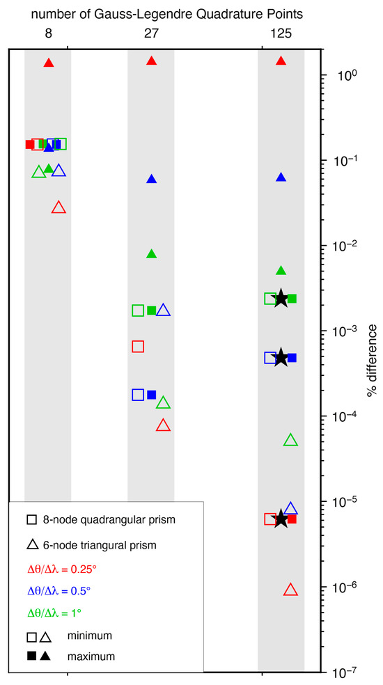
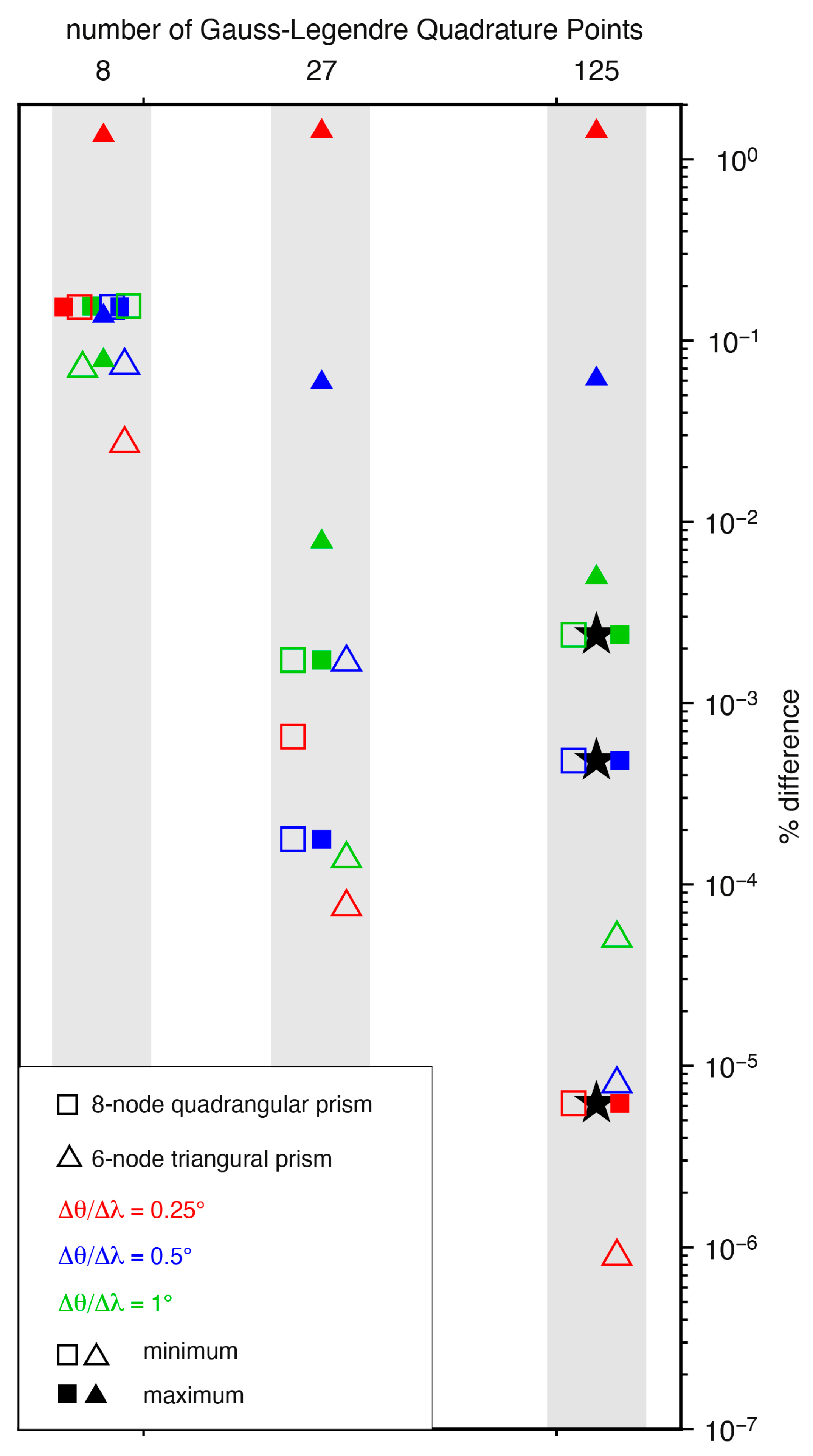
Figure 17 summarizes the results of the error variation analysis, expressed as the percentage difference between the numerically and analytically calculated volume, as a function of the number of Gauss–Legendre quadrature points for both models using six-node triangular prisms and those using eight-node quadrangular right prisms. This overall synthesized vision confirms the considerations made previously in the detailed discussion of some of the test models. It is worth emphasizing once again that, with the exception of the relatively high maximum percentage error (still less than 2%) that occurs only in the few spherical six-node triangular prisms facing the North Pole, the percentage error remains around 0.1% for eight Gauss–Legendre quadrature points, decreasing to 10−2 and 10−4 for 27 Gauss–Legendre quadrature points, and even as low as 10−6 for 125 Gauss–Legendre quadrature points.
Figure 17.
Variation of the error, in terms of maximum (solid symbols) and minimum (empty symbols) values of percentage difference between numerically and analytically computed volume, in function of the number of Gauss–Legendre quadrature points, for models using six-node triangular prisms (triangles) and eight-node quadrangular right prisms (squares). Different intervals of discretization have been used along the longitude (λ) and the colatitude (θ). The radial discretization is fixed at 10 km for all models except one, where it is 100 km (stars). Note that, for better clarity of the figure, for each order of quadrature, the symbols have been distributed within a horizontal band so as to avoid overlapping between them.
Furthermore, for eight Gauss–Legendre quadrature points, the variation of the percentage error remains smaller than one order of magnitude when different types of elements (six-node triangular and eight-node quadrangular prisms) and different discretizations in longitude and colatitude are used, around 0.1%; for higher orders of numerical integration, instead, the variation of the percentage error spans from three orders of magnitude (for 27 Gauss–Legendre quadrature points) to as many as five orders of magnitude (for 125 Gauss–Legendre quadrature points).
6.2. Steady-State Heat Conduction in a Sphere — Poisson and Laplace Problems
The second test is performed considering the numerical integration of the Poisson equation end comparing the numerical solution with specific analytical solutions of the same differential equation.
The Poisson equation has numerous applications in physics, such as in heat transfer, fluid dynamics, gravity field and electromagnetism. For our tests, we consider the equation for steady-state heat conduction in a sphere with internal heat production.
6.2.1. Numerical Integration of the Equation of Steady-State Heat Conduction in a Sphere with Internal Heat Production
The energy equation for steady-state heat conduction with internal heat production in spherical coordinates has the following expression:
where T is the temperature, is the thermal conductivity and is the internal energy per unit volume, with, in general, and functions of the position .
To proceed with the numerical integration, we use the Galerkin-weighted residual method. We herein synthetize the well-known mathematical formulation of the problem (e.g., ref. [14]), adapting the procedure to the spherical coordinates and proposed shape functions.
Let us consider the steady-state heat conduction problem defined, in compact form, by the following differential equation:
Let us assume the following boundary conditions:
with is the temperature prescribed on boundary and is the heat flow prescribed through the boundary .
The integral form of the problem is
where , and are generic continuous functions. Without loss of generality, we can assume and the integral form of the problem simplifies as
or, after integrating by part,
but
and the integral weak form of the problem takes the following form
Operatively, the evaluation of integral can be omitted by choosing function such that on . Furthermore, integral can be also omitted, since its result is easily handled during the resolution of the final system of algebraic equations. Finally, integral must be calculated only if a non-zero heat flow is assumed trough the boundary .
In conclusion, neglecting integrals , and , the integral weak form simplifies as
If the unknown T is approximated by the expression
where are the shape functions prescribed in terms of the independent variable and are the unknown temperatures at each of the grid nodes, and function is substituted by a set of prescribed functions in a number equal to the number of the unknown , and made to coincide with the shape functions (Galerkin approximation), the integral weak form becomes
or
with stiffness matrix, whose elements are
and load, whose elements are
In spherical coordinates the expression of the elements of the stiffness matrix becomes
To compute the volume integrals over the whole spherical volume , we summed the volume integrals computed over each spherical volume in which we discretized the continuum. We computed the elemental volume integrals numerically by means of the same Gauss–Legendre quadrature formula used for the validation test of the volume described in the previous sub-section. Since the unknown is a scalar, only the scalar component of the spherical shape functions has been considered, that is,
Numerical integration is performed on a spherical domain extending from the to , calculated from the center of a sphere of radius equal to . The longitude varies from 0 to 360° and the colatitude varies from 0 to 180°. A discretization varying from 5° to 1° is considered along both longitude and colatitude; a discretization of 5 and 10 km is assumed along the radial direction. Based on the results of the previous sub-section, we performed the numerical integration using eight Gauss–Legendre quadrature points.
6.2.2. Analytical Solution of the Equation of Steady-State Heat Conduction in a Sphere with Internal Heat Production
Let us consider again the energy equation for steady-state heat conduction with internal heat production in spherical coordinates
This differential equation has an exact solution only under certain simplifications.
Assume that thermal conductivity does not vary with . In this case, the differential equation becomes
or
which corresponds to the Poisson equation for temperature , with internal energy source and uniform conductivity . In absence of internal energy source, , the energy equation reduces to the Laplace equation for temperature .
Under spherical symmetry, with properties varying only in the radial direction, the solution of the Poisson equation can be expressed by spherical harmonics expansion
where are the spherical harmonics, of order m and degree l, and are the coefficients depending on the radial distance, which must be determined by solving the Poisson equation.
For our test, we assume the simple case of a temperature that varies only along the radial distance, , and the internal energy source is uniform. In this case, the Poisson equation reduces to
which can be integrated directly, obtaining the following general solution
with and integration constants to be determined after the application of appropriate boundary conditions.
We make use of Dirichlet boundary conditions:
After a few mathematical steps, we obtain the solution for temperature in the form of
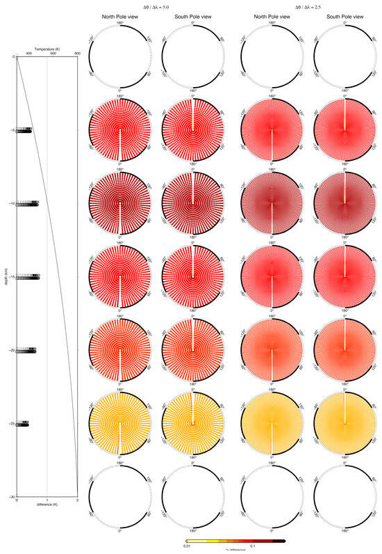
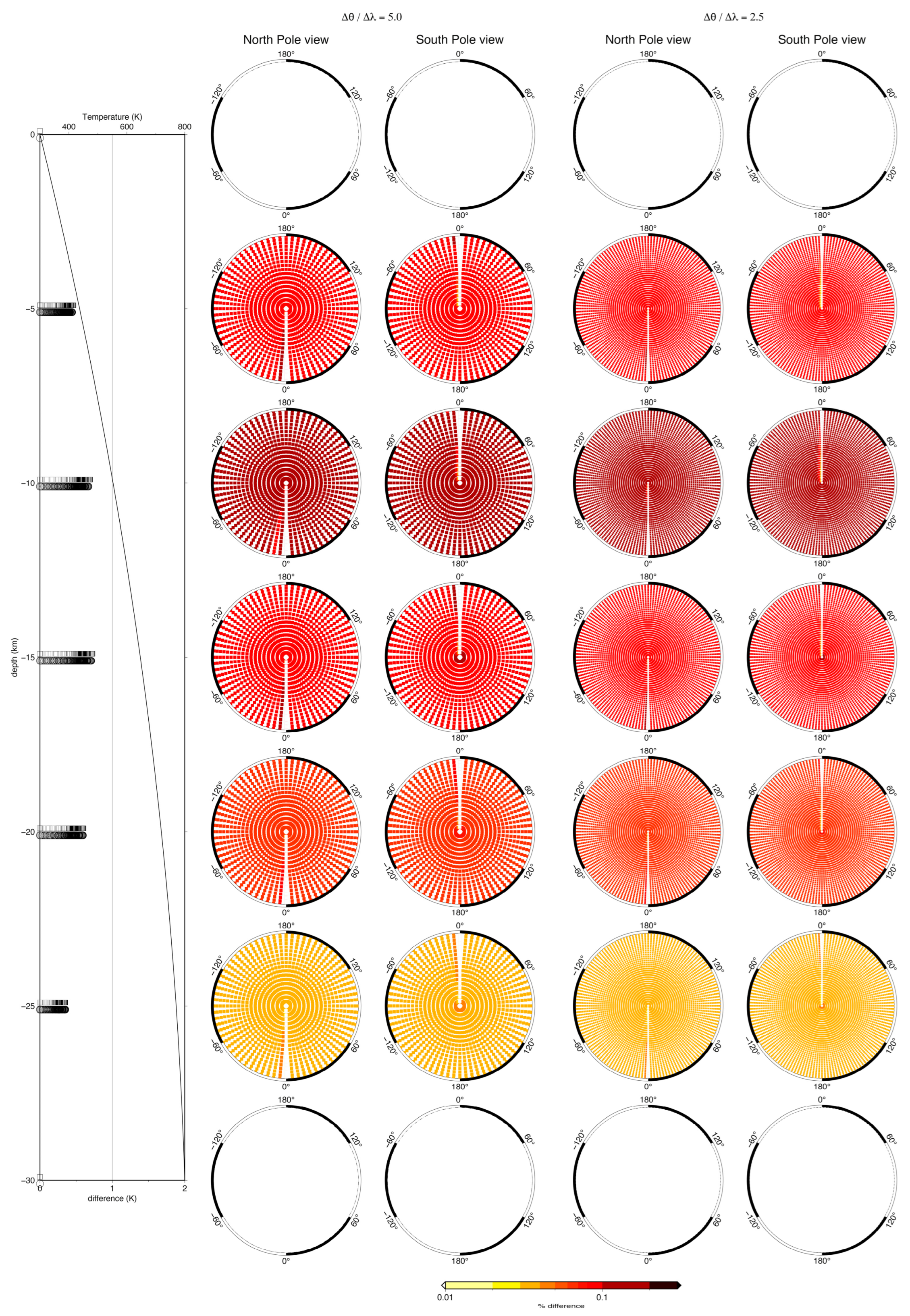
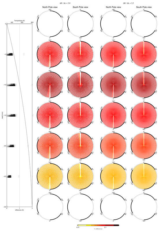
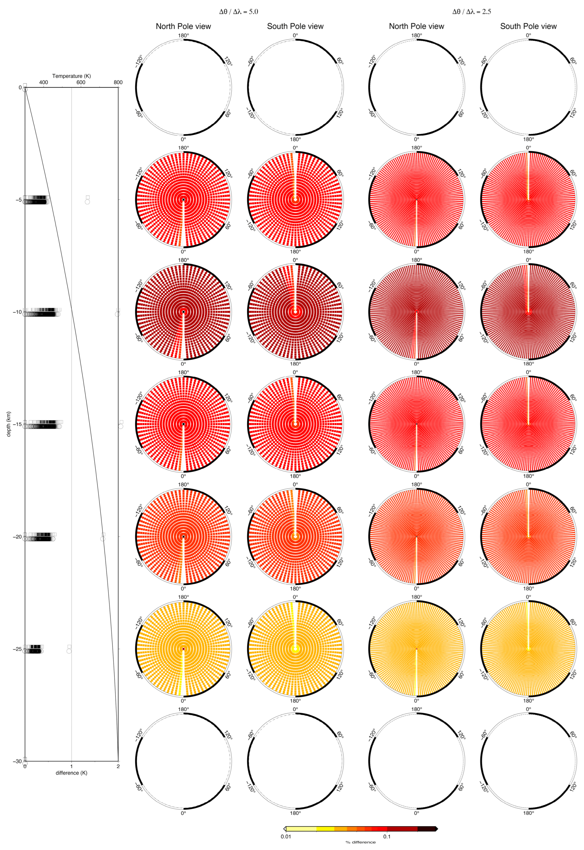
Figure 18 and Figure 19 show, for eight-node quadrangular right prisms and six-node triangular prisms, respectively, the comparison between the numerical and the analytical solutions, in terms of difference in temperature (left vertical panels) and percentage difference (circular panels), at different depths, from the base of the crust, at a 30 km depth, or , to the Earth’s surface, at , by 5 km stepping.
Figure 18.
Comparison between numerical and analytical solutions for eight-node quadratic right prisms, in terms of difference in temperature (black squares and circles in the left vertical panel) and percentage difference (circular maps), at different levels from the base of the crust, from 30 km depth (r = 6341 km), to the surface of the Earth (r = 6371 km). Different intervals of discretization have been used along the longitude and the colatitude, 5° (black squares in the left vertical panels and first and second columns on circular maps) and 2.5° (black circles in the left vertical panels and third and fourth columns on circular maps). The radial discretization is fixed at 10 km. Eight Gauss–Legendre quadrature nodes have been used. The solid line in the left vertical panel indicates the analytical solution.
Figure 19.
Comparison between numerical and analytical solutions for six-node triangular prisms, in terms of difference in temperature (black squares and circles in the left vertical panels) and percentage difference (circular maps), at different levels from the base of the crust, from a 30 km depth (r = 6341 km), to the surface of the Earth (r = 6371 km). Different intervals of discretization have been used along the longitude and the colatitude, 5° (black squares in the left vertical panels and first and second columns on circular maps) and 2.5° (black circles in the left vertical panel and third and fourth columns on circular maps). The radial discretization is fixed at 10 km. Eight Gauss–Legendre quadrature nodes have been used. The solid line in the left vertical panel indicates the analytical solution.
Unlike what was undertaken for the volume estimate (Section 6.1), for the present test, the numerical grid covers the whole sphere.
We assume , , and . In order to eliminate edge effects, along longitude 360° and colatitude 180°, the temperature is fixed to the analytical values. Based on the results in Section 6.1, n = 8 Gauss–Legendre quadrature points have been used.
The left panels of Figure 18 and Figure 19 contain a solid continuous line providing the analytical solution based on Equation (131), varying from 300 to 800 °K according to the prescribed Dirichlet boundary conditions and according to the temperature Kelvin degree scale at the top of the panels. The left panels contain also the difference in temperature between the analytical solution and the numerical solutions, provided by the black symbols at the different depths, including the spherical surfaces where the temperature matches the boundary conditions; for the symbols, the scale to be considered is the bottom one, from 0 to 2 °K. At the various depths, each black symbol is representative of each node of the numerical grid lying on the sphere at that depth; in the right circular panels, the same points are distributed spatially as a function of . The temperature difference varies from 0 °K to less than 1 °K for the eight-node quadrangular right prisms (Figure 18), with some increases at intermediate depths, as expected for the farthest distances from the fixed temperature boundary conditions. For the six-node triangular prisms (Figure 19) the temperature differences reach 2 °K, which are only encountered at the North Pole, at 10 and 15 km depths.
The four columns on the circular maps in Figure 18 and Figure 19 provide the percentage differences between the numerical solution and the analytical solution according to the bottom colored bar. Two different resolutions in latitude and longitude have been considered, 5° (first and second columns) and 2.5° (third and fourth columns), and the same depths as those for the vertical left panels are used. The first and third rows provide the North Pole perspective, and the second and fourth rows the South Pole perspective. Compared to the left vertical panels, these circular maps provide information on how differences between the numerical and analytical solutions are distributed over the spherical surfaces at the various depths. Only at 10 km depths, for both quadrangular and triangular prims, the percentage difference is slightly higher than 0.1%, with values that can be as low as 0.01% elsewhere. The white color in the top and bottom circular maps indicates that the boundary conditions are matched at the Earth’s surface and at the bottom of the crust; the white radii indicate at longitude 360° and colatitude 180°, matching with the analytical solution.
It is worth noting that the maximum percentage difference of 0.1 found in this test for the estimate of the temperature is of the same order of magnitude as that obtained for the volume estimate test (Section 6.1) for the same number of Gauss–Legendre quadrature points (eight).
Finally, even the relatively coarse grid () used is already capable of providing a satisfactory fit between numerical and analytical solutions. The maximum difference is in the order of 0.2% of the exact value, corresponding to a maximum difference of less than 1 °K for the absolute temperature, with the exception of the six-node triangular prism elements that show a maximum error, even if only at the North Pole, of about 2 °K (Figure 19).
7. Conclusions
We present the procedure to determine rigorous spherical shape functions for generic spherical prismatic elements and, in particular, for the case of spherical six-node tri-rectangular and eight-node quadrangular spherical prisms. The proposed analytical shape functions, as required, satisfy the properties of attaining the value one separately over each vertex, and smoothly reaching zero over all the remaining vertices. They also make it possible to interpolate a rigid displacement. We also derive the expression of the Jacobian. The results of numerical tests in which we compare the value of the exact volume of quadrangular and triangular spherical prisms and the value calculated numerically using the Jacobian formula containing the derivatives of the shape functions proposed here demonstrate the full capability of the presented spherical shape functions and the high degree of accuracy that can be achieved.
Our analytical shape functions make it possible to handle lateral variations in the physical properties of the Earth, thereby overcoming the limitation of spherical symmetry being required to solve global problems.
The proposed spherical shape functions can be used to rigorously interpolate scalar and vectoral fields within a spherical domain, which can be taken as reference elements within a finite element numerical code.
Author Contributions
Conceptualization, A.M.M., R.B. and R.S.; methodology, A.M.M., R.B. and R.S.; software, A.M.M.; validation, A.M.M., R.B. and R.S.; formal analysis, A.M.M., R.B. and R.S.; investigation, A.M.M., R.B. and R.S.; resources, A.M.M.; data curation, A.M.M., R.B. and R.S.; writing—original draft preparation, A.M.M., R.B. and R.S.; writing—review and editing, A.M.M., R.B. and R.S.; visualization, A.M.M.; supervision, A.M.M., R.B. and R.S.; project administration, A.M.M.; funding acquisition, A.M.M. All authors have read and agreed to the published version of the manuscript.
Funding
Research reported in this publication was supported by the ASI (Italian Space Agency)-funded project “NGGM/MAGIC-a breakthrough in the understanding of the dynamics of the Earth”, contr. n. CI-UOT-2023-057.
Data Availability Statement
The data generated and/or analyzed during this work are available from the corresponding author on reasonable request.
Acknowledgments
All figures have been made using GMT–The Generic Mapping Tools [16]. We thank the Editor and the reviewers for the valuable comments that helped us to improve the original manuscript.
Conflicts of Interest
The authors have no conflicts of interest to declare that are relevant to this work.
Appendix A. Partial Derivatives of for a Spherical Six-Node Tri-Rectangular Prism
References
- Schmeling, H.; Babeyko, A.; Enns, A.; Faccenna, C.; Funiciello, F.; Gerya, T.; Golabek, G.; Grigull, S.; Kaus, B.; Morra, G.; et al. A benchmark comparison of spontaneous subduction models—Towards a free surface. Phys. Earth Planet. Inter. 2008, 171, 198–223. [Google Scholar] [CrossRef] [Scilit]
- Moresi, L.; Quenette, S.; Lemiale, V.; Meériaux, C.; Appelbe, B.; Mühlhaus, H.-B. Computational approaches to studying non-linear dynamics of the crust and mantle. Phys. Earth Planet. Inter. 2007, 163, 69–82. [Google Scholar] [CrossRef] [Scilit]
- Moresi, L.; Dufour, F.; Mühlhaus, H.B. A Lagrangian integration point finite element method for large deformation modeling of viscoelastic geomaterials. J. Comput. Phys. 2003, 184, 476–497. [Google Scholar] [CrossRef] [Scilit]
- O’Neill, C.; Moresi, L.; Müller, D.; Albert, R.; Dufour, F. Ellipsis 3D: A particle-in-cell finite-element hybrid code for modelling mantle convection and lithospheric deformation. Comp. Geosci. 2006, 32, 1769–1779. [Google Scholar] [CrossRef] [Scilit]
- Braun, J.; Thieulot, C.; Fullsack, P.; DeKool, M.; Beaumont, C.; Huismans, R. DOUAR: A new three-dimensional creeping flow numerical model for the solution of geological problems. Phys. Earth Planet. Inter. 2008, 171, 76–91. [Google Scholar] [CrossRef] [Scilit]
- Popov, A.; Sobolev, S. SLIM3D: A tool for three-dimensional thermomechanical modelling of lithospheric deformation with elasto-visco-plastic rheology. Phys. Earth Planet. Inter. 2008, 171, 55–75. [Google Scholar] [CrossRef] [Scilit]
- Zhu, G.; Gerya, T.; Yuen, D.; Honda, S.; Yoshida, T.; Connolly, T. Three-dimensional dynamics of hydrous thermal-chemical plumes in oceanic subduction zones. Geochem. Geophy. Geosy. 2009, 118, 4682–4698. [Google Scholar] [CrossRef] [Scilit]
- Thieulot, C. FANTOM: Two- and three-dimensional numerical modelling of creeping flows for the solution of geological problems. Phys. Earth Planet. Inter. 2011, 188, 47–68. [Google Scholar] [CrossRef] [Scilit]
- Pusok, A.E.; Kaus, B.J.P. Development of topography in 3-D continental-collision models. Geochem. Geophys. Geosystems 2015, 16, 1378–1400. [Google Scholar] [CrossRef] [Scilit]
- Zhong, S.; Zuber, M.T.; Moresi, L.; Gurnis, M. Role of temperature-dependent viscosity and surface plates in spherical shell models of mantle convection. J. Geophys. Res. Solid Earth 2000, 105, 11063–11082. [Google Scholar] [CrossRef] [Scilit]
- Moresi, L.; Zhong, S.; Han, L.; Conrad, C.; Tan, E.; Gurnis, M.; Choi, E.; Thoutireddy, P.; Manea, V.; McNamara, A.; et al. CitcomS v3.3.1. Available online: https://zenodo.org/records/7271920 (accessed on 19 May 2025).
- Thieulot, C. ELEFANT: A user-friendly multipurpose geodynamics code. Solid Earth Discuss. 2014, 6, 1949–2096. [Google Scholar] [CrossRef] [Scilit]
- Bangerth, W.; Dannberg, J.; Fraters, M.; Gassmoeller, R.; Glerum, A.; Heister, T.; Myhill, R.; Naliboff, J. ASPECT: Advanced Solver for Problems in Earth’s ConvecTion, User Manual. Available online: https://figshare.com/articles/journal_contribution/ASPECT_Advanced_Solver_for_Problems_in_Earth_s_ConvecTion_User_Manual/4865333?file=51103820 (accessed on 19 May 2025).
- Zienkiewich, O.C.; Taylor, R.L. The Finite Element Method, Volume 1: The Basis; Butterworth-Heinemann: Oxford, UK, 2000. [Google Scholar]
- Cook, R.D.; David, S.M.; Michael, E.P. Concepts and Applications of Finite Element Analysis; Wiley: New York, NY, USA, 1989. [Google Scholar]
- Wessel, P.; Smith, W.H.F.; Scharroo, R.; Luis, J.F.; Wobbe, F. Generic Mapping Tools: Improved version released. Eos. Trans. AGU 2013, 94, 409–410. [Google Scholar] [CrossRef] [Scilit]
Disclaimer/Publisher’s Note: The statements, opinions and data contained in all publications are solely those of the individual author(s) and contributor(s) and not of MDPI and/or the editor(s). MDPI and/or the editor(s) disclaim responsibility for any injury to people or property resulting from any ideas, methods, instructions or products referred to in the content. |
© 2025 by the authors. Licensee MDPI, Basel, Switzerland. This article is an open access article distributed under the terms and conditions of the Creative Commons Attribution (CC BY) license (https://creativecommons.org/licenses/by/4.0/).