


Abstract
To improve the operational efficiency of the park source-load-storage system and reduce operation costs and the wind-solar curtailment rate, this paper establishes a Park Integrated Energy System (PIES) model with multiple energy storage and vehicle-to-grid (V2G) components and proposes an adaptive comprehensive fitness multi-objective particle swarm optimization algorithm. First, each component of the PIES is modeled. Second, electric vehicle (EV) scheduling boundaries, determined by wind and PV output, as well as a dynamic charging-discharging incentive mechanism, are designed to enhance renewable energy accommodation. Finally, an adaptive comprehensive fitness index is defined, and convergence and particle-update strategies are improved to achieve better scheduling performance. Simulation results verify that the proposed PIES model achieves optimal performance in terms of carbon-emission cost, total operation cost, and wind-solar curtailment rate. Meanwhile, the improved algorithm also outperforms traditional multi-objective methods in PIES scheduling.
1. Introduction
Faced with the increasingly severe challenges of global climate change and fossil energy depletion, the transition to a low-carbon, efficient, and sustainable energy system has become a global consensus and an inevitable trend of world energy development. As a key carrier of urban energy transition, the Park Integrated Energy System integrates electricity, heat, gas, and other energy forms to realize coordinated complementation and cascade utilization of various energies, playing an irreplaceable role in improving energy efficiency, promoting renewable energy consumption, and reducing carbon emissions [1].
With the rapid development of renewable energy technologies and the large-scale popularization of electric vehicles, integrating wind power (WP), photovoltaic (PV) power, and EVs into PIES has become an important development direction. As clean and renewable energy sources, wind and PV power have been widely used in PIES due to their environmental friendliness and abundant resources, effectively reducing the system’s dependence on fossil fuels and carbon emissions [2]. However, the inherent intermittency, randomness, and volatility of wind and solar output pose great challenges to the stable operation and optimal scheduling of PIES. With the increase in their penetration rate, renewable energy curtailment and low energy efficiency often occur [3]. Meanwhile, as flexible mobile energy storage units, EVs not only increase charging demand and the uncertainty of system load, but also can realize bidirectional energy interaction with the power grid through vehicle-to-grid technology, providing potential flexibility support for the optimal operation of PIES [4,5].
Optimal scheduling is the core technology to achieve safe, efficient, and low-carbon operation of the wind-solar-EV coupled system. In recent years, scholars have conducted relevant studies on the optimal scheduling of PIES. Ref. [6] proposed a bi-level optimization model based on multi-agent game theory, but ignored environmental benefits and the uncertainty of renewable energy. Ref. [7] incorporated carbon emission reduction targets into the scheduling model, but failed to fully consider the flexible regulation potential of EVs. Ref. [8] constructed an integrated energy system model of hydrogen storage and power generation considering alkaline electrolyzers and multiple operation modes, but did not involve EVs to enhance scheduling flexibility. Ref. [9] proposed a grid-independent park-level integrated energy system with hydrogen storage, using wind, solar, and natural gas as main energy supplies to replace fossil fuels, but did not consider the coupling characteristics between wind-solar energy and EVs. Ref. [10] established an optimal operation model of PIES based on a robust algorithm and adaptive genetic algorithm, but did not consider multi-objective collaborative optimization. Ref. [11] studied a wind-solar-gas complementary integrated energy system for combined cooling, heating, and power supply in an agricultural park, but did not consider the coordination of multiple energy storage. Ref. [12] combined electricity and carbon quota trading to establish a direct electricity-carbon trading mechanism for high-economic-efficiency IES (integrated energy system) operation, yet the multi-energy complementation mechanism still needs improvement. Ref. [13] proposed a grid-connected IES considering the complementation of geothermal and solar energy with thermal storage, but did not exploit the scheduling potential of EVs. Ref. [14] established a Stackelberg game model between the integrated energy system operator and IES, but there is still room for improvement in renewable energy accommodation.
In addition, existing multi-objective scheduling models often have defects in balancing conflicting objectives, and solution methods struggle to obtain uniformly distributed Pareto optimal solutions, which cannot fully meet the actual operation requirements of PIES under wind-solar-EV coupling [15,16]. Ref. [17] established an improved IES scheduling optimization model based on modified particle swarm optimization, but only took daily operating cost as the objective function without multi-objective coordination. Ref. [18] combined non-dominated sorting genetic algorithm II (NSGA-II) and beluga whale optimization (BWO) to solve the model optimization problem, but did not achieve a collaborative multi-objective optimum.
In summary, existing studies have achieved abundant results but still have deficiencies: most studies fail to effectively couple wind-solar output with the charging-discharging behavior of electric vehicles, lacking dynamic coupling and incentive mechanisms, so the scheduling potential needs to be improved; existing scheduling algorithms struggle to coordinate objectives such as low-carbon performance, economic efficiency and wind-solar curtailment rate, making multi-objective scheduling difficult and leading to increased operating costs or higher carbon emission costs. To address the above problems, this study proposes a multi-objective collaborative optimization method for PIES based on the Adaptive Weight Comprehensive Fitness Multi-Objective Particle Swarm Optimization (AWCF-MOPSO) algorithm, constructs a PIES model coupled with wind power, photovoltaic power, and electric vehicles, and verifies the effectiveness of the method through multi-scheme comparative simulation experiments.
2. Modeling of Wind-Solar-EV Coupled PIES
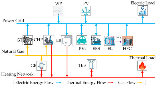
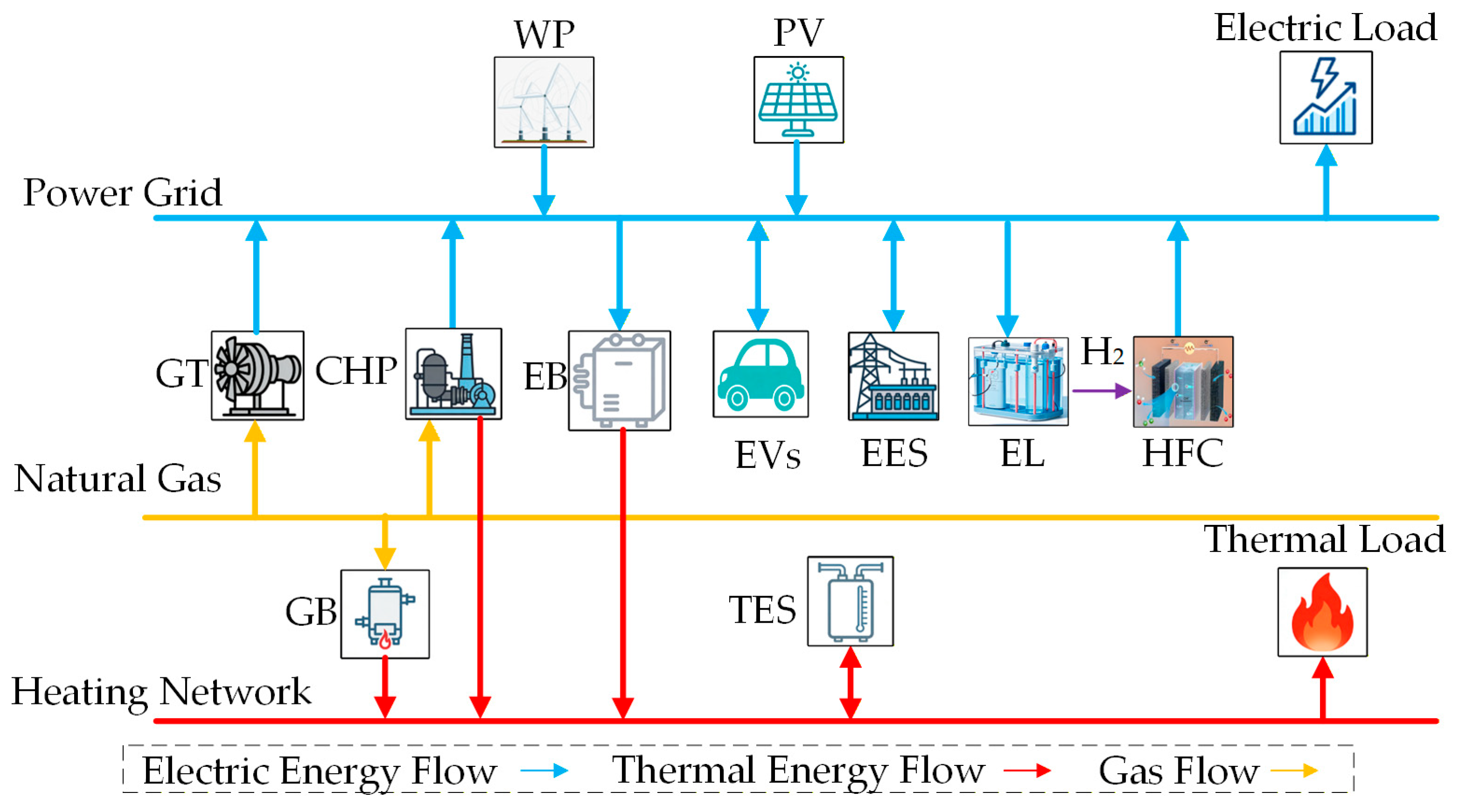
The PIES operation framework constructed in this paper is shown in Figure 1, which mainly consists of an energy supply unit, an energy coupling unit, an energy storage unit, and an energy consumption unit. The energy supply unit includes on-site wind power, on-site photovoltaic power, the utility grid, utility gas network and natural gas; the energy coupling unit includes combined heat and power (CHP) units, gas turbines (GT), gas boilers (GB), electrical boilers (EB), electrolyzers (EL) and hydrogen fuel cells (HFC); the energy storage unit includes electrical energy storage (EES), thermal energy storage (TES) and electric vehicles; and the energy consumption unit includes electric loads and thermal loads.
Figure 1.
Structure of the integrated energy system.
2.1. Basic Equipment Model of PIES
2.1.1. CHP
The mathematical model of CHP is expressed as follows:
where is the electric power output by CHP at time ; is the power generation efficiency of CHP; is the natural gas consumption of CHP at time ; is the low calorific value of natural gas; is the thermal power output by CHP at time ; is the heat production efficiency of CHP; is a 0–1 variable indicating whether CHP operates at time (0 = OFF, 1 = ON); and are the lower and upper limits of natural gas input to CHP, respectively; and are the lower and upper ramp limits of CHP, respectively.
2.1.2. GT
The mathematical model of GT can be expressed as follows:
where is the electric power output by GT at time ; is the power generation efficiency of GT; is the natural gas consumption of GT at time ; is a 0–1 variable indicating whether GT operates at time ; and are the lower and upper limits of natural gas input to GT, respectively; and are the lower and upper ramp limits of GT, respectively.
2.1.3. GB
The mathematical model of GB can be expressed as follows:
where is the thermal power output by GB at time ; is the heat production efficiency of GB; is the natural gas consumption of GB at time ; is a 0–1 variable indicating the operation status of GB at time ; and are the lower and upper limits of natural gas input to GB, respectively.
2.1.4. EB
The mathematical model of EB can be expressed as follows:
where is the thermal power output by EB at time ; is the heat production efficiency of EB; is the electric power consumption of EB at time ; is a 0–1 variable indicating the operation status of EB at time ; and are the lower and upper limits of electric power input to EB, respectively.
2.1.5. EES
The mathematical model of EES can be expressed as follows:
where is the stored energy of EES at time ; is the self-discharge rate of EES; and are the charging and discharging power of EES at time , respectively; and are the charging and discharging efficiency of EES, respectively; is the time interval; and are 0–1 variables indicating the charging and discharging status of EES, respectively; and are the peak charging and discharging power of EES, respectively; and are the lower and upper capacity limits of EES, respectively.
2.1.6. TES
The mathematical model of TES can be expressed as follows:
where is the stored heat of TES at time ; is the self-heat release rate of TES; and are the heat storage and release rate of TES at time , respectively; and are the heat storage and release efficiency of TES, respectively; and are 0–1 variables indicating the heat storage and release status of TES, respectively; and are the peak heat storage and release rate of TES, respectively; and are the lower and upper heat storage capacity limits of TES, respectively.
2.1.7. EL
The mathematical model of EL can be expressed as follows:
where is the hydrogen production mass flow rate of EL at time ; is the power generation efficiency of EL; is the electric power consumption of EL at time ; is the low calorific value of hydrogen; is a 0–1 variable indicating whether EL operates at time ; and are the lower and upper limits of electric power input to EL, respectively; and are the lower and upper ramp limits of EL, respectively.
2.1.8. HFC
The mathematical model of HFC can be expressed as follows:
where is the power generation of HFC; is the power generation efficiency coefficient of HFC; is the recovered heat of HFC; is the waste heat recovery coefficient of HFC; is the maximum power generation of HFC.
2.2. Wind-Solar-EV Coupling Model
The charging-discharging behavior of EV can be expressed as:
where is the power of the i-th EV; and are the charging and discharging power of the i-th EV, respectively; and are 0–1 variables indicating the charging and discharging status of EV, respectively; and are the allowable maximum charging and discharging power of the i-th EV, respectively.
The battery state of charge (SOC) model of EV is as follows:
where is the state of charge of the i-th EV; and are the charging and discharging efficiency of EV, respectively; is the battery capacity of the i-th EV.
Since vehicles are only included in the total power when connected to the grid, for a cluster of electric vehicles, its model is:
where is the total power of the electric vehicle cluster; and are the charging-discharging power limits of the charging pile cluster; and are the access and departure times of the i-th EV, respectively.
The probability density function of vehicle access time is as follows:
where and are the standard deviation and expectation of EV access time, respectively; and are the standard deviation and expectation of EV departure time, respectively.
To prevent battery life damage caused by excessive pursuit of accommodation and user travel failure due to excessive scheduling, the following constraints are added to the EV SOC:
where is the minimum allowable SOC of EV; is the maximum allowable SOC of an electric vehicle; is the minimum SOC required for the i-th EV when leaving.
The coupled charging-discharging power scheduling model is as follows:
where and are the wind power and photovoltaic output, respectively; and are the installed capacities of wind power and photovoltaic, respectively; is the system wind-solar adequacy coefficient; is the EV power consumption coefficient; and are the rated upper and lower limits of charging-discharging power of the i-th EV, respectively.
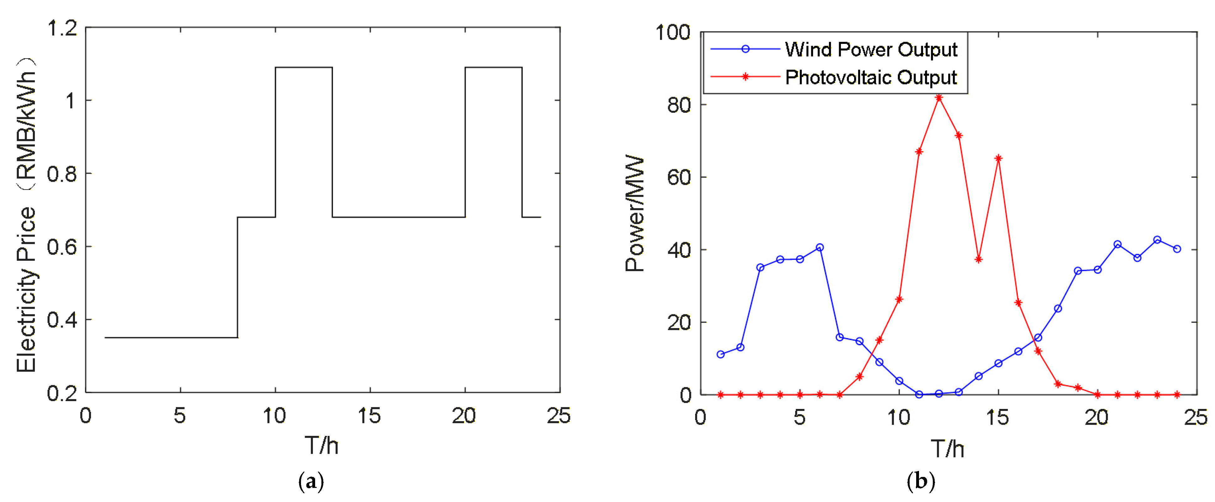
In this study, the output data of wind turbines and photovoltaic units are treated as known conditions, which are derived from the wind generators and photovoltaic panels installed within an industrial park in China. The upper limit of EV charging-discharging power is determined by wind-solar output data and the current total power of the EV cluster, realizing the scheduling logic that the greater the wind-solar output, the higher the charging priority. The wind-solar adequacy coefficient and EV power consumption coefficient are defined to adjust the allowable charging-discharging power of a single EV. When the wind-solar adequacy coefficient is larger and the EV power consumption coefficient is smaller, the allowable maximum charging power of EV will be relaxed, while the allowable maximum discharging power of EV will be narrowed; on the contrary, when the wind-solar adequacy coefficient is smaller and the EV power consumption coefficient is larger, the allowable maximum charging power of EV will be narrowed, while the allowable maximum discharging power of EV will be relaxed.
To solve the problems of low willingness of EV V2G discharging and insufficient initiative to respond to scheduling, a differentiated discharging incentive model coupled with wind-solar output deficit is constructed. Based on time-of-use (TOU) electricity price, wind-solar deficit coefficient, and EV power consumption coefficient, the real-time discharging incentive unit price is determined to ensure that the incentive unit price is higher than the conventional charging electricity price and lower than the grid TOU power purchase price, balancing the park’s economic cost and EV owner benefits. The mathematical expression is:
where is the discharging incentive unit price of the electric vehicle at time t; is the grid TOU power purchase price at time t; is the incentive adjustment coefficient; is the incentive trigger coefficient.
To ensure that the incentive mechanism is compliant and in line with engineering practice, the following incentive constraints are set to avoid excessive incentive cost or disordered discharging and limit the incentive price:
where is the grid peak electricity price.
3. Improved Design of AWCF-MOPSO Algorithm
3.1. Multi-Objective Particle Swarm Optimization Algorithm
The core feature of a multi-objective optimization problem (MOP) is that there are multiple conflicting objective functions, and there is no unique global optimal solution, but only a set of non-dominated solutions (Pareto optimal solutions); that is, it is impossible to improve the performance of one objective without reducing the performance of other objectives. The low-carbon optimal scheduling of PIES involves multiple objectives, such as carbon emissions and operation cost, so the multi-objective particle swarm optimization (MOPSO) algorithm needs to be introduced. Based on the traditional PSO, the MOPSO algorithm extends to the field of multi-objective optimization by introducing mechanisms such as non-dominated sorting and external archive. Its core is to search for a uniform, diverse Pareto-optimal solution set through particle iteration.
Firstly, the multi-objective optimization problem of PIES low-carbon optimal scheduling can be uniformly described as:
where is the decision variable vector; is the multi-objective function vector; ∼ are each independent objective function; is the j-th inequality constraint; is the l-th equality constraint; and are the lower and upper limits of the decision variable, respectively.
For the above multi-objective optimization problem, non-dominated solutions and a Pareto-optimal solution set are defined.
Non-dominated solution: For two feasible solutions and , if “for all objective functions, ( = 1, 2, …, ), and there is at least one objective function such that ”, then dominates ; if no feasible solution can dominate , then is a non-dominated solution.
Pareto optimal solution set: The set of all non-dominated solutions, denoted as where X is the feasible solution space; the set of objective function values corresponding to the Pareto-optimal solution set is called the Pareto front.
An external archive is set to store all non-dominated solutions generated during the iteration and eliminate dominated particles. When the capacity of the external archive exceeds the preset value, particles with smaller crowding distances are sorted out to maintain particle diversity and avoid local concentration of the Pareto front. The crowding distance of the i-th particle is calculated as follows:
where and are the values of the (i + 1)-th and (i − 1)-th particles on the m-th objective function (sorted in ascending order of the objective function value); and are the maximum and minimum values of the m-th objective function in the external archive, respectively.
3.2. Setting of Low-Carbon Preference Optimal Scheduling Objective Function
In multi-objective optimization, the traditional single-objective fitness cannot balance the trade-off relationship between multiple objectives, and the fitness calculation relies on fixed weights, making it difficult to achieve dynamic adjustment. Unlike traditional MOPSO with fixed weights, we design a low-carbon preference adaptive weight adjustment strategy that dynamically updates the weights of carbon emission cost, operation cost, and wind-solar curtailment rate according to real-time system status, solving the problem of unbalanced multi-objective coordination.
3.2.1. Low-Carbon Objective: Minimizing Total System Carbon Emissions
The total system carbon emissions mainly come from fossil energy power generation and from carbon emissions of energy conversion equipment. The carbon emission coefficient is introduced to quantify carbon emissions into carbon cost. The objective function expression is:
where is the total system carbon emissions; is the scheduling period; is the number of fossil energy power generation equipment; is the carbon emission cost coefficient of the i-th fossil energy power generation equipment; is the output of the i-th fossil energy power generation equipment at time t; is the number of energy conversion equipment; is the carbon emission cost coefficient of the j-th energy conversion equipment; is the input power of the j-th energy conversion equipment at time t.
3.2.2. Economic Objective: Minimizing Total System Operation Cost
The total system operation cost includes fossil energy procurement costs, renewable energy curtailment loss, energy storage equipment operation and maintenance (O&M) costs, and grid interaction costs. The objective function expression is:
where is the total system operation cost; is the energy procurement cost coefficient of the i-th fossil energy power generation equipment; is the curtailment loss coefficient of the k-th renewable energy power generation equipment; is the curtailment power of the k-th renewable energy power generation equipment at time t; is the number of energy storage equipment; is the O&M cost coefficient of the l-th energy storage equipment; is the charging-discharging power of the l-th energy storage equipment at time t; is the grid interaction power at time t.
3.2.3. Efficiency Objective: Minimizing System Wind-Solar Curtailment Rate
The wind-solar curtailment rate is a core indicator measuring the renewable energy accommodation efficiency. Minimizing the wind-solar curtailment rate can improve energy utilization efficiency. The objective function expression is:
where is the system wind-solar curtailment rate, the wind-solar curtailment rate is the ratio of unaccommodated wind-solar power to total wind-solar generation; is the predicted output of the k-th renewable energy power generation equipment at time t.
3.2.4. Adaptive Weight Comprehensive Fitness Design
The Adaptive Weight Comprehensive Fitness index is introduced as the criterion for judging the quality of particles. The personal best is updated if the comprehensive fitness of the current particle is better than that of its individual best particle, or if they have the same non-dominated rank but the current particle yields higher comprehensive fitness. Moreover, comprehensive fitness can assist in the selection of the global best particle. The particle with the optimal comprehensive fitness is selected from the external archive as the global best particle, guiding the whole particle swarm to iterate toward the multi-objective collaborative optimum and ensuring that the optimization results match the low-carbon preference and the system operating status.
As the three objective functions have different dimensions, direct weight assignment is not applicable. Therefore, the objective functions need to be standardized first and mapped to the interval [0, 1] to eliminate dimensional influences. A linear standardization method is adopted, and the standardization formula is given as follows:
where is the normalized value of the k-th objective function; is the minimum value of the k-th objective function; is the maximum value of the k-th objective function.
The weight calculation method for the three objective functions is as follows:
where , , and are the weights of the three objective functions, respectively; is the low-carbon preference coefficient, which is set to 0.5 in this paper; and are the normalized values of the economic objective and efficiency objective, respectively.
When the system carbon emission is excessively high, is increased while and are decreased, giving priority to the low-carbon objective. When the system operation cost is excessively high, is increased and is moderately reduced. When the wind-solar curtailment rate of the system is excessively high, is increased and is moderately reduced, prioritizing the improvements of renewable energy accommodation efficiency. When the system operates in a stable state, the weights remain stable to achieve multi-objective collaborative optimization.
Combined with the standardized objective function values, the adaptive weight comprehensive fitness of each particle is obtained via weighted summation, and the formula is given as follows:
where represents the comprehensive fitness of the i-th particle.
3.3. Improvement of Convergence Performance and Particle Update
We replace the fixed inertia weight with a linearly decreasing inertia weight combined with random disturbance, which balances the global search ability in the early iteration and local convergence ability in the late iteration, effectively avoiding falling into a local optimum. The formula is:
where is the inertia weight of the t-th iteration; and are the maximum and minimum inertia weight, set to 0.9 and 0.4 in this study; is the maximum number of iterations, set to 150 in this study; is the random disturbance coefficient, set to 0.01 in this study; is a random number in the interval [0, 1], used to increase the randomness of inertia weight and avoid the algorithm falling into local optimum.
To further improve the diversity and optimality of the Pareto-optimal solution set, a particle update strategy combining elite retention and random mutation is introduced.
- Elite retention: After each iteration, the top 20% elite particles with the largest crowding distance in the external archive are directly retained for the next iteration to ensure that high-quality solutions are not lost.
- Random mutation: Random mutation is performed on particles trapped in a local optimum (particles with no position change for 5 consecutive iterations in this study). The mutation formula is:
4. Discussion
To verify the rationality of the optimal scheduling model for the wind-solar-EV coupled PIES under weather impacts constructed in this paper, as well as the solving performance of the proposed improved multi-objective particle swarm optimization algorithm, this section carries out a multi-scenario simulation analysis based on the system mathematical model, the improved multi-objective optimization algorithm, and the various constraints mentioned above, using a typical operation scenario of a PIES in China.
4.1. Establishment of Objective Functions
4.1.1. Carbon Emission Cost
In the park-integrated energy system presented in this paper, the carbon-emission accounting boundary includes direct and indirect carbon emissions. Direct carbon emissions come from the power generation and energy conversion processes of CHP, GT, GB and other equipment, which need to be calculated according to fuel consumption (converted into electric and thermal power for easy calculation). Indirect carbon emissions come from the carbon emissions of purchased electricity and heat, which need to be calculated according to the amount of energy purchased from the power grid and heat grid. The carbon emission cost objective function is as follows:
where , , , and are the carbon emission cost factors of CHP, GT, GB, purchased electricity, and purchased heat, respectively; and are the electricity and heat purchased from the grid side at time t, respectively.
4.1.2. Total System Operation Cost
The total operation cost generated during the operation of the PIES system in this paper includes grid power purchase cost, fossil energy procurement cost, heat purchase cost, renewable energy curtailment cost, energy storage equipment O&M cost, EV discharging cost, EV discharging incentive, and EV charging revenue is considered. The objective function is as follows:
where , , , , , and are the grid power purchase cost coefficient (TOU price), fossil energy procurement cost coefficient, heat purchase cost coefficient, wind curtailment cost coefficient, photovoltaic curtailment cost coefficient, EV discharging cost coefficient, and EV charging revenue coefficient, respectively; , and are the electric power, natural gas, and thermal power purchased by the park at time t, respectively; and are the O&M cost coefficients of EES and TES, respectively; is the start-stop cost of the i-th equipment; is the start-stop status of the i-th equipment.
4.1.3. System Wind-Solar Curtailment Rate
The system wind-solar curtailment rate is a core indicator measuring the level of renewable energy accommodation. The calculation formula is as follows:
where and represent the curtailed power of wind power and photovoltaic systems at time t, respectively; is the total wind-solar output power at time t, which equals the sum of and .
4.2. Establishment of Constraints
The constraints in this paper include the electric power supply-demand balance constraint, thermal power supply-demand balance constraint, natural gas supply-demand balance constraint, etc.
4.2.1. Electric Power Balance Constraint
4.2.2. Thermal Power Supply Demand Balance Constraint
4.2.3. Natural Gas Supply Demand Balance Constraint
4.3. Experimental Parameter Setting
To verify the effectiveness of the proposed low-carbon optimization solution method, three schemes are designed for the comparative simulation of intra-day rolling optimal scheduling. Scheme 1: Only the electric vehicle charging model is considered. Scheme 2: The electric vehicle charging and discharging model is considered. Scheme 3: The wind-solar and electric vehicle coupling model is considered. There are 100 electric vehicles in total, with a maximum total charging power of 30 MW and a maximum total discharging power of 10 MW. The remaining parameter configurations are listed in the Appendix A.
4.4. Scheduling Result Analysis
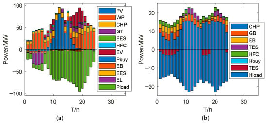
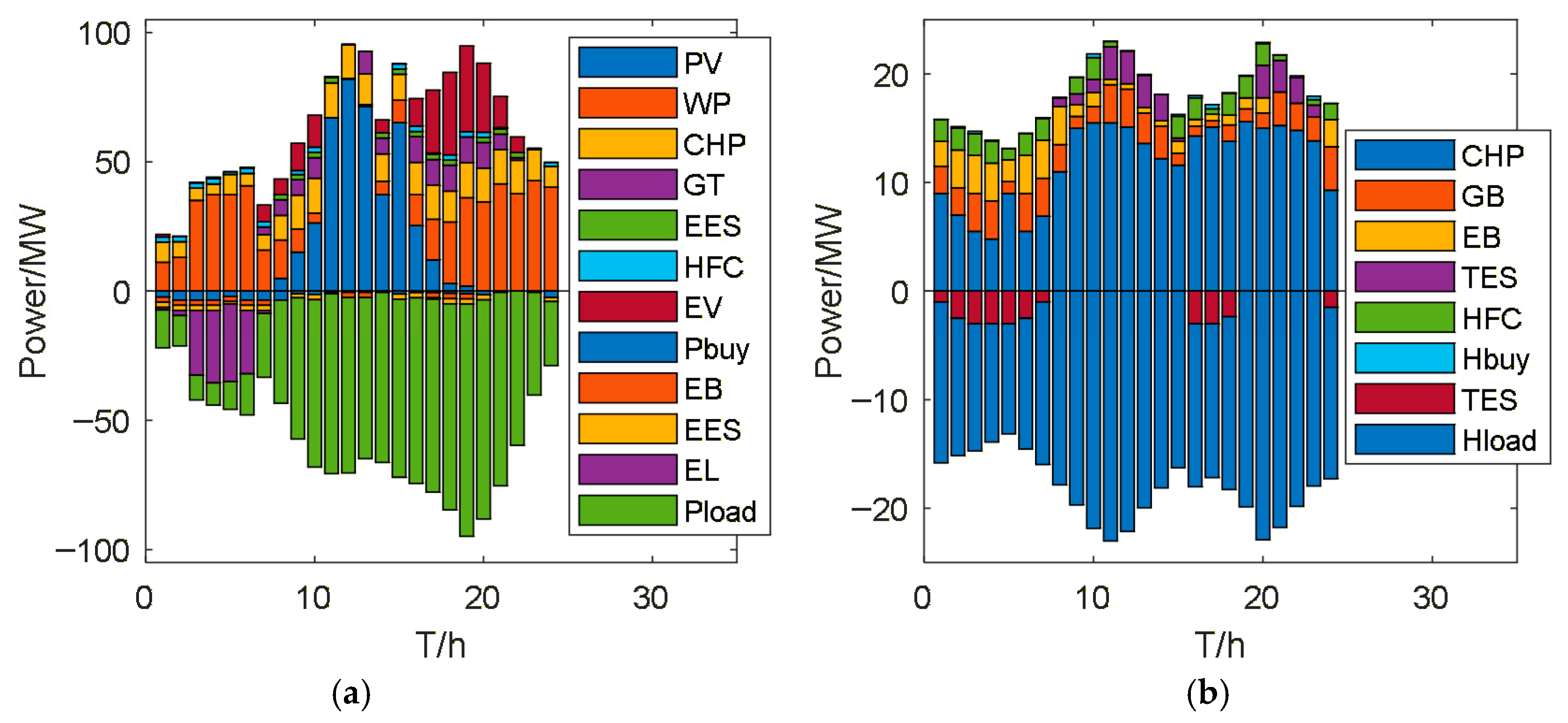
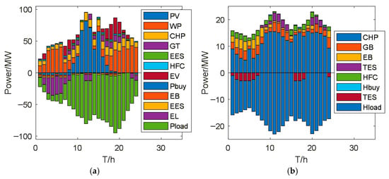
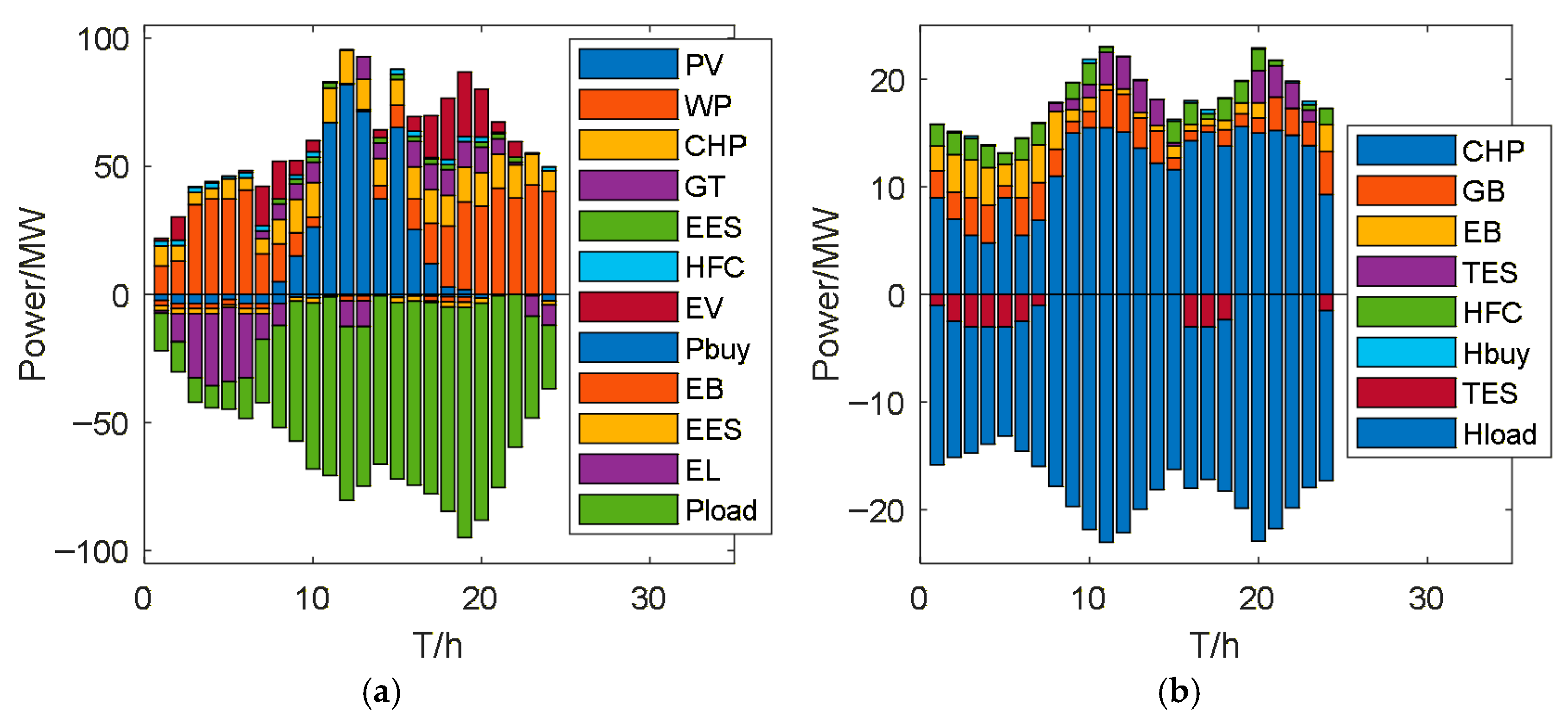
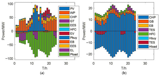
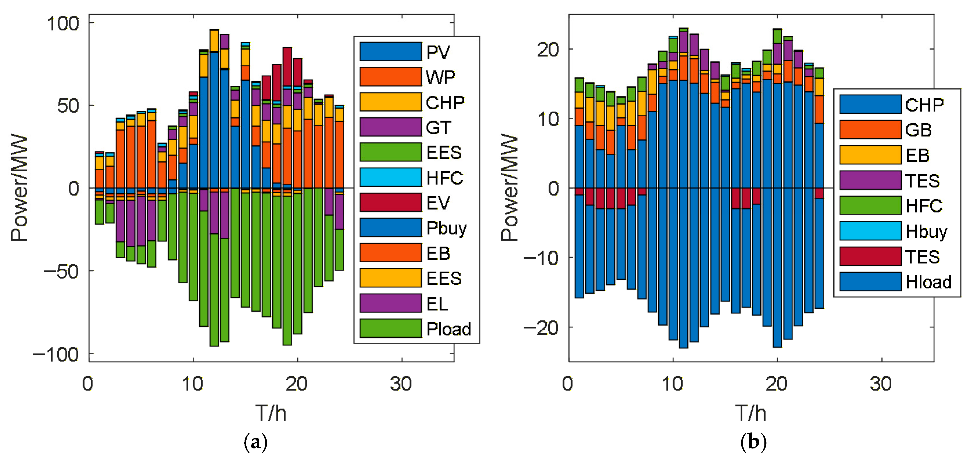
The comparative analysis results for the three optimal scheduling schemes show that Scheme 3 has the best comprehensive performance, Scheme 2 is the second, and Scheme 1 has the worst effect, as shown in Figure 2, Figure 3 and Figure 4. In all figures, energy sources are plotted on the positive y-axis, and loads are plotted on the negative y-axis. When the energy storage is on the positive y-axis, it indicates that it is in the energy release state; when it is on the negative y-axis, it indicates that it is in the energy storage state.
Figure 2.
(a) Electric Power Balance of Scheme 1; (b) Thermal Power Balance of Scheme 1.
Figure 3.
(a) Electric Power Balance of Scheme 2; (b) Thermal Power Balance of Scheme 2.
Figure 4.
(a) Electric Power Balance of Scheme 3; (b) Thermal Power Balance of Scheme 3.
The optimal scheduling results of the three schemes are analyzed and compared by dividing the entire day into four periods, in combination with the electric–thermal load balance diagrams, electricity price profiles, and thermal load characteristics.
The period of 1–6 h is the valley-load stage with an initially rising wind and photovoltaic output. During this interval, the electric load ranges from 8.6 MW to 14.7 MW, and the thermal load is 13.2–16.0 MW. There is no photovoltaic output, while wind power output climbs gradually from 11.1 MW to 37.4 MW. On the power side, Scheme 3 prioritizes wind power accommodation with energy storage and residual loads: the electric boiler operates steadily at 2.3–3.5 MW, the electric energy storage is fully charged, the electric load remains at 1.1–2.0 MW, and the purchased power is the lowest during this period. Scheme 2 realizes regulation through the charging and discharging of electric vehicles, with lower purchased power and wind-photovoltaic curtailment than Scheme 1. However, it fails to consider the coupling between electric vehicles and wind-photovoltaic resources, so its wind and photovoltaic curtailment remains higher than that of Scheme 3 in the absence of charging and discharging incentives. In Scheme 1, electric vehicles only operate in the charging mode without discharge support, resulting in insufficient utilization of energy storage and adjustable equipment, as well as the highest purchased power and wind curtailment. On the thermal side, the three schemes exhibit a consistent changing trend, focusing on thermal energy storage reserve and cost control. The combined heat and power unit produces heat at 4.8–9.0 MW; the gas boiler supplies energy at 2.5–3.5 MW, thermal storage is charged at 1.0–2.5 MW; and the purchased heat is merely 0.02–0.11 MW. Economic logic: Grid electricity prices are at the valley level, and wind power has a surplus. Physical mechanism: EVs and EES are charged preferentially to store surplus wind energy, reducing wind curtailment and avoiding high-cost peak electricity purchase later.
The period of 7–12 h witnesses continuous load growth and the peak of wind and photovoltaic output. The electric load rises from 9.6 MW to 69.6 MW, the thermal load varies between 15.0 MW and 23.0 MW, the maximum photovoltaic output reaches 67.0 MW, and wind power maintains its peak level. On the power side, Scheme 3 achieves full accommodation of wind and photovoltaic power to the maximum extent. The electric boiler works at high power, the electric load undergoes continuous dynamic adjustment, and electric vehicles actively consume surplus power via high-power charging. The combined heat and power unit maintains a stable output to guarantee a reliable heat supply; the gas turbine shuts down at the peak photovoltaic output to coordinate local energy consumption, electric energy storage, and the hydrogen fuel cell operates with full-capacity discharging, and the wind-photovoltaic curtailment is the lowest. Scheme 2 supports bidirectional charging and discharging of electric vehicles but has limited capacity for wind and photovoltaic power consumption, causing certain wind and photovoltaic curtailment during this period. In Scheme 1, electric vehicles can only be charged without reverse power-supply capability, making it difficult to absorb excess electricity and leading to substantial wind and photovoltaic curtailment. On the thermal side, all three schemes supplement peak heat demand through thermal storage discharging; the heat production of combined heat and power units ranges from 6.9 to 15.5 MW, gas boilers and electric boilers maintain stable output, and purchased heat remains low. Physical mechanism: Photovoltaic output reaches its peak, and the system has a large surplus of clean energy. Economic logic: EB and EL operate at full load to convert excess electricity into thermal energy and hydrogen energy for storage, which is more economical than curtailing renewable energy or selling electricity to the grid at low prices.
The period of 13–18 h corresponds to the second load peak and the gradual decline of wind and photovoltaic output. The electric load is 62.4–79.7 MW, and the thermal load is 18.1–19.9 MW. Photovoltaic output drops sharply from 71.4 MW to 1.9 MW, while wind power output rebounds gradually. On the power side, Scheme 3 preferentially makes up for the power shortage caused by reduced wind and photovoltaic output through gas turbine power generation and energy storage discharging. The electric boiler runs at a low power of 0.5–1.1 MW, electric energy storage is charged at 1.5–2.0 MW, and the purchased power is minimized. Scheme 2 relies on the coordination of electric vehicle discharging and generating units, resulting in a smaller power shortage compared with Scheme 1. Lacking discharge support from electric vehicles, Scheme 1 has to depend on purchased power and full-load operation of generating units, resulting in significantly higher purchased power and electricity curtailment. On the thermal side, all schemes adopt collaborative operation of all equipment to ensure heat supply: the combined heat and power unit operates at full heat production capacity, gas boilers conduct dynamic output regulation, and the heat released from thermal storage equipment gradually exits. Economic logic: Grid electricity price enters the peak period. Physical mechanism: EES and EVs discharge to supply power loads, reducing grid electricity purchase and peak load pressure.
The period of 19–24 h is the stage of load reduction and system resetting. The electric load drops from 89.9 MW to 24.8 MW; the thermal load decreases from 22.9 MW to 15.8 MW; photovoltaic output completely disappears; and wind power output first increases and then decreases. On the power side, the operating output of various equipment in Scheme 3 gradually drops to a low level, and energy storage equipment is gradually shut down to reduce operational losses. As most electric vehicles leave the comprehensive energy park, the electric vehicle cluster operates in a low-power state, and both purchased power and wind-photovoltaic curtailment are nearly zero. There is still a small amount of purchased power and abandoned wind and solar power in Scheme 2, while Scheme 1 has the largest amount of purchased electricity and curtailment due to the unregulated charging-only operation of electric vehicles. On the thermal side, all three schemes start the thermal storage charging process, the output of combined heat and power units and gas boilers decreases, and redundant heat is stored by thermal storage devices. The purchased heat is reduced to a minimum, and the entire system gradually returns to its initial operating state. Physical mechanism: Wind power rebounds, and load demand decreases. Economic logic: EVs and energy storage devices are charged to restore their initial state, preparing for the next day’s operation.
In conclusion, Scheme 3 yields the optimal electric–thermal scheduling performance in all periods, followed by Scheme 2, and Scheme 1 is the least effective.
4.5. Scheme Index Comparison
The comparison of carbon emission cost, total system operation cost, and wind-solar curtailment rate of the three schemes is shown in Table 1. The Renminbi (RMB) is the official currency of China. To verify the performance difference in the algorithms is statistically significant, the Wilcoxon rank-sum test is carried out at a significance level of α = 0.05. All p-values are less than 0.05, indicating that the performance improvement of the proposed AWCF-MOPSO is statistically significant compared with the traditional MOPSO and NSGA-II in the scenario of this study.
Table 1.
Comparison of indexes of three schemes.
Scheme 1 has the worst indices, Scheme 2 is moderate, and Scheme 3 has the best performance. In terms of carbon emission cost, Scheme 1 has the highest cost because it allows only one-way charging of electric vehicles and relies on high-carbon energy and purchased electricity. Scheme 2 reduces the carbon-emission cost through EV charging-discharging. Scheme 3 maximizes the accommodation of clean energy through the wind-solar-EV coupling mechanism, with a carbon emission cost reduction of 29.74% compared with Scheme 1 and of 22.22% compared with Scheme 2, showing the most prominent low-carbon benefits. In terms of total system operation cost, Scheme 1 has high costs, including curtailment and purchased electricity; Scheme 2 has reduced costs through EV regulation; and Scheme 3 optimizes equipment strategies through collaborative scheduling, with a total cost of only 95,723.57 Yuan, a significant decrease. In terms of wind-solar curtailment rate, Scheme 1 is as high as 12.71%, Scheme 2 drops to 9.37% with still curtailment, and Scheme 3 constructs a multi-dimensional accommodation system to realize efficient wind-solar accommodation, with a wind-solar curtailment rate of only 2.84%, greatly improving the level of new energy utilization.
4.6. Algorithm Performance Analysis
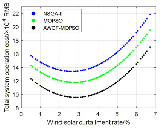
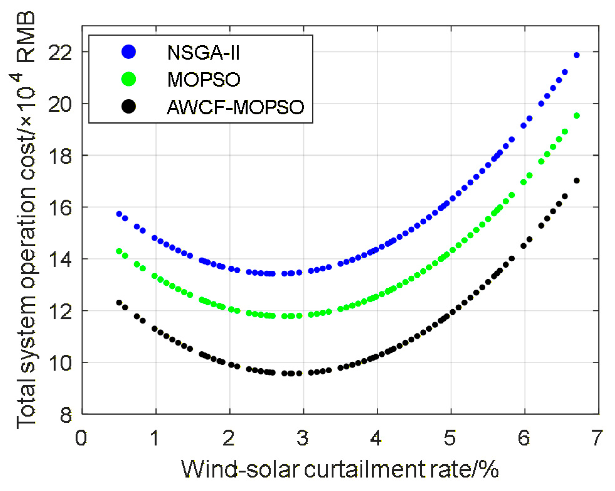
To clearly verify the superiority of the optimal scheduling algorithm proposed in this paper, the Pareto fronts of traditional NSGA-II, MOPSO, and AWCF-MOPSO on the plane of total operation cost and wind-solar curtailment rate are compared, as shown in Figure 5.
Figure 5.
Comparison of Pareto-Optimal Fronts for Different Algorithms.
All compared algorithms are implemented under the same population size, maximum number of iterations, and hardware/software environment, and each algorithm is executed independently 30 times to eliminate randomness. The Pareto front of the AWCF-MOPSO algorithm is generally lower than that of NSGA-II and the traditional MOPSO algorithm, indicating that under the conditions set in this study, AWCF-MOPSO can better balance multiple objectives and achieve optimal optimization results. For example, when all three algorithms achieve a wind-solar curtailment rate of 2.84%, the total system operation cost obtained by the AWCF-MOPSO algorithm is 95,723.57 RMB, while the total system operation costs obtained by the NSGA-II and MOPSO algorithms are 134,448.33 RMB and 117,877.67 RMB, respectively.
5. Conclusions
In this study, a PIES model is first constructed, with a wind-solar and EV coupling mechanism and an EV charging-discharging incentive mechanism designed to improve renewable energy utilization, reduce carbon emissions, and mitigate wind-photovoltaic curtailment. Subsequently, an improved MOPSO algorithm (AWCF-MOPSO) with adaptive weight comprehensive fitness is proposed, which realizes the collaborative optimization of PIES’ low-carbon, economic, and efficiency objectives by reconstructing the multi-objective function, designing a dynamic weight-adjustment mechanism, and optimizing inertia weight and particle-update strategy. Finally, three schemes are set up for simulation verification, and the main conclusions are as follows:
(1) Scheme 1 loses bidirectional flexible regulation capability, relying heavily on CHP units, gas turbines, and purchased energy to maintain power balance, resulting in high wind-solar curtailment, high energy purchase ratio, and the worst performance. Scheme 2 (unrestricted EV charging-discharging) reduces the curtailment rate to ~9% through peak discharging, but lacks deep coupling between EV scheduling and wind-solar characteristics, failing to maximize clean energy utilization and leaving room for optimization in economy and environmental protection.
(2) Scheme 3 achieves the optimal comprehensive performance. It realizes collaborative scheduling of EV charging for wind-solar absorption and discharging for peak compensation, reducing the wind-solar curtailment rate to less than 3%, ensuring real-time electric-thermal load balance, improving clean energy accommodation, reducing operation costs, and smoothing the load peak-valley difference through multi-equipment and multi-energy collaboration.
(3) Within the setting and conditions of this study, the proposed AWCF-MOPSO algorithm effectively addresses the deficiencies of conventional multi-objective optimization algorithms. Its Pareto front is consistently located below that of NSGA-II and traditional MOPSO, which means the proposed method can achieve higher renewable energy accommodation with lower system cost under the constraints of this paper, thereby offering reliable algorithmic support for the low-carbon optimal scheduling of park-integrated energy systems.
The above results indicate that this study promotes renewable energy accommodation by constructing a mathematical model of wind power, photovoltaic, and EV coupling, and introducing an incentive mechanism to guide users’ charging and discharging behaviors. By improving the fitness and convergence performance of the multi-objective particle swarm optimization algorithm, its performance in the low-carbon optimal scheduling of the PIES is enhanced, realizing the multi-objective collaborative optimization of carbon emission cost, total system operation cost, and wind-photovoltaic curtailment rate, which provides a theoretical reference and engineering practice basis for the low-carbon optimization of park integrated energy.
Author Contributions
Conceptualization, Y.Z. and J.W.; methodology, J.W.; software, J.W.; validation, J.W.; formal analysis, J.W.; investigation, J.W.; resources, Y.Z. and H.X.; data curation, J.W.; writing—original draft preparation, J.W.; writing—review and editing, Y.Z. and J.W.; visualization, J.W.; supervision, Y.Z. and H.X.; project administration, H.X.; funding acquisition, Y.Z. and H.X. All authors have read and agreed to the published version of the manuscript.
Funding
This study was supported by the Shanghai Natural Science Foundation, grant number: 23ZR1425000.
Data Availability Statement
The data presented in this study are available on request from the corresponding author. The data are not publicly available due to privacy restrictions.
Acknowledgments
The authors would like to express their sincere gratitude to all individuals and institutions that provided administrative and technical support during the research and manuscript preparation process. Special thanks are extended to the technical staff who offered assistance in experimental operations and data processing.
Conflicts of Interest
The authors declare no conflicts of interest.
Abbreviations
The following abbreviations are used in this manuscript:
| PIES | Park integrated energy system |
| IES | Integrated energy system |
| EV | Electric vehicle |
| V2G | Vehicle to grid |
| WP | Wind power |
| PV | Photovoltaic |
| NSGA-II | Non-dominated sorting genetic algorithm II |
| BWO | Beluga whale optimization |
| AWCF-MOPSO | Adaptive weight comprehensive fitness multi-objective particle swarm optimization |
| CHP | Combined heat and power |
| GT | Gas turbines |
| GB | Gas boilers |
| EB | Electrical boilers |
| EL | Electrolyzers |
| HFC | Hydrogen fuel cells |
| EES | Electrical energy storage |
| TES | Thermal energy storage |
| TOU | Time-of-use |
| MOP | Multi-objective optimization problem |
| MOPSO | Multi-objective particle swarm optimization |
Appendix A
Table A1.
Equipment parameters.
Table A2.
Other necessary parameters.
Figure A1.
Flowchart of the proposed AWCF-MOPSO algorithm.
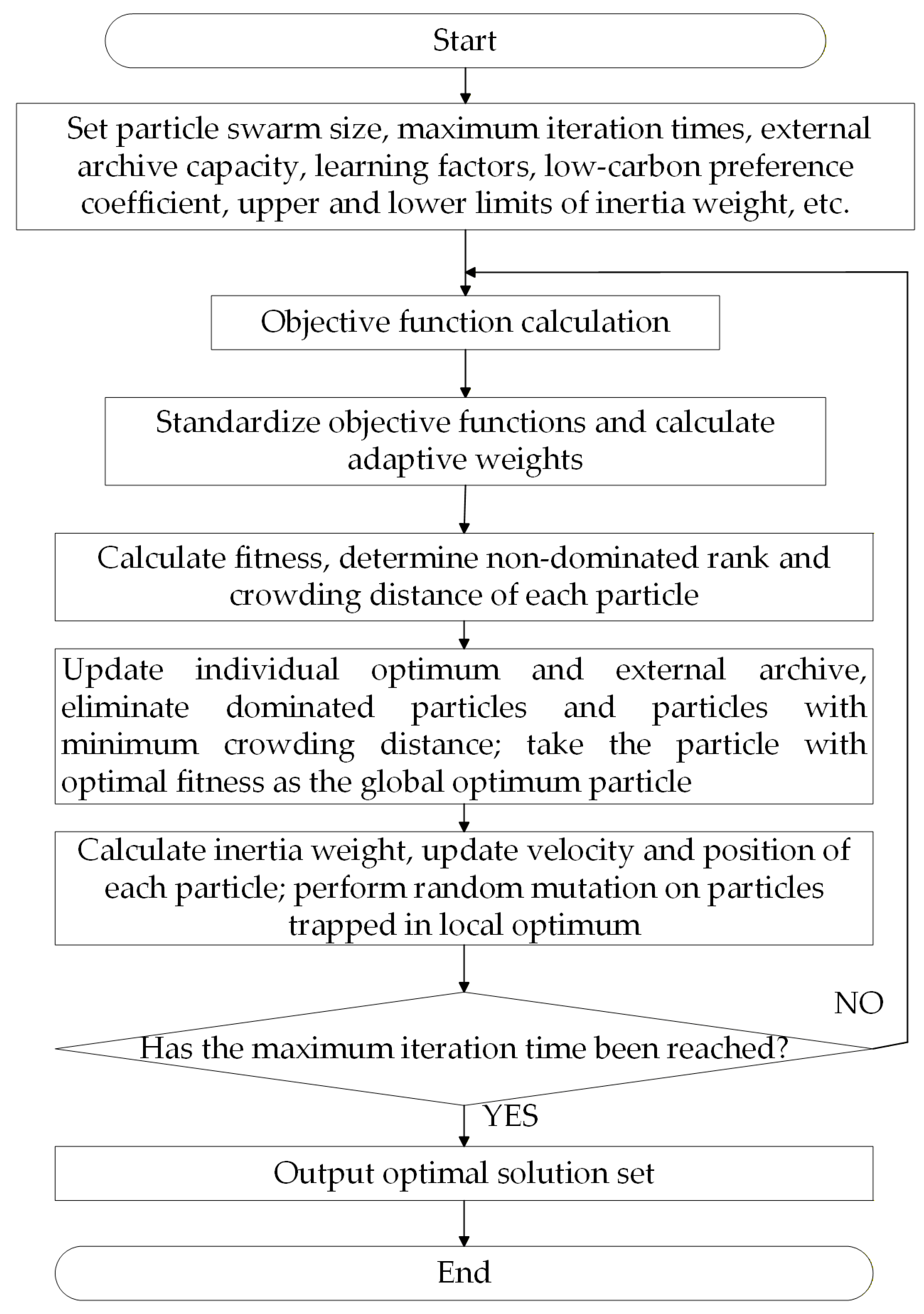
Figure A2.
Probability Distribution of EV Access and Departure.
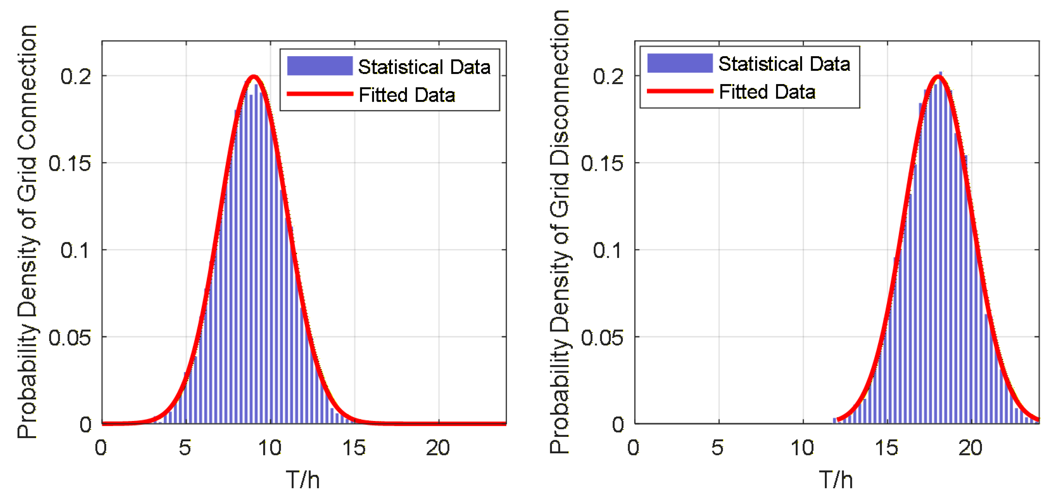
Figure A3.
(a) Grid Time-of-Use Electricity Price; (b) Wind and Photovoltaic Power Output.
References
- Lu, L.; Qin, Z. Low-carbon planning for park-level integrated energy system considering optimal construction time sequence and hydrogen energy facility. Energy Rep. 2023, 9, 554–566. [Google Scholar] [CrossRef] [Scilit]
- Zhang, Y.; Zhang, P.; Du, S.; Dong, H. Economic Optimal Scheduling of Integrated Energy System Considering Wind–Solar Uncertainty and Power to Gas and Carbon Capture and Storage. Energies 2024, 17, 2770. [Google Scholar] [CrossRef] [Scilit]
- Qiao, B.; Xu, H.; Liu, Y.; Ye, J.; Hu, H.; Yan, L.; Wei, T. Economic, Low-Carbon Dispatch of Seasonal Park Integrated Energy System Based on Adjustable Cooling–Heating–Power Ratio. Energies 2025, 18, 5071. [Google Scholar] [CrossRef] [Scilit]
- Hu, W.; Shen, H.; Ma, M.; Tian, Z.; Dong, Y.; Zhang, B.; Xie, W. An optimal scheduling method of integrated energy system in industrial parks considering carbon trading and electric vehicle charging load. Sci. Rep. 2025, 15, 40923. [Google Scholar] [CrossRef] [Scilit] [PubMed]
- Liu, Y.; Cao, X.; Zhang, Y. Park Integrated Energy System Optimization Considering Carbon Excess Ratio and Electric Vehicle Coupling. Energy Eng. 2025, 122, 3377–3398. [Google Scholar] [CrossRef] [Scilit]
- Liang, W.; Wang, S.; Li, X.; Li, X.; Xu, K. Optimization method of low carbon park integrated energy system based on multi-agent game. Electr. Power Syst. Res. 2025, 243, 111484. [Google Scholar] [CrossRef] [Scilit]
- Shao, X.; Huang, Y.; Duan, M.; Fang, K.; He, X. Optimal Dispatch for Electric-Heat-Gas Coupling Multi-Park Integrated Energy Systems via Nash Bargaining Game. Processes 2025, 13, 534. [Google Scholar] [CrossRef] [Scilit]
- He, C.; Xie, J. Two-stage operation optimization strategy of park integrated energy system cluster coupled with hydrogen energy storage. Energy Rep. 2025, 13, 1846–1858. [Google Scholar] [CrossRef] [Scilit]
- Zhao, Y.; Yang, Z.; Guo, Y.; Song, H.; Sun, H. An optimal dispatch strategy of off-grid park integrated energy system considering source volatility. Energy Rep. 2024, 12, 1597–1607. [Google Scholar] [CrossRef] [Scilit]
- Jia, X.; Yang, Y.; Du, J.; Gan, H. Research on robust optimization of the integrated energy system in industrial parks based on adaptive genetic algorithm. J. Phys. Conf. Ser. 2024, 2788, 012014. [Google Scholar] [CrossRef] [Scilit]
- Pu, Q.; Chen, X.; Shen, B.; Fu, L. Low-Carbon Economic Dispatch of Agricultural Park Integrated Energy Systems Based on Improved Multi-Objective Grey Wolf Optimizer. Energies 2025, 18, 6138. [Google Scholar] [CrossRef] [Scilit]
- Yu, X.; Song, Y.; Sun, R. Distributed cooperative electricity-carbon trading for multi-park integrated energy systems. Sustain. Energy Grids Netw. 2025, 43, 101683. [Google Scholar] [CrossRef] [Scilit]
- Wu, X.; Liao, B.; Su, Y.; Li, S. Multi-objective and multi-algorithm operation optimization of integrated energy system considering ground source energy and solar energy. Int. J. Electr. Power Energy Syst. 2023, 144, 108529. [Google Scholar] [CrossRef] [Scilit]
- Zhang, Y.; Zhao, H.; Li, B.; Wang, X. Research on dynamic pricing and operation optimization strategy of integrated energy system based on Stackelberg game. Int. J. Electr. Power Energy Syst. 2022, 143, 108446. [Google Scholar] [CrossRef] [Scilit]
- Luo, X.; Ranazzi, P. Better stopping through cross validation in an iterative ensemble smoother: A perspective from supervised machine learning. Geoenergy Sci. Eng. 2024, 243, 213298. [Google Scholar] [CrossRef] [Scilit]
- Wu, Y.; Wang, C.; Wang, Y. Cooperative game optimization scheduling of multi-region integrated energy system based on ADMM algorithm. Energy 2024, 302, 131728. [Google Scholar] [CrossRef] [Scilit]
- Zhao, Y.; Shi, L.; Chen, S.; Sun, B.; Zheng, Y.; Gao, J.; Xu, Z.; Wang, D.; An, Q. Scheduling optimization of IES based on improved particle swarm algorithm. J. Phys. Conf. Ser. 2023, 2655, 012015. [Google Scholar] [CrossRef] [Scilit]
- Sun, H.; Cui, Q.; Wen, J.; Kou, L. Optimization and scheduling scheme of park-integrated energy system based on multi-objective Beluga Whale Algorithm. Energy Rep. 2024, 11, 6186–6198. [Google Scholar] [CrossRef] [Scilit]

Disclaimer/Publisher’s Note: The statements, opinions and data contained in all publications are solely those of the individual author(s) and contributor(s) and not of MDPI and/or the editor(s). MDPI and/or the editor(s) disclaim responsibility for any injury to people or property resulting from any ideas, methods, instructions or products referred to in the content. |
© 2026 by the authors. Licensee MDPI, Basel, Switzerland. This article is an open access article distributed under the terms and conditions of the Creative Commons Attribution (CC BY) license.