


Abstract
Propylene hydroformylation is a typical large-scale gas–liquid reaction. Nevertheless, exorbitant costs and theoretical studies lagging far behind practical industry have prevented advancements in reactor efficiency. In this work, the flow, mass transfer, and reaction processes within the gas–liquid reactor were simulated using a three-dimensional CFD-PBM coupled model. The coupling processes between the flow field, mass transfer, and reaction in the gas–liquid reactor are clarified in this study. It provides precise direction for further process optimization by introducing the Hatta number as a quantitative criterion to determine the reaction’s controlling step (mass transfer-controlled or reaction-controlled). The constraints of conventional single-point analysis were overcome by visualizing a Ha number distribution contour, which showed that about 65% of the volume inside the propylene hydroformylation reactor is in a mass transfer-limited state. Based on this, operational parameter optimization was carried out, and the findings show that reaction efficiency may be successfully increased by reasonably raising the superficial gas velocity and system pressure within a certain range. The conversion rate increased by 23% when the superficial gas velocity doubled and by two times when the pressure doubled. Additionally, the effects of the stirring device and rotational speed were investigated, resulting in a 19% increase in conversion rate after optimization. The design and process optimization of similar hydroformylation gas–liquid reactors can benefit from this research.
1. Introduction
The process by which an alkene reacts with hydrogen and carbon monoxide under the influence of a catalyst to concurrently add a hydrogen atom and a formyl group to the alkene’s double bond is called hydroformylation. With 100% atomic economy, it can transform alkenes into higher-value aldehydes, which can be used as precursors to produce downstream chemicals with substantial economic value, such as amines, alcohols, and carboxylic acids [1]. Butyraldehyde is the main product of propylene hydroformylation. It is an essential feedstock for many fine chemical products and a crucial intermediate in the production of significant organic compounds, such as butanol and octanol.
Rhodium-based catalysts are frequently used in the hydroformylation of short-chain olefins because of their mild reaction conditions, great selectivity, activity that is 1000 times more than that of cobalt-based catalysts, and exceptional stability [2,3]. Homogeneous catalytic hydroxylation produces more than 10 million tons of aldehydes annually, accounting for approximately 75% of the worldwide supply of carbonyl synthesis products. Triphenylphosphine-modified rhodium catalysts remain one of the most popular catalysts for propylene hydroformylation [4].
Hydroformylation using rhodium–phosphorus complexes as catalysts is a typical gas–liquid reaction, while bubble column reactors are the most widely used reactor type for propylene hydroformylation [5]. Although bubble columns have benefits such as a straightforward structure and a good interfacial contact area, these reactors often have a high volume and dead zones in the flow, which prevent the catalyst from being fully utilized and lower the total reaction efficiency. Additionally, localized high temperatures caused by an uneven concentration distribution can affect reaction selectivity and perhaps deactivate the catalyst, leading to the loss of costly rhodium. A common industrial reactor for propylene gas–liquid reactions is the bubbling stirred tank, which basically consists of a bubbling tower with a mechanical stirring system. Mechanical stirring can efficiently increase mass transfer and decrease dead zone areas by introducing significant shear forces. However, theoretical research on these gas–liquid reactors lags far behind their industrial applications. Two constraints limit development and application at the laboratory stage: the perception that development costs are too high for certain small-scale applications, and the requirement to use highly poisonous carbon monoxide under pressure for hydroformylation. According to surveys, the number of academic articles addressing specific elements of hydrochlorination reactions has consistently increased over the past few decades, while the number of patents has remained below 100 annually [6].
The structure and operating conditions of gas–liquid reactors determine the transport characteristics and the chemical reactions occurring within the reactor. Thus, it is necessary to have models that can accurately describe the interaction phenomena across a broad range of parameters [7]. Unlike expensive traditional experiments, computational fluid dynamics (CFD) simulations have become an effective tool for researching the fluid dynamics of multiphase reactors at a low cost due to advancements in computational efficiency. The mass transfer, flow field and gas volume fraction within the reactor can all be precisely predicted by CFD [8].
Previous studies on bubble columns have mostly concentrated on high-precision measurement of flow dynamics inside the reactor or on reasonably well-established absorption mechanisms. Taborda et al. [9] used the LES–Euler–Lagrange approach to simulate bubble columns numerically. They discovered that using a full bubble dynamics model was the only way to achieve great data agreement by adding randomly generated eccentricities and motion angles to the bubble oscillation model. It was shown by Amaral et al. [10] that both mass transfer and bubble size are very dynamic in both space and time. Chen et al. [11] thoroughly examined the mass transfer behavior and gas–liquid fluid dynamics in a gas–liquid vortex reactor using a multiphase Euler–Euler CFD model combined with the Population Balance Model (PBM), mass transfer, and reaction models. He accurately simulated the reactive absorption of carbon dioxide in a monoethanolamine aqueous solution. Nevertheless, the majority of current research uses enhancement factors to depict the impacts of reactions, which is an empirical approach and lacks corresponding parametric support for specific reactions. Liu et al. [12] employed two enhancement factor models to simulate gas–liquid mass transfer behavior in a rectangular bubble column and compared the simulation results with published experimental data, finding significant discrepancies between the different models.
Meanwhile, there are not many studies on CFD models for particular reactions, like the hydroformylation process. Reactions, mass transport, and fluid dynamics all have intricate dynamic interactions. Studies on particular reactions are essential because industrial applications are the ultimate goal of reactor development. Despite doing experimental research on the hydroformylation reaction of 1-hexene, Zhao et al. [13] lacked a thorough understanding of flow and mass transfer behavior. Both the bubble diameter and mass transfer coefficient were treated as constants. Moreover, relatively well-established reaction processes, such as CO2, have been the main topic of the mass transfer. Darmana et al. [14] employed a three-dimensional discrete bubble model to investigate the intricate interactions involving fluid dynamics, mass transfer, and chemical reactions within a bubble column reactor. A surface renewal model was employed to calculate the mass transfer rate for an individual bubble. This model can predict bubble size distributions as well as the temporal and spatial variations in each chemical involved, but its study of the reactions is limited to systems with well-established parameters. Based on a two-fluid model, Ngu et al. [15] created a one-dimensional model of an industrial-scale biological methanation process. This model can forecast bioreactor performance and takes into consideration the fluid dynamics of bubble flow, multi-component mass transfer, and bioreaction kinetics. Nevertheless, complex fluid dynamic phenomena and concentration inhomogeneities present in real three-dimensional reactors cannot be well captured by the one-dimensional model. These findings show that CFD tools may be used to describe the intricate activity inside actual reactors, but more investigation is required to clarify the precise mechanisms and how they affect specific reactions.
Reactor performance can be enhanced through the use of agitation devices. To improve the practical value of our research, we plan to alter the internal structure of the previously mentioned model. Hydraulic and computational models have been extensively developed in recent decades to investigate mass transfer processes in agitated reactors [16]. The mass transfer rate of gas components in liquid within stirred two-phase flow reactors was predicted numerically by Varela et al. [17]. Experiments were used to determine the flow patterns and bubble behavior under various conditions, while numerical simulations were employed to obtain the flow field. However, bubble behavior was determined through experiments using air and water, whereas the simulations utilized the physical properties of the fluid from the actual reactor, thereby decoupling the interaction between flow and mass transfer. Breit et al. [18] coupled PBMs to describe the behavior of a dispersed gas phase in a thermostatic, non-reactive, gas–liquid, semi-batch stirred tank reactor. A new Gaussian-quadrature finite volume method was developed, demonstrating numerical robustness and accuracy across a wide parameter space. However, the model’s application is restricted because of its non-reactive character. Changes in the reactor configuration inevitably alter the flow conditions, which in turn affect mass transfer and reaction dynamics.
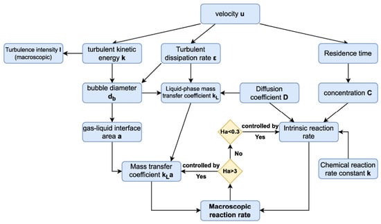
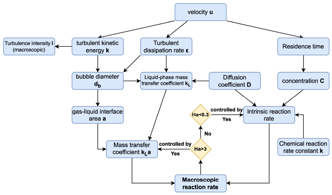
As shown in Figure 1, the flow, mass transfer, and reaction within the reactor constitute a complex system. Altering operating conditions, such as superficial gas velocity, results in different turbulent kinetic energies and dissipation rates, leads to changes in bubble size and mass transfer coefficients. Reactor performance is primarily reflected in the macroscopic kinetic rate, which is influenced by both mass transfer rates and intrinsic kinetic rates. The relationship between them can be bridged by the Hatta number, which includes the parameters of the intrinsic diffusion coefficient, the intrinsic mass transfer coefficient, and the intrinsic reaction rate constant. However, whether calculated at single points or averaged over volumes, the Hatta number obtained obscures significant variations within the reactor. Determining the Hatta number at a single point is unlikely to judge whether a reactor is driven by an intrinsic reaction rate or mass transfer rate. The reactor is a complicated interactive system, and data analysis and parameter acquisition are made possible via CFD. In addition, CFD tools enable the visualization of the Hatta number by providing contours.
Figure 1.
Schematic diagram of the coupling relationships among flow, mass transfer, and reaction.
So far, a thorough understanding of bubble columns’ characteristics has not yet been attained, due to the difficulty in adequately characterizing their intricate behavior and interactions. Additionally, with predictions of multiphase transport mostly relying on semi-empirical models or empirical correlations, establishing a logical connection between these factors remains a challenging task [19,20].
The work develops a CFD model that integrates flow, mass transfer, and reaction processes in the gas–liquid reaction to simulate the reactor parameters for propylene hydroformylation. The established model provides a technique for implementing and optimizing olefin hydroformylation processes, while also offering references for similar hydroformylation reactions.
2. Numerical Model
2.1. Governing Equations
A transient two-fluid Euler–Euler multiphase CFD model is employed to simulate gas–liquid interfacial flow, thereby replicating the real conditions within gas–liquid reactors. Since tracking a large number of bubbles requires significant computational time, the Euler–Euler method is commonly used for numerical simulations in bubbling columns. Furthermore, the high volume fraction of the dispersed phase makes the Lagrange method unsuitable for simulating turbulent mixing zones [21,22]. Therefore, the most popular technique for simulating bubble columns that operate at high gas volume fractions is the Euler–Euler method. According to the Euler model, every phase is uniformly distributed and continuous. In comparison to other multiphase flow models, it achieves a higher computational accuracy by using a set of equations that include several momentum equations and continuity equations for every phase in multiphase flow. The system of equations made up of continuity and momentum equations is used to solve each phase of a multiphase flow. The following formulas are used to determine mass and momentum conservation:
Mass conservation:
Momentum conservation:
where p, , , and denote the static pressure, stress tensor, density, and velocity vector, respectively. Phase q is indicated by the subscript q, where q = l and q = g represent the liquid and gas phases, respectively. represents gravity. Drag, lift, and other model-specific source terms are included in the external volumetric force .
2.2. Turbulence Model
Standard, RNG, and realizable k-ε turbulence models were compared by Laborde-Boutet et al. [23] to simulate bubble columns. The RNG model was found to be superior to the others due to its ability to accurately predict vortex flows and its applicability across a broader range of turbulence scales. Model-related equations are as follows.
Turbulent eddy viscosity equation:
k equation:
equation:
Bubble-induced turbulence:
where and respectively denote the turbulent kinetic energy generated by the mean velocity gradients and buoyancy forces in the gas and liquid phases. is the strain rate specific to RNG (which is zero in the standard and Realizable equation). and represent the source terms for bubble-induced turbulence. Fletcher et al. [24] found that accounting for bubble-induced turbulence generation is crucial for obtaining meaningful results. Neglecting this term leads to poor predictions of both the volume fraction and velocity. In the work, the model by Troshko and Hassan [25] is employed to simulate bubble-induced turbulence. The turbulence equations were divided into a single-phase term and an interface term. The single-phase term was modeled using the standard k-ε equation. Based on the assumption of low bubble inertia, a closure method for the interface turbulence term was proposed. It accounted for the additional pseudo-turbulence generated by bubble-induced mixing in the liquid phase. The validity of the established model was verified through liquid-phase velocity measurements. The modifiable constants used in the equations are listed in Table 1 [21].
Table 1.
Constants and values of RNG k-ε turbulence model.
2.3. Inter-Phase Force
Drag, added mass force, Basset force, lift, and wall lubrication force are examples of frequent interfacial forces. In studies by Laborde-Boutet et al., drag was the sole force examined, as it was deemed to differ by several orders of magnitude from other forces and play a crucial role in determining gas–liquid flow behavior [23,26].
2.3.1. Drag Force
Drag force results from the combined action of viscous and pressure differential on the bubble surface [27]. An empirical formula for drag force was proposed by Odar [28] in 1964, expressed as follows:
where is the drag coefficient, is the bubble diameter, is the liquid-phase density, and is the relative velocity between the gas and liquid phases.
The Tomiyama model is utilized for larger bubbles of different sizes, whereas the Schiller–Naumann resistance model is suitable for small bubbles. The Tomiyama model, which is ideal for gas–liquid flow with bubbles of various forms, is the drag model used in this work [29]. Here is the expression:
2.3.2. Swarm Factor
However, the previously indicated approach only works well for flows with modest gas volume fractions. There are often high gas volume fractions in the bubble column. Bubbles move through the bubble column in groups and form close clusters at high gas volume fractions. Within these bubble clusters, interactions between bubble boundary layers alter interphase momentum exchange and, most significantly, modify resistance. Because of the wake acceleration effect of large bubbles and the obstruction effect of small bubbles within bubble clusters, it is necessary to correlate the drag coefficient with the local gas volume fraction [30]. As stated by Varallo et al. [31], resistance models were unable to adequately represent hydrodynamics, resulting in a notable overestimation of the global gas volume fraction. To quantify this variance, the swarm factor h was developed by Gemello et al. [32] as the ratio of the actual resistance coefficient to the ideal resistance coefficient of the isolated bubbles.
Gemello et al. proposed a correlation by incorporating a minimum constant value . This approach produces computational fluid dynamics simulations that closely match experimental data while avoiding gas separation problems. It has only been validated for gas fractions below 30%. It is necessary to calibrate the adjustable parameter against experimental data. Superior results are obtained with = 0.15, corresponding to a sensitivity analysis of the values.
2.4. Population Balance Model
2.4.1. Bubble Size Distribution
Methods for simulating bubble size have a big impact on simulation outcomes. Different bubble sizes result in varying complexities of gas–liquid flow due to bubble shape and wake effects. Additionally, the interfacial area for gas–liquid mass transfer is strongly impacted by bubble size. Constant Bubble Size Modeling (CBSM) and Variable Bubble Size Modeling (VBSM) are the two types of bubble size modeling approaches. Khalil et al. [33] simulated a bubbling bed reactor under homogeneous conditions, demonstrating the importance of considering bubble size distribution for accurate mass transfer modeling. VBSM considerably resembled the actual processes.
The PBM is a conservation equation capable of tracking the dynamic evolution of particle properties. Wang et al. [34] demonstrated that the CFD-PBM coupled model is an effective method for predicting fluid dynamics, bubble size distribution, interfacial area, and gas–liquid mass transfer rates within bubble columns. Guo et al. [35] experimentally verified that the coupled model can quantitatively describe the influence of liquid properties on bubble size, interfacial forces, turbulence parameters, and bubble breakup and coalescence behavior.
Solving the group-balance equation is difficult because it is a continuous nonlinear partial differential equation. The continuous bubble size distribution is discretized into bins of varying sizes using the discrete VBSM method. According to Gaurav et al. [21], models with more bubble phases produced superior results in agitated-turbulent regions. The following geometric sequence is used to determine the bubble diameter interval linked to each bin:
where is the bubble volume in the i-th tank. In relation to bubble diameter:
We set the number of boxes to 12, as it has been demonstrated to represent a favorable compromise between accuracy and computational time. With q set to 1.4 and a minimum diameter of 1 mm selected, the maximum permissible bubble size is 35 mm.
2.4.2. Breakup Model
Breakup mechanisms can be categorized into four main types: turbulent fluctuations, macroscopic shear stress, shear processes, and interfacial slip instabilities. In turbulent gas–liquid systems, the first group of mechanisms is paramount, as bubble breakup in industrial equipment is primarily driven by turbulent pressure fluctuations at surfaces and collisions between bubbles and vortices. The kinetic theory of droplet and bubble breakup in turbulence provided the foundation for the bubble breakup model proposed by Luo and Svendsen [36]. They contended that bubbles only burst when the kinetic energy of turbulent vortices surpasses the rise in surface energy needed for breakup.
2.4.3. Coalescence Model
Compared to breakup, bubble coalescence is more intricate. In addition to interactions between bubbles and the continuous phase, this phenomenon also includes interactions with nearby bubbles after collisions due to forces and flow. Turbulent vortices within the reactor not only transport bubbles but also interact with them, ultimately leading to collisions. When two bubbles collide, coalescence occurs if the contact time exceeds that required for the liquid film between them to drain to the critical breakup thickness. Therefore, the ratio of contact time to coalescence time serves as the primary indicator for determining whether coalescence will occur. Luo’s bubble coalescence model is used in this work:
Simulation results indicate that as liquid viscosity increases, the probability of bubble coalescence between two bubbles rises, leading to the formation of large bubbles and promoting bubble coalescence. Increased liquid viscosity enhances the stability of large bubbles and requires greater energy for their rupture into smaller bubbles. The bubble coalescence coefficient influences simulation outcomes. To account for variations in liquid viscosity, we referenced the literature employing solvents with comparable viscosities and set the coalescence coefficient to 0.9 [37].
2.5. Reaction Process
Propylene hydroformylation is a common gas–liquid process that is mostly utilized to produce butyraldehyde [38] (Figure 2). Propylene is in the liquid phase of this process, whilst H2 and CO are in the gas phase. Fluid dynamics, mass transfer, and chemical reactions, along with their effects, are entirely transient and highly interrelated. Therefore, in such simulations, every feature should be taken into account. Simulation results using different mass transfer rate models exhibit significant differences, making this a primary factor affecting the accurate prediction of chemical reaction processes.
Figure 2.
Equation for propene hydroformylation reaction.
To verify the reasonableness of the model settings in this simulation, the simulation parameters in this research are compared to the experimental and simulation parameters of Bernas et al. [38,39]. The reaction was conducted in a semi-batch reactor using Rh as the catalyst precursor and cyclohexyl diphenylphosphine as the ligand.
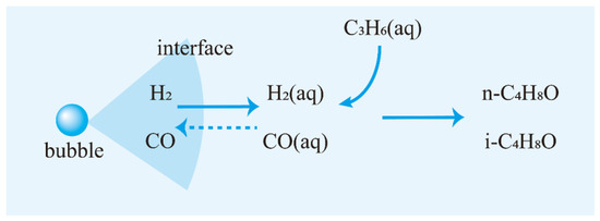
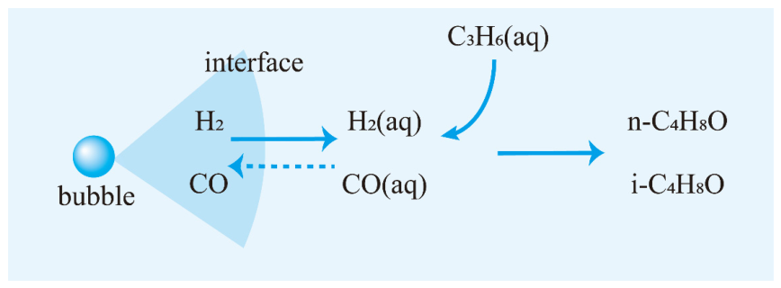
The mass transfer and reaction processes occurring at the internal gas–liquid interface are shown in Figure 3. It can be broken down into two sequential steps: first, gaseous CO and H2 diffuse into the liquid phase through the interface. And then CO and H2 react with the propylene pre-dissolved in the solvent to produce n-butyraldehyde as the primary product and iso-butyraldehyde as the by-product. Furthermore, when establishing the computational fluid dynamics model for propylene hydroformylation, mass transfer and reactions are simplified:
Figure 3.
Mass transfer and reaction processes at the gas–liquid interface.
- 1.
- The flow and mixing of reaction materials take place within the reactor, with negligible changes in the catalyst and ligands within the solvent.
- 2.
- Gaseous materials undergo unidirectional mass transfer to the liquid phase in the reactor.
- 3.
- Only in the liquid phase does the reaction occur.
Previous studies have employed similar simplifications. Fletcher et al. [24] assumed no resistance on the gas side and modeled O2 transport from gas to liquid using diffusion-limited mass transfer. For the product butyraldehyde, experimental data indicate that only a small amount is generated within the relatively short simulation timeframe, with most dissolving into the liquid phase. Its partial pressure in the gas phase is negligible, allowing its gas-phase concentration to be disregarded. Therefore, the reverse transport process for the product is omitted.
The component transport equation is as follows:
where Ri is the net production rate of homogeneous species i generated by chemical reactions, and Si is the production rate from dispersed phase additions and user-defined source terms. In turbulent flow, mass diffusion can be expressed as:
where Sct, μt, and Di represent the turbulent Schmidt number, turbulent viscosity, and diffusion coefficient for species i, respectively.
Mass transfer of gaseous substances occurs at the interface between bubbles and the liquid bulk phase. The substantial impact of mass transfer resistance was shown experimentally and numerically by Bernas et al. [38], who also proposed an interfacial mass model for multiphase chemical processes at the bubble–liquid interface. In this model, the chemical composition of small bubbles is assumed to consist of CO and H2. Due to the low solubility of CO and H2 in the experimental solvent, mass transfer resistance is concentrated in the liquid film:
where kLa represents the mass transfer parameter, kL is the liquid-phase mass transfer coefficient, and a is the gas–liquid interface area. Concentration changes are divided into two main components: reaction source terms and mass transfer source terms. The reaction source term calculates the consumption of reactants and the production of products during the hydroformylation. The mass transfer source term calculates mass transfer at the microbubble–liquid interface, expressed using a double-film model combined with Henry’s law.
For the mass transfer source term, it is rewritten in the form expressed by Zhao et al. [13] using Henry’s constant:
In the equation, represents the Henry’s law constant expressed in terms of concentration and is dimensionless. The literature indicates that the solubility relationship follows the following equation [40]:
The values for A, B, and C of H2 and CO are 10.972, −1466.01, and −2.393 L, and 17.413, −1398.4, and −3.419, respectively. The Henry’s constants for CO and H2 under the current operating conditions were calculated to be 4.40 and 7.58, respectively.
In the literature, similar values for kLa in stirred tank reactors have been reported to range from 0.05 to 0.2 s−1.
is the gas-phase gas volume fraction, is the Sauter diameter of the bubble, Sh is the Sherwood number calculated using parameters provided by Bird [36], D is the diffusion coefficient, and D is calculated using the expression provided by Wilke–Chang [41].
where Re denotes the Reynolds number, Sc represents the Schmidt number, is the slip velocity, is the association parameter (taken as 1.4), and VA is the molar volume of the gas. The VA values for CO and H2 are 30.7 cm3/mol and 14.3 cm3/mol, respectively.
For the reaction source term, the work describes the hydroformylation of propylene as two catalytic pathways yielding n-butyraldehyde and i-butyraldehyde, neglecting the effects of other side reactions. The reaction equations are as follows:
The main reaction:
The side reaction:
rN and rI stand for the production rates of the reaction products n-butyraldehyde and i-butyraldehyde, respectively. The simplified expression of the reaction rate was given by Bernas et al. [38]:
In the equation, (kmol/m3), (kmol/m3), (kmol/m3), (mass fraction), and (mass fraction) denote the concentrations of propylene, hydrogen, and carbon monoxide, the mass fraction of the metal (rhodium), and the mass fraction of the ligand, respectively. indicates that the reaction rate is independent of the mass fraction of rhodium. The constants a and b are independent of temperature. The relevant parameters in the equation are shown in Table 2.
Table 2.
Estimated parameter values.
Both the source terms for reaction and mass transfer are input into the reactor’s full fluid domain via our custom code, acting on each cell within the fluid domain.
The actual process within a reactor is a complex system. The reaction rate is not determined solely by the intrinsic chemical reaction kinetics but is also significantly constrained by mass transfer efficiency. The Hatta number is an extremely important dimensionless number in gas–liquid reaction engineering, defined as the ratio of the maximum possible intrinsic chemical reaction rate to the maximum possible mass transfer rate.
Ha established a quantitative relationship between flow patterns, mass transfer, and reactions, which serves as the theoretical foundation for understanding and optimizing gas–liquid reactors. It is used to quickly identify the rate-limiting step in a gas–liquid reaction. When Ha > 3, the reaction is fast. The liquid film is where most reactions take place. Before entering the bulk liquid phase, gas-phase reactants are almost completely exhausted. The process is mass transfer-controlled, and the mass transfer rate determines the overall reaction rate. The reaction is delayed when Ha is less than 0.3. The bulk liquid phase is where most reactions take place. At this stage, intrinsic reaction kinetics govern the process.
2.6. Simulation Settings
Simulations were performed using commercial software STAR CCM+ 19.02. A pressure-based finite volume method is employed to solve the discretized equation system. Selected numerical models and parameters used in this work, including solution techniques and boundary conditions, are shown in Table 3.
Table 3.
Model settings used in this work.
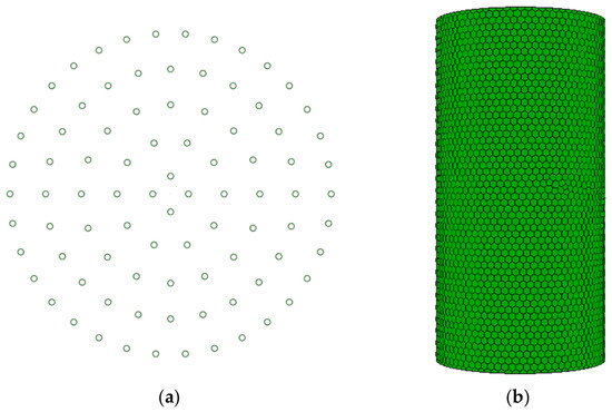
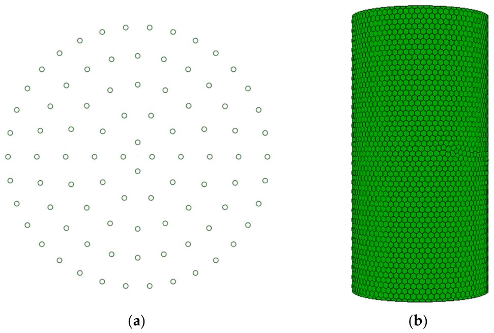
The gas–liquid reactor in this paper is based on Bernas’ case study. Since two-dimensional tools cannot accurately model the structure of the sparger, we created a three-dimensional reactor model. The reactor is cylindrical, which has a diameter of 0.5 m and a height of 1 m. As shown in Figure 4a, the gas inlet is a gas distributor located at the center of the bottom. The gas is injected into the tower from the bottom through the distributor. The sparger structure consists of 88 small holes with a diameter of 5 mm, arranged as illustrated. The inlet is defined as a velocity inlet, with the corresponding inlet gas velocity calculated using the superficial gas velocity. The feed composition consists of equimolar CO and H2, each accounting for a 50% molar fraction of the gas. For the gas inlet, the inlet gas volume fraction is set to 1. The bubble size distribution is narrow, and based on literature studies, the inlet bubble velocity should be close to 3–4 mm. Therefore, Bin-7 is selected as our inlet bubble size. A no-slip boundary condition is applied to the walls. A pressure outlet boundary condition is specified at the top of the tower, with the outlet located at the top center and subjected to complete gas reflux. The operating pressure is set to 1 MPa, and the temperature is 373 K. Since this is a semi-batch reactor, there is no liquid inlet or outlet.
Figure 4.
Model structure and mesh. (a) Sparger structure; (b) model mesh.
The solvent within the reactor is 2,2,4-trimethyl-1,3-pentanediol monoisobutyrate, with propylene pre-dissolved in the liquid phase. The initial static liquid level height was set to 0.5 times the total reactor height for comparison with experimental cases to validate model rationality. Subsequent operations and process parameter studies set the static liquid level height to 0.65 times the total reactor height to better align with industrial practice.
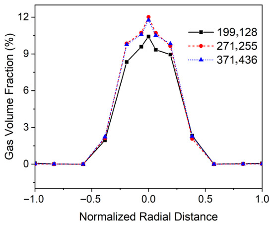
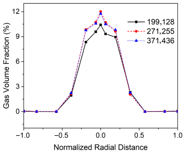
Figure 4b shows the model’s mesh. The minimum mesh size was set to 1 mm and the number of mesh elements to 271,255. The minimum orthogonal mass is 0.402, indicating that the mesh quality is good. As shown in Figure 5, the model underwent grid independence testing across three grid configurations (199,128, 271,255, 371,436). The model was set up as an air–water system under no mass transfer and reaction conditions, with a 60 s transient simulation run. Settings for the turbulence model, PBM and others remained consistent. The radial gas volume fraction at a height of 0.3 times the total reactor height was used as the evaluation metric. Figure 5 displays the radial gas volume fraction across different mesh resolutions. It is evident that the data from the 199,128-cell mesh significantly deviates from the high-resolution mesh, whereas the 271,255-cell mesh already achieves substantial agreement with the high-resolution quality. Therefore, this mesh resolution will be adopted for subsequent studies.
Figure 5.
Grid independence verification.
Transient simulations, lasting over 200 s, are initially validated against experimental data to confirm model validity. This duration represents a compromise between simulation validity and computational effort.
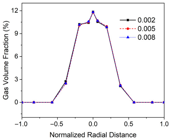
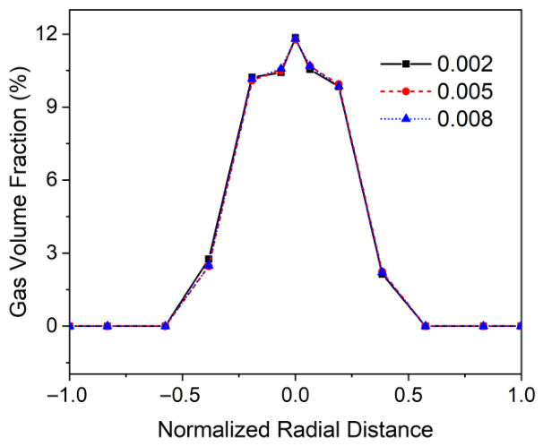
Varallo et al. [31] studied the fluid dynamics of large bubble columns operating over a wide range of superficial gas velocities. They discovered that the time step should be selected so that the Courant–Friedrichs–Lewy (CFL) ratio is less than 1, with an ideal value of Δt = 0.005 s. Sensitivity analysis was used to confirm that the time step was appropriate. The initial time step employed in our study was 0.001 s. The Courant number could be raised because an implicit technique was used and satisfactory convergence was seen. A time step of 0.005 s was used after 1 s of simulation, and stable results and good convergence were observed. A sensitivity analysis was carried out to investigate the independence of the numerical solution from the time step size, further confirming the rationale of the time step selection. By varying the time step size (Δt = 0.005 s) by 60%, two distinct time step sizes were evaluated. A 60 s transient simulation was performed using the full model under different time steps. The radial gas volume fraction distribution at 0.3 times the total reactor height for various time steps is depicted in the image (Figure 6). The results for different time steps are similar, indicating that the error introduced by the time step size in the solution is acceptable.
Figure 6.
Sensitivity analysis on the time step.
3. Results and Discussion
3.1. Model Validation
The model is validated based on the previous discussion, and parameters are adjusted using simulation and experimental data from Bernas [38]. The reaction rate was calculated using their kinetic equation. A comparison of the model with the experimental setup is shown in Table 4.
Table 4.
Model and experimental parameters.
For the validation model, a 20 min timeframe is chosen as it is long enough to exhibit the extent of reaction progress, and both mass transfer and reaction rates achieved comparatively steady values during this time. The data from Group A were chosen for comparison with the simulation because the simulation produced a volume-average kLa value of 0.019 s−1 for the model, which is close to the experimental values in Group A. The reaction conversion rates were employed for validation because the experiment only yielded concentration data.
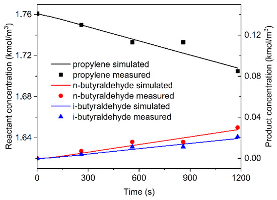
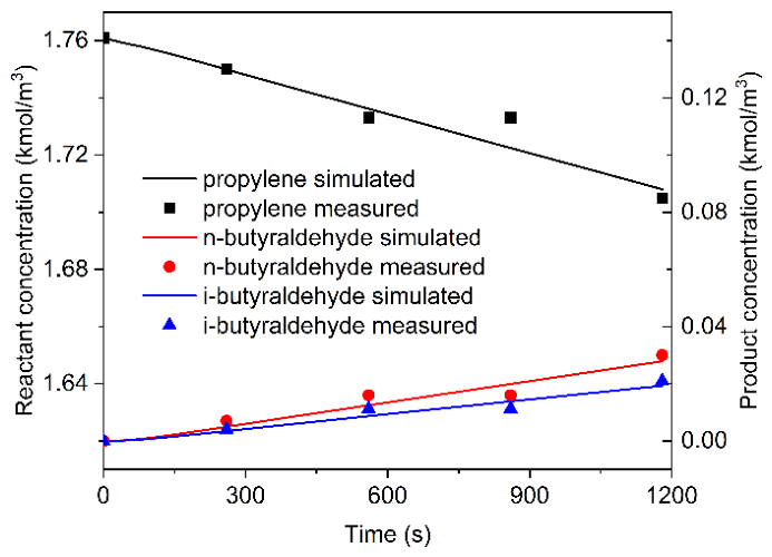
Figure 7 shows the concentration changes (kmol/m3) of propylene and the products in the liquid phase during a 20 min transient simulation. The black solid line represents propylene concentration, while the red and blue solid lines represent n-butyraldehyde and i-butyraldehyde concentrations, respectively. The concentration values are volume-integrated averages of the fluid region below 0.6 reactor height. Concentrations, mass transfer rates, and reaction rates in subsequent work are obtained using the same method.
Figure 7.
Comparison of simulation and experimental data.
During the transient simulation, the concentration of the reactant propylene gradually decreases over time, while the concentrations of the products butyraldehyde and iso-butyraldehyde gradually increase. The rate of reaction increases steadily throughout the first reaction phase. This acceleration is caused by several factors, including insufficient mass transfer of CO and H2 at the onset. After approximately 5 min, the concentration curve becomes relatively smooth and largely linear, reflecting the relatively constant rates of reactant consumption and product formation. The points in the figure corresponding to the colors of the curves represent the concentrations of reactants and products measured in the experiment. Overall, the simulated curves show good agreement with the experimental measurements.
As shown in Table 5, the conversion rates of propylene at four time points were calculated based on experimental and simulated data. As can be seen in Figure 6, the data point at 860 s deviates significantly from the overall trend and does not align with the theoretical values; this may be due to measurement errors. The maximum error for the remaining data points is 10.69%, and the average error is less than 10%, which is acceptable within the accuracy requirements for engineering analysis in this study. This indicates that the model configuration is reasonable, consistent with experimental data and physical principles, and holds practical significance for further research.
Table 5.
Data on conversions and errors.
3.2. Flow, Mass Transfer, and Reaction Structures
The focus of this study shifted to using the current computational fluid dynamics model to investigate the fundamental mechanisms of the intricate coupling between flow, mass transfer, and reaction within the propylene hydroformylation reactor after the model validation was finished. It was established that the model could accurately capture the macroscopic flow field and reaction patterns within the reactor.
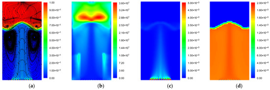
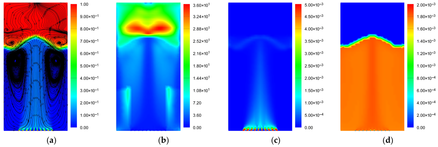
To analyze the mutual influence between flow, mass transfer, and reaction, we output the gas volume fraction and streamline diagrams (Figure 8a) for the z = 0 cross-section of the reactor (all axial sections later are also taken at the z = 0 plane), the Ha value of H2 with relatively lower solubility (Figure 8b), the H2 mass transfer rate (Figure 8c), and the formation rate of n-butyraldehyde (Figure 8d). The CO/H2 synthesis gas entering from the gas inlet rises as bubbles, as seen in Figure 8. The middle portion has a larger gas volume fraction, which progressively drops with height. This occurs as a result of bubbles accelerating and coalescing during ascent, which reduces the number of bubbles per volume. Steamtraces show that liquid is entrained upward as gas rises in the central region. A looping flow pattern is then created as the liquid descends again near the wall.
Figure 8.
Parameters inside the reactor. (a) Gas volume fraction and steamtraces; (b) Ha value; (c) mass transfer rate of H2 (kg/m3·s); (d) reaction rate of n-butyraldehyde (kg/m3·s).
The reactor’s actual operation is a complicated system. Simulation results indicate that the reaction rate is not solely determined by intrinsic chemical reaction kinetics but is significantly constrained by mass transfer efficiency. The Hatta number is used to quickly figure out what a gas–liquid reaction is controlled by. Traditional experimental methods cannot obtain Ha values for specific regions, whereas our work utilizes CFD tools to enable the visualization of Ha.
As shown in Figure 8b, low-Hatta-number regions appear near the bottom sparger and the axial center of the reactor. Turbulence intensity is highest at the gas inlet, where newly formed bubbles are small, interfacial renewal rates are extremely rapid, and mass transfer rates are high. The Ha value gradually increases with height, reflecting a decrease in mass transfer rates. This occurs because as bubbles rise, turbulent energy dissipates and mass transfer resistance increases. Furthermore, as Ha values in most other reactor regions are greater than 3, 65% of the area is limited by mass transfer. The rate at which H2 undergoes chemical reactions at the catalyst’s active sites is substantially faster than the one transported from the gas-phase bulk to those sites. Before the gaseous reactants penetrate the liquid-phase bulk, they are mostly consumed inside the liquid film close to the gas–liquid interface. Increasing gas–liquid mass transfer is currently the best way to improve reaction efficiency, which guides subsequent optimization research on operational and design parameters. This finding is further supported by contours of reaction and mass transfer rates. High reaction rates are often found in areas with high mass transfer rates.
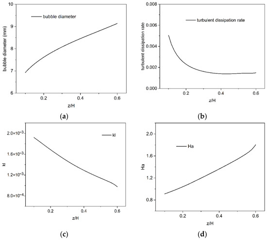
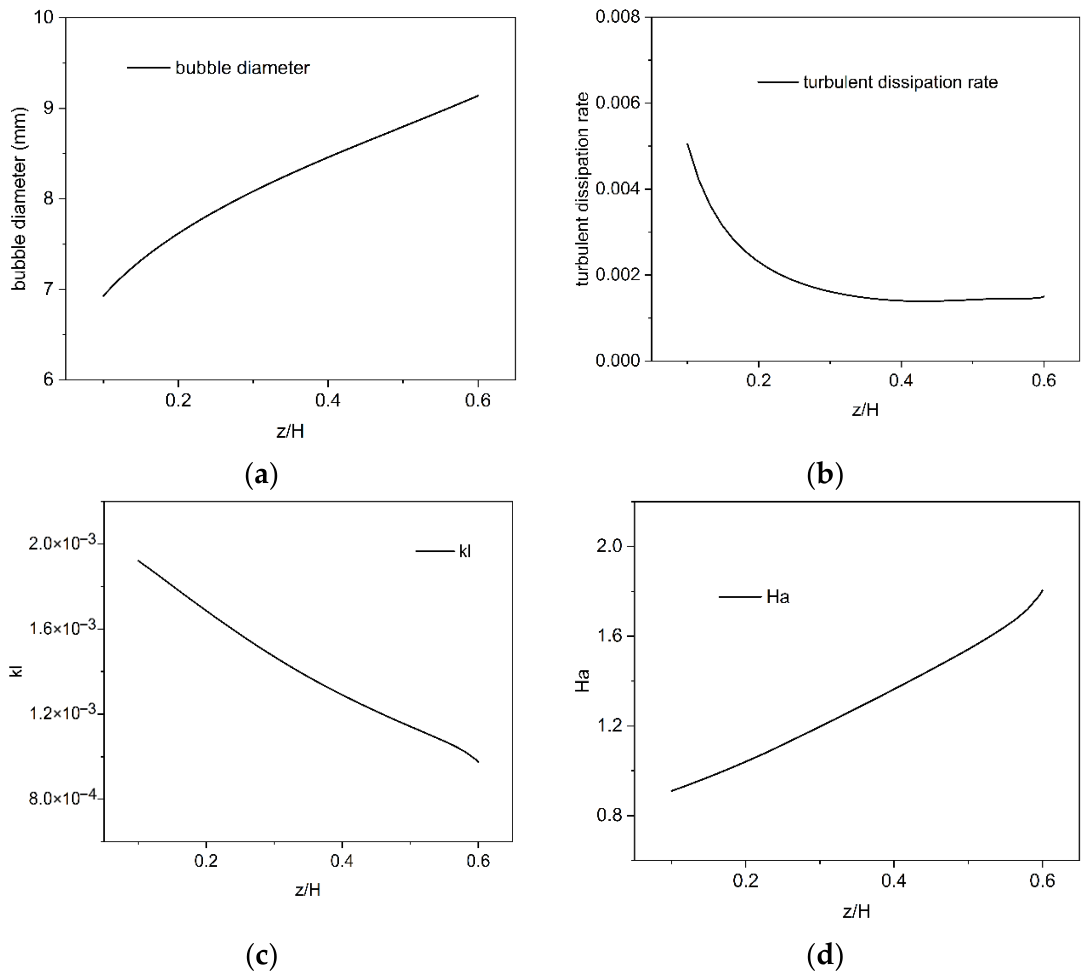
To better understand the intrinsic relationship between flow, mass transfer, and reaction, we analyzed parameters including the bubble size db, turbulent dissipation rate, liquid-phase mass transfer coefficient kL, and Ha value. We derived data for corresponding parameters at axial heights ranging from 0.1 to 0.6 times the total reactor height (Figure 9).
Figure 9.
Reactor parameters at z/H from 0.1 to 0.6. (a) Bubble diameter db (mm); (b) turbulent dissipation rate (m2/s3); (c) the value of kL (m/s); (d) the value of Ha.
As shown in Figure 9a, the bubble diameter continuously increases in the axial direction, primarily due to the coalescence behavior of bubbles. The bubble diameter may increase as a result of smaller bubbles merging with larger ones during ascent. Near the gas sparger, the fluid undergoes intense turbulence with higher turbulent kinetic energy and turbulent dissipation rate. As height increases, the turbulent kinetic energy gradually dissipates. Concurrently, the horizontal flow direction creates intricate eddy and vortex formations nearer the liquid surface, improving shear and turbulent dissipation.
According to a microscopic analysis of mass transfer processes at the bubble surface, the liquid-phase mass transfer coefficient kL is mainly a function of Sh and db, with db being the primary influence. kL decreases as db increases. From a macroscopic perspective, kL is proportional to the 1/4 power of the turbulent dissipation rate. Although the simulated data exhibit some deviation, they follow a similar trend. Ha, in turn, is inversely proportional to kL. As height increases, turbulent kinetic energy decreases, weakening mass transfer. Due to the relatively high gas volume fraction in the central axial region, Ha ranges approximately between 0.8 and 2. At this point, the macroscopic reaction rate is influenced by both the mass transfer rate and the reaction rate. Figure 9 reflects these observations.
Therefore, subsequent research will no longer be confined to merely observing changes in the ultimate conversion rate. Rather, by utilizing the existing model, we will methodically dissect how important variables, like pressure and superficial gas velocity, affect the reactor’s overall effectiveness. This will be accomplished by investigating the effects of these factors on the interfacial mass transfer, bubble behavior and flow field. Consequently, this approach will provide precise and in-depth theoretical guidance for achieving process optimization.
We can optimize reactor parameters using the information mentioned previously. Any modification to the reactor’s structure or operating circumstances will first disrupt the fluid dynamics inside the reactor, which will then cause variations in mass transfer and reaction rates, and ultimately show up as variations in reaction efficiency.
3.3. Influence of Operating Parameters
The propylene hydroformylation reaction is a typical process where gas-phase reactants dissolve into the liquid phase before reacting. In addition to the intrinsic chemical reaction rate, the mass transfer rate of the gas into the liquid has a significant impact on the reaction rate. Many variables, notably superficial gas velocity, pressure, temperature, feed composition, and reactor dimensions, affect mass transfer and reaction rates [42]. This section illustrates the impact of operating parameters on relevant reactor variables using superficial gas velocity and pressure as examples. Simulations are conducted over a 200 s timeframe, balancing computational accuracy and efficiency. Similar simulation durations are used in the majority of transient investigations of gas–liquid multiphase fluxes. Subsequent simulations in this work also showed that the reactor’s reactant and product concentration variations had mostly stabilized into a linear trend by 200 s.
3.3.1. Superficial Gas Velocity
Gas velocity is a critical parameter in reactor design, as it alters the flow patterns, gas volume fraction, bubble behavior and interfacial contact. The reaction rate is indirectly impacted by these variables. Actually, the velocity distribution at the gas sparger is influenced by several variables, including the pressure drop and the number of holes [43]. Nevertheless, this analysis’s computational complexity is outside the scope of this investigation. Therefore, for simplification, this work assumes that the gas inlet possesses a uniform velocity distribution. In the model settings, only the inlet gas velocity was altered, with values calculated from the corresponding superficial gas velocities: 0.568 m/s, 1.136 m/s, and 2.272 m/s. The gas volume fraction, feed composition, and initial bubble size were maintained at their original settings.
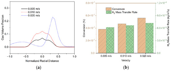
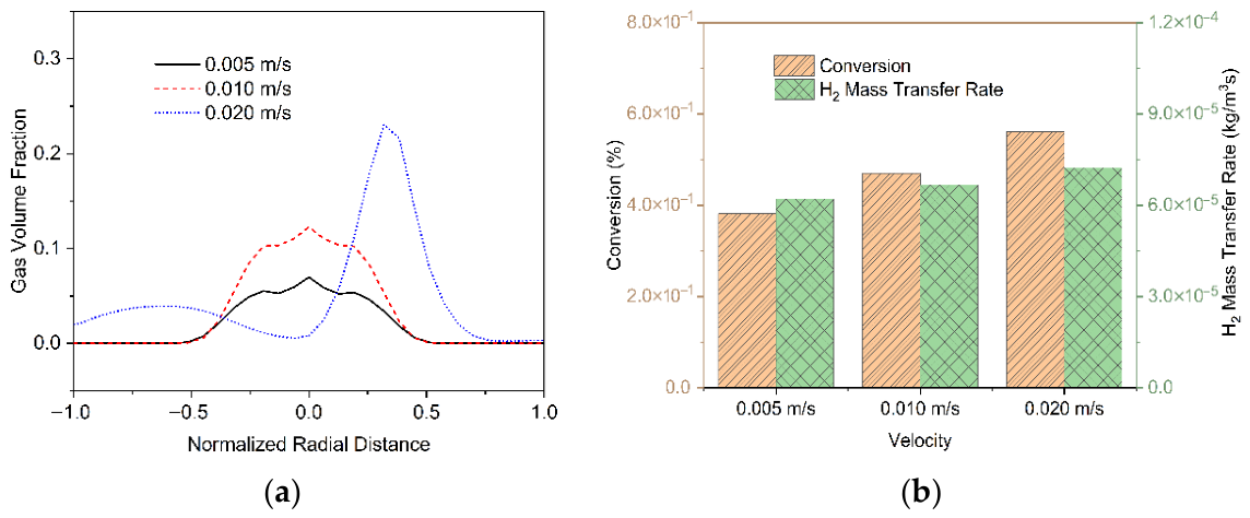
Figure 10 shows the radial gas volume fraction distribution, conversion rate, and H2 mass transfer rate at z/H = 0.3 within the reactor under different superficial gas velocities. As the velocity increases, the reactor’s axial gas volume fraction rises noticeably, as seen in Figure 10. Since more gas is injected per time at higher gas velocities, there are more bubbles trapped inside the reactor, thus increasing the gas volume fraction. The interface area a is proportional to the gas volume fraction, thereby also increasing. Greater turbulence is produced at high gas velocities because the gas’s quick ascent puts more agitation and shear forces on the liquid. This increases the mass transfer coefficient of the liquid phase kL. Since the overall mass transfer coefficient is proportional to the product of a and kL, the simultaneous enhancement of both significantly accelerates the dissolution of gaseous reactants. The dissolution of reactants leads to an increase in concentration, which accelerates the reaction rate. This improves the reactor’s space–time yield and propylene conversion. As shown in Figure 9b, when the superficial gas velocity increases from 0.005 m/s to 0.01 m/s, the conversion rate increases by 23%. Higher gas velocities also increase liquid circulation, which helps the reactor’s concentration and temperature distribution become more consistent.
Figure 10.
Partial parameters inside the reactor at 200 s under different velocities. (a) Gas volume fraction at z/H = 0.3; (b) conversion rate and H2 mass transfer rate.
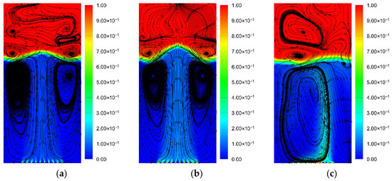
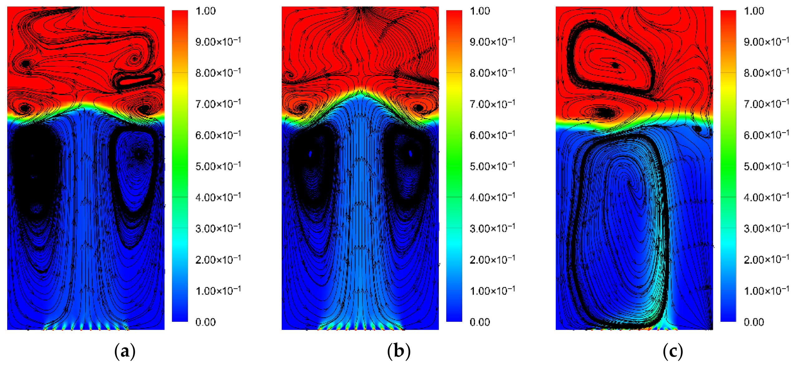
However, it should be noted that when the superficial gas velocity increases to 0.02 m/s, Figure 10a clearly shows a change in the flow pattern within the reactor, with the maximum gas volume fraction no longer occurring in the central region. We generated gas volume fraction and streamline contour plots at different velocities (Figure 11) to conduct an in-depth analysis of the flow conditions.
Figure 11.
Gas volume fraction and streamlines at different superficial gas velocities. (a) 0.005 m/s; (b) 0.01 m/s; (c) 0.02 m/s.
At low superficial gas velocities (0.005–0.01 m/s), the bubble ascent streamline is vertical, with a stable and symmetrical flow pattern forming two symmetrical liquid circulation zones. When the velocity increases to 0.02 m/s, gas deflection to the right and the peak of volume fraction deviation from the center occur. This generates an asymmetric pressure gradient. Liquid on the right side is entrained upward by the bubbles, shortening gas residence time. On the left side, liquid sinks due to insufficient buoyancy, forming a single large-scale circulation. Partial fluid flow within the reactor enters a short-circuited state, exacerbating concentration and temperature non-uniformity. Although conversion rates do increase at high gas velocities, this does not imply that increasing gas velocity is always advantageous. A significant portion of the turbulent kinetic energy generated by high flow rates is wasted. A rational assessment of the benefits and drawbacks of increasing gas velocity is essential.
Therefore, within a certain range of superficial gas velocities, increasing the gas velocity benefits the reaction system, and appropriately raising the gas velocity is an effective optimization strategy. However, attention must also be paid to changes in flow patterns at high gas velocities, and gas velocity should not be increased indiscriminately.
3.3.2. Pressure
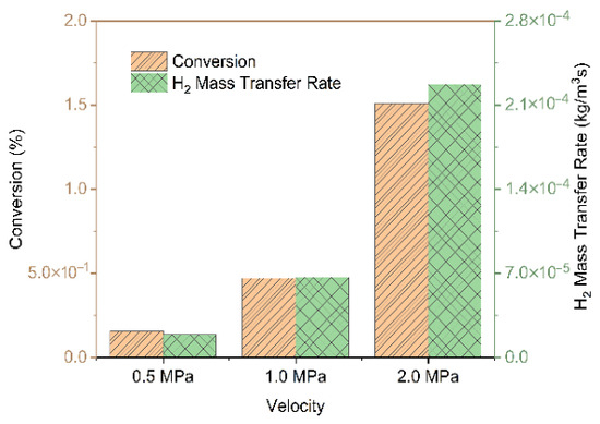
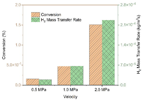
Reactant solubility, reaction rates, and equipment investment all change with pressure. One of the best ways to speed up reaction rates and increase reactor productivity is to increase pressure. Theoretically, increasing the operating pressure facilitates gas–liquid processes like propylene hydroformylation. There is an ideal range, though, because too-high pressures create new difficulties such as diminished profits. Only the operating pressure was changed to 0.5 MPa, 1.0 MPa, and 2.0 MPa, respectively, while all other model settings remained consistent.
Figure 12 shows the radial gas volume fraction at a height of 0.3, along with the average conversion rate and mass transfer rate under different operating pressures. When the pressure doubles, the conversion rate increases by two times. Both the mass transfer rate and the conversion rate of the gas exhibit an approximately linear increase. Increased pressure elevates the concentration of the component in the gas phase, thereby enhancing the driving force for mass transfer. Simultaneously, according to Henry’s Law, the solubility of a gas in a liquid is proportional to its partial pressure. Under high pressure, the solubility of reactants in the liquid phase increases, thereby enhancing concentration. The reaction conversion grows almost exponentially when the effects of an increased intrinsic kinetic rate and accelerated mass transfer are combined. Appropriately raising pressure is a very beneficial strategy for accelerating the propylene hydroformylation reaction rate under the existing pressure settings.
Figure 12.
Conversion rate and H2 mass transfer rate at 200 s under different pressures.
3.4. Influence of Design Parameters
3.4.1. Model of the Stirrer
The stirrer, sparger, and reactor height-to-diameter ratio are among the design characteristics that significantly impact reactor performance [44]. The work examines how stirrers affect fluid flow, mass transfer, and chemical reactions in gas–liquid reactors. The stirrer is a crucial design factor in gas–liquid reactors used for propylene hydroformylation. It can effectively address the drawbacks of bubble columns, such as bubble coalescence and gas short-circuiting. It brings reactions closer to intrinsic kinetic control, thereby increasing reaction efficiency.
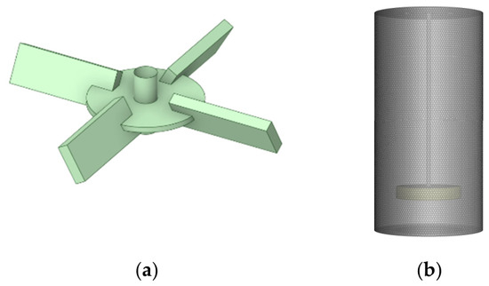
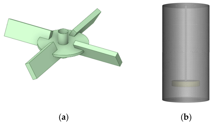
The stirring mechanism is implemented using the Multiple Reference Frame (MRF) method based on the model constructed before. Figure 13 illustrates the structure of the stirrer and the mesh of the reactor with the stirrer. Mittal et al. [45] evaluated the validity of the MRF method using experimental data. Results indicate that models employing MRF can accurately simulate velocity profiles within reactors. Consequently, this method is considered relatively mature and acceptable. Using MRF, the fluid domain is divided into a rotating reference frame and a stationary reference frame. The fluid domain within the directly modeled stirrer region resides in the rotating reference frame, rotating around the reactor axis at various speeds. Adjacent paddle regions are defined as moving walls, rotating with the internal fluid flow. The remainder of the reactor remains in the stationary reference frame. Numerical instability was observed during computation, effectively mitigated by appropriately reducing the relaxation factor. Other model parameters remain consistent with the previously described model.
Figure 13.
Model of the stirrer. (a) Structure of the stirrer; (b) mesh of the reactor with the stirrer.
3.4.2. Internal Conditions of the Reactor with the Stirrer
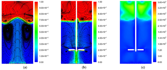
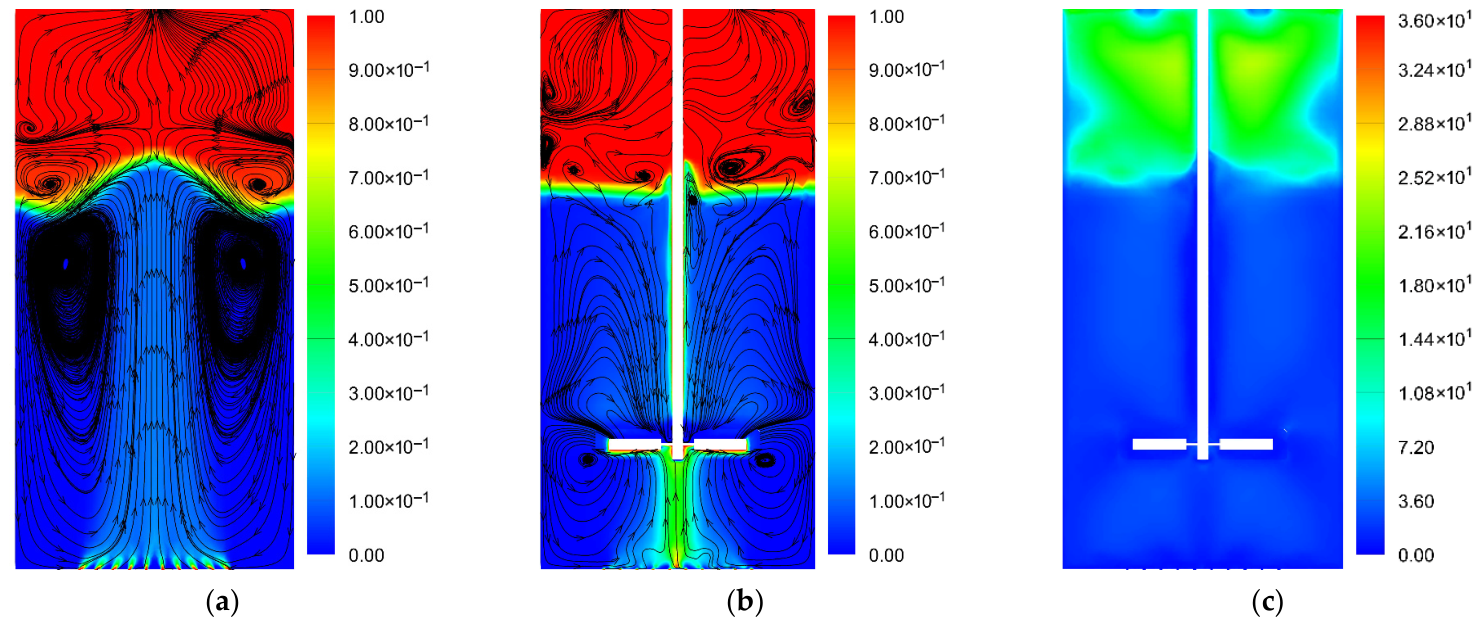
Figure 14 shows the gas volume fraction, steamtraces and the value of Ha in the reactor with and without a stirrer at a rotation speed of 200 rpm. By adding a stirrer, the work amply illustrates the various ways that stirring can improve reactor performance. The gas volume fraction distribution contour clearly shows that the radial distribution of the gas volume fraction in the non-agitated bubble tower is not uniform. The reactor’s center, where the gas level is highest, is where bubbles generate and ascend. Following the introduction of the stirrer, a highly uniform distribution of the gas volume fraction is achieved through the severe shear. The contour displays an almost symmetrical distribution, with the color becoming uniform radially. The streamlines in Figure 14b clearly reveal the forced circulation vortices generated by the stirrer. Below the paddles, gas is drawn into the stirrer zone, sheared and fragmented, then rapidly propelled toward the wall with the liquid flow. It subsequently descends along the wall before being redrawn into the stirrer zone. Bubbles eventually ascend to the fluid surface after several cycles inside the reactor, taking longer routes. This gives the gas phase extra time for dissolution and reaction by extending its average residence time. The vigorous circulation ensures gas flow traces traverse every corner of the reactor, virtually eliminating dead zones and enabling efficient utilization of catalysts throughout all regions. In addition, the stirrer transfers the flow pattern into a more uniform distribution of the gas volume fraction, temperature, and concentration.
Figure 14.
Contours of reactors with/without a stirrer. (a) Gas volume fraction and steamtraces without a stirrer; (b) gas volume fraction and steamtraces with a stirrer; (c) value of Ha with a stirrer.
Figure 14c shows the contours of the Ha value in the axial cross-section of the reactor. The Ha value dropped in the majority of the reactor’s regions, suggesting that the addition of the stirrer lessened the mass transfer restrictions on the reaction. Intense turbulence caused by agitation increases the liquid-phase mass transfer coefficient kL, while microscopic bubbles produce a huge interfacial area. Ultimately, the volumetric mass transfer coefficient increases substantially, and the reactor operating point shifts from a strongly mass transfer-controlled region toward a kinetics-controlled region. This demonstrates that the stirrer serves as a powerful design strategy for overcoming mass transfer bottlenecks.
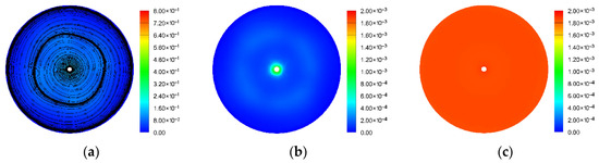
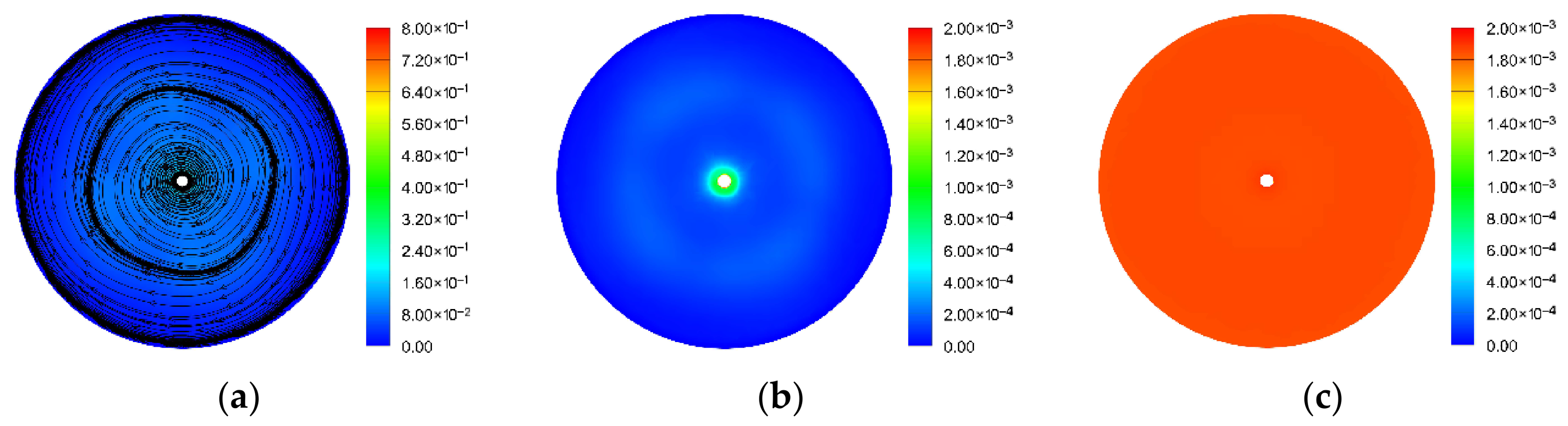
Figure 15 displays the contour plots of the radial gas volume fraction and steamtraces, H2 mass transfer, and n-butyraldehyde formation rate at a reactor height of 0.3 at a rotational speed of 200 rpm. The stirrer is in a clockwise orientation, according to an analysis of the streamline diagrams and gas volume fraction distribution. The evenly dispersed streamlines show high mixing efficiency. The paddle is surrounded by a sizable, clearly defined mass transfer zone, which greatly improves overall mass transfer efficiency.
Figure 15.
Contour plots of the reactor’s radial cross-section at 200 rpm. (a) Gas volume fraction and steamtraces; (b) mass transfer rate of H2 (kg/m3s); (c) reaction rate of n-butyraldehyde (kg/m3s).
3.4.3. Influence of the Speed
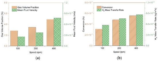
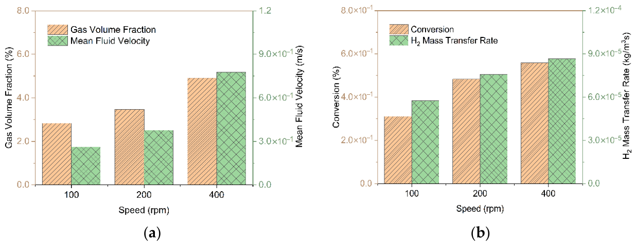
Figure 16 shows the gas volume fraction (volume-averaged below the z/H = 0.6), mean fluid velocity, conversion rate, and H2 mass transfer rate within the reactor at different rotational speeds. Figure 16a shows that increasing the stirring speed significantly enhances both the gas volume fraction and the average liquid-phase velocity. The elevated gas volume fraction indicates prolonged bubble residence time. Meanwhile, the increased average liquid-phase velocity signifies greater turbulence, which is beneficial for mass transfer. As seen in Figure 16b, both the mass transfer rate and conversion exhibit varying degrees of increase. Conversion rates increased by 19% after the optimization.
Figure 16.
Parameters of reactors at different stirring speeds. (a) Gas volume fraction and mean fluid velocity; (b) conversion and H2 mass transfer rate (kg/m3s).
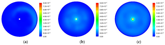
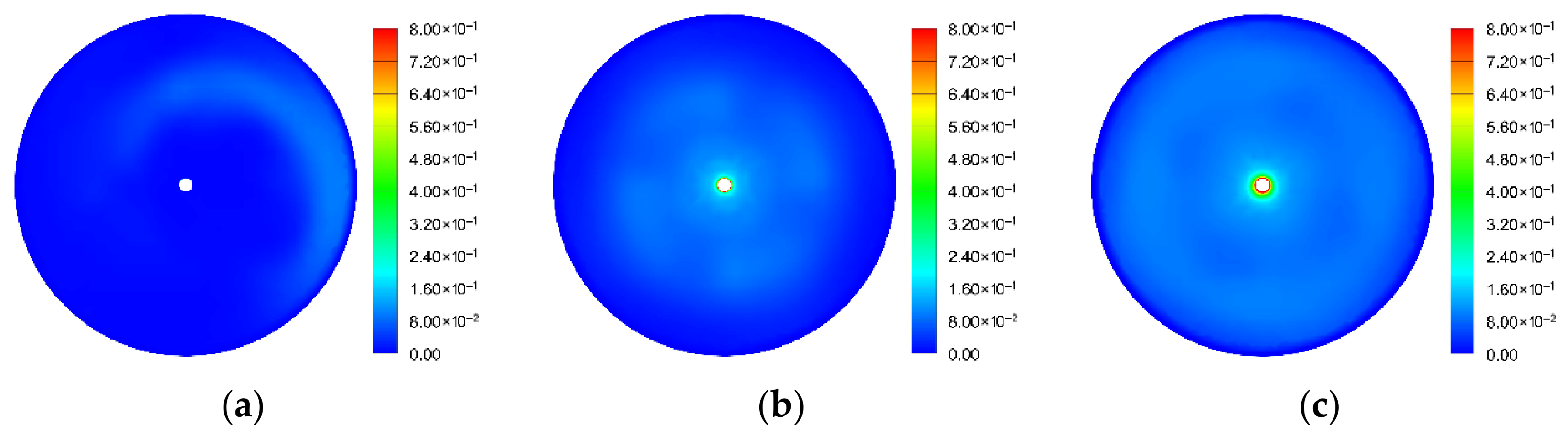
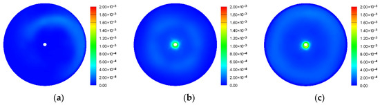
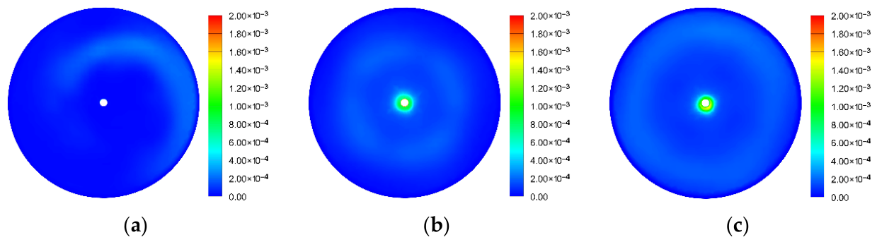
Figure 17 and Figure 18 show the gas–liquid-phase fraction and mass transfer contour plots at the reactor radial position (z/H = 0.3) under different rotational speeds. High stirring speed increases mass transfer and reaction rates to varying degrees and greatly increases the gas volume fraction rate. Large bubbles added to the system are effectively broken up into a large number of uniformly fine microbubbles by the shear. Shear forces are stronger with higher stirring rates. While the size of the bubbles reduces with increasing rotational speed, the number of bubbles increases, thus improving the mass transfer. Strong agitation creates extremely turbulent liquid flow, which lowers the thickness of the liquid film and raises the liquid-phase mass transfer coefficient. As a result, the total volumetric mass transfer coefficient is much higher. This significantly reduces mass transfer constraints by facilitating the quicker solubility of CO and H2 and their transport to catalyst active sites. Higher mass transfer rates provide more supply of reactants, raise liquid phase reactant concentrations, and ultimately increase the macroscopic reaction rate. Additionally, stirring ensures uniform distribution throughout the field, which facilitates higher conversion rates while lessening the load on subsequent separation processes. It also minimizes potential local hot spots or regions of excessively low reactant concentration in the bubble column. This lessens the likelihood of related adverse reactions and promotes greater reactor stability.
Figure 17.
Radial gas volume fraction contours at different rotational speeds. (a) 100 rpm; (b) 200 rpm; (c) 400 rpm.
Figure 18.
Radial mass transfer contours at different rotational speeds. (a) 100 rpm; (b) 200 rpm; (c) 400 rpm.
Therefore, selecting an appropriate stirring speed is a key factor in enhancing reactor performance. Additionally, optimizing the stirring structure, such as designing multi-blade impellers, is also an effective approach. Reasonable reactor design and selection depend on accurately assessing the reaction’s rate-determining step and selecting the right optimizing operating conditions.
4. Conclusions
This work establishes a three-dimensional CFD-PBM coupled model to simulate fluid flow, mass transfer, and reaction processes within a gas–liquid reactor for the hydroformylation of propylene. The main conclusions are summarized as follows:
- The findings show that the gas–liquid reactor’s flow field, mass transfer, and reaction are intimately related and have an impact on each other. The three-dimensional CFD-PBM coupled model is an indispensable tool for accurately capturing the intrinsic mechanisms of such complex systems. The complicated behavior inside the reactor can be more theoretically supported with the use of CFD techniques.
- Through a visualized Ha contour, we have overcome the limitations of traditional point analysis or global averaging, confirming that under typical operating conditions, 65% of the reaction area in the propylene hydroformylation reactor is mass transfer-limited. Since the reaction is primarily mass transfer-controlled, this guides our subsequent optimization.
- Reactor performance can be effectively improved under current operating circumstances by boosting the system pressure. The conversion rate almost doubles when the pressure is increased. Appropriately increasing the superficial gas velocity is also beneficial for reaction enhancement. The conversion rate rises by 23% as the apparent gas velocity doubles. However, there is a critical point beyond which the reactor’s flow pattern drastically alters. The critical value in the current model is a superficial gas velocity of 0.02 m/s. Certain parameters need more research because of things like scale-up effects in real reactors.
- Reactor performance is significantly impacted by structural design. Reactor performance can be enhanced and mass transfer restrictions can be reduced using the stirrer. For better reaction efficiency, the agitation speed needs to be adjusted. The conversion rate in the current model can be increased by 19% by running at 400 rpm.
In conclusion, these discoveries not only enhance our comprehension of the complex processes taking place in gas–liquid reactors but also offer a quantitative theoretical foundation and precise recommendations for the intended design and operational optimization of industrial gas–liquid reactors.
Author Contributions
Conceptualization, L.M. and Z.G.; methodology, Z.G.; software, L.M.; validation, B.W., J.M. and J.Z.; formal analysis, L.M.; investigation, Z.G.; resources, J.M.; data curation, B.W.; writing—original draft preparation, L.M.; writing—review and editing, Z.G.; visualization, B.W.; supervision, Z.G.; project administration, Z.G.; funding acquisition, J.M. All authors have read and agreed to the published version of the manuscript.
Funding
This research received no external funding.
Data Availability Statement
The original contributions presented in this study are included in the article. Further inquiries can be directed to the corresponding author.
Acknowledgments
The authors have reviewed and edited the output and take full responsibility for the content of this publication.
Conflicts of Interest
The authors declare no conflicts of interest.
Abbreviations
The following abbreviations are used in this manuscript:
| CBSM | Constant Bubble Size Modeling Approach |
| CFD | Computational Fluid Dynamics |
| CFL | Courant–Friedrichs–Lewy |
| PBM | Population Balance Model |
| RNG | Renormalization Group |
| VBSM | Variable Bubble Size Modeling Approach |
References
- Fan, B.; Jiang, M.; Wang, G.; Zhao, Y.; Mei, B.; Han, J.; Ma, L.; Li, C.; Hou, G.; Wu, T.; et al. Elucidation of hemilabile-coordination-induced tunable regioselectivity in single-site Rh-catalyzed heterogeneous hydroformylation. Nat. Commun. 2024, 15, 6967. [Google Scholar] [CrossRef] [Scilit] [PubMed]
- Alvarado Rupflin, L.; Mormul, J.; Lejkowski, M.; Titlbach, S.; Papp, R.; Gläser, R.; Dimitrakopoulou, M.; Huang, X.; Trunschke, A.; Willinger, M.G.; et al. Platinum Group Metal Phosphides as Heterogeneous Catalysts for the Gas-Phase Hydroformylation of Small Olefins. ACS Catal. 2017, 7, 3584–3590. [Google Scholar] [CrossRef] [Scilit]
- Ungváry, F. Application of transition metals in hydroformylation annual survey covering the year 2003. Coord. Chem. Rev. 2004, 248, 867–880. [Google Scholar] [CrossRef] [Scilit]
- Manzano, M.H.; Poissonnier, J.; Siradze, S.; Thybaut, J.W. Liquid versus gas-phase operation in heterogeneously catalyzed hydroformylation. Chem. Eng. J. 2025, 506, 159766. [Google Scholar] [CrossRef] [Scilit]
- Yan, P.; Jin, H.; He, G.; Guo, X.; Ma, L.; Yang, S.; Zhang, R. Numerical simulation of bubble characteristics in bubble columns with different liquid viscosities and surface tensions using a CFD-PBM coupled model. Chem. Eng. Res. Des. 2020, 154, 47–59. [Google Scholar] [CrossRef] [Scilit]
- Franke, R.; Selent, D.; Börner, A. Applied Hydroformylation. Chem. Rev. 2012, 112, 5675–5732. [Google Scholar] [CrossRef] [Scilit] [PubMed]
- Rossetti, I.; Compagnoni, M. Chemical reaction engineering, process design and scale-up issues at the frontier of synthesis: Flow chemistry. Chem. Eng. J. 2016, 296, 56–70. [Google Scholar] [CrossRef] [Scilit]
- Jamshidian, R.; Scully, J.; Van Den Akker, H.E.A. A computational fluid dynamics study of mass transfer in a large-scale aerated stirred bioreactor. Chem. Eng. J. 2025, 509, 160723. [Google Scholar] [CrossRef] [Scilit]
- Taborda, M.A.; Sommerfeld, M. Reactive LES-Euler/Lagrange modelling of bubble columns considering effects of bubble dynamics. Chem. Eng. J. 2021, 407, 127222. [Google Scholar] [CrossRef] [Scilit]
- Amaral, A.; Bellandi, G.; Rehman, U.; Neves, R.; Amerlinck, Y.; Nopens, I. Towards improved accuracy in modeling aeration efficiency through understanding bubble size distribution dynamics. Water Res. 2018, 131, 346–355. [Google Scholar] [CrossRef] [Scilit]
- Chen, S.; Lang, X.; Kourou, A.; Dutta, S.; Van Geem, K.M.; Ouyang, Y.; Heynderickx, G.J. Enhancing CO2 capture efficiency: Computational fluid dynamics investigation of gas-liquid vortex reactor configurations for process intensification. Chem. Eng. J. 2024, 493, 152535. [Google Scholar] [CrossRef] [Scilit]
- Liu, J.; Zhou, P.; Liu, L.; Chen, S.; Song, Y.; Yan, H. CFD modeling of reactive absorption of CO2 in aqueous NaOH in a rectangular bubble column: Comparison of mass transfer and enhancement factor model. Chem. Eng. Sci. 2021, 230, 116218. [Google Scholar] [CrossRef] [Scilit]
- Zhao, L.; Sun, Q.; Tang, Z. Multi-phase CFD modelling for hydroformylation of 1-hexene with microbubbles. Chem. Eng. Process.-Process Intensif. 2022, 181, 109163. [Google Scholar] [CrossRef] [Scilit]
- Darmana, D.; Deen, N.G.; Kuipers, J.A.M. Detailed modeling of hydrodynamics, mass transfer and chemical reactions in a bubble column using a discrete bubble model. Chem. Eng. Sci. 2005, 60, 3383–3404. [Google Scholar] [CrossRef] [Scilit]
- Ngu, V.; Morchain, J.; Casale, B.; Cockx, A. Modelling of biological methanation by CFD and 1D model in an industrial bubble column. Chem. Eng. Sci. 2025, 316, 121940. [Google Scholar] [CrossRef] [Scilit]
- Tao, X.; Qi, H.; Guo, Z.; Wang, J.; Wang, X.; Yang, J.; Zhao, Q.; Lin, W.; Yang, K.; Chen, C. Assessment of Measured Mixing Time in a Water Model of Eccentric Gas-Stirred Ladle with a Low Gas Flow Rate: Tendency of Salt Solution Tracer Dispersions. Symmetry 2024, 16, 1241. [Google Scholar] [CrossRef] [Scilit]
- Varela, S.; Martínez, M.; Delgado, J.A.; Godard, C.; Curulla-Ferré, D.; Pallares, J.; Vernet, A. Numerical and experimental modelization of the two-phase mixing in a small scale stirred vessel. J. Ind. Eng. Chem. 2018, 60, 286–296. [Google Scholar] [CrossRef] [Scilit]
- Breit, F.; Hofmann, M.; Kharik, E.; von Harbou, E. Sensitivity and Parameter Analysis of a Population Balance Model Applied to Non-Reactive Gas–Liquid Semi-Batch Perfectly Stirred Tank Reactors. Chem. Eng. Sci. 2026, 327, 123479. [Google Scholar] [CrossRef] [Scilit]
- Shen, T.; Lu, D.; Liu, Z.; Chen, R.; Gong, M. Heat and mass transfer performance analysis of a vertical tubular ammonia/water bubble absorber based on CFD modeling. Appl. Therm. Eng. 2024, 252, 123622. [Google Scholar] [CrossRef] [Scilit]
- Zhu, L.T.; Chen, X.Z.; Ouyang, B.; Yan, W.-C.; Lei, H.; Chen, Z.; Luo, Z.-H. Review of Machine Learning for Hydrodynamics, Transport, and Reactions in Multiphase Flows and Reactors. Ind. Eng. Chem. Res. 2022, 61, 9901–9949. [Google Scholar] [CrossRef] [Scilit]
- Gaurav, T.K.; Prakash, A.; Zhang, C. CFD modeling of the hydrodynamic characteristics of a bubble column in different flow regimes. Int. J. Multiph. Flow 2022, 147, 103902. [Google Scholar] [CrossRef] [Scilit]
- Van Wachem, B.G.M.; Almstedt, A.E. Methods for multiphase computational fluid dynamics. Chem. Eng. J. 2003, 96, 81–98. [Google Scholar] [CrossRef] [Scilit]
- Laborde-Boutet, C.; Larachi, F.; Dromard, N.; Delsart, O.; Schweich, D. CFD simulation of bubble column flows: Investigations on turbulence models in RANS approach. Chem. Eng. Sci. 2009, 64, 4399–4413. [Google Scholar] [CrossRef] [Scilit]
- Fletcher, D.F.; Mcclure, D.D.; Kavanagh, J.M.; Barton, G.W. CFD simulation of industrial bubble columns: Numerical challenges and model validation successes. Appl. Math. Model. 2017, 44, 25–42. [Google Scholar] [CrossRef] [Scilit]
- Troshko, A.A.; Hassan, Y.A. A two-equation turbulence model of turbulent bubbly flows. Int. J. Multiph. Flow 2001, 27, 1965–2000. [Google Scholar] [CrossRef] [Scilit]
- Larachi, F.; Desvigne, D.; Donnat, L.; Schweich, D. Simulating the effects of liquid circulation in bubble columns with internals. Chem. Eng. Sci. 2006, 61, 4195–4206. [Google Scholar] [CrossRef] [Scilit]
- Delnoij, E.; Lammers, F.A.; Kuipers, J.A.M.; van Swaaij, W. Dynamic simulation of dispersed gas-liquid two-phase flow using a discrete bubble model. Chem. Eng. Sci. 1997, 52, 1429–1458. [Google Scholar] [CrossRef] [Scilit]
- Odar, F.; Hamilton, W.S. Forces on a sphere accelerating in a viscous fluid. J. Fluid Mech. 1964, 18, 302–314. [Google Scholar] [CrossRef] [Scilit]
- Tomiyama, A.; Tamai, H.; Zun, I.; Hosokawa, S. Transverse migration of single bubbles in simple shear flows. Chem. Eng. Sci. 2002, 57, 1849–1858. [Google Scholar] [CrossRef] [Scilit]
- Yang, G.; Zhang, H.; Luo, J.; Wang, T. Drag force of bubble swarms and numerical simulations of a bubble column with a CFD-PBM coupled model. Chem. Eng. Sci. 2018, 192, 714–724. [Google Scholar] [CrossRef] [Scilit]
- Varallo, N.; Besagni, G.; Mereu, R. Computational fluid dynamics simulation of the heterogeneous regime in a large-scale bubble column. Chem. Eng. Sci. 2023, 280, 119090. [Google Scholar] [CrossRef] [Scilit]
- Gemello, L.; Cappello, V.; Augier, F.; Marchisio, D.; Plais, C. CFD-based scale-up of hydrodynamics and mixing in bubble columns. Chem. Eng. Res. Des. 2018, 136, 846–858. [Google Scholar] [CrossRef] [Scilit]
- Khalil, A.; Rosso, D.; Degroot, C.T. Effects of flow velocity and bubble size distribution on oxygen mass transfer in bubble column reactors—A critical evaluation of the computational fluid dynamics-population balance model. Water Environ. Res. 2021, 93, 2274–2297. [Google Scholar] [CrossRef] [Scilit]
- Wang, T.; Wang, J. Numerical simulations of gas–liquid mass transfer in bubble columns with a CFD–PBM coupled model. Chem. Eng. Sci. 2007, 62, 7107–7118. [Google Scholar] [CrossRef] [Scilit]
- Guo, K.; Wang, T.; Liu, Y.; Wang, J. CFD-PBM simulations of a bubble column with different liquid properties. Chem. Eng. J. 2017, 329, 116–127. [Google Scholar] [CrossRef] [Scilit]
- Luo, H.; Svendsen, H.F. Theoretical model for drop and bubble breakup in turbulent dispersions. AIChE J. 1996, 42, 1225–1233. [Google Scholar] [CrossRef] [Scilit]
- Syed, A.H.; Boulet, M.; Melchiori, T.; Lavoie, J.-M. CFD Simulations of an Air-Water Bubble Column: Effect of Luo Coalescence Parameter and Breakup Kernels. Front. Chem. 2017, 5, 68. [Google Scholar] [CrossRef] [Scilit] [PubMed]
- Bernas, A.; Wärnå, J.; Mäki-Arvela, P.; Murzin, D.Y.; Salmi, T. Kinetics and mass transfer in hydroformylation—Bulk or film reaction? Can. J. Chem. Eng. 2010, 88, 618–624. [Google Scholar] [CrossRef] [Scilit]
- Bernas, A.; Mäki-Arvela, P.; Lehtonen, J.; Salmi, T.; Murzin, D.Y. Kinetic Modeling of Propene Hydroformylation with Rh/TPP and Rh/CHDPP Catalysts. Ind. Eng. Chem. Res. 2008, 47, 4317–4324. [Google Scholar] [CrossRef] [Scilit]
- Shaharun, M.S.; Mukhtar, H.; Dutta, B.K. Solubility of carbon monoxide and hydrogen in propylene carbonate and thermomorphic multicomponent hydroformylation solvent. Chem. Eng. Sci. 2008, 63, 3024–3035. [Google Scholar] [CrossRef] [Scilit]
- Wilke, C.R.; Chang, P. Correlation of diffusion coefficients in dilute solutions. AIChE J. 1955, 1, 264–270. [Google Scholar] [CrossRef] [Scilit]
- Zhang, H.; Guo, K.; Wang, Y.; Sayyar, A.; Wang, T. Numerical simulations of the effect of liquid viscosity on gas-liquid mass transfer of a bubble column with a CFD-PBM coupled model. Int. J. Heat Mass Transf. 2020, 161, 120229. [Google Scholar] [CrossRef] [Scilit]
- Shi, W.; Yang, N.; Yang, X. A kinetic inlet model for CFD simulation of large-scale bubble columns. Chem. Eng. Sci. 2017, 158, 108–116. [Google Scholar] [CrossRef] [Scilit]
- Dhotre, M.; Joshi, J. Design of a gas distributor: Three-dimensional CFD simulation of a coupled system consisting of a gas chamber and a bubble column. Chem. Eng. J. 2007, 125, 149–163. [Google Scholar] [CrossRef] [Scilit]
- Mittal, G.; Issao Kikugawa, R. Computational fluid dynamics simulation of a stirred tank reactor. Mater. Today Proc. 2021, 46, 11015–11019. [Google Scholar] [CrossRef] [Scilit]



Disclaimer/Publisher’s Note: The statements, opinions and data contained in all publications are solely those of the individual author(s) and contributor(s) and not of MDPI and/or the editor(s). MDPI and/or the editor(s) disclaim responsibility for any injury to people or property resulting from any ideas, methods, instructions or products referred to in the content. |
© 2026 by the authors. Licensee MDPI, Basel, Switzerland. This article is an open access article distributed under the terms and conditions of the Creative Commons Attribution (CC BY) license.