


Abstract
To accurately quantify pore pressure uncertainty and associated kick risk, this paper proposes a dual-phase pre-drilling risk assessment framework based on Bayesian Long Short-Term Memory (BLSTM) networks, integrating formation pressure prediction with distribution interference analysis. First, the effects of two Bayesian layer optimization methods—Monte Carlo dropout and Bayes-by-Backprop—on deep learning networks were systematically evaluated. The optimized Bayes-by-Backprop-LSTM model was subsequently selected for uncertainty prediction of formation pore pressure. Finally, kick risk was quantified by analyzing the interference between predicted pressure distributions and the safety margin of designed drilling mud density. The BLSTM models uncertainty regression between well-log parameters and formation pore pressure labels. Using the Bayes-by-Backprop strategy, it generates probabilistic pressure predictions. By incorporating the designed drilling mud density of target wells, kick risk probability is calculated through distribution interference criteria, where the overlapping area between pore pressure distributions and mud density safety boundaries is mapped to risk probability. Validation experiments utilized five types of well-log parameters from three wells in EAST CHINA. Key results demonstrate: (1) The BLSTM regression model achieved a mean absolute error (MAE) of 0.037 on test wells, representing a 26.7% reduction compared to conventional LSTM, with the 95% confidence interval coverage reaching 69.6%. (2) In the 3893–4048 m interval of a test well, interference areas exceeding thresholds indicated 60% kick risk probability. Spatial correlation with actual kick events revealed risk points undetectable by conventional pore pressure prediction methods. This study establishes a comprehensive risk assessment paradigm encompassing pore pressure uncertainty regression prediction and probabilistic risk calculation, providing drilling engineering with a framework that combines physical interpretability and statistical reliability.
1. Introduction
Drilling safety is paramount in oil and gas operations, with kick incidents being a primary precursor to catastrophic blowouts. As exploration extends into deeper and more geologically complex formations, the inherent and significant uncertainties in formation pressure prediction have become a central bottleneck for reliable kick risk assessment. Traditional deterministic assessment methods often struggle to provide actionable insights under such conditions, necessitating a paradigm shift in risk evaluation—from deterministic safety-margin checks towards a probabilistic analysis that explicitly quantifies these uncertainties.
Kick risk assessment primarily encompasses two approaches: (1) Pre-drilling calculation of formation pore pressure to evaluate whether the designed drilling mud equivalent density meets safety requirements and to identify strata with elevated kick risks. (2) Real-time monitoring of abnormal fluctuations in logging parameters during drilling to detect early kick indicators.
In pore pressure prediction, Rashidi et al. [1] employed artificial neural networks (ANN) to map mechanical specific energy (MSE) and drilling efficiency (DE) to pore pressure, achieving real-time pressure prediction while drilling with a high test-set correlation coefficient of R ≈ 0.996. Abdulmalek et al. [2] utilized fuzzy logic to integrate drilling parameters and logging data for pore pressure prediction, attaining R = 0.998 and mean absolute error < 0.24%. Hadi et al. [3] implemented regression analysis and ANN using conventional well logs to predict pore pressure in carbonate depleted reservoirs, achieving R2 = 0.96—significantly outperforming traditional Eaton and Ratio methods. Sun et al. [4] applied a multi-mechanism modified Bowers model incorporating shale content with loading/unloading dual mechanisms for abnormal high-pressure formation prediction, reducing maximum error by ~20% and average error to ~3%. Cao et al. [5] developed a knowledge-aware temporal fusion transformer (TFT) deep model for time-series pore pressure forecasting, achieving R2 = 0.997, RMSE = 0.135 MPa, and uncertainty quantification.
Engineers typically monitor and analyze logging data for real-time kick risk assessment. Zhang et al. [6] proposed a DBSCAN clustering-based method for kick feature identification and monitoring in fractured-vuggy carbonate reservoirs, establishing a top-down logical framework for early kick detection through four-tier classification to recommend intervention measures. Wu et al. [7] introduced an ensemble learning model integrating Stacking and Bagging algorithms for kick risk diagnosis, fusing multiple time-series analysis methods to optimize diagnostic models for comprehensive risk evaluation.
Although AI methods demonstrate high accuracy in point prediction of pore pressure, these models largely operate within a deterministic prediction paradigm, optimized to output a single value by precisely fitting target labels. This paradigm fails to quantify the uncertainties arising from geological variability, data noise, and model structure, thereby limiting the reliability assessment of predictions under new blocks or complex geological conditions. Consequently, quantifying risk uncertainty to provide probabilistic assessments, rather than point estimates, enables engineers to holistically understand geological risks, identify latent precursors, and optimize engineering solutions and contingency plans.
Quantifying uncertainties arising from geological factors, measurement limitations, and field equipment facilitates scientifically rigorous risk assessment. Whittaker et al. [8] pioneered a Markov chain model in 2000 for predicting multi-structure software reliability, establishing mathematical foundations for subsequent models. Langseth [9] demonstrated in 2007 that Bayesian networks (BN) are particularly suited for system reliability analysis, now widely adopted in risk assessment.
Traditional risk assessment techniques fail to capture dynamic operational impacts, whereas well control incidents (loss, kick, blowout) exhibit time-dependent characteristics. Cai et al. [10] addressed this in 2013 using dynamic Bayesian networks (DBN)—temporal extensions of BN—for dynamic risk modeling. Building on this, Wu et al. [11] applied DBN to predict and diagnose drilling accidents. To accommodate varying fault tree structures across drilling phases, Shi [12] implemented structure-variable DBN (SVDBN) for dynamic risk structure adaptation, specifically modeling risks from in situ natural gas hydrate formation.
Regarding measurement uncertainty, scholars have explored quantifying raw data uncertainty to assess risk probabilistically. Guan et al. [13] identified in 2013 that uncertainties in wellbore design parameters may induce drilling risks, developing a probabilistic assessment method integrating interval analysis and reliability theory with downhole complexity factors. Sheng [14] established in 2019 a quantification framework for geomechanically parameters with uncertainty, deriving formation pressure distributions via Monte Carlo simulation to create a risk characterization system. Xu et al. [15] addressed unevenly distributed historical wells in offshore fields by constructing virtual wells based on seismic velocity-rock mechanics relationships in 2023, using LSTM models to predict risk profiles and significantly enhance regional uncertainty assessment. Pore pressure uncertainty quantification reveals latent geological risks.
Although dynamic uncertainty networks have been successfully applied to real-time risk monitoring and dynamic accident analysis, these methods have not yet integrated uncertainty quantification capabilities with advanced deep learning models for pre-drilling pore pressure prediction. Existing uncertainty analyses predominantly rely on traditional physical or statistical methods, failing to fully leverage the ability of deep learning to capture complex non-linear patterns from extensive well-logging data. Consequently, current pre-drilling risk assessments struggle to effectively quantify the inherent variability of geological parameters and their contribution to pressure prediction uncertainty. This study aims to bridge this gap by introducing an uncertainty-quantifying neural network, transforming pre-drilling pore pressure prediction from a deterministic output into a probabilistic assessment capable of revealing latent geological risk factors.
This study proposes an uncertainty-quantifying neural network optimized via Monte Carlo dropout and Bayes-by-Backprop mechanisms. The model accepts acoustic slowness, bulk density, compensated neutron logs, and other parameters as inputs to generate pore pressure predictions with confidence intervals. We comparatively evaluate optimized BP neural networks and LSTM architectures for formation pressure prediction performance, ultimately selecting the optimal model for kick risk assessment integrated with engineering design parameters. The probabilistic risk output is then integrated with design mud weight windows through a distribution interference approach, generating quantitative risk profiles along the wellbore to support optimized drilling design decisions. This enables comparative safety evaluation of multiple design scenarios during the planning phase, facilitating data-driven optimization of well control strategies. By enabling efficient uncertainty quantification, this research transforms kick risk evaluation from deterministic safety-margin checks to probabilistic risk analysis, uncovering latent hazards to enhance drilling safety.
2. Theory
2.1. Monte Carlo Dropout Layers
Monte Carlo Dropout (MC Dropout) serves as an efficient Bayesian approximation method that reinterprets dropout techniques in deep learning to provide a principled uncertainty quantification framework for neural networks. Conventional dropout randomly “deactivates” neurons during training to prevent overfitting, while deterministically scaling activation values during testing. The key innovation of MC Dropout lies in reinterpreting dropout behavior at test time as approximate sampling from the Bayesian posterior distribution. From a Bayesian perspective, the posterior distribution A of neural network weights can be approximated via dropout after given dataset . Specifically, during each forward propagation, we apply a Bernoulli mask to every unit within the network:
In the equation, denotes the activation value of the -th layer, represents the masking vector following a Bernoulli distribution, and signifies the retention probability. Through multiple forward propagation iterations with retention and dropout operations, we effectively sample from the approximate posterior distribution.
The theoretical connection between MC Dropout and variational inference was demonstrated by Gal and Ghahramani [16,17], who showed that neural networks employing dropout correspond to specific variational approximations of Bayesian posteriors. Specifically, the variational distribution corresponding to dropout is
In the equation, denotes the Bernoulli mask matrix and represents the deterministic weights. Through this approximation, the model’s predictive distribution can be estimated via Monte Carlo integration:
In the equation, denotes the number of forward propagation iterations, and represents the weight configuration at the -th sampling point.
2.2. Bayes by Backprop Weight Layer
This paper further incorporates a Bayesian layer based on Bayes by Backprop [18,19] into the model architecture to introduce uncertainty into the weight layer. Bayes by Backprop is an efficient Bayesian learning algorithm that models weight uncertainty by learning the probability distribution of neural network weights through minimizing the variational free energy.
Bayesian neural networks provide a principled solution to these problems by treating weights as random variables rather than deterministic values.
The core idea involves specifying a prior distribution for the weight parameters, then computing the posterior distribution given training data via Bayes’ theorem:
In the equation, denotes the likelihood function, and represents the evidence term. However, for complex neural network models, the computation of the posterior distribution involves high-dimensional integration, which is typically difficult to solve directly. Therefore, the weights of the neural network are treated as random variables, assumed to follow a variational distribution , where denotes the variational parameters. These variational parameters are optimized by minimizing the Kullback–Leibler (KL) divergence between the variational distribution and the true posterior distribution. The optimization objective can be expressed as
This optimization objective is equivalent to maximizing the Evidence Lower Bound (ELBO):
Taking the negative of this formula yields the optimization objective for the neural network:
The first term represents the KL divergence between the prior distribution and the variational distribution , termed the complexity cost; the second term denotes the expected log-likelihood of the data, termed the likelihood cost, which measures the model’s fit to the data. By optimizing this objective function, the model is constrained by the prior distribution while fitting the data, thereby preventing overfitting.
2.3. BP Model
The Back Propagation (BP) neural network is a common type of neural network. It is a multi-layer feedforward neural network trained using the error backpropagation algorithm. The structure of a BP neural network comprises an input layer, hidden layers, and an output layer, where the hidden layer may consist of one or multiple layers. Neurons within the same layer are fully connected, whilst there are no connections between neurons across different layers.
Let the input vector of the BP neural network be , and the desired output vector be . During the forward propagation process, the input and output calculations for the hidden layer are as follows:
Hidden layer input calculation:
In the equation, denotes the input to the -th neuron in the hidden layer, represents the connection weight from the -th neuron in the input layer to the -th neuron in the hidden layer, and is the -th element of the input vector.
Hidden layer output calculation:
In the equation, denotes the output of the -th neuron in the hidden layer, represents the activation function, and signifies the threshold of the -th neuron in the hidden layer.
Output layer input calculation:
In the equation, denotes the input to the -th neuron in the output layer, represents the connection weight from the -th neuron in the hidden layer to the -th neuron in the output layer, and signifies the number of neurons in the hidden layer.
Output layer output calculation:
In the equation, denotes the actual output of the -th neuron in the output layer, and denotes the threshold of the -th neuron in the output layer. For a training sample , where the network’s actual output is , the network’s mean squared error is
In the equation, denotes the error of the -th sample, and represents the -th element of the desired output.
The BP algorithm, based on gradient descent, adjusts network parameters by calculating the partial derivatives of the error function with respect to each parameter. The core formula for weight adjustment is
In the formula, denotes the learning rate, which controls the step size for parameter updates.
2.4. LSTM Model
Long Short-Term Memory (LSTM) neural networks are a specialized type of recurrent neural network (RNN) suited to processing contextual dependencies within long sequence data. They overcome the shortcomings of standard RNNs, such as gradient vanishing, exploding gradients, and difficulty in maintaining long-term memory.
LSTM networks exhibit significant advantages over Fully Connected Neural Networks (FNN) in this field, primarily due to their ability to effectively capture the temporal dependencies within logging data along the depth domain. The processes of stratum sedimentation and evolution are inherently sequential and nonlinear, resulting in variations in logging parameters with depth that are not independent but rather contain crucial geological contextual information. In contrast, a fully connected network treats data from each depth point as an independent sample, failing to model such sequential correlations. Consequently, it struggles to identify features characterized by long-term dependencies, such as abnormal pressure transition zones.
The LSTM unit possesses extended short-term memory capabilities through gating mechanisms comprising a forget gate (f), an input gate (i), and an output gate (o). The forget gate governs whether information from the cell’s previous state Ct-1 should be retained or discarded.
Here, denotes the output from the previous stage, represents the input at the current stage, and is the sigmoid activation function. Input gate: Determines which information to incorporate based on the current input and the hidden state of the memory cell from the previous time step. Decides how much of the important information in vector to retain. is obtained via the sigmoid function, is derived from the tanh function, and the state is updated according to Equation (17).
Here, and denote the weight and bias vectors for the sigmoid layer, respectively; and denote the weight and bias vectors for the tanh layer respectively.
The output gate sigmoid activation function determines the features characterizing the output cell’s state:
In which and are the parameters of the output gate.
Applying the tanh function to and multiplying the result by the vector yields .
Within the geological settings of typical oilfield blocks, strata exhibit vertical distribution through sedimentary sequences, with their depositional patterns and corresponding logging curves displaying pronounced sequentially. Given the relatively stable depositional environment in the target block, employing LSTM to learn the sequential characteristics of logging curves in the depth domain may prove more advantageous for parameter prediction.
3. Data Processing
3.1. Data Description
The proposed methodology was validated using data from three exploration wells in an oilfield block in eastern China. Each well provided five types of conventional logging curves: acoustic log (AC), gamma ray (GR), spontaneous potential (SP), density log (DEN), and compensated neutron log (CN). The vertical sampling interval for all curves was 0.2 m. After filtering valid intervals and parameters, the depth ranges and data allocation for the three wells are summarized in Table 1. Based on data volume and historical records, Wells A1 and A2 were designated as the training set, while Well A3—with sufficient data and documented kick incidents—served as the test set to evaluate model accuracy and risk assessment performance.
Table 1.
Data overview.
Additionally, the designed drilling mud density profiles for all three wells were acquired to assess kick risk after pore pressure prediction. The mud density data shared the same vertical sampling interval of 0.2 m.
3.2. Data Preprocessing
3.2.1. Outlier Removal
To ensure data consistency, all logging curves and drilling mud density data were aligned in depth and subjected to preprocessing, including outlier removal, trend elimination, and standardization. In sequential data processing, outliers can significantly compromise analytical accuracy. This study employs a sliding-window Interquartile Range (IQR) method for outlier detection, which offers enhanced robustness for non-normally distributed data. The IQR is defined as the difference between the upper quartile () and lower quartile ():
where and represent the 75th and 25th percentiles of the dataset, respectively. Outlier thresholds are determined by scaling the IQR with an adjustable coefficient :
Here, is typically set to 1.5 (for moderate outliers) or 3 (for extreme outliers). The default configuration uses = 1.5, classifying data points below above outliers within each sliding window.
To adapt to local characteristics of the time series, a dynamic sliding window mechanism is implemented. For a sequence of length n, the detection window for each data point covers , where denotes the window radius (default: 50). The window size automatically adjusts at sequence boundaries to maintain valid data coverage, ensuring consistent evaluation of endpoints. This approach requires no prior assumptions about data distribution and effectively identifies localized anomalies.
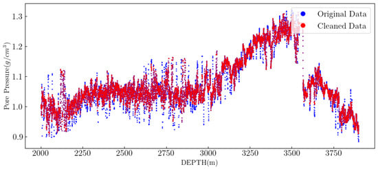
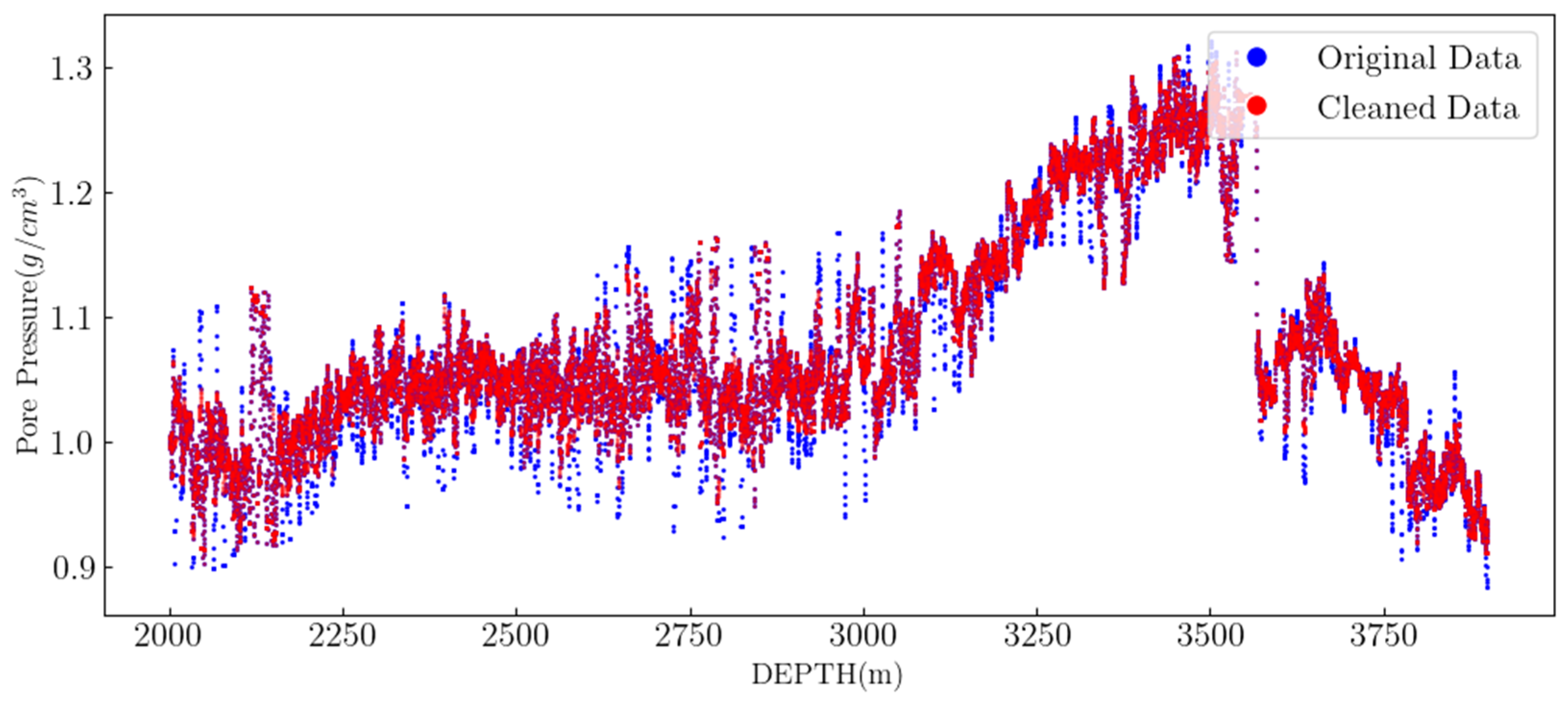
Detected outliers are replaced with Nan values and interpolated linearly using SciPy(1.11)’s interp1dfunction. The interpolation constructs piecewise linear functions based on valid data points adjacent to outliers, preserving global trends while mitigating information loss from direct deletion. The noise reduction effect is shown in Figure 1. This process maintains sequence continuity and supports subsequent analytical reliability.
Figure 1.
Data cleaning example.
3.2.2. Signal Smoothing Processing
After outlier cleaning, the data may still contain high-frequency noise. This study employs a wavelet threshold denoising method for signal smoothing. Wavelet transform decomposes signals into subbands of different frequencies, suppressing noise-dominated high-frequency components through threshold processing. The algorithm first performs wavelet decomposition on the signal.
In the formula, denotes the input signal, wavelet represents the wavelet basis type (default ‘db4’), denotes the number of decomposition levels (typically ≤), and denotes the set of wavelet coefficients obtained from decomposition. Noise estimation is calculated based on the median absolute deviation (MAD) of the finest-scale coefficients.
In the formula, denotes the robust estimate of the noise standard deviation, and represents the wavelet coefficient at the finest scale. Employing a universal thresholding strategy (sqtwolog), the threshold calculation formula was shown in Equation (24).
In the formula, denotes the signal length. This threshold ensures that, under the assumption of Gaussian noise, the probability of erroneously retaining noise coefficients approaches zero. The thresholding process employs a soft thresholding function, which collapses wavelet coefficients with absolute values below the threshold to zero, while the remaining coefficients are collapsed towards zero.
In the equation, denotes the wavelet coefficient, and represents the thresholding function. Soft thresholding effectively mitigates Gibbs phenomena, yielding smoother reconstruction results. The algorithm applies thresholding solely to detail coefficients, preserving approximation coefficients to maintain the signal’s fundamental structure. Finally, the denoised signal is obtained through wavelet reconstruction:
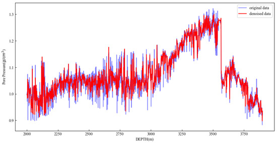
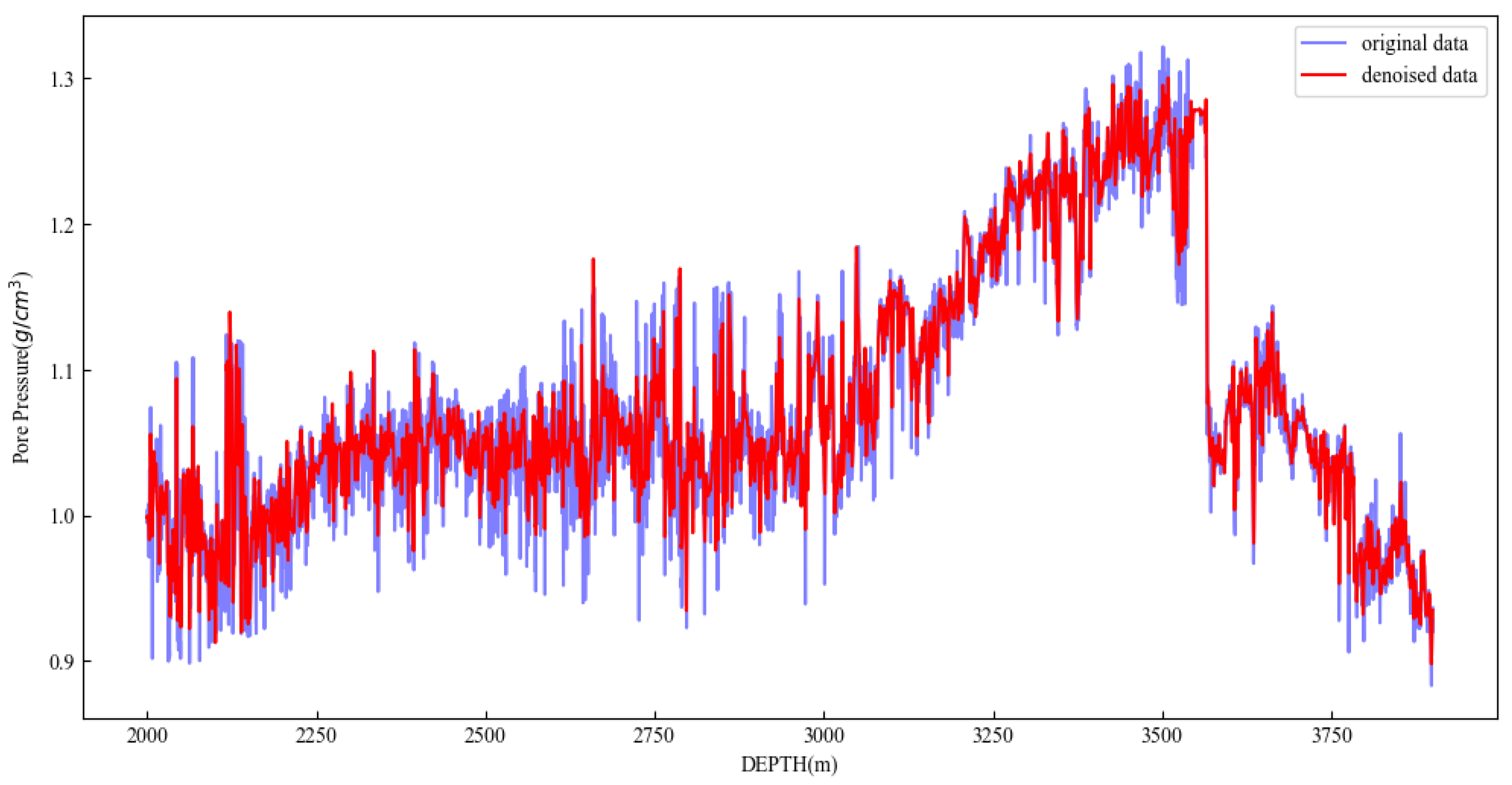
In the formula, denotes the set of coefficients after threshold processing. The advantage of wavelet denoising lies in its ability to adaptively preserve valid signal features based on time-frequency localized analysis, rendering it particularly suitable for processing non-stationary time series. Through the sequential processing of outlier analysis and signal smoothing, this study achieved the cleansing and enhancement of raw data, providing a high-quality data foundation for subsequent modeling. The smoothing effect is shown in Figure 2.
Figure 2.
Example of filtering for noise reduction.
3.3. Label Establishment
Based on the formation mechanism of anomalous formation pressures, formation pressures can be predicted through the response trends of logging curves. When mudstone formations are under-consolidated, their porosity exceeds that of normally consolidated formations, causing logging curves such as acoustic travel time to deviate from the normal consolidation trend line. Such formations are termed anomalously high-pressure formations. Formation pressures can be predicted based on this characteristic.
The Eaton method is currently the most widely employed technique for calculating formation pore pressure in drilling operations, with its computational model presented in Equation (27).
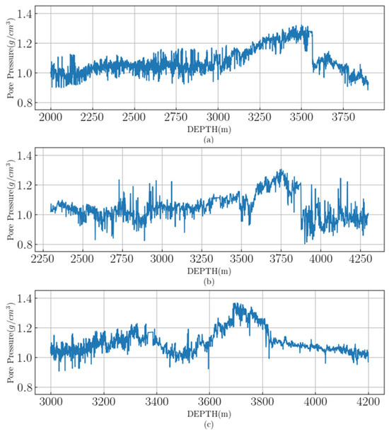
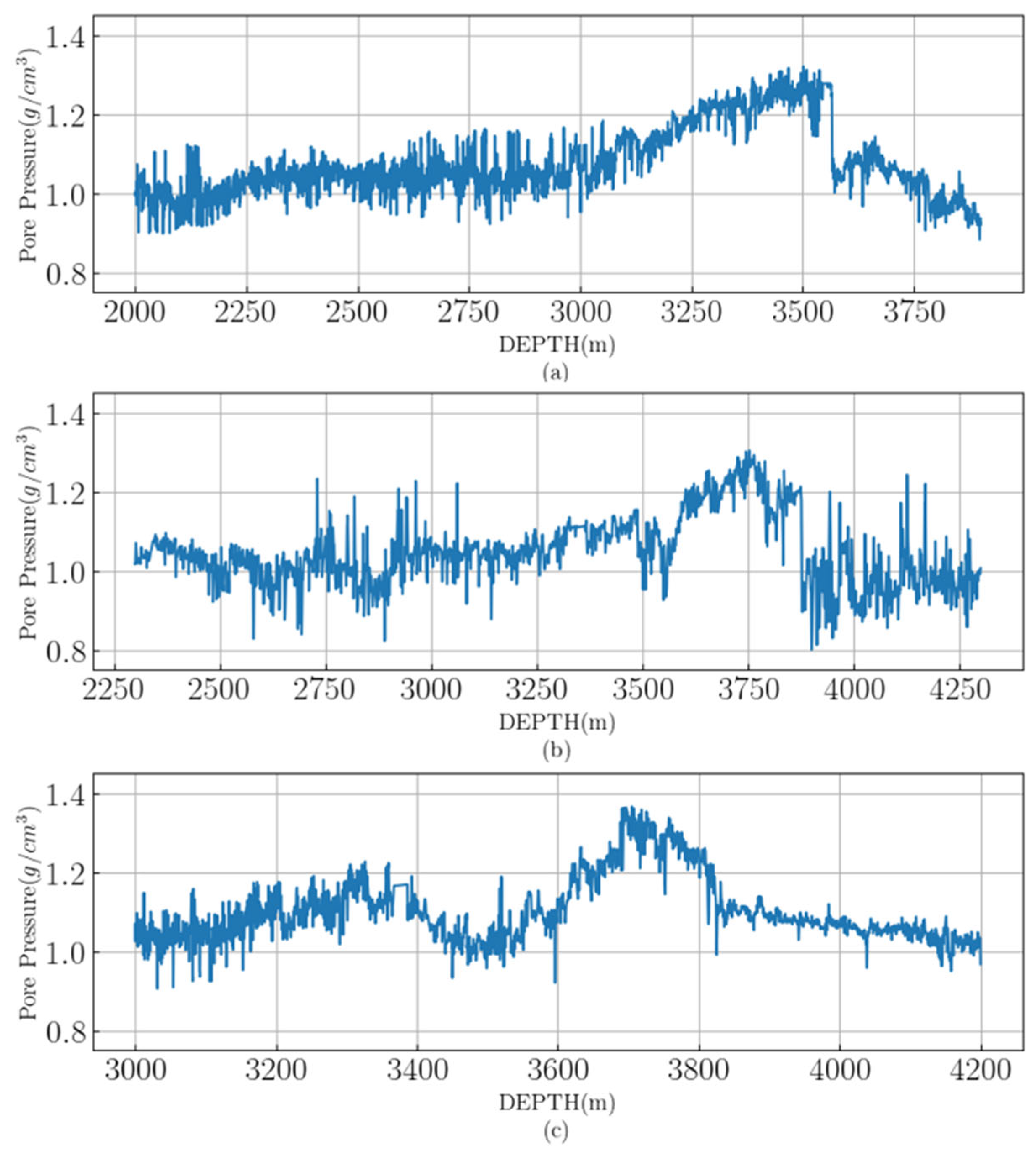
In the equation, denotes the pore pressure gradient, expressed in terms of equivalent drilling fluid density, g/cm3; denotes the overburden pressure gradient, expressed in terms of equivalent drilling fluid density, g/cm3; represents the hydrostatic pressure gradient, expressed in terms of equivalent drilling fluid density, g/cm3; is the logging value at the calculation point; is the parameter value of the normal trend line corresponding to the calculation point; is the Eaton index. This study employs acoustic logging curves (DT24) as the basis for calculating formation pore pressure. The calculated formation pore pressure curves for wells A1, A2, and A3 are presented in Figure 3.
Figure 3.
Calculation results for pore pressure (a) pore pressure of well A1 (b) pore pressure of well A2, (c) pore pressure of well A3.
3.4. Parameter Optimization
Parameter optimization through correlation analysis enables the determination of the degree, direction, and strength of linear relationships between variables, prediction of variable trends, selection of appropriate features, and evaluation of interactions, holding significant theoretical and practical value. This study conducted correlation analysis to identify inter-dependencies among feature variables. The Pearson correlation coefficient was employed, which ranges from −1 to +1. A value of 0 indicates no linear correlation; values greater than 0 signify positive correlation, while values less than 0 indicate negative correlation. The magnitude of the coefficient reflects the strength of the linear relationship.
where represents the correlation coefficient, represents the covariance of variables and , , are the standard deviations of and .
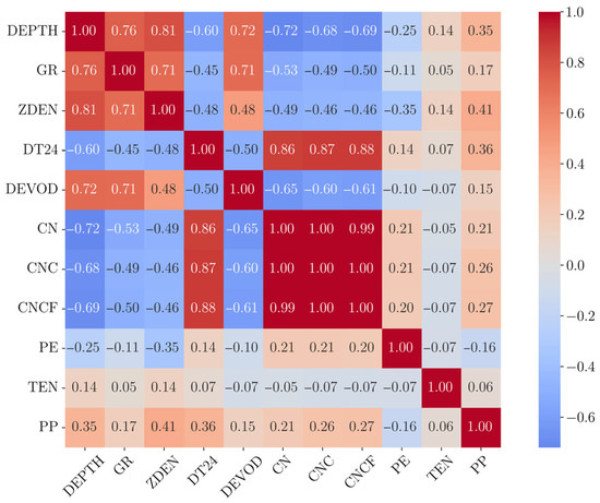
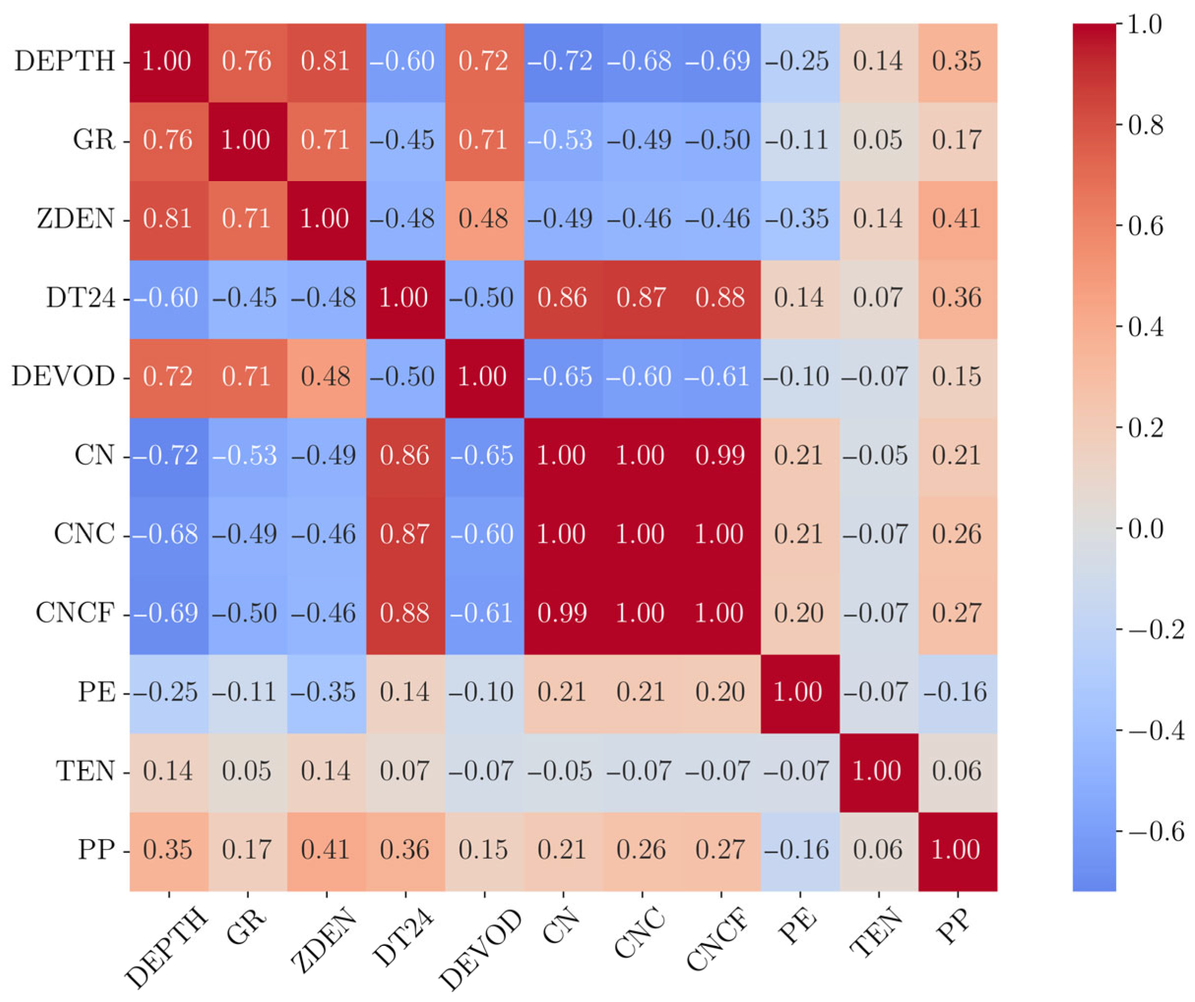
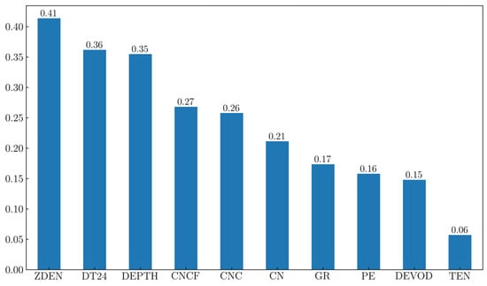
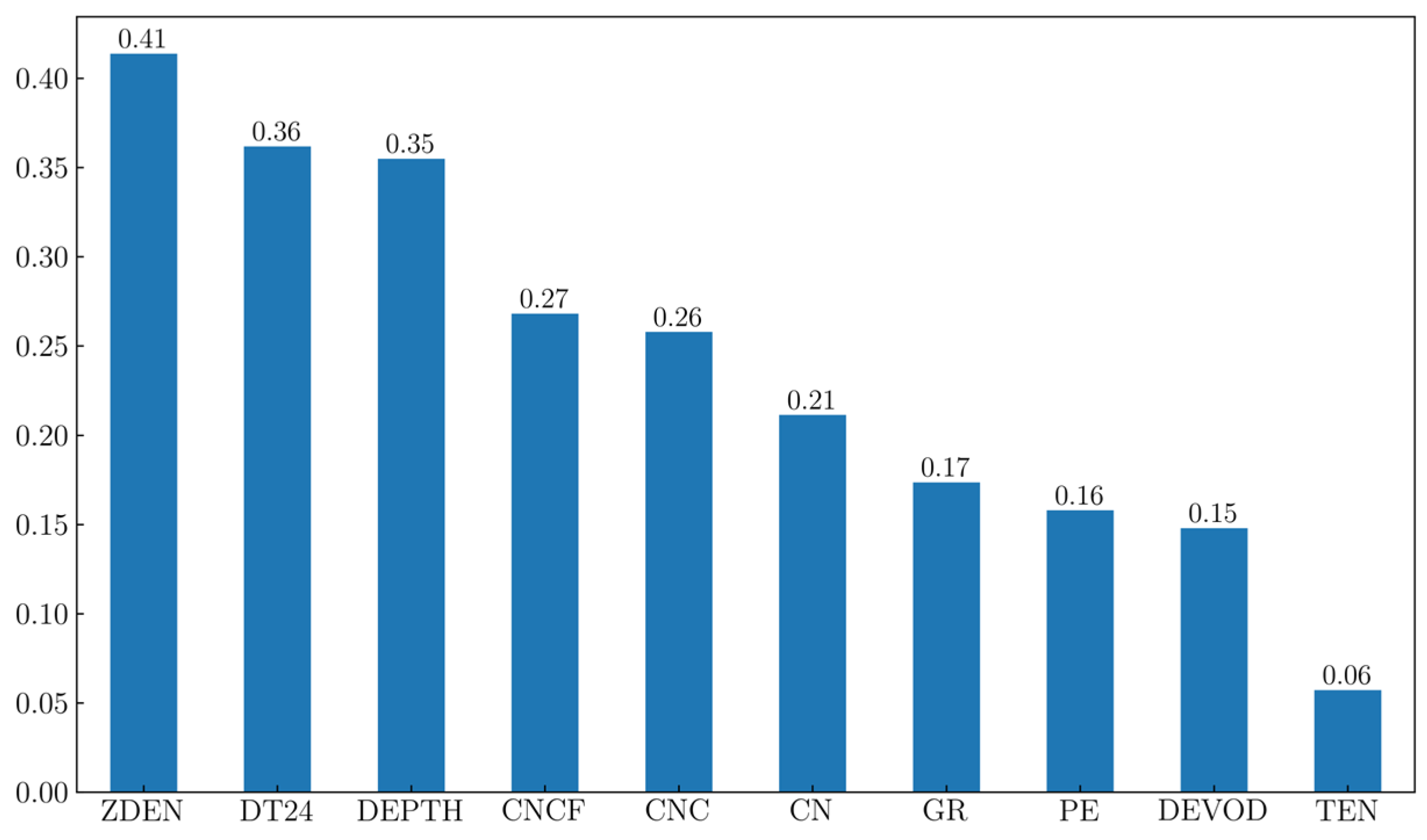
As shown in Figure 4, the heatmap illustrates the correlations between different parameters, with ZDEN, DT24, and CNCF exhibiting relatively high correlations with PP. Figure 5 further corroborates that ZDEN is the parameter most strongly correlated with PP. Although DEPTH shows a certain degree of correlation with PP, it is not suitable as an input parameter for predicting PP due to its significant variation with individual wells and its lack of direct reflection of rock physical properties. CNCF, despite its slightly lower correlation, can still be considered as a predictive indicator. GR, which has a moderate correlation with PP, should also be taken into account because it can reflect the stratigraphic characteristics of the formation. Based on the analysis integrating domain knowledge, expert experience, and multiple feature optimization methods, four parameters were ultimately selected as input features for the intelligent model: density log (ZDEN), acoustic log (DT24), gamma ray log (GR), and corrected compensated neutron log (CNCF). Notably, the mutual information values and correlation coefficients between the kick risk indicator and the three parameters—acoustic log (DT24), density log (ZDEN), and corrected compensated neutron log (CNCF)—ranked highest among all candidate parameters. This finding is highly consistent with field engineering practice and expert experience.
Figure 4.
Parameter correlation heatmap.
Figure 5.
Parameter correlation ranking.
Correlation analysis and sensitivity experiments were employed to optimize the logging parameters, aiming to identify the feature combination most responsive to pore pressure for enhanced model prediction accuracy and generalization capability.
4. Model Establishment
4.1. Evaluation of Metrics for Predictive Models
For regression problems, metrics such as the Root Mean Square Error (RMSE) and Mean Absolute Error (MAE) are typically used to quantify the magnitude of prediction errors, while the coefficient of determination () is used to measure the model’s explanatory power regarding data variance. The definitions of RMSE, MAE, and are as follows:
In the above equations, is the total number of samples, is the true value of the -th sample, is the predicted value for the -th sample, and is the mean of the true values. The standard regression models in this study can be directly evaluated using the metrics defined above. For uncertainty models, the mean of the model’s predicted labels is first calculated and then substituted into the equations for evaluation. Furthermore, performance metrics capable of quantitatively assessing different uncertainty models are required. This study proposes employing Confidence Interval Coverage (CIC) as an evaluation metric. It is calculated by determining the confidence interval for each predicted value and then checking whether the true value falls within that interval. The formula is given in Equation (32):
In the equation, is the indicator function, which equals 1 if the condition is true and 0 otherwise. In the equation, represents the -quantile of the standard normal distribution. For a 95% confidence interval in this study, , . Thus, we can evaluate whether each formation pressure label falls within its confidence interval and thereby assess the coverage rate. The value range of this metric is [0, 1], with values closer to 1 indicating more comprehensive coverage.
4.2. BP and LSTM Models
The study first established formation pressure regression models based on BP (Back propagation Neural Network) and LSTM (Long Short-Term Memory) architectures, using Mean Squared Error (MSE) as the evaluation metric for regression performance. During training, we employed Optuna (1.4.0), an advanced hyper-parameter optimization framework in Python. Optuna automates the search for optimal hyper-parameter combinations by leveraging Python’s conditional statements and loop structures. It supports seamless parallelization of hyper-parameter searches across multiple threads or processes without code modifications. When applied to optimize intelligent algorithms, Optuna’s objective function typically returns the model’s loss or accuracy. In this study, the objective of optimization was to minimize the error in formation pressure regression. The results of the hyper-parameter search are presented in Table 2 [7].
Table 2.
Model parameter optimization results.
4.3. BP and LSTM Models Optimized with Bayesian Layer
Integrating Bayesian layers into feedforward neural networks involves replacing deterministic weights with probability distributions. Specifically, for a weight matrix , as shown in Equation (33), variational parameters are introduced, where the mean is directly parameterized, and the standard deviation is ensured to be positive via the softplus transformation . During forward propagation, sampling is performed using the reparameterization trick.
where denotes element-wise multiplication, and is random noise from a standard normal distribution.
This design enables gradient backpropagation via Monte Carlo estimation, allowing optimization of variational parameters. For a Bayesian feedforward network with hidden layers, the forward propagation process is formulated as Equation (34).
where is the activation of the -th layer, is the activation function, and , are weights and biases sampled from their respective distributions. The output layer produces predictive means, while the model learns homoscedastic observation noise .
The loss function during training comprises the negative log-likelihood and a KL divergence term as Equation (35).
Under the Gaussian likelihood assumption, the negative log-likelihood term expands to Equation (36)
where is the neural network output, and is the observation noise standard deviation.
During prediction, the predictive distribution is approximated via multiple sampling as Equation (37).
The predictive mean Equation (38) and variance Equation (39) are estimated as sample statistics.
In the equation, stands the number of samples. The first term in the variance represents epistemic uncertainty, while the second term captures aleatoric uncertainty. For time series modeling, Long Short-Term Memory (LSTM) networks capture long-term dependencies through gating mechanisms. Combining Bayesian layers with LSTM retains sequential modeling capabilities while quantifying predictive uncertainty. The proposed architecture adopts a hierarchical design: the LSTM layer extracts temporal features, and the Bayesian probabilistic layer handles uncertainty quantification.
Given an input sequence , the LSTM computes hidden states via the following gating mechanisms as Equation (40)
where represent input, forget, and output gates, is the candidate cell state, is the cell state, is the hidden state; and is the sigmoid activation function.
The hidden state at the final time step serves as the sequence representation and is fed into the Bayesian probabilistic layer (implemented as a Dense Variational layer for uncertainty modeling. Its forward propagation is shown in Equation (41).
In the equation, and represent the weights and biases sampled from the variational posterior distribution.
As shown in Equation (42), The training objective remains ELBO maximization, but the KL divergence weight is set to for adaptive regularization.
This configuration ensures strong regularization on small datasets while reducing prior constraints on large datasets.
During prediction, multiple forward passes generate predictive samples in Equation (43), and the predictive mean and variance are computed similarly to the feedforward network, shown in Equations (44) and (45).
4.4. BP and LSTM Models with MC Dropout Layer Applied
Integrating MC Dropout into feedforward neural networks involves inserting Dropout layers between hidden layers of a traditional architecture. For a deep network with hidden layers, the forward propagation process is formulated as Equation (46).
where is the activation function, and is the dropout mask vector (with elements drawn from a Bernoulli distribution) that remains fixed during both training and testing phases. During training, the loss function combines a standard supervised learning objective (e.g., mean squared error or cross-entropy) with weight decay regularization as shown in Equation (47).
Here, is the task-specific loss, and is the regularization coefficient. Note that the regularization effect of MC Dropout is implicitly embedded in the dropout operation itself; thus, is typically set to a small value.
During prediction, stochastic forward passes with dropout enabled generate a set of predictive samples . The predictive means and variance are computed as Equations (48) and (49).
For LSTM networks, MC Dropout is applied to the linear transformations preceding the three gating mechanisms: input gate, forget gate, and output gate. The implementation details are shown in Equation (50).
where is the input gate activation, and are the dropout mask applied to hidden states and inputs.
To ensure temporal consistency, the same dropout mask is retained across all time steps of a sequence. This design stabilizes uncertainty propagation along the time dimension.
During prediction, for an input sequence , multiple stochastic forward passes yield the predictive distribution. The final prediction and its uncertainty are estimated as Equations (51) and (52).
where denotes the LSTM output under the -th dropout mask.
4.5. Risk Assessment Method Based on Probability Density
The safety factor in drilling mud density design refers to an additional margin added to the formation pore pressure equivalent density to ensure wellbore stability and prevent well control incidents such as kicks, wellbore collapse, or differential sticking. Key constraints include: the minimum density limit to prevent kicks, the minimum density to prevent wellbore collapse, the maximum density to avoid differential sticking, and the maximum density to prevent fluid loss.
As this study focuses on kick risk, the uncertainty expression for the minimum drilling mud density limit to prevent kicks is defined by Equation (53), where is the swab pressure safety factor (set to 0.05 in this study), is the pore pressure equivalent density, and is the differential sticking safety factor (set to 0.10 for target blocks with high-pressure gas).
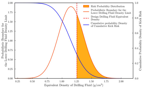
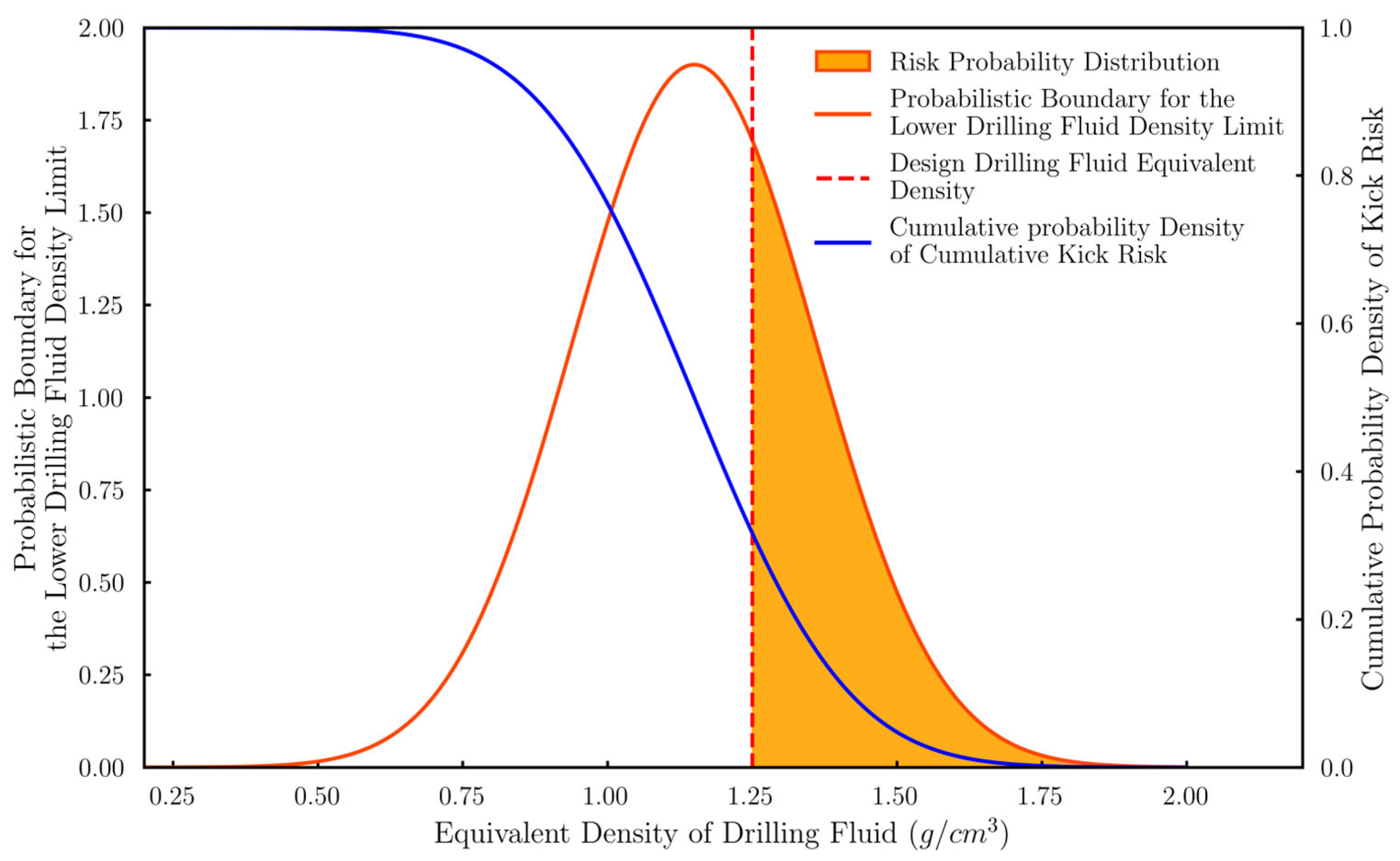
Following Zhou et al. [20] the probabilistic boundary of the minimum mud density to prevent kicks is derived by combining uncertain pore pressure predictions with safety factors. As shown in Figure 6, the risk probability distribution is represented as a confidence interval, and the cumulative kick risk is computed as the cumulative probability density of the designed mud density value within this interval. Since a decrease in mud density increases the cumulative kick risk, the probability density curve accumulates from higher to lower mud densities, as shown in Equation (54), in which is design drilling fluid equivalent density, is cumulative probability density of cumulative kick risk.
Figure 6.
Principle of probability density risk assessment method.
5. Results and Discussions
5.1. Comparing Uncertainty Methods with Deterministic Models
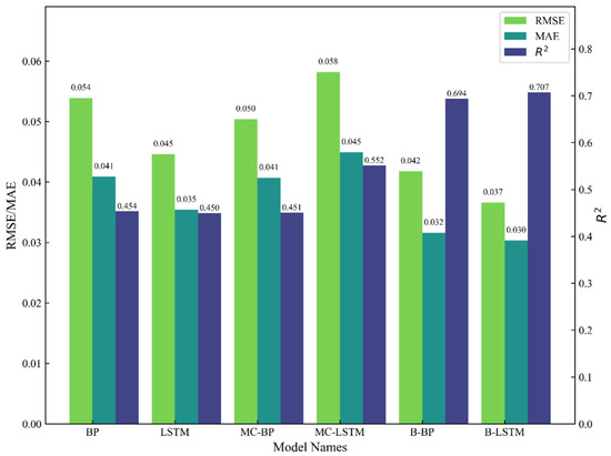
We first compared the basic regression accuracy of foundational BP and LSTM models against their counterparts enhanced with MC Dropout (MC-BP, MC-LSTM) and Bayesian layers (B-BP, B-LSTM). Performance was validated using the MAE, RMSE, and R2 metrics defined in Equations (29)–(31).
As shown in Figure 7, the baseline BP and LSTM models exhibited lower R2 values (approximately 0.450 to 0.552) and higher RMSE, reflecting their limited fitting capability due to the specific complexity of formation pressure fluctuations. In contrast, models incorporating optimized weight layers demonstrated significant improvement across multiple metrics. Specifically, the MC-LSTM model with MC Dropout achieved a lower RMSE of about 0.041, while the B-LSTM model attained a similar level. This indicates that these optimization methods effectively reduce prediction errors. Regarding the metric, the B-LSTM and B-BP models performed notably well, with values reaching approximately 0.667 and 0.552, respectively, surpassing the baseline models. This highlights the potential of Bayesian methods in enhancing model robustness and explanatory variance.
Figure 7.
Model testing results.
All models exhibited relatively balanced performance in RMSE and MAE metrics, with RMSE values ranging from approximately 0.037 to 0.058 and MAE values between 0.030 and 0.045. Models using MC Dropout showed no substantial improvement in MAE and RMSE compared to the baseline models. This is expected, as MC Dropout does not directly alter the target model’s architecture but rather quantifies uncertainty in its predictions. In contrast, Bayesian layers can optimize the model’s weight structure through backpropagation, thereby refining regression results within a certain range. Consequently, their RMSE and MAE metrics are comparatively more favorable.
5.2. Comparative Advantages Among Uncertainty Methods
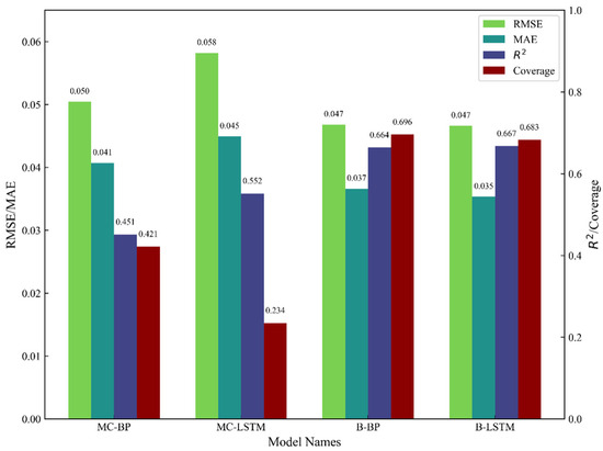
As previously outlined, we introduced two methods for quantifying model uncertainty: MC Dropout and Bayesian layer optimization via Bayes by Backprop, applying both to BP and LSTM models. By employing the Confidence Interval Coverage (CIC) metric defined in Section 4.1 (Equation (32)), we can intuitively compare the coverage of uncertainty estimates provided by each model. Experimental results reveal a pronounced performance gap between the two optimization strategies. As shown in Figure 8, the two models utilizing MC Dropout—MC-BP and MC-LSTM—achieved CIC values of only 0.421 and 0.234, respectively. This outcome falls below the desired level, indicating that the confidence intervals estimated by this method are too narrow and fail to adequately encompass data variability, leading to an underestimation of uncertainty.
Figure 8.
Comparison of uncertainty model performance.
In contrast, models optimized with Bayes by Backprop demonstrated stronger calibration capability. The B-BP model achieved a CIC of 0.696, and the B-LSTM model reached 0.683. This comparison clearly reveals that, regardless of whether the base predictor is BP or LSTM, the Bayes by Backprop method—by introducing probability distributions over weight parameters—systematically yields more reliable and wider confidence intervals. Therefore, it can be concluded that for enhancing the reliability of model uncertainty quantification, the Bayes by Backprop optimization strategy is superior to the MC Dropout method, providing a more solid theoretical foundation and practical efficacy for generating accurate probabilistic predictions.
5.3. Engineering Application
The model predictions enable the establishment of pore pressure uncertainty assessment results for the target well section. Following the risk assessment method based on probability density interference established in Section 4.5, the interference risk probability can be calculated by incorporating the designed drilling mud density. This study utilizes the designed mud density from the drilling plan for Well A3 (as shown in Table 3) as the interference condition for the calculation.
Table 3.
Designed drilling mud density for Well A3.
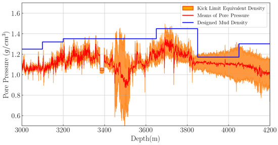
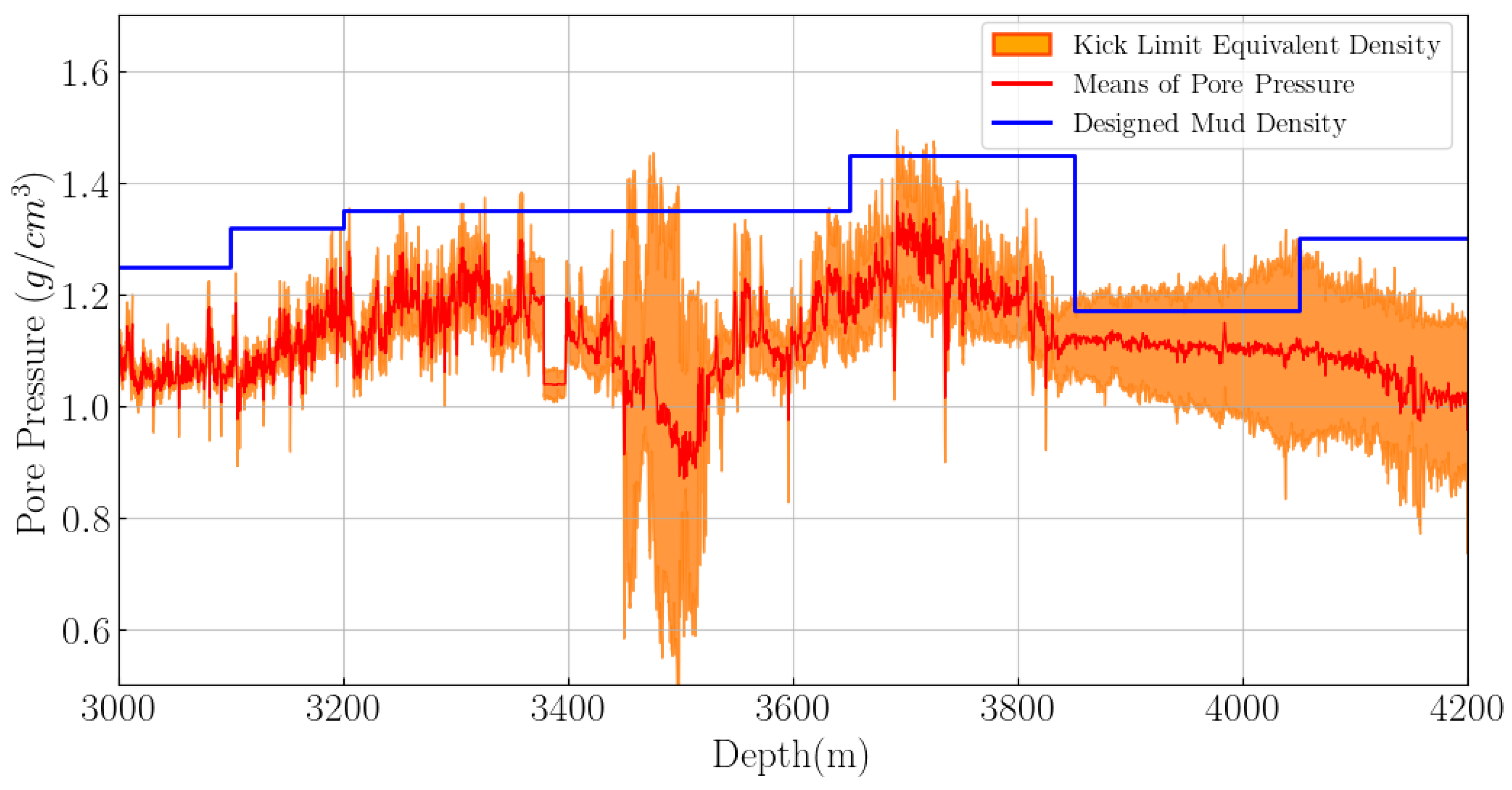
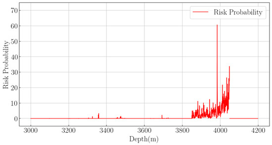
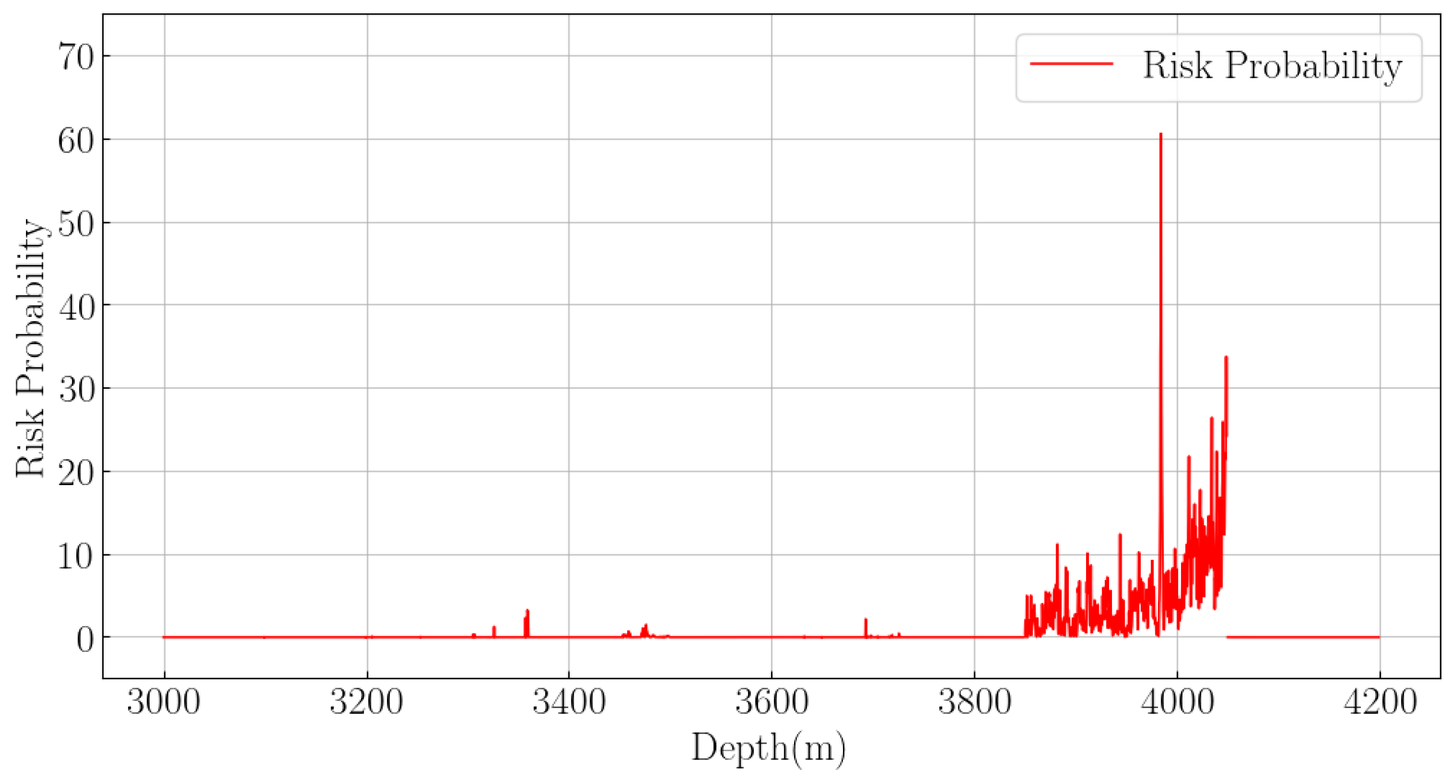
The overlap and interference between the pore pressure confidence interval and the designed mud density are illustrated in Figure 9. The interference risk value for this well section can be obtained through integration, and its distribution curve along the well depth is shown in Figure 10.
Figure 9.
Pore pressure confidence interval and drilling fluid design density overlap results.
Figure 10.
Well section interference risk value curve.
From this result, the cumulative risk probability density for the well can be integrated. The results indicate higher risk at depths of 3983 m and 4048 m. Referring to the well history in Table 1, a kick precursor was recorded at 4050 m in this well. This confirms that the proposed method, through risk uncertainty assessment, accurately identifies potential kick risks, providing valuable reference for drilling design.
For decision-making in drilling design, we recommend implementing tiered thresholds based on the risk probability value to aid risk management. When the risk probability exceeds 30%, it serves as a medium-risk threshold, indicating a need for enhanced monitoring or adjustment of drilling parameters (such as optimizing ECD control). A value exceeding 50% constitutes a high-risk threshold, suggesting a significant kick risk that warrants proactive optimization of the drilling fluid density or revision of the wellbore structure.
The risk assessment methodology proposed in this study provides value not only in post hoc validation of drilling events but, more significantly, offers a forward-looking and quantifiable basis for decision-making in drilling engineering. By utilizing actual measurement data from existing wells, an uncertainty evaluation model for pore pressure can be established. This model can be spatially extrapolated to prospective well locations to predict the probabilistic distribution of formation pressure, thereby furnishing a theoretical foundation for optimizing drilling fluid density design. As illustrated in Figure 9, comparing the relationships among the designed drilling fluid density, the mean pore pressure, and the equivalent density for kick tolerance elucidates the dynamic characteristics of the safe drilling fluid window with depth. This analysis guides engineers to appropriately increase the mud weight or meticulously manage the Equivalent Circulating Density (ECD) in critical zones, achieving an optimal balance between well control safety and formation integrity. Furthermore, the methodology allows for various inputs—such as drilling fluid density, wellbore structure, and operational parameters—to rapidly generate and compare risk probability profiles for different design scenarios. This facilitates a quantitative safety evaluation of multiple alternatives during the design phase, promoting a shift in drilling design from reliance on empirical judgment to decisions grounded in quantitative risk assessment. Consequently, it provides a scientific basis for selecting engineering solutions with lower risk and higher operational feasibility.
6. Conclusions
This study innovatively proposes a two-stage pre-drilling kick risk assessment methodology based on a Bayesian Long Short-Term Memory (BLSTM) network. The systematic workflow integrates “pore pressure uncertainty prediction” with “distribution interference analysis” to achieve probabilistic quantification of drilling risks. The research demonstrates that the Bayes by Backprop optimization strategy significantly enhances uncertainty characterization. The B-LSTM model achieved a mean absolute error of 0.037 and a confidence interval coverage rate of 69.6% in the test well section, representing a 26.7% improvement in prediction accuracy over the traditional LSTM model. Risk assessment based on the distribution interference criterion successfully identified a 60% kick risk probability in the 3893–4048 m section of Well A3, which closely aligned with the actual kick incident recorded during drilling. This methodology provides a novel risk assessment paradigm for drilling engineering that combines physical interpretability with statistical reliability, offering significant practical value for safety decision-making in complex formations. Future work could focus on multi-source data integration and real-time dynamic risk assessment.
Author Contributions
Conceptualization, B.X., C.Z. and D.Z.; methodology, C.Z. and D.Z.; software, G.S. and C.Z.; validation, G.S., H.X. and H.L.; formal analysis, G.S. and C.Z.; investigation, H.X. and H.L.; resources, B.X. and G.S.; data colouration, H.X. and H.L.; writing—original draft preparation, C.Z. and D.Z.; writing—review and editing, B.X., G.S. and Z.Z.; visualization, C.Z. and H.L.; supervision, B.X., G.S. and Z.Z.; project administration, B.X., G.S. and Z.Z. All authors have read and agreed to the published version of the manuscript.
Funding
This research received no external funding.
Data Availability Statement
The data are not publicly available due to involve the information of Chinese oil fields and need to be kept confidential.
Conflicts of Interest
Author Boyi Xia was employed by the Greatwall Drilling Engineering Research Institute, authors Gang Sun, Hongyu Xie and Haining Liu were employed by the PetroChina (Beijing) Digital Intelligent Research Institute Co., Ltd. The remaining authors declare that the research was conducted in the absence of any commercial or financial relationships that could be construed as a potential conflict of interest.
References
- Rashidi, M.; Asadi, A. An Artificial Intelligence Approach in Estimation of Formation Pore Pressure by Critical Drilling Data. In Proceedings of the 52nd U.S. Rock Mechanics/Geomechanics Symposium, Seattle, WA, USA, 17–20 June 2018. [Google Scholar]
- Abdulmalek, A.S.; Elkatatny, S.; Abdulraheem, A.; Mahmoud, M.; Abdulwahab, Z.A.; Mohamed, I.M. Pore Pressure Prediction While Drilling Using Fuzzy Logic. In Proceedings of the SPE Kingdom of Saudi Arabia Annual Technical Symposium and Exhibition, Dammam, Saudi Arabia, 23–26 April 2018. [Google Scholar]
- Hadi, F.; Eckert, A.; Almahdawi, F. Real-Time Pore Pressure Prediction in Depleted Reservoirs Using Regression Analysis and Artificial Neural Networks. In Proceedings of the SPE Middle East Oil and Gas Show and Conference, Manama, Bahrain, 18 March 2019; p. D031S034R002. [Google Scholar]
- Sun, B.; Cheng, Y.; Han, Z.; Yan, C.; Yang, J. Experimental study of a multimechanism formation pressure prediction model influenced by shale content. Geoenergy Sci. Eng. 2024, 233, 212486. [Google Scholar] [CrossRef] [Scilit]
- Cao, S.; Wang, C.; Niu, Q.; Zheng, Q.; Shen, G.; Chen, B.; Shi, X.; Zhang, W. Enhancing pore pressure prediction accuracy: A knowledge-driven approach with temporal fusion transformer. Geoenergy Sci. Eng. 2024, 238, 212839. [Google Scholar] [CrossRef] [Scilit]
- Zhang, Q.; Yan, Z.; Fan, X.; Li, Z.; Zhao, P.; Shuai, J.; Jia, L.; Liu, L. Field Monitoring and Identification Method for Overflow of Fractured-Vuggy Carbonate Reservoir. Energies 2023, 16, 2399. [Google Scholar] [CrossRef] [Scilit]
- Wu, L.; Zhou, D.; Li, G.; Gong, N.; Song, X.; Zhang, Q.; Yan, Z.; Pan, T.; Zhang, Z. Kick Risk Diagnosis Method Based on Ensemble Learning Models. Processes 2024, 12, 2704. [Google Scholar] [CrossRef] [Scilit]
- Whittaker, J.A.; Rekab, K.; Thomason, M.G. A Markov chain model for predicting the reliability of multi-build software. Inf. Softw. Technol. 2000, 42, 889–894. [Google Scholar] [CrossRef] [Scilit]
- Langseth, H.; Portinale, L. Bayesian networks in reliability. Reliab. Eng. Syst. Safe. 2007, 92, 92–108. [Google Scholar] [CrossRef] [Scilit]
- Cai, B.; Liu, Y.; Zhang, Y.; Fan, Q.; Yu, S. Dynamic Bayesian networks based performance evaluation of subsea blowout preventers in presence of imperfect repair. Expert Syst. Appl. 2013, 40, 7544–7554. [Google Scholar] [CrossRef] [Scilit]
- Wu, S.; Zhang, L.; Zheng, W.; Liu, Y.; Lundteigen, M.A. A DBN-based risk assessment model for prediction and diagnosis of offshore drilling incidents. J. Nat. Gas Sci. Eng. 2016, 34, 139–158. [Google Scholar] [CrossRef] [Scilit]
- Shi, J. Dynamic Risk Assessment and Accident Early Warning for Natural Gas Hydrate Encountered by Deepwater Drillin. Master’s Thesis, China University of Petroleum, Beijing, China, 2019. [Google Scholar]
- Guan, Z.; Sheng, Y. Quantitative characterization of ECD uncertainty based on uncertainty theory. Drill. Fluids Complet. Fluids 2018, 35, 62–67. [Google Scholar]
- Sheng, Y. Research on Drilling Engineering Risk Assessment and Control Technology. Ph.D. Thesis, China University of Petroleum (East China), Qingdao, China, 2019. [Google Scholar]
- Xu, Y.; Liu, K.; He, B.; Pinyaeva, T.; Li, B.; Wang, Y.; Nie, J.; Yang, L.; Li, F. Risk pre-assessment method for regional drilling engineering based on deep learning and multi-source data. Petrol. Sci. 2023, 20, 3654–3672. [Google Scholar] [CrossRef] [Scilit]
- Gal, Y.; Ghahramani, Z. Dropout as a Bayesian Approximation: Representing Model Uncertainty in Deep Learning. arXiv 2015, arXiv:1506.02142. [Google Scholar] [CrossRef] [Scilit]
- Shamsi, A.; Asgharnezhad, H.; Abdar, M.; Tajally, A.; Khosravi, A.; Nahavandi, S.; Leung, H. Improving mc-dropout uncertainty estimates with calibration error-based optimization. arXiv 2021, arXiv:2110.03260. [Google Scholar]
- Olivier, A.; Shields, M.D.; Graham-Brady, L. Bayesian neural networks for uncertainty quantification in data-driven materials modeling. Comput. Methods Appl. Mech. Eng. 2021, 386, 114079. [Google Scholar] [CrossRef] [Scilit]
- Blundell, C.; Cornebise, J.; Kavukcuoglu, K.; Wierstra, D. Weight Uncertainty in Neural Networks. arXiv 2015, arXiv:1505.05424. [Google Scholar] [CrossRef] [Scilit]
- Zhou, D.; Zhu, Z.; Zhou, C.; Song, X.; Li, G.; Zhang, C.; Li, Q.; Li, S. Unsupervised Learning—Based Kick Risk Warning with Dynamic Thresholds and Knowledge Embedding. SPE J. 2025, 30, 6584–6602. [Google Scholar] [CrossRef] [Scilit]

Disclaimer/Publisher’s Note: The statements, opinions and data contained in all publications are solely those of the individual author(s) and contributor(s) and not of MDPI and/or the editor(s). MDPI and/or the editor(s) disclaim responsibility for any injury to people or property resulting from any ideas, methods, instructions or products referred to in the content. |
© 2026 by the authors. Licensee MDPI, Basel, Switzerland. This article is an open access article distributed under the terms and conditions of the Creative Commons Attribution (CC BY) license.