


Abstract
Accurate State-of-Health (SOH) estimation for second-life batteries is a critical challenge due to unavailable first-life historical data. This work introduces the Prior-Informed Hierarchical Fusion Network (PI-HFN), a flexible deep learning framework to address this information asymmetry. The model leverages a historical degradation vector from the battery’s first life as a prior condition to guide the interpretation of its current electrochemical state. This prior-conditioning is achieved by initializing a recurrent neural network, which processes instantaneous second-life data, with the historical information. The framework’s efficacy was validated across two comprehensive case studies. In Case Study 1 on NMC cells using multimodal EIS and DCIR inputs, the PI-HFN achieved a state-of-the-art average RMSE of 1.91%. Case Study 2 on a large-scale LFP dataset, using only DCIR inputs, further demonstrated the framework’s robustness and flexibility. Both studies confirmed through systematic ablation studies that the historical prior (BFN) and the hierarchical fusion strategy (PFN) are crucial for high accuracy, with the historical prior proving to be the dominant factor in mitigating errors in data-sparse SOH regions. The model also shows excellent deployment potential, with an inference latency of 15.8 ms on an RK3568 edge platform after INT8 quantization. This study validates that conditioning deep learning models with historical priors offers a robust, flexible, and practical pathway for evaluating second-life batteries, supporting their integration into the circular economy.
1. Introduction
Driven by the strategic transformation of the global energy structure towards sustainability, lithium-ion batteries (LIBs) have become an indispensable core technology in key areas such as electric vehicles and large-scale grid energy storage due to their advantages of high energy density and long cycle life [1]. As a control unit that ensures the safe and efficient operation of the battery pack, the accuracy of the battery management system (BMS) directly determines the performance and reliability of the entire system. Among the many key tasks of the BMS, the real-time and accurate estimation of the battery state of health (SOH) constitutes the most basic and challenging link. SOH not only quantifies the degree of performance degradation of the battery due to cycling and calendar aging [2], but is also a key input parameter for predicting its remaining useful life, formulating optimized operation strategies, and preventing catastrophic thermal runaway events [3].
Currently, the system of SOH estimation methods has developed quite large and can be roughly divided into three technical routes: direct measurement method, model method and data-driven method [4]. Although direct measurement methods such as ampere-hour integration are intuitive in principle, they face severe challenges in practical applications: their estimation results are highly dependent on the accurate prediction of the initial capacity, and in long-term operation, the inherent drift and measurement noise of the current sensor will continue to accumulate, causing the estimation error to diverge over time [5]. Model methods are committed to characterizing the electrochemical dynamics inside the battery by constructing complex electrochemical models or equivalent circuit models, and then inferring its health status. Although such methods can achieve high fidelity in theory [6], their application faces a double dilemma: first, the model itself has high computational complexity and places high demands on the hardware resources of the BMS; second, the model parameters, such as resistance and capacitance are themselves functions of the aging state and will continue to evolve with the battery life cycle. The online identification process of the parameters is not only algorithmically complex, but also usually requires specific current excitation conditions, which greatly limits their actual deployment and application under dynamically changing conditions [7].
In recent years, data-driven methods have attracted much attention because they can bypass the precise description of complex electrochemical mechanisms. This type of method directly learns from massive amounts of measurement data and constructs a nonlinear mapping relationship between SOH and external measurable features [8]. Among the many available input features, information derived from electrochemical measurements has proven particularly effective. Electrochemical impedance spectroscopy (EIS), a powerful nondestructive in situ detection technique, can provide multidimensional and in-depth information about the internal state of the battery [9]. Different frequency regions of its Nyquist plot correspond to different electrochemical processes: the real axis intercept in the high-frequency region reflects the combined ohmic internal resistance of the electrolyte, separator, and electrode materials; the semicircle in the mid-frequency region is closely related to the charge transfer process at the electrode/electrolyte interface and the characteristics of the solid electrolyte interface; and the oblique line in the low-frequency region characterizes the diffusion dynamics of lithium ions in the solid-phase active material. Therefore, features extracted from EIS, such as the charge transfer resistance, which directly reflects the core mechanism of interface aging, have been widely confirmed to have a strong monotonic correlation with capacity decay [10]. Meanwhile, the DC internal resistance (DCIR) measured by standard pulse testing, although its information dimension is lower than that of EIS, has become a widely used and concise degradation indicator to characterize the decline of battery power characteristics due to its simple measurement process and easy integration in BMS [11].
In recent years, data-driven methods have attracted much attention because they can bypass the precise description of complex electrochemical mechanisms. This type of method directly learns from massive amounts of measurement data and constructs a nonlinear mapping relationship between SOH and external measurable features [8]. Recently, advanced deep learning architectures, particularly Transformers, have emerged as powerful tools for capturing long-term dependencies in battery aging data. For instance, Chen et al. [9] proposed a hybrid framework integrating LSTM and Transformer networks, utilizing multi-head self-attention to capture global degradation dependencies for accurate SOH estimation. Similarly, Antony et al. [10] developed a Transformer-enhanced multi-modal sensing approach combined with Convolutional Autoencoders, demonstrating superior performance in fault detection and risk management. While these sequence-based models have achieved remarkable accuracy, among the many available input features, information derived from electrochemical measurements has proven particularly effective. Electrochemical impedance spectroscopy (EIS), a powerful nondestructive in situ detection technique, can provide multidimensional and in-depth information about the internal state of the battery [11]. Different frequency regions of its Nyquist plot correspond to different electrochemical processes: the real axis intercept in the high-frequency region reflects the combined ohmic internal resistance of the electrolyte, separator, and electrode materials; the semicircle in the mid-frequency region is closely related to the charge transfer process at the electrode/electrolyte interface and the characteristics of the solid electrolyte interface; and the oblique line in the low-frequency region characterizes the diffusion dynamics of lithium ions in the solid-phase active material. Therefore, features extracted from EIS, such as the charge transfer resistance, which directly reflects the core mechanism of interface aging, have been widely confirmed to have a strong monotonic correlation with capacity decay [12]. Meanwhile, the DC internal resistance (DCIR) measured by standard pulse testing, although its information dimension is lower than that of EIS, has become a widely used and concise degradation indicator to characterize the decline of battery power characteristics due to its simple measurement process and easy integration in BMS [13].
However, a critical research gap remains, as the vast majority of published studies are based on an idealized premise: the availability of complete and continuous historical data from the beginning of battery life (BOL). This model breaks down when applied to secondary lithium-ion batteries (SLBs), which are crucial for a circular economy [14]. For these retired batteries, key prior information from their initial use (e.g., initial capacity and accumulated cycle history) is often unavailable or unreliable due to inconsistent data recording and proprietary barriers. This “information asymmetry” constitutes a major technical bottleneck, specifically, this asymmetry refers to the unavailability of high-granularity raw time-series data due to storage and privacy constraints. However, with the implementation of traceability standards like the Battery Passport, accessing low-dimensional summary statistics is becoming increasingly feasible. Current approaches to this problem include: ref. [15] using random forests to estimate SOH based on electrical and temperature signals from the first few seconds of operation, ignoring relevant information from prior use; ref. [16] generating degradation trajectories using porous electrode theory and employing PINN to estimate current SOH, which requires significant computational resources; and ref. [17] processing EIS data with a multilayer perceptron, which has limited model capacity. These methods generally assume that the aging trajectory during initial use is unavailable. However, with the increasing maturity of the battery recycling industry and stricter traceability requirements, obtaining charging/discharging data or partial charging/discharging characteristics from the initial use is becoming increasingly feasible [18]. To address this pressing challenge, this study proposes a framework designed to effectively leverage the limited historical summary data available from a battery’s first life. The core hypothesis is that by using this historical trajectory as a prior condition to interpret the battery’s current electrochemical state, characterized by EIS and DCIR, a more accurate and robust SOH estimation for SLBs can be achieved.
To verify this hypothesis, we systematically designed three scenarios to simulate different levels of real-world information completeness to explore the feasibility and accuracy of SOH estimation: (1) an ideal benchmark scenario with complete information; (2) a scenario with unknown initial capacity but known cycle history; and (3) a scenario with completely unknown initial capacity and cycle history—a scenario that realistically reproduces the “blind test” challenge faced in secondary battery recycling and screening. Through this work, this paper aims to provide a practical, low-cost, and reliable methodology for evaluating the health status and remaining application value of secondary batteries, thereby providing key technical support for building a safe and efficient battery cascade utilization industry chain.
2. Methodology
2.1. Overall Framework: A Prior-Informed Hierarchical Fusion Network
To accurately estimate the state-of-health of second-life batteries, this study constructs a deep learning model specifically designed to fuse historical information from the battery’s first life with its present electrochemical measurements. The proposed model is termed the Prior-Informed Hierarchical Fusion Network (PI-HFN). The design philosophy of this network is predicated on a central hypothesis: a battery’s historical degradation trajectory does not constitute a set of features independent of its current state, but rather acts as a prior condition that profoundly influences and shapes its present electrochemical behavior. Therefore, the PI-HFN, through its hierarchical structure, aims to explicitly model this intrinsic conditional dependency between historical information and current measurement data, rather than employing a simple parallel-processing approach.
The overall objective of the model is to learn a non-linear mapping function f to estimate the SOH from three heterogeneous input sources, such that . Here, represents the currently measured electrochemical impedance spectrum, denotes the dynamic resistance sequence measured at key voltage points, and is the abstract vector summarizing the battery’s historical degradation trajectory from its first life-cycle. To achieve this, the PI-HFN architecture comprises three synergistic core modules: a prior encoder for processing the historical degradation trajectory, a parallel state encoder for extracting the instantaneous electrochemical information, and a decoder for the final SOH regression.
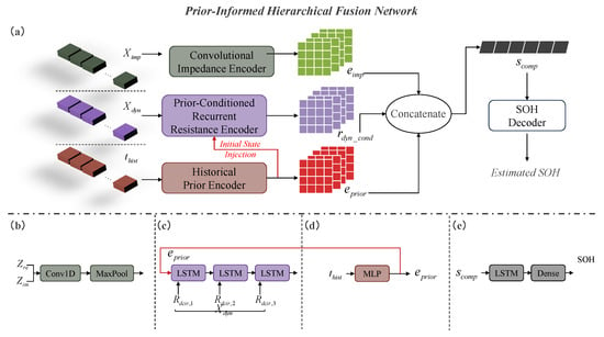
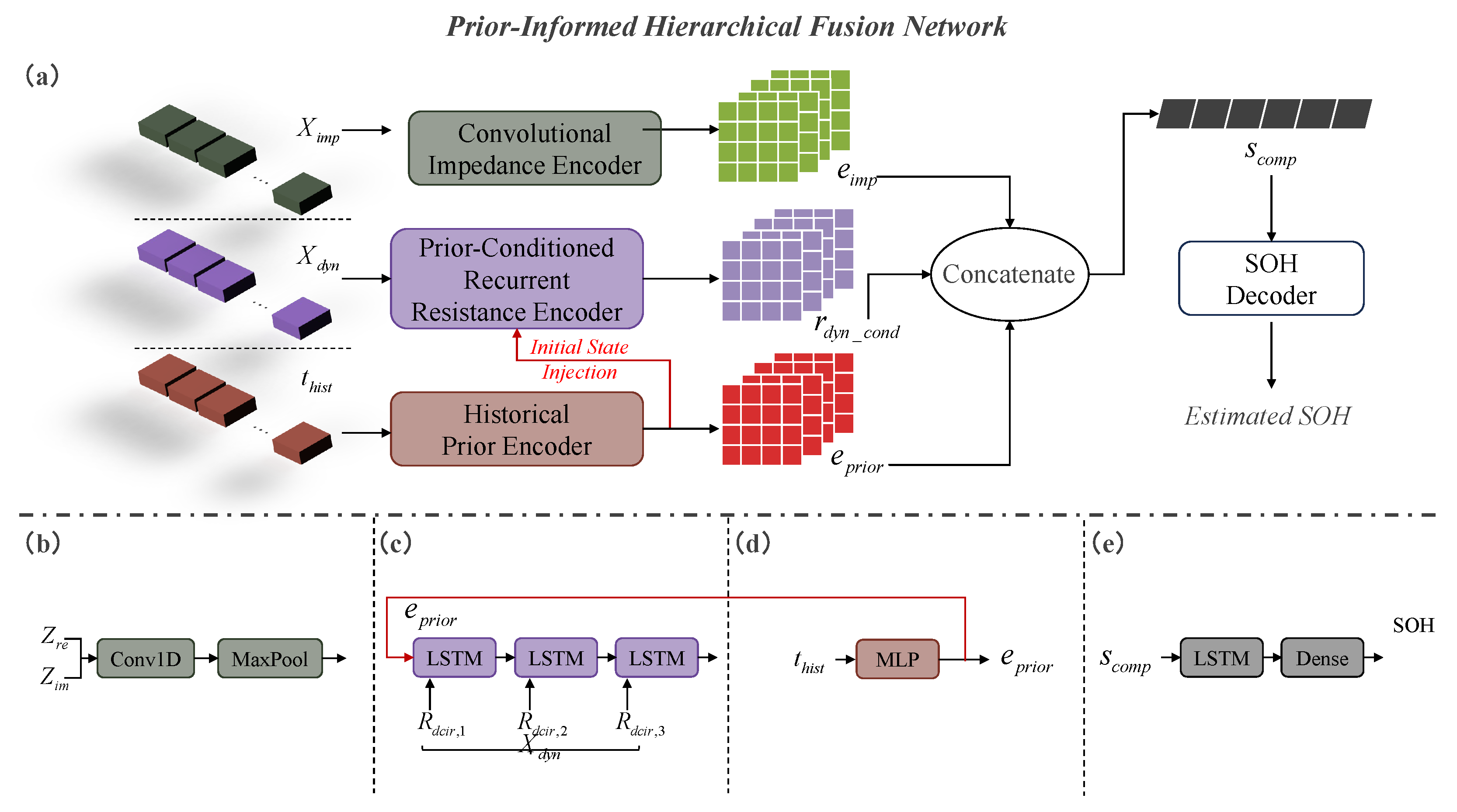
The information processing flow within the network embodies its core hierarchical fusion concept. Initially, the historical degradation trajectory vector, , is fed into the prior encoder to generate a historical prior embedding that encapsulates the battery’s cumulative aging information. This embedding subsequently serves as a conditional signal, utilized to initialize the state of the recurrent neural network that processes the dynamic resistance sequence, . This mechanism ensures that the interpretation of the present dynamic behavior is directly guided by its historical context. Concurrently, the other branch of the parallel state encoder processes the electrochemical impedance spectrum, , to extract its deep features in the frequency domain. Finally, these two feature streams, one representing the history-conditioned dynamic response and the other representing the instantaneous impedance characteristics, are fused into a comprehensive state representation. This representation is then mapped by the decoder to an accurate SOH estimate. The complete architecture of the proposed PI-HFN is visually detailed in Figure 1.
Figure 1.
The overall architecture of the PI-HFN: (a) The information flow from the three heterogeneous inputs through the encoders, fusion module, and decoder to the final SOH output; (b) Internal structure of the Convolutional Impedance Encoder; (c) Details of the Prior-Conditioned Recurrent Resistance Encoder; (d) Structure of the Historical Prior Encoder; (e) Internal components of the SOH Decoder.
2.2. Input Data Definition and Preprocessing
The inputs to the PI-HFN model are composed of three heterogeneous data groups, which characterize the battery’s instantaneous electrochemical properties and its cumulative aging history, respectively. This section formally defines these three input data groups and describes the standardized preprocessing procedures employed to ensure model training stability.
The first input group consists of instantaneous electrochemical measurements, which includes both the electrochemical impedance spectrum and the dynamic resistance sequence. The electrochemical impedance spectrum, , is acquired by applying a sinusoidal perturbation signal to the battery over a specific frequency range . At K discrete frequency points , each measurement is a complex number . To facilitate processing by the convolutional neural network, this complex sequence is decomposed into two parallel real-valued sequences: the real part of the impedance, , and the imaginary part, . Consequently, the impedance spectrum input to the model is defined as a two-dimensional array, . The dynamic resistance sequence, , is obtained from direct current pulse tests triggered at M predefined operating points. While ideally defined by State-of-Charge (SOC), in practical scenarios—particularly for chemistries with distinct voltage slopes like NMC—these points are defined by terminal voltage thresholds to avoid dependence on capacity estimation. For chemistries with flat voltage plateaus (e.g., LFP), relative SOC points derived from a fully charged state are employed. Thus, the sequence is formally represented as . In practical inference scenarios, the integrity of the dynamic resistance sequence is critical. To handle potential sensor dropouts or data corruption, a validity check is implemented. Isolated missing values within the sequence are reconstructed using linear interpolation based on the adjacent valid SOC points, preserving the vector’s fixed dimensionality. However, to maintain safety standards, if the proportion of corrupted points exceeds a safety threshold, the estimation process is aborted, and a fault flag is raised instead of outputting a potentially unreliable SOH value.
The second input group is the historical degradation trajectory vector, . This vector is designed to summarize the key aging processes and cumulative effects experienced by the battery during its first life-cycle using a refined set of scalar values. It is a fixed-dimensional vector whose composition covers cycle life, charge throughput, end-of-first-life state, and statistical information on operating conditions. The vector is defined as , where D is the total dimension of the historical features. Table 1 provides a detailed description of the specific components of the historical degradation trajectory vector used in this study and their physical significance.
Table 1.
Composition and description of the Historical Degradation Trajectory Vector ().
Physically, the construction of this historical vector is grounded in the battery’s cumulative stress history. The aggregated usage metrics, including total cycle count and throughput, quantify the total extent of electrochemical reactions, serving as a proxy for time-dependent side reactions. Simultaneously, the operating stress conditions, such as temperature and C-rate statistics, reflect the severity of thermal and mechanical loads during the first life. These features provide a physical basis for the subsequent Prior Encoder to learn a high-dimensional embedding that captures the path-dependent nature of degradation, distinguishing batteries with similar electrical states but different aging histories.
All input data undergo a rigorous preprocessing procedure before being fed into the PI-HFN model. This is to eliminate the influence of different physical units and numerical scales, thereby accelerating network convergence and enhancing model performance. This study employs Min–Max Scaling to linearly map the numerical range of all features to the interval [0, 1]. For any given feature value x, its normalized value is calculated using the following equation:
The selection of Min-Max normalization over variance-based scaling methods is driven by two factors specific to this application. First, the electrochemical parameters involved (e.g., voltage response, state of health) possess inherent physical boundaries, making a bounded scaling method physically representative. Second, and critically, the proposed model is designed for deployment on edge AI accelerators (as detailed in Section 3.1.2) which utilize INT8 quantization. Min-Max normalization ensures that the input distribution is strictly confined within a deterministic interval , thereby maximizing the dynamic range usage of the quantization parameters and preventing the overflow or clipping issues associated with unbounded standardization methods.
It is crucial to note that the scaling parameters, and , are determined based exclusively on the statistical distribution of the training dataset. These parameters are then fixed and applied consistently to the validation and test datasets during the model evaluation phase. This practice ensures uniformity in data processing and prevents any information leakage from future data. Finally, to address the potential risk of data leakage, particularly when historical information is incomplete or requires estimation, the construction of the historical degradation trajectory vector follows a strict principle of temporal isolation. All elements within are derived exclusively from data recorded prior to the initialization of the second-life phase. In scenarios where historical parameters must be estimated due to data loss, the estimation relies solely on snapshot characterization at the transition point between the first and second lives.
2.3. PI-HFN Model Architecture Details
The core architecture of the PI-HFN model is composed of three specialized encoder modules, which are responsible for processing the impedance spectrum, historical trajectory, and dynamic resistance sequence, respectively. These modules work in concert to achieve an effective transformation from multi-modal inputs to a prior-conditioned feature representation.
2.3.1. Convolutional Impedance Encoder
The objective of the Convolutional Impedance Encoder is to autonomously learn and extract hierarchical frequency–domain features directly from the raw two-dimensional impedance spectrum matrix, . The main body of this encoder consists of a series of stacked one-dimensional convolutional (Conv1D) layers, non-linear activation layers, and pooling layers. The 1D convolution operation computes a feature map by sliding a learnable kernel across an input sequence , a process formally expressed as:
where M is the size of the kernel. Each convolutional layer is followed by a Rectified Linear Unit (ReLU) activation function to introduce non-linearity. Through the stacking of multiple convolutional layers, the network can construct a feature hierarchy from low-level local patterns to high-level global shapes. To obtain a fixed-dimensional feature representation, a Global Average Pooling layer is employed at the end of the encoder. This layer averages the feature maps from the last convolutional layer across the frequency dimension. This process ultimately yields a compact feature vector, which we define as the Impedance Spectrum Embedding, , summarizing the core information of the entire impedance spectrum. To transition from the local feature maps extracted by the convolutional layers to a compact representation, a Global Average Pooling (GAP) layer is employed. Physically, while the convolutional filters identify localized electrochemical patterns across the frequency domain. By calculating the average response of each feature map, the GAP layer aggregates these localized shape activations into a global intensity metric. This operation creates a fixed-dimensional vector quantifies the overall prominence of various degradation patterns regardless of their specific positions along the frequency axis, thereby reducing the model’s sensitivity to frequency shifts or input length variations.
2.3.2. Historical Prior Encoder
The Historical Prior Encoder is responsible for processing the low-dimensional yet information-dense Historical Degradation Trajectory vector, . Its primary function is to map this engineered feature vector into a higher-dimensional latent space, enabling it to serve effectively as prior conditional information. Given that is a structured vector of scalars, this study employs a Multi-Layer Perceptron (MLP) as its encoder. The MLP consists of several fully-connected layers, each followed by a non-linear activation function. The forward propagation process for the l-th layer can be expressed as:
where is the output of the l-th layer (with ), and are the weight matrix and bias vector of the layer, respectively, and is the non-linear activation function. Through this MLP, the model can learn the complex non-linear relationships among the historical features. The final output vector of the encoder is defined as the Historical Prior Embedding, , which will act as a conditioning signal for the subsequent module.
This projection mechanism renders the framework highly scalable regarding the dimensionality of historical data. Since the Prior Encoder acts as a dimensionality interface, extending the input vector with additional historical features only requires adjusting the input layer size of the MLP. The subsequent modules operate on the fixed-dimensional embedding , thereby isolating the downstream architecture from variations in the raw data schema. Furthermore, the computational overhead of processing additional scalar features via an MLP is negligible compared to the convolution and recurrent operations required for the electrochemical inputs.
2.3.3. Prior-Conditioned Recurrent Resistance Encoder
The Prior-Conditioned Recurrent Resistance Encoder is the key component that actualizes the hierarchical fusion concept of the model. Its task is to process the Dynamic Resistance Sequence, , with its encoding process being directly modulated by the Historical Prior Embedding, . This study employs a Long Short-Term Memory (LSTM) network as the main body of this encoder and implements the conditioning through an Initial State Injection mechanism. Specifically, is not treated as part of the sequence input; instead, it is transformed by two independent fully-connected layers to generate the initial hidden state and initial cell state for the LSTM network:
where are learnable parameters. In this manner, the internal memory of the LSTM is initialized with information encapsulating the battery’s entire historical degradation before processing the first time step of the dynamic resistance sequence. Comparatively, while attention mechanisms are powerful for aligning dynamic sequences, this static injection strategy is theoretically more suitable for integrating fixed historical priors. It avoids the redundant computation of relevance scores at every time step while effectively biasing the entire recurrent reasoning process with a global aging baseline. Subsequently, the LSTM processes the entire sequence according to its standard update equations. At each time step t, the updates to its cell state and hidden state are as follows:
Upon completion of sequence processing, the hidden state of the LSTM at the final time step serves as the feature vector, which has been guided and modulated by the historical information. We define this output as the Conditioned Dynamic Resistance Representation, . Functionally, this Initial State Injection strategy differs from simple input concatenation by utilizing the historical embedding to establish the initial condition of the recurrent network. Physically, this approach reflects the path dependent nature of battery dynamics where the transient response is conditioned by the accumulated degradation state. By initializing the cell memory and hidden state with the historical prior, the model sets a global operating point to calibrate the interpretation of instantaneous resistance variations according to the specific aging history.
2.4. Feature Fusion and SOH Decoding
After the parallel encoder modules generate the Impedance Spectrum Embedding, , and the Conditioned Dynamic Resistance Representation, , the model proceeds to the final stage of feature fusion and regression. This stage is designed to effectively integrate these two high-dimensional feature vectors, which represent the instantaneous impedance characteristics and the history-conditioned dynamic response, respectively, and to decode the final SOH estimate from the resulting representation.
The feature fusion step employs a concatenation operation to join the two feature vectors along their feature dimension, thereby forming a higher-dimensional and more comprehensive feature vector, which we define as the Comprehensive State Representation, . This operation is expressed as:
This fused vector, , contains a multi-faceted, multi-angle description of the battery’s current health state, providing a solid foundation for the subsequent precise regression task. The Comprehensive State Representation is then fed into the SOH decoder. The decoder consists of a LSTM layer followed by a fully-connected (Dense) output layer. Although the fused feature vector is non-sequential, the decoder employs an LSTM unit to leverage its internal gating mechanisms. Unlike a standard fully-connected layer, these gates provide a capability for selective information filtering. They enable the model to dynamically regulate the information flow from the high-dimensional fused representation, effectively suppressing noise and emphasizing the most relevant features from both historical and instantaneous inputs before the final regression step. This vector is immediately passed to the fully-connected layer. This output layer contains only a single neuron and utilizes a linear activation function to ensure that the model’s output is an unbounded, continuous value that can directly correspond to the physical range of SOH. With this, the entire end-to-end mapping from multi-modal inputs to a single-valued SOH output is fully realized.
2.5. Model Training and Evaluation
The proposed PI-HFN model is trained end-to-end using a supervised learning paradigm. The entire set of network parameters, collectively denoted as , is optimized by minimizing the Mean Squared Error (MSE) loss function, , between the predicted and true SOH values. This loss function is defined as:
where N is the number of samples in a training batch, is the model’s prediction for the i-th sample, and is its corresponding ground-truth label. The parameter optimization is carried out using the backpropagation algorithm and the Adam optimizer. To ensure the generalization capability of the model and to prevent overfitting, the dataset is partitioned into independent training, validation, and test sets. The validation set is used for model selection and for tuning key hyperparameters during the training process, while the test set is reserved for a single, unbiased evaluation of the final trained model’s performance. To comprehensively assess the model’s performance, this study adopts three standard regression evaluation metrics: Root Mean Squared Error (RMSE), Mean Absolute Error (MAE), and the Coefficient of Determination ().
where is the mean of the true SOH values. Together, these metrics will provide a quantitative assessment of the accuracy and reliability of the model’s predictions.
3. Experimental Validation and Results
3.1. Case Study 1: Validation with Multimodal EIS and DCIR Data (Stanford NMC)
3.1.1. Dataset, Model Setup, and Experimental Design
All data utilized in this study were sourced from a publicly available dataset released by the Stanford Energy Control Laboratory [19,20,21]. This dataset provides continuous aging records for the same batch of lithium-ion cells from their first life (1L) to their second life (2L), offering an ideal data foundation for investigating the influence of historical information on the state-of-health estimation for second-life applications. The 1L phase data, based on electric vehicle driving conditions, is used to construct a unique historical degradation trajectory vector for each cell. The 2L phase data, based on grid energy storage application cycles, provides the instantaneous electrochemical measurements and the corresponding ground-truth state-of-health values required for training and validating the proposed model.
The experimental subjects are commercial LG Chem INR21700-M50T (LG Energy Solution, Seoul, Republic of Korea) cylindrical lithium-ion cells, which feature a Nickel–Manganese–Cobalt cathode and a graphite–silicon composite anode. The nominal capacity of these cells is 4.85 Ah, and the nominal voltage is 3.63 V. The dataset completely documents two critical life stages of the batteries, from brand new to the end of their second life. In the first-life stage, a total of ten new cells underwent a 23-month aging experiment in a temperature-controlled environment at 23 °C. The cycling protocol for this stage utilized the Urban Dynamometer Driving Schedule (UDDS) as the discharge profile to simulate realistic electric vehicle driving scenarios. In the second-life stage, six cells selected from the previous stage were subjected to a further 24 months of aging experiments. The cycling protocol for the 2L stage simulated the application scenarios of residential and commercial grid energy storage systems, with the cycling temperature alternating between 20 °C and 35 °C to mimic seasonal temperature variations. This two-stage experimental design furnishes a valuable dataset for this research, making it possible to extract the aging history of each cell from the 1L data and to validate the model’s ability to utilize this historical information for state-of-health estimation on the 2L data.
The historical degradation trajectory vector quantitatively summarizes the aging process and cumulative effects experienced by each cell during its first life cycle. This vector consists of a series of key scalar metrics extracted or calculated from the 1L dataset. This information primarily includes the total number of accumulated cycles, charge rate, and final state of capacity at the end of the first life cycle. Details are described in Section 2.2. This vector provides the model with basic prior knowledge of each cell’s degradation history. Before input into the model, all elements in the vector are min-max normalized.
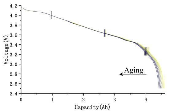
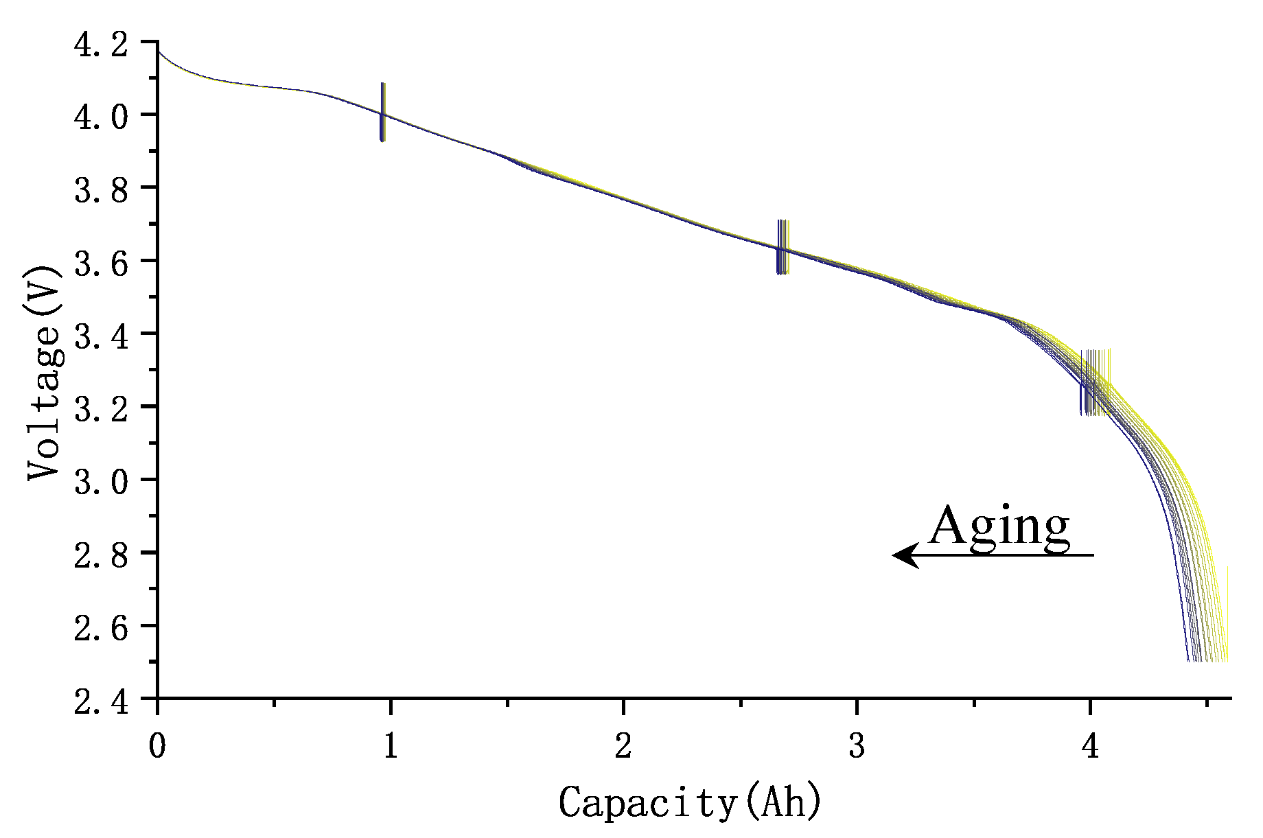
The Secondary Life dataset provides the core data for training, validating, and testing the models used in this study. This dataset contains two types of impedance data collected during the Secondary Life Reference Performance Tests (RPTS) and their corresponding true SOH values. The true SOH is calibrated using capacity tests performed during each RPT. These tests involve fully discharging the battery at a constant C/20 current. The discharge capacity, , is calculated by integrating the current over time, the degradation of which is visualized for a representative cell in Figure 2. The SOH is then defined as the percentage of the current discharge capacity to the battery’s initial nominal capacity, .
Figure 2.
Discharge capacity degradation curves for battery V4 over successive RPTs (Case Study 1). The color evolution of the curves corresponds to the progression of battery aging. The leftward shift of the curve indicates capacity fade, which is the primary aging phenomenon quantified by the SOH. Each curve represents a full discharge test used to determine the ground-truth SOH value ().
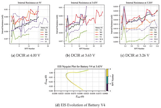
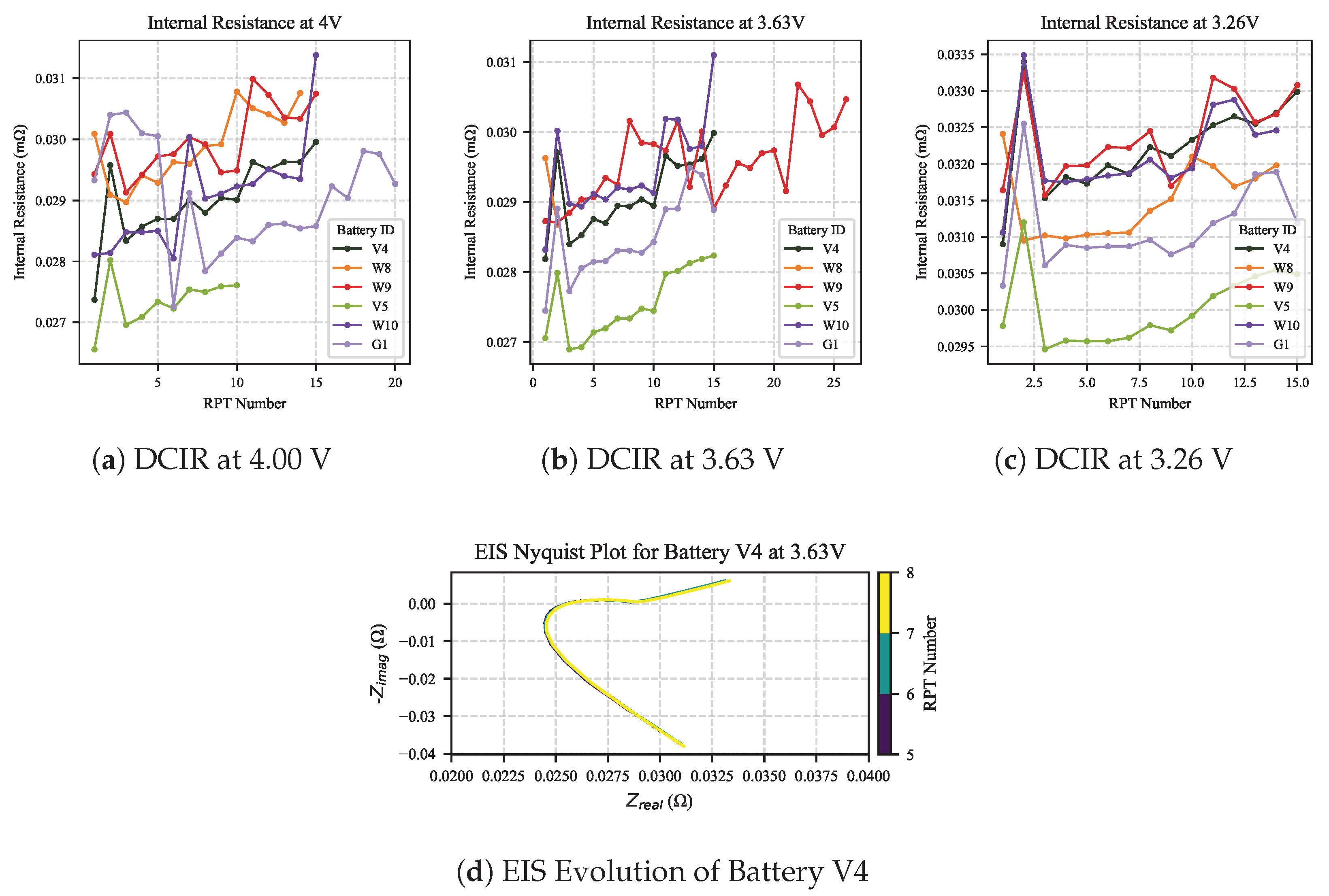
The model’s instantaneous electrochemical inputs, namely the impedance spectrum and the dynamic resistance sequence , are also acquired during the RPTs. As illustrated in Figure 3, these inputs capture the battery’s state at different points in its second life. EIS measurements (Figure 3d) are conducted over a frequency range of 0.01 Hz to 10 kHz at three distinct voltage levels: 4.00 V, 3.63 V, and 3.26 V. The collected complex impedance data are decomposed into their real and imaginary part sequences to form the input matrix . Data for the dynamic resistance sequence, , are derived from pulse tests. At the same three voltage levels, the cell is subjected to a C/2 discharge pulse, and the resulting DCIR values (shown in Figure 3a–c) constitute the input sequence . Similar to the historical trajectory vector, both and are subjected to min-max normalization before being fed into the model.
Figure 3.
Visualization of the instantaneous electrochemical input features (Case Study 1). (a–c) The evolution of DCIR for all six cells measured at three different voltage levels throughout their second life, corresponding to the input vector . (d) The evolution of the EIS for battery V4 across multiple RPTs, illustrating the data structure of the input matrix .
To provide a more comprehensive and robust evaluation of the models’ generalization capabilities and to mitigate the potential biases arising from a single, fixed data split, this study adopts a 3-fold cross-validation strategy. This strategy strictly adheres to the principle of a cell-wise split, meaning that for each fold of the validation, the data is partitioned at the battery cell level to completely prevent data leakage. Given the six independent cells available in the second-life dataset, we divided these cells into three distinct groups, with each group containing two cells. In each fold of the cross-validation, one group was held out as the independent test set, while the remaining two groups were combined and used for model training and validation. The specific partitioning scheme is as follows: in the first fold, cells G1 and V4 served as the test set; in the second fold, cells V5 and W8 were used as the test set; and in the third fold, cells W9 and W10 constituted the test set. The model was trained, validated, and tested independently for each fold. The final reported performance of the models, such as RMSE and R2, is the average of the test results across all three folds, thereby providing a more reliable and statistically significant assessment of the models’ generalization performance.
The implementation and training of all models in this study were conducted in a unified software and hardware environment to ensure the fairness of the comparative experiments. The experimental platform was based on the Python 3.9 programming environment, utilizing the PyTorch 2.1 deep learning framework for network construction and training. All computational tasks were executed on a high-performance workstation equipped with an NVIDIA A40 GPU featuring 48 GB of GDDR6 memory. Regarding the specific hyperparameters of the PI-HFN model, the Convolutional Impedance Encoder was constructed with three stacked 1D convolutional blocks, with filter counts of 32, 64, and 128, respectively. Each used a kernel size of 3 and was followed by a ReLU activation function and a max-pooling layer with a pool size of 2. The Historical Prior Encoder was a Multi-Layer Perceptron with two hidden layers containing 64 and 32 neurons, respectively, also using ReLU activation. Both the Prior-Conditioned Recurrent Resistance Encoder and the final SOH Decoder utilized a single-layer LSTM network with 128 hidden units, followed by a Dropout layer with a rate of p = 0.2 to mitigate overfitting. For the training configuration, all models were optimized using the Adam optimizer with an initial learning rate of 0.001 and default beta parameters (). A learning rate decay strategy was employed, reducing the learning rate by a factor of 0.1 if the validation loss did not improve for 5 consecutive epochs. The models were trained for a maximum of 200 epochs with a batch size of 64. Furthermore, to prevent overfitting and select the optimal model, an early stopping mechanism was implemented, monitoring the validation set loss with a patience of 15 epochs.The specific patience value of 15 epochs was selected empirically based on preliminary training trials. This window was found to provide a sufficient buffer to distinguish between transient stochastic fluctuations in the validation loss and a genuine trend of overfitting, thereby preventing premature termination while ensuring the model converges to a robust optimum.
To systematically validate the performance advantages and core innovations of the proposed PI-HFN model, a series of comparative experiments were designed (Table 2). By constructing models with varying architectures or input information, the respective contributions of historical information and the hierarchical fusion strategy can be quantitatively analyzed. In addition to the primary PI-HFN model, three comparative models were introduced: a Parallel Fusion Network (PFN), a Baseline Fusion Network (BFN), and a Gradient Boosting Regression Tree (GBRT) model. The PFN is used for an ablation study to validate the effectiveness of the hierarchical fusion strategy. It possesses the same three independent encoders as the PI-HFN but employs a simple late concatenation to fuse all encoded features, instead of a prior-conditioning mechanism. The BFN is also used for an ablation study, aiming to quantify the value of first-life historical information. This model entirely omits any historical information, relying solely on instantaneous electrochemical measurements for estimation. Finally, the GBRT model serves as a traditional machine learning baseline to compare the end-to-end deep learning method against a conventional feature-engineering approach. Its input is a 9-dimensional feature vector composed of three sets of features extracted at different voltage points: the ohmic resistance () and charge-transfer resistance () obtained from an equivalent circuit model fit, and the raw direct current internal resistance () values.
Table 2.
Summary of Comparative Models (Case Study 1).
3.1.2. Results, Ablation Analysis, and Computational Cost (Case Study 1)
This part aims to provide a comprehensive evaluation and analysis of the performance of the proposed PI-HFN model and other comparative models for this case study. First, based on the results from a 3-fold cross-validation, we will independently demonstrate the high-precision performance of the PI-HFN model in the task of SOH estimation for 2L batteries and visually analyze its capability to track true degradation trajectories. Subsequently, by summarizing the average performance metrics from the cross-validation, a quantitative performance comparison and in-depth ablation study against the PFN, BFN, and GBRT will be conducted to validate the effectiveness of the hierarchical fusion strategy and historical information proposed in this study. Finally, this chapter will also assess the computational cost of the PI-HFN model on different hardware platforms to analyze its deployment potential in practical applications.
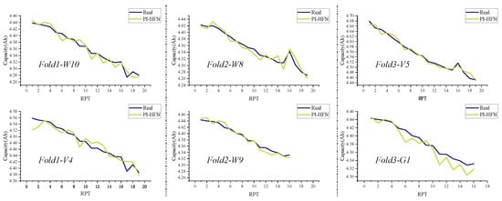
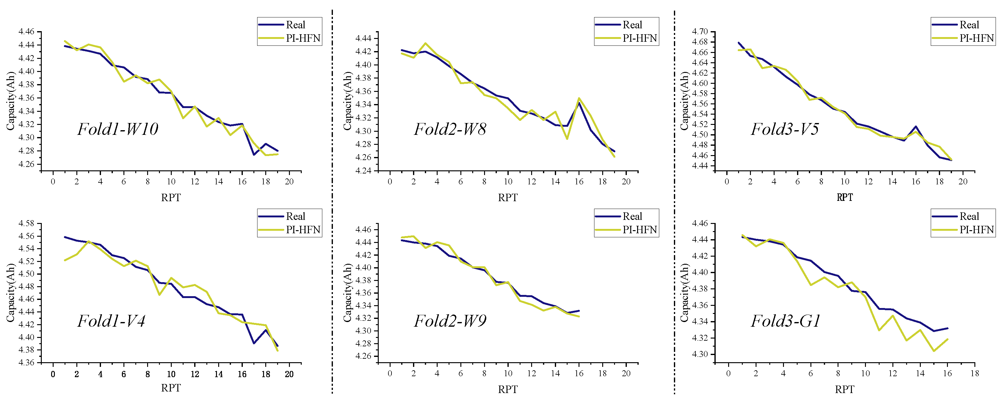
To independently evaluate the generalization performance of the proposed PI-HFN model, its estimation results from the 3-fold cross-validation process were visualized. Figure 4 presents the SOH estimation trajectories for all six battery cells, where the prediction curve for each cell was generated by the model trained in the specific fold where that cell was part of the hold-out test set. For instance, the prediction results for cells G1 and V4 are from the model trained in Fold 1, the results for V5 and W8 are from the model trained in Fold 2, and the results for W9 and W10 are from the model trained in Fold 3.
Figure 4.
Visual comparison of SOH estimation results across the 3-fold cross-validation. The subplots are organized by test folds. The results demonstrate consistent tracking performance across different data partitions.
As can be clearly observed from the figure, the PI-HFN model demonstrates excellent and consistent performance across all three folds of the validation. For every cell, regardless of which fold it was assigned to as a test set, the model’s prediction curve aligns closely with the real degradation trajectory, accurately capturing the overall downward trend of capacity fade with aging. This result provides strong evidence of the model’s robust generalization capability, as it indicates that the model’s high performance is not coincidental to a specific test set partition. Instead, it consistently learns universal electrochemical aging features under different training/testing data combinations and successfully applies them to unseen cells. Furthermore, despite the fact that different cells exhibit varied degradation rates and behaviors due to their distinct 1L experiences, the PI-HFN model is capable of providing accurate, individualized tracking for the respective test cells in each fold. The observed estimation deviation in the late aging stage is likely attributable to accelerated degradation phenomena, specifically lithium plating and active material loss. While DCIR and EIS effectively characterize impedance rise and interfacial stability, their sensitivity to the onset of inactive lithium formation remains limited. Consequently, the model exhibits a prediction bias when these specific electrochemical behaviors precipitate rapid capacity fade that is not linearly reflected in the resistance evolution.
To quantitatively validate the superiority of the PI-HFN model and to elucidate the contributions of its key designs, namely the historical information and the hierarchical fusion strategy, this section summarizes the average performance metrics of all comparative models from the 3-fold cross-validation. The detailed performance comparison results are presented in Table 3.
Table 3.
Comparative Performance (Mean ± Std. Dev.) in 3-Fold Cross-Validation (Case Study 1).
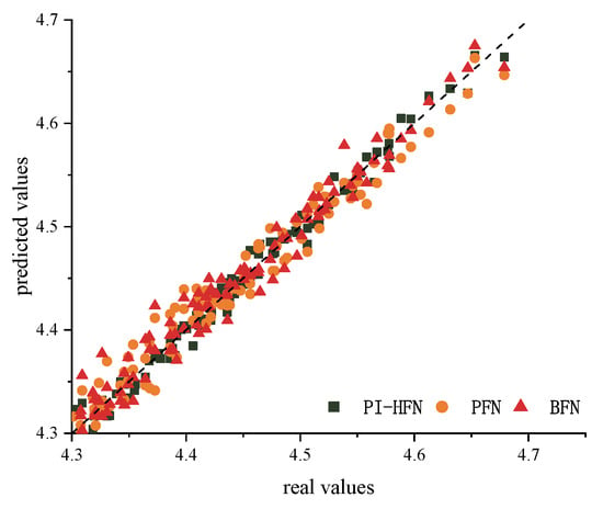
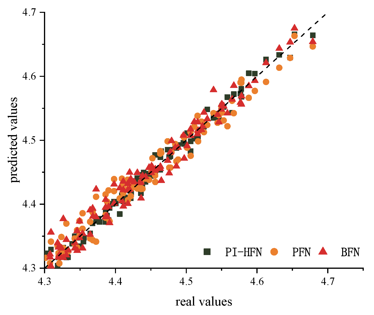
The results in the table clearly show that the proposed PI-HFN model achieves the best estimation performance among all comparative methods, attaining the lowest average RMSE of 1.91% and the highest average Coefficient of Determination (R2) of 0.990 across the three test folds. To isolate and validate the effectiveness of the hierarchical fusion strategy, the PI-HFN was compared against the PFN, which employs a simple late fusion. The PFN achieved an average RMSE of 2.13%, a noticeable performance gap compared to the PI-HFN. This strongly demonstrates that the hierarchical fusion architecture using prior-conditioning via initial state injection is more effective at leveraging historical information to guide the interpretation of the current electrochemical state. This performance gap suggests that simply providing historical data as another parallel input is less effective. The true advantage comes from the hierarchical conditioning, where the historical prior actively modulates the network’s interpretation of dynamic electrochemical behavior, which aligns better with the underlying physical degradation processes. This superior performance is visually confirmed in Figure 5, where the predictions of the PI-HFN model exhibit the tightest clustering along the ideal line compared to the other models.
Figure 5.
Scatter plot of predicted versus true SOH values for the PI-HFN, PFN, and BFN models (Case Study 1) on the combined test sets from the 3-fold cross-validation. The dashed line represents the ideal y = x line where predicted values equal true values. The tight clustering of PI-HFN points along this line indicates its superior accuracy.
To quantitatively validate the superiority of the PI-HFN model and ensure the results are statistically robust, we summarize the average performance metrics and their standard deviations across the 3-fold cross-validation. Detailed statistics are presented in Table 3.
The PI-HFN model achieves the lowest average RMSE of 1.91% (±0.25%) and the highest of 0.990 (±0.002). The small standard deviation indicates that the model is insensitive to data partitioning and generalizes well. Comparatively, the BFN shows a much higher error and variance (). A paired t-test performed on the fold-wise RMSEs of PI-HFN and BFN yields a p-value , confirming that the accuracy improvement provided by the historical prior is statistically significant.
To justify the architectural hyperparameters of the Convolutional Impedance Encoder, we conducted a sensitivity analysis on the kernel size and network depth. We performed a grid search comparing varying depths from two to four layers and kernel sizes from three to seven. As summarized in Table 4, the performance exhibits a clear non-monotonic trend. The shallow configuration with two layers resulted in a higher RMSE of 2.15%, indicating insufficient capacity to capture high-level abstract features from the impedance spectrum. Conversely, increasing the depth to four layers led to a slight performance degradation to 1.98%, attributed to overfitting on the limited dataset. Regarding the receptive field, the model with a kernel size of 3 consistently outperformed those with larger kernels of 5 and 7, suggesting that smaller kernels are more effective at capturing the fine-grained local variations in the EIS frequency domain. Therefore, the architecture with three layers and a kernel size of 3 was selected as the optimal configuration.
Table 4.
Sensitivity analysis of CNN hyperparameters (Depth and Kernel Size).
To assess robustness under non-ideal data conditions, we conducted a sensitivity analysis on historical data availability and accuracy. Two feature ablation schemes were designed: Variant A excludes hard-to-measure features (), while Variant B retains only three fundamental counters ().
As shown in Table 5, Variant A’s RMSE increased slightly to 2.02%, confirming minimal reliance on internal resistance. The minimalist Variant B maintained a stable RMSE of 2.32%, significantly outperforming the history-free BFN (3.57%), validating the value of limited historical statistics. This hierarchical performance comparison also provides a quantitative decomposition of feature contributions: the basic accounting features () serve as the primary drivers, contributing approximately 75% of the total performance gain derived from historical data, while the detailed statistical features () act as auxiliary refinements for precision fine-tuning.
Table 5.
Ablation study results on the availability of historical features.
Furthermore, a noise sensitivity test was performed on Variant B by injecting Gaussian noise (). As detailed in Table 6, the RMSE exhibits only marginal increases. Even with 20% noise, the error (2.59%) remains well below the BFN baseline, demonstrating the model’s strong tolerance to input uncertainty.
Table 6.
Sensitivity analysis of Variant B under varying noise levels.
To evaluate deployment feasibility under hardware constraints, we tested two scenarios: Sparse EIS and No EIS. In the Sparse EIS setting, we retained only 100, 1, and 0.1 Hz to represent key impedance regions. In the No EIS setting, we relied solely on DCIR and historical priors. As shown in Table 7, the Sparse model achieves 2.05% RMSE, a marginal decline from the 1.91% baseline. Even in the No EIS setting, the RMSE of 2.38% remains significantly superior to the history-free BFN at 3.57%, confirming the model reliability when EIS hardware is limited or unavailable.
Table 7.
Impact of EIS frequency point reduction and availability on model accuracy (Case Study 1).
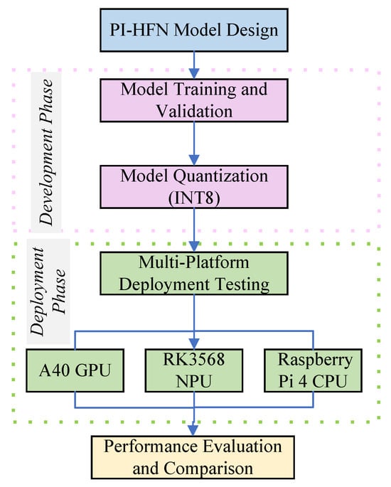
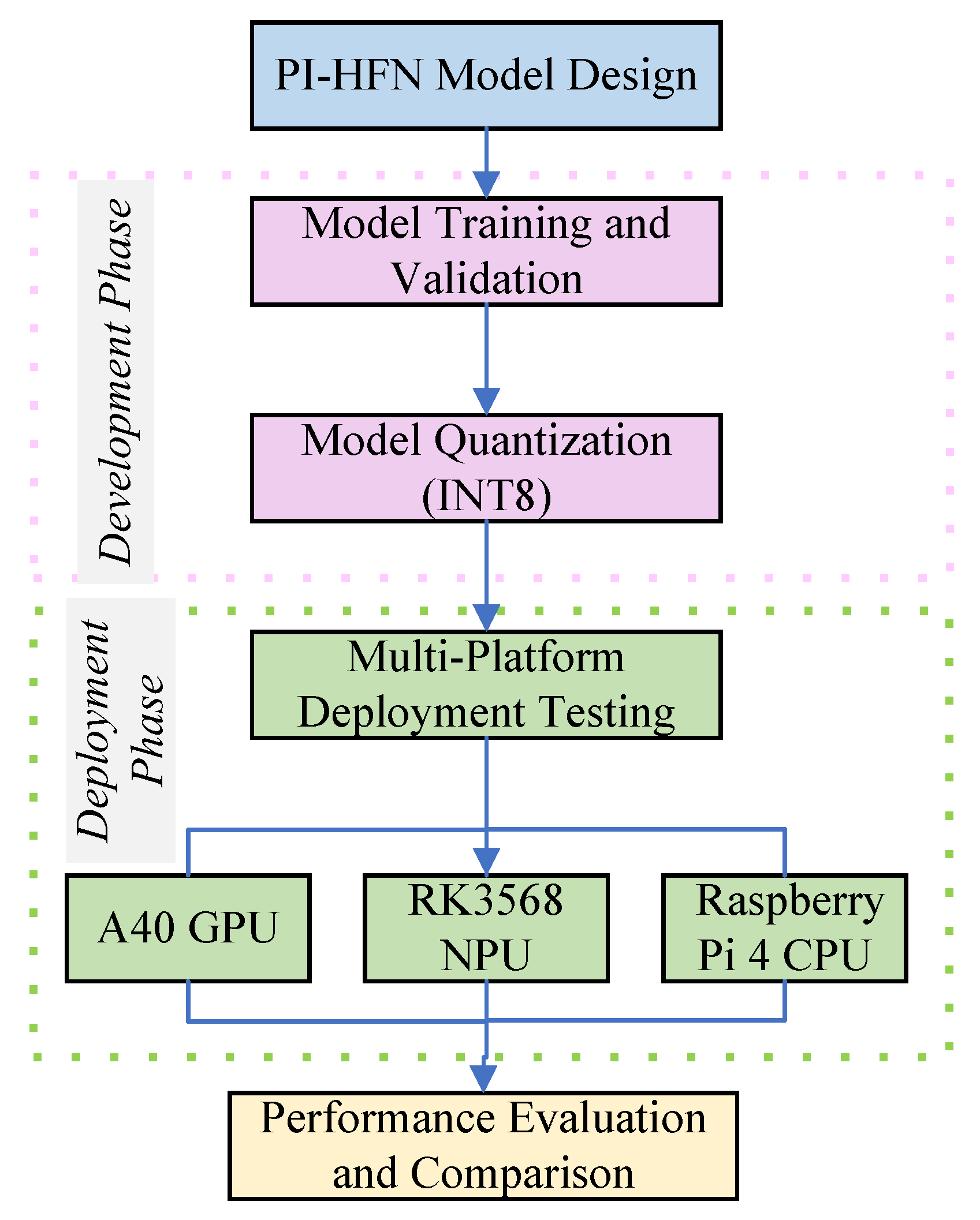
It is important to note that the proposed hierarchical fusion strategy introduces negligible computational overhead compared to the parallel fusion baseline (PFN). Since the historical prior is integrated via initial state injection—effectively replacing the standard zero-initialization of the LSTM—rather than adding complex attention modules or extra layers, the increase in floating-point operations (FLOPs) and parameter count is virtually zero. This structural efficiency ensures that the significant accuracy improvement (RMSE reduction from 2.13% to 1.91%) is achieved without incurring any penalty in inference speed. Beyond estimation accuracy, the deployment feasibility of a model in practical applications is critically important, which primarily depends on its computational cost on various hardware platforms. This section systematically evaluates the inference performance of the proposed PI-HFN model on three representative hardware platforms: a high-end NVIDIA A40 GPU for performance benchmarking, an RK3568 embedded platform representing modern edge AI computing capabilities, and a Raspberry Pi 4 platform representing resource-constrained environments. To fully utilize the integrated Neural Processing Unit (NPU) on the RK3568 platform, the PI-HFN model was first exported from PyTorch format to ONNX, and subsequently converted to an INT8 quantized RKNN format using Rockchip’s toolchain. Photos of the Raspberry Pi 4 and RK3568 are shown in Figure 6.
Figure 6.
The complete pipeline of PI-HFN model: model design, training, quantization, multi-platform deployment, and performance evaluation.
The computational cost and performance evaluation results for the PI-HFN model on each platform are summarized in Table 8. Regarding model size, the original PI-HFN model has a size of 15.2 MB; after INT8 quantization, the model deployed on the RK3568 NPU is significantly reduced to 3.8 MB, demonstrating substantial optimization of storage resources through quantization. Simultaneously, the RMSE of the quantized model on the test set increased marginally from 1.91% to 1.95%, indicating the model’s robustness to the quantization process with negligible accuracy loss. In terms of inference latency, the A40 GPU set a high-performance benchmark with an ultra-low latency of 2.6 ms. The RK3568 NPU demonstrated excellent performance, with an inference latency of merely 15.8 ms, which fully meets the real-time requirements for applications such as in-vehicle or energy storage Battery Management Systems. In contrast, running on the general-purpose CPU platform of Raspberry Pi 4 resulted in an inference latency of 152.1 ms, highlighting the significant advantage of NPUs in edge AI inference. For memory footprint, the model’s peak memory usage on the RK3568 and Raspberry Pi 4 platforms was 85.5 MB and 88.2 MB, respectively, which is entirely acceptable for the memory resources of modern embedded devices. In summary, the PI-HFN model not only achieved optimal accuracy but also demonstrated excellent deployment potential on modern edge AI hardware, exemplified by the RK3568 NPU, achieving a balance between high accuracy and high efficiency.
Table 8.
Computational Cost and Performance Evaluation of the PI-HFN Model (Case Study 1).
It is acknowledged that the sample size of six cells in the second-life phase is limited. Therefore, this case study serves primarily as a depth-first validation, utilizing high-dimensional data to verify the model’s internal mechanisms. The assessment of the framework’s broader generalizability to different chemistries and larger populations is reserved for Case Study 2, which employs a significantly larger dataset of 108 LFP cells.
3.2. Case Study 2: Validation on LFP Cells Without EIS Data
3.2.1. Dataset and Input Definition
To further validate the core thesis of this study and to test the robustness of the proposed framework, a second case study was conducted. This study utilizes the UConn-MathWorks LFP/Gr Second-Life Battery Aging Dataset [21]. This dataset provides a significant complementary validation, featuring a large-scale cohort of 108 commercial LFP cells, which contrasts with the NMC chemistry used in Case Study 1. The experimental design is highly aligned with the research objective, providing clear data partitioning between a 1L of fast-charge-protocol aging and a 2L of 0.5C cycling.
A critical distinction in this dataset is the composition of the instantaneous electrochemical inputs. EIS measurements are not available for these cells; therefore, the input is omitted. However, this dataset provides a more feature-rich characterization of dynamic resistance. The dynamic resistance sequence, , is composed of DCIR measurements taken at nine distinct SOC points.
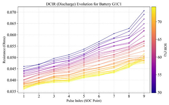
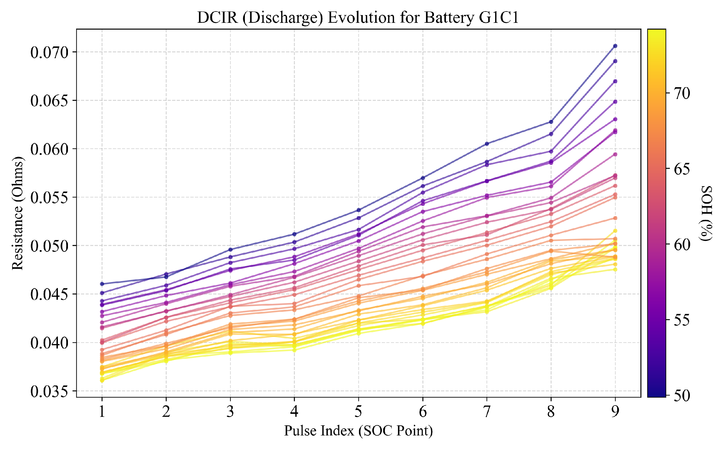
The historical degradation trajectory vector is constructed using the same methodology defined in Section 2.2, summarizing the complete 1L aging process for each cell. Figure 7 illustrates the input data for a representative cell, G1C1. The visualization clearly shows the systematic upward shift of the 9-point DCIR curve as the cell ages and its SOH decreases. This rich, evolving signature serves as the primary instantaneous input for the model in this case study.
Figure 7.
Visualization of the instantaneous electrochemical input for a representative LFP cell, G1C1, in Case Study 2. Each line represents a 9-point DCIR measurement sequence from a single RPT, with the color corresponding to the ground-truth SOH. The plot demonstrates the consistent evolution of the resistance profile with aging.
3.2.2. Model Adaptation and Experimental Design
Given the absence of , the PI-HFN framework was adapted by removing the Convolutional Impedance Encoder. The core methodology was retained: the Historical Prior Encoder still processes to generate , which initializes the recurrent encoder’s state via Initial State Injection before it processes the 9-point sequence. The recurrent encoder’s output, , is then passed directly to the SOH Decoder.
This adaptation tests the hypothesis that the hierarchical fusion mechanism and are the dominant factors for accuracy, even without EIS.
To validate this, we replicated the ablation study from Case Study 1, comparing three models. The first is the adapted PI-HFN. The second is a parallel-fusion PFN, which encodes and separately then concatenates their features. The third is a BFN, which uses only and omits all historical information. This design directly quantifies the value of both and the hierarchical fusion strategy. A 10-fold cell-wise cross-validation was employed for the 108 cells.
3.2.3. Results and Discussion
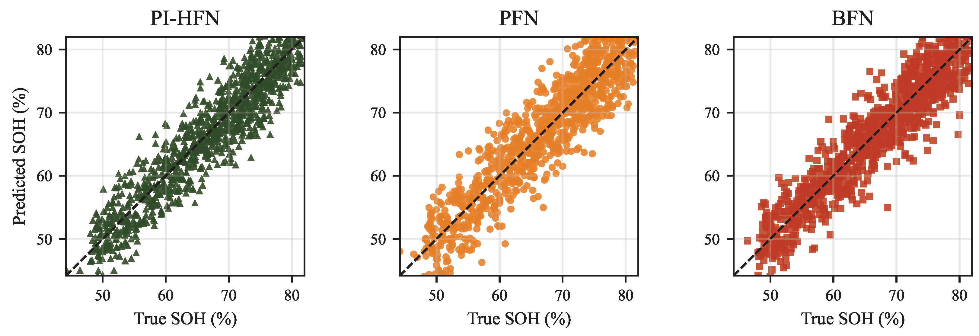
A 10-fold cell-wise cross-validation was employed for the 108 LFP cells. The performance of the three comparative models is visually and quantitatively summarized in Figure 8 and Figure 9.
Figure 8.
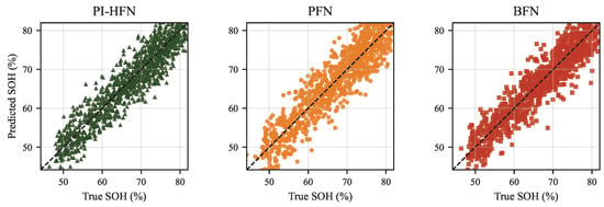
Scatter plot of predicted versus true SOH values for the BFN, PFN, and PI-HFN models (Case Study 2) on the combined 10-fold cross-validation test sets. Although the global trends are similar, the PI-HFN achieves a significantly lower RMSE (1.91%) and tighter variance compared to the PFN (2.13%) and BFN (3.57%), particularly in reducing outliers visible in the BFN subplot.
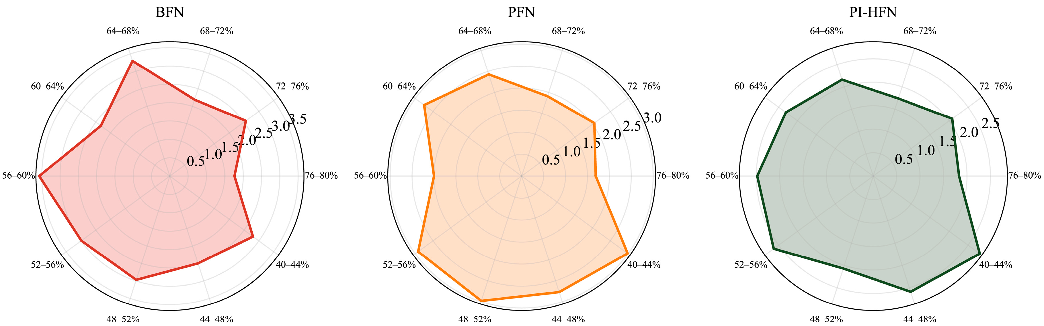
Figure 9.
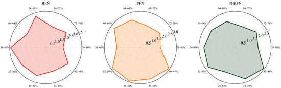
Radar plot comparing model error (e.g., RMSE, MAE) across different SOH sub-intervals. The large spike from the BFN in the 72–76% range highlights its failure in data-sparse regions, a problem significantly mitigated by the PI-HFN.
Figure 8 presents the predicted versus true SOH values for all test sets, organized into three separate subplots for clarity. While all three models reflect the general degradation trajectory associated with the correlation between DCIR and SOH, significant differences in estimation variance are observed. The BFN model, utilizing only DCIR inputs, shows extensive dispersion and outliers, specifically in the rapid degradation region (SOH < 60%) and the data-sparse interval (72–76%). In contrast, the PI-HFN exhibits a condensed clustering along the diagonal reference line. This reduction in variance indicates that the model integrates the historical prior to compensate for the insufficient sensitivity of DCIR measurements in non-linear aging zones, effectively improving the overall estimation accuracy and robustness.
Figure 9 provides a deeper insight into these performance differences by disaggregating the error metrics across SOH sub-intervals. The radar plot for the BFN reveals a severe deficiency, showing a large spike in error, particularly in the SOH 72–76% interval, which corresponds to the “data valley” identified in the SOH distribution. The PFN’s error, while smaller, is also clearly elevated in this same data-sparse region. In sharp contrast, the error profile for the PI-HFN is substantially smaller and more balanced. It effectively suppresses the error spikes in the critical 72–76% region, proving its ability to leverage to overcome the challenge of data sparsity. This confirms that the proposed hierarchical fusion is uniquely effective at providing robust estimations across the entire degradation trajectory.
4. Conclusions
In this study, we addressed the critical challenge of SOH estimation for second-life batteries by proposing the PI-HFN, a flexible deep learning framework that integrates historical first-life data with current electrochemical characteristics. The model’s core innovation is a prior-conditioned hierarchical fusion mechanism, which uses the 1L historical vector to initialize and guide the recurrent encoder processing 2L instantaneous data. The framework’s efficacy was validated across two comprehensive case studies. In Case Study 1 on NMC cells using multimodal EIS and DCIR inputs, the PI-HFN achieved a superior average RMSE of 1.91%. More importantly, Case Study 2 on a large-scale LFP dataset without EIS data demonstrated the framework’s robustness and flexibility. This second study confirmed that is the dominant factor for estimation accuracy, and that the proposed hierarchical fusion strategy was uniquely effective at mitigating the severe estimation errors observed in data-sparse SOH regions where baseline models failed. Through systematic ablation studies, we quantitatively confirmed that removing the historical prior, BFN, or simplifying the fusion architecture, PFN, led to a notable degradation in accuracy. Furthermore, the model’s practical viability was confirmed, achieving a low inference latency of 15.8 ms on an RK3568 edge platform after INT8 quantization. In conclusion, this work provides a robust, accurate, and efficient solution by demonstrating how to effectively leverage limited historical data as a powerful conditional prior, offering a valuable and generalizable tool for the reliable assessment of used batteries. Finally, regarding deployment flexibility, it should be noted that while the proposed PI-HFN architecture is methodologically universal, direct generalization across different battery manufacturers without retraining is not guaranteed due to inherent variations in cell formats and electrochemical baselines. Practical deployment across diverse manufacturers would ideally employ a transfer learning strategy, where the model pre-trained on one cell type is fine-tuned on a small subset of data from the target battery type to align the domain distributions.
Author Contributions
Conceptualization, Y.W.; methodology, Y.W.; validation, Q.W., C.W. and L.W.; investigation, Q.W., C.W. and G.G.; resources, Y.H.; data curation, Y.W., Q.W. and L.W.; writing—original draft preparation, Y.W.; supervision, G.G. and Y.H.; project administration, Y.H. All authors have read and agreed to the published version of the manuscript.
Funding
This research was funded by the 2025 Domestic Visiting Scholar Program for Teacher Professional Development in Higher Education Institutions, grant number FX2025146, and the Special Project for High-level Talents of Huzhou Vocational & Technical College, grant number 2024TS03.
Data Availability Statement
The original contributions presented in this study are included in the article. Further inquiries can be directed to the corresponding author.
Acknowledgments
The authors would like to thank the original data providers for making their dataset publicly available for research purposes.
Conflicts of Interest
The authors declare no conflicts of interest. The funders had no role in the design of the study; in the collection, analyses, or interpretation of data; in the writing of the manuscript, or in the decision to publish the results.
References
- Xu, Q.; Ma, M.; Jiang, T.; Wu, H.; Wang, H. A trustworthy pipeline for data-driven estimation of lithium-ion battery electrochemical impedance spectroscopy using a Physics-Guided Neural Network. J. Energy Storage 2025, 123, 116454. [Google Scholar] [CrossRef] [Scilit]
- Liu, X.; Hu, Z.; Wang, X.; Xie, M. Capacity degradation assessment of lithium-ion battery considering coupling effects of calendar and cycling aging. IEEE Trans. Autom. Sci. Eng. 2023, 21, 3052–3064. [Google Scholar] [CrossRef] [Scilit]
- Daniels, R.K.; Kumar, V.; Chouhan, S.S.; Prabhakar, A. Thermal runaway fault prediction in air-cooled lithium-ion battery modules using machine learning through temperature sensors placement optimization. Appl. Energy 2024, 355, 122352. [Google Scholar] [CrossRef] [Scilit]
- Ma, M.; Xu, Q.; Chen, Q.; Jiang, T.; Wang, H. Interpretable and sensorless lithium-ion battery temperature estimation: A Temporal Fusion Transformer approach. J. Energy Storage 2025, 131, 117414. [Google Scholar] [CrossRef] [Scilit]
- Zhang, Z.; Zhu, Y.; Zhang, Q.; Cui, N.; Shang, Y. Multi-cycle charging information guided state of health estimation for lithium-ion batteries based on pre-trained large language model. Energy 2024, 313, 133993. [Google Scholar] [CrossRef] [Scilit]
- Guenther, L.H.; Klein, V.; Loef, G.; Pohl, A.; Okube, H.; Winterbur, R.; Röwer, G.; Wegener, B.; Goertz, R.; Bracke, S. Second Life for Lithium-Ion Traction Batteries. Sustainability 2024, 16, 7288. [Google Scholar] [CrossRef] [Scilit]
- Li, H.; Wang, S.; Yang, L.; Zhou, Z.; Meng, Y.; Zhang, W.; Shuan, Z.; Li, Y.; Lv, F. SOH estimation method for Lithium-ion battery packs under real-world operating conditions based on a new attenuated model without additional experiments. Energy 2025, 330, 136802. [Google Scholar] [CrossRef] [Scilit]
- Sun, J.; Fan, C.; Yan, H. SOH estimation of lithium-ion batteries based on multi-feature deep fusion and XGBoost. Energy 2024, 306, 132429. [Google Scholar] [CrossRef] [Scilit]
- Chen, X.; Pei, W.; Cui, Z.; Zhang, Q.; Wang, X.; Meng, F.; Li, L. An enhanced hybrid framework of Long short-term memory and transformer networks for Lithium-ion battery health estimation. J. Energy Storage 2026, 148, 120199. [Google Scholar] [CrossRef] [Scilit]
- Antony, A.S.M.; Sundaram, K.M.; Raman, C.J.; Murthy, G.R. Intelligent fault detection in battery systems: A machine learning approach with transformer-enhanced multi-modal Sensing. Electr. Power Syst. Res. 2026, 251, 112279. [Google Scholar] [CrossRef] [Scilit]
- Zhang, X.; Lu, Y.; Shi, J.; Liu, Y.; Cheng, H.; Lu, Y. Dynamic Electrochemical Impedance Spectroscopy: A Forward Application Approach for Lithium-Ion Battery Status Assessment. EcoMat 2025, 7, e70018. [Google Scholar] [CrossRef] [Scilit]
- Zeng, Z.; Mei, B.A.; Song, G.; Hamza, M.; Yan, Z.; Wei, Q.; Feng, H.; Zuo, Z.; Jia, B.; Xiong, R. Physical interpretation of the electrochemical impedance spectroscopy (EIS) characteristics for diffusion-controlled intercalation and surface-redox charge storage behaviors. J. Energy Storage 2024, 102, 114021. [Google Scholar] [CrossRef] [Scilit]
- Pan, B.; Sun, J.; Zhao, X.; Liu, L.; Wang, L.; Pan, C.; Wang, Y. Identification of ohmic internal resistance of batteries based on cloud data. J. Energy Storage 2025, 120, 116364. [Google Scholar] [CrossRef] [Scilit]
- Tao, S.; Guo, R.; Lee, J.; Moura, S.; Casals, L.C.; Jiang, S.; Shi, J.; Harris, S.; Zhang, T.; Chung, C.Y. Immediate remaining capacity estimation of heterogeneous second-life lithium-ion batteries via deep generative transfer learning. Energy Environ. Sci. 2025, 18, 7413–7426. [Google Scholar] [CrossRef] [Scilit]
- Götz, J.D.; Galvão, J.R.; Corrêa, F.C.; Badin, A.A.; Siqueira, H.V.; Viana, E.R.; Converti, A.; Borsato, M. Random forest-based grouping for accurate SOH estimation in second-life batteries. Vehicles 2024, 6, 799–813. [Google Scholar] [CrossRef] [Scilit]
- Zhu, R.; Hu, J.; Peng, W. Bayesian calibrated physics-informed neural networks for second-life battery SOH estimation. Reliab. Eng. Syst. Saf. 2025, 264, 111432. [Google Scholar] [CrossRef] [Scilit]
- Camboim, M.M.; Moreira, A.C.; de Fátima, N.C.; Beck, R.F.; Arioli, V.T.; Omae, C.; Ding, H. State of health estimation of second-life batteries through electrochemical impedance spectroscopy and dimensionality reduction. J. Energy Storage 2024, 78, 110063. [Google Scholar] [CrossRef] [Scilit]
- Guillén Santamaria, J. Comprehensive Analysis of Lithium-Ion Battery Lifecycle and Sustainability in the Automotive Industry: A Perspective of the End of Life in Europe. Ph.D. Thesis, Universitat Politècnica de València, València, Spain, 2024. [Google Scholar]
- Pozzato, G.; Allam, A.; Onori, S. Lithium-ion battery aging dataset based on electric vehicle real-driving profiles. Data Brief 2022, 41, 107995. [Google Scholar] [CrossRef] [Scilit] [PubMed]
- Moy, K.; Khan, M.A.; Fasolato, S.; Pozzato, G.; Allam, A.; Onori, S. Second-life lithium-ion battery aging dataset based on grid storage cycling. Data Brief 2024, 57, 111046. [Google Scholar] [CrossRef] [Scilit] [PubMed]
- Li, T.; Lawlor, A.; Narasimhamurthy, A.; Peng, X.; Hu, C. UConn-MathWorks LFP/Gr Second-Life Battery Aging Dataset. IEEE DataPort 2025. Available online: https://digitalcommons.lib.uconn.edu/reil_datasets/3 (accessed on 23 February 2026).

Disclaimer/Publisher’s Note: The statements, opinions and data contained in all publications are solely those of the individual author(s) and contributor(s) and not of MDPI and/or the editor(s). MDPI and/or the editor(s) disclaim responsibility for any injury to people or property resulting from any ideas, methods, instructions or products referred to in the content. |
© 2026 by the authors. Licensee MDPI, Basel, Switzerland. This article is an open access article distributed under the terms and conditions of the Creative Commons Attribution (CC BY) license.