


Abstract
With the relentless expansion of installed capacity in renewable energy (RE) sources, including wind and photovoltaic power, the operational landscape of the power system has witnessed a substantial surge in uncertainty and complexity. The conventional unit commitment (UC) model falls short when it comes to addressing the challenges posed by a high proportion of RE integration and the collaborative involvement of multiple entities, especially within the electricity market framework. UC now faces a dual challenge: it must not only grapple with the pronounced uncertainty on the source–load side but also harmonize the operational characteristics of emerging entities, such as independent energy storage (ES) systems and virtual power plants. All of this must be achieved while strictly adhering to market regulations and grid safety constraints. To tackle these issues, this paper proposes an intelligent scheduling model built upon a composite neural network. This model enables real-time optimization of scheduling for thermal power, renewable energy, and ES systems through multi-agent collaboration. By doing so, it effectively mitigates the uncertainty associated with RE sources and enhances the safety, economic efficiency, and flexibility of the power system.
1. Introduction
The continuous growth of RE installed capacity, such as wind power and photovoltaics, has resulted in a significant increase in the uncertainty and complexity of power system operation. The conventional UC model has proven to be an ineffective approach in the context of a high proportion of RE grid connections and a diverse range of subjects participating collaboratively [1,2,3]. This is especially evident in the electricity market, where UCs must contend with considerable uncertainty on both the source–load sides. In addition, they are required to coordinate the operational characteristics of novel entities, such as independent ES and virtual power plants (VPPs) [4]. These combinations must also adhere strictly to market rules and grid safety constraints. However, extant research has predominantly concentrated on the collaborative optimization of traditional thermal power and RE sources, with a paucity of systematic incorporation of independent ES, VPPs, and other entities into the prevailing UC decision-making framework [5]. It has also not fully integrated the safety constraint UC logic and the electricity market operation mechanism, resulting in poor adaptability, low decision-making efficiency, and difficulty in ensuring the safety of the model in practical applications.
Against this backdrop, scholars, both domestically and internationally, have conducted in-depth research on the UC problem in multiple dimensions. Reference [6] explored the combination problem involving multiple resource types participating in frequency regulation within transmission-end grids, emphasizing the importance of frequency regulation safety constraints in systems with high renewable energy penetration. Reference [7] systematically reviewed modeling and solution methods for UC in high-penetration renewable energy systems, indicating that stochastic optimization and robust optimization are effective approaches for addressing uncertainty. Reference [8] proposes a two-stage robust UC model accounting for tail risks of wind power forecasting errors, significantly enhancing system operational robustness under extreme scenarios. Reference [9] further introduces control parameter optimization for grid-connected renewable energy, achieving synergistic improvements in frequency regulation safety and economic efficiency through a two-layer model. Reference [10] constructed a two-stage stochastic optimization dispatch model considering source–load uncertainties and incorporates demand response mechanisms, effectively enhancing system flexibility and renewable energy integration capacity.
Despite the considerable progress achieved in uncertainty modeling, frequency constraints and multi-agent collaboration in the aforementioned research, three shortcomings remain [11,12]. Firstly, the operational characteristics and behavior of new entities, such as independent ES and VPPs, have not been systematically integrated. Secondly, there is a lack of adaptation to practical operational constraints, such as the need to operate/maintain units and network congestion in the electricity market. Thirdly, existing models rely heavily on traditional mathematical programming methods, which hinders the achievement of fast and intelligent decision making in high-dimensional and multi-scenario scenarios [13,14,15].
In the context of the rapid development of RE sources, there has been a gradual shift in the power system toward a multi-agent collaborative model of “generation, ES and load network”. The extant research on UCs principally focuses on the collaborative optimization of traditional thermal power and RE sources [16]. However, it is notable that the collaborative effects of RE entities, such as independent ES and VPPs, are largely neglected. Moreover, the integration of safety constraints and market mechanisms within the power system is often ineffective. This article proposes an intelligent decision-making composite neural network (CPNN) model that adapts to the electricity market by combining various emerging energy entities and system security requirements. The enhancement of system flexibility and reliability serves to address the deficiencies observed in traditional models, namely, their poor adaptability and low decision-making efficiency in complex uncertainty scenarios.
2. System Description and Handling of Source–Load Uncertainty
2.1. System Main Body Composition
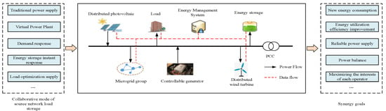
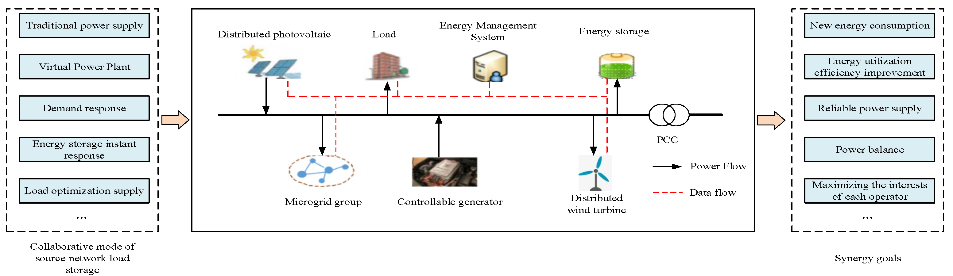
As the electricity market mechanism improves and the proportion of renewable energy rises, the power system is shifting from the traditional “generation follows load” model to a “generation–storage–load–network” multi-agent collaborative model. The high penetration of renewable energy, such as wind and solar, increases uncertainty in the system, demanding greater regulation capabilities. Traditional unit commitment models can no longer meet these new demands. This study proposes an intelligent scheduling model based on multi-agent collaboration, integrating VPPs and ES for real-time optimization of thermal, hydropower, and renewable energy coordination [17,18]. Thermal and hydropower sources provide stability, while renewable energy requires more flexibility, which is addressed by ES. VPPs enhance system flexibility through demand response and distributed resources. As shown in Figure 1, the system composition diagram illustrates the collaborative operation of multi-agent units. The proposed compound neural network model enables dynamic adjustments to unit commitment in response to real-time market demands, ensuring efficient, secure, and economical operation of the power system, providing an intelligent solution for unit scheduling and energy management in the electricity market.
Figure 1.
Composition diagram of multi-agent collaborative UC system.
2.2. Modeling of Source–Load Uncertainty
In this study, the uncertainty of renewable generation and load is modeled based on historical measurements and forecasting data. The parameters of the wind speed Weibull distribution and the photovoltaic irradiance beta distribution are estimated using maximum likelihood fitting, and their values are constrained within commonly reported ranges in the literature, while the standard deviation of load forecasting errors is obtained from historical prediction residuals and modeled by a normal distribution. Therefore, the parameter settings in this paper are data-driven and literature-consistent rather than heuristically selected [19].
2.2.1. Uncertainty of Wind Power Output
In addressing the inherent variability in wind power output, the initial supposition is that the wind speed data will follow a Weibull distribution. The associated probability density function is expressed as follows:
Among them, v denotes the actual wind speed, k represents the shape parameter (with a value range of 2.5 to 3.5), and c signifies the scale parameter (with a value range of 8 to 12). The mapping relationship between wind power output and wind speed can be represented by the following piecewise functions:
Among them, is the cut-in wind speed, is the rated wind speed, is the cut-out wind speed, and is the installed wind power capacity.
2.2.2. Uncertainty of Photovoltaic Output
In the context of photovoltaic output, characterized by its inherent variability, it is postulated that the light intensity adheres to a Beta distribution [20]. Consequently, the probability density function can be expressed in the following form:
Among them, is the standard illumination intensity, and are shape parameters (with a range of 2.0 to 3.0), and is the beta function. The relationship between photovoltaic output is shown as follows:
Among them, is the threshold light intensity, and is the photovoltaic installed capacity.
2.2.3. Load Uncertainty
The load forecasting error follows a normal distribution , and the probability density function is shown as follows:
Among them, is the mean error, is the standard deviation (taking 3~5% of the predicted load), and the actual load is ( is the predicted load).
2.3. Handling of Source–Load Uncertainty
2.3.1. Improved K-Means Clustering Scenario Reduction
It is evident that traditional K-means clustering is susceptible to the influence of initial centers. The present article improves upon the aforementioned work by introducing the concept of “density peak screening of initial centers”. The method is outlined below [21].
- 1.
- Scene generation: In accordance with the aforementioned probability distribution, Latin hypercube sampling is utilized to generate 1000 source and load original scenes. Each scene vector is defined as follows:
- 2.
- Density calculation: The local density of scene is defined, where is the truncation distance (taken as 1.2 times the average distance of the scene).
- 3.
- Initial center selection: The top five scenes with the highest density are selected as the initial clustering centers (with the ultimate retention of five typical scenes).
- 4.
- Scene aggregation: The calculation of the Euclidean distance between each scene and the cluster center is performed. Additionally, the classification of the scenes is taken according to their proximity to the nearest center. The center is updated until convergence.
- 5.
- Scenario probability allocation: The final typical scenario probability is , which is calculated as follows.
Among them, is the number of original scenes in class s, and is the total number of scenes.
2.3.2. Collaborative Optimization of Demand Response
In the context of demand response optimization, this article proposes a methodology to modulate the load curve via the combined application of price-based demand response (PDR) and incentive-based demand response (IDR), aimed at mitigating the impacts of uncertainties [22]. The specific steps are outlined below:
- PDR price elasticity model: The response relationship between industrial/commercial load electricity demand and electricity prices is described using elasticity coefficients, with the specific form shown as follows:
Among them, is the self-elasticity/mutual elasticity coefficient. k represents the industrial load and commercial load, respectively.
- 2.
- IDR incentive mechanism: VPP systems are engineered to enable precise load regulation by integrating regulated power consumption and compensated power consumption. The calculation formula for the corresponding compensation cost is presented as follows.
Among them, and respectively represent the compensation costs for electricity consumption and load regulation.
- 3.
- Adjustable load calculation: The total load after the implementation of demand response is calculated as follows.
3. Construction of Objective Function for Multi-Agent Collaborative UC
In this study, the objective function is formulated from the perspective of a centralized system (market) operator responsible for market clearing and coordinated dispatch. The revenues correspond to market settlements, including energy trading, ancillary services, and demand response compensation, while the costs represent system-level operational and security-related expenditures, such as renewable curtailment, grid congestion and loss costs. Therefore, the proposed social welfare maximization objective is consistent with a system-level market operation and coordinated scheduling framework, rather than the profit optimization of individual participants.
The social welfare maximization objective function is formulated as the difference between total system revenue and total system cost, a holistic metric that captures the multi-stakeholder benefits and quantifies the full-cycle costs of the system [23]. This metric effectively overcomes the inherent limitations of traditional models that arbitrarily conflate cost and benefit components.
3.1. Total System Revenue
The total revenue of the system is derived from three distinct sources: electricity trading, demand response services, and auxiliary services.
3.1.1. Electricity Sales Revenue
The revenue derived from power grid electricity sales to residential, industrial, and commercial users is calculated in accordance with the spot time-of-use electricity price.
Among them, , , and are the spot electricity prices for residential, industrial, and commercial use during time period t. , and respectively represent the actual electricity consumption of three types of users.
3.1.2. Demand Response Benefits
Concurrently, the VPP participates in the profit distribution of both PDR and IDR programs. Its PDR-related revenue directly accrues from the electricity cost savings realized by end-users through peak-load shifting and valley filling, while its IDR revenue consists of the compensation fees disbursed by the power grid.
Among them, represents the transfer of electricity during time t, while and represent the peak and valley electricity prices, respectively. is the adjustable capacity declared by user i a few days ago, and is the actual adjusted power.
3.1.3. Auxiliary Service Revenue
The benefit of incorporating independent ES into frequency regulation and standby services is
Among them, and respectively represent the frequency modulation and backup capacity provided by ES. They satisfy the following relationship.
3.2. Total System Cost
The total cost of the system comprises five categories of cost items, including multi-party operation and grid safety costs.
3.2.1. Cost of Thermal Power Units
The total financial expenditure associated with the operation of thermal power units comprises not only the costs of their start-up and subsequent shutdown, but also the full spectrum of coal-related operational costs.
Among them, is the number of thermal power units in the system. is the start–stop cost. is the start–stop state. , and are the coal consumption parameters. G is the output of unit n.
3.2.2. Cost of Abandoned Electricity from RE
The tangible economic losses and intangible environmental impacts arising from the curtailment of wind and solar power directly constitute the core components of RE curtailment costs.
Among them, is the cost of abandoning wind power. is the cost of abandoning light. and represent the potential output of RE. and are the actual consumption amounts.
3.2.3. Cost of Independent ES
The financial considerations associated with independent ES systems primarily comprise operational costs related to charging and discharging cycles, as well as the capital depreciation of storage equipment.
Among them, is the charging electricity price. and are the charging and discharging power. is the depreciation cost.
3.2.4. VPP Costs
The following section details the operation and management costs of VPP aggregation load.
Among them, is the unit aggregated. and are adjustable loads. represents management costs.
3.2.5. Cost of Power Grid Safety
The financial considerations pertaining to power grid operational safety primarily encompass the costs associated with transmission line congestion management and grid transmission losses.
Among them, is the number of system lines. is the unit blocking cost. is the maximum transmission capacity of the line. is the actual transmission power. is the loss coefficient.
3.3. Core Objective Function
Taking into account all the aforementioned benefits and associated costs, the objective function for social welfare maximization is formulated as follows:
Among them, is the goal of maximizing social welfare.
4. Constraints for UC in Multi-Agent Collaboration
Design constraints are to be based on the classification of “system level–unit/subject level” in order to ensure that the decision-making scheme meets safe operation and electricity market rules.
4.1. System Level Constraints
4.1.1. Power Balance Constraint
It is imperative to achieve equilibrium between the supply and demand of electricity within the entire system, taking into account the output and load of multiple entities.
Among them, is the hydropower output. is the network loss. is the total load after demand response.
4.1.2. Network Transmission Constraints
It is paramount that the transmission power of any line does not exceed its rated maximum carrying capacity. In this paper, a linearized power flow model based on power transfer distribution factors (PTDFs) is adopted to describe the network transmission constraints. It should be noted that, although the IEEE 33-node distribution network is adopted as the test system, the PTDF-based model is used as a simplified linear network constraint representation to capture active power transfer sensitivities and line capacity limits in the scheduling problem. This model is introduced for computational efficiency and learning-based decision making, and it does not aim to represent a full transmission-level DC optimal power flow formulation.
Among them, denotes the active power flow of line ij. denotes the transmission capacity limit of line ij. is the number of nodes.
4.1.3. Rotation Backup Constraints
Constraints pertaining to spinning reserve are paramount, as they ensure an adequate capacity to mitigate generation–load fluctuations while simultaneously preserving the required positive and negative reserve margins.
Among them, and are the maximum/minimum output of thermal power, respectively. and are positive/negative backup for ES. and represent the maximum increase/decrease in load.
4.1.4. Unit Climbing Constraints
The climbing constraint of the unit is a factor that limits the rate of output change of the thermal power unit, with a view to avoiding damage to the equipment.
Among them, is the uphill climbing rate, is the downhill climbing rate, and is the operating state of the unit, which only needs to meet constraints during continuous operation.
4.2. Constraints at the Unit and Main Body Level
4.2.1. Constraints on Thermal Power Units
The upper and lower limits of the output for thermal power units are as follows:
The minimum start–stop time constraint is as follows.
Among them, is the minimum startup time, and is the minimum shutdown time.
4.2.2. Independent ES Constraints
The constraints on independent ES, charging, and discharging power are as follows:
Among them, and are independent ES charging/discharging states.
The constraints imposed by the state of charge (SOC) on independent ES are as follows.
4.2.3. VPP Constraints
The interruptible load constraint for VPPs is as follows, with an interruption amount not exceeding 15% of the adjustable load [24].
The transferable load constraints of VPPs are as follows, with the necessity to satisfy energy conservation being of paramount importance.
The upper limit constraint for the total response of the VPP is as follows, ensuring that the total response does not exceed 20%.
5. Intelligent Decision-Making CPNN Solution for Multi-Subject Collaboration of UCs Adapted to the Electricity Market
Although CNN–DQN-based reinforcement learning frameworks with constraint penalties or action masking have been widely investigated in power system scheduling, most existing studies mainly focus on generation-side scheduling or security-constrained dispatch, and usually treat energy storage systems and demand-side resources in a simplified manner. To address this limitation, this paper establishes a unified multi-agent unit commitment framework that simultaneously incorporates thermal units, renewable energy, independent energy storage systems, and virtual power plants under electricity market mechanisms and grid security constraints. Furthermore, a constraint adaptation subnetwork is designed to decouple hard operational constraints and soft performance-related constraints and embed them into the learning and decision-making process through hard masking and soft penalty mechanisms, which enhances the feasibility and robustness of the proposed CPNN in complex multi-entity and multi-scenario scheduling environments.
5.1. CPNN Architecture and Solution
The architecture of the CPNN is predicated on the core logic of “data input, feature extraction, constraint adaptation, intelligent decision making”. The architecture comprises five modules: an input layer, a feature extraction subnetwork, a constraint adaptation subnetwork, a DQN decision subnetwork, and an output layer. The functions of each module are closely connected to data flow, and it is suitable for the decision-making needs of multi-agent collaboration in the electricity market. The architectural design is delineated as follows:
- Input layer
The input layer is responsible for integrating the multidimensional data required for multi-party scheduling in the electricity market. Subsequent subnetworks are provided with standardized input following the implementation of this process. The input data are divided into two categories: source–load scenario data and subject parameter data. The following source–load scenario data have been collated: five typical source–load scenarios following improved K-means clustering reduction. The primary parameter data encompasses thermal power unit parameters, autonomous ES parameters, VPP parameters, and grid line parameters.
- 2.
- Feature extraction subnetwork
The core function of the feature extraction subnetwork is to capture the temporal correlation features of the source–load data and the static features of the subject parameters. This is achieved by means of dimensionality reduction and the abstraction of high-dimensional input data, specifically composed of convolutional layers and fully connected layers. The convolutional layer, in particular, utilizes two 3 × 3 convolution kernels (with a stride of 1 and a ReLU activation function) to perform convolution operations on 24 h source–load temporal data. This process enables the extraction of temporal correlation features from the data, thereby circumventing the limitations of traditional fully connected layers in capturing temporal dependencies. The fully connected layer comprises two layers. The first layer is responsible for mapping the temporal features output by the convolutional layer to a 256-dimensional feature space. The second layer reduces the dimensionality to 128 dimensions and finally outputs an abstract feature vector containing the temporal features of the source–load and the static features of the subject.
- 3.
- Constrained Adaptation Subnetwork
The constraint adaptation subnetwork has been identified as a pivotal module in achieving the integration of intelligent decision making and power system constraints. It has been demonstrated that, by means of a dual mechanism of hard constraint masking and soft constraint punishment, the power system operation constraints and electricity market rules are embedded into the neural network.
The hard constraint mask module generates a binary mask vector m for the hard constraints that cannot be violated in the power system. In the event that a specific dimension in the abstract feature vector corresponds to a state that contravenes the hard constraint, the mask value is set to 0. Conversely, if the dimension corresponds to a state that complies with the hard constraint, the mask value is set to 1. The infeasible features are then filtered through the following equation.
The soft constraint punishment module is responsible for calculating the constraint violation penalty value p for soft constraints, such as SOC deviation and unit output exceeding the limit. The formula is shown as follows:
Among them, and are penalty coefficients. is the reference SOC for ES. is the upper and lower limits of the output of thermal power units.
State fusion can be defined as the fusion of masked feature vectors with soft constraint penalty values. Therefore, the system state vector s is generated as the input for the DQN decision subnetwork.
- 4.
- DQN decision subnetwork
The DQN decision subnetwork is based on the reinforcement learning Markov decision process to achieve dynamic optimization of multi-agent UCs. The model is composed of three core components: The Q-network, target network and experience replay pool.
It is evident that the Q-network employs a 3-layer fully connected layer (129 → 64 → 32), utilizing the system state vector s as the input, and generating the Q-values (action values) of all actions. The action space encompasses a wide range of decision-making variables, such as the start-up and shut-down status of thermal power units, the real-time energy consumption of RE sources, the power for ES charging and discharging, and the interruptible and transferable loads of the VPP.
The structure of the target network is identical to that of the Q-network, with parameters synchronized at 1000-step intervals to calculate the target Q-value. The formula is as follows.
Among them, is the discount factor, which suppresses the oscillation problem during the training process.
The purpose of the experience replay buffer is to store samples in the format of “state–action–reward–next state”. During the training process, 256 samples are randomly selected to break the data correlation and improve the model’s generalization ability. The reward function is carefully designed to be consistent with the objective of maximizing social welfare while also considering compliance constraints.
Among them, and are weight coefficients. is the social welfare value at time t. is the degree of constraint violation.
- 5.
- Output layer
The output layer serves to transform the action outputs generated by the DQN decision subnetwork into implementable UC decision plans. Subsequently, these plans are classified and output based on the types of various entities in the electricity market.
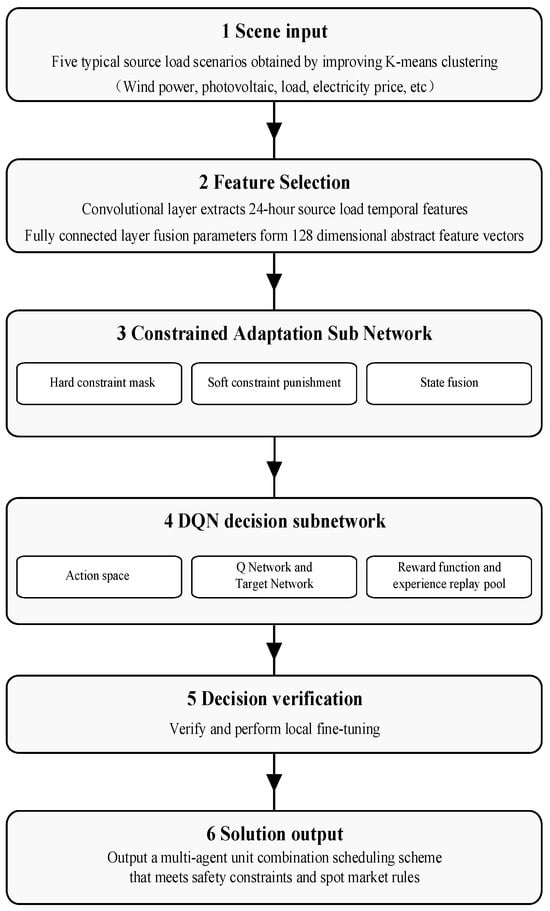
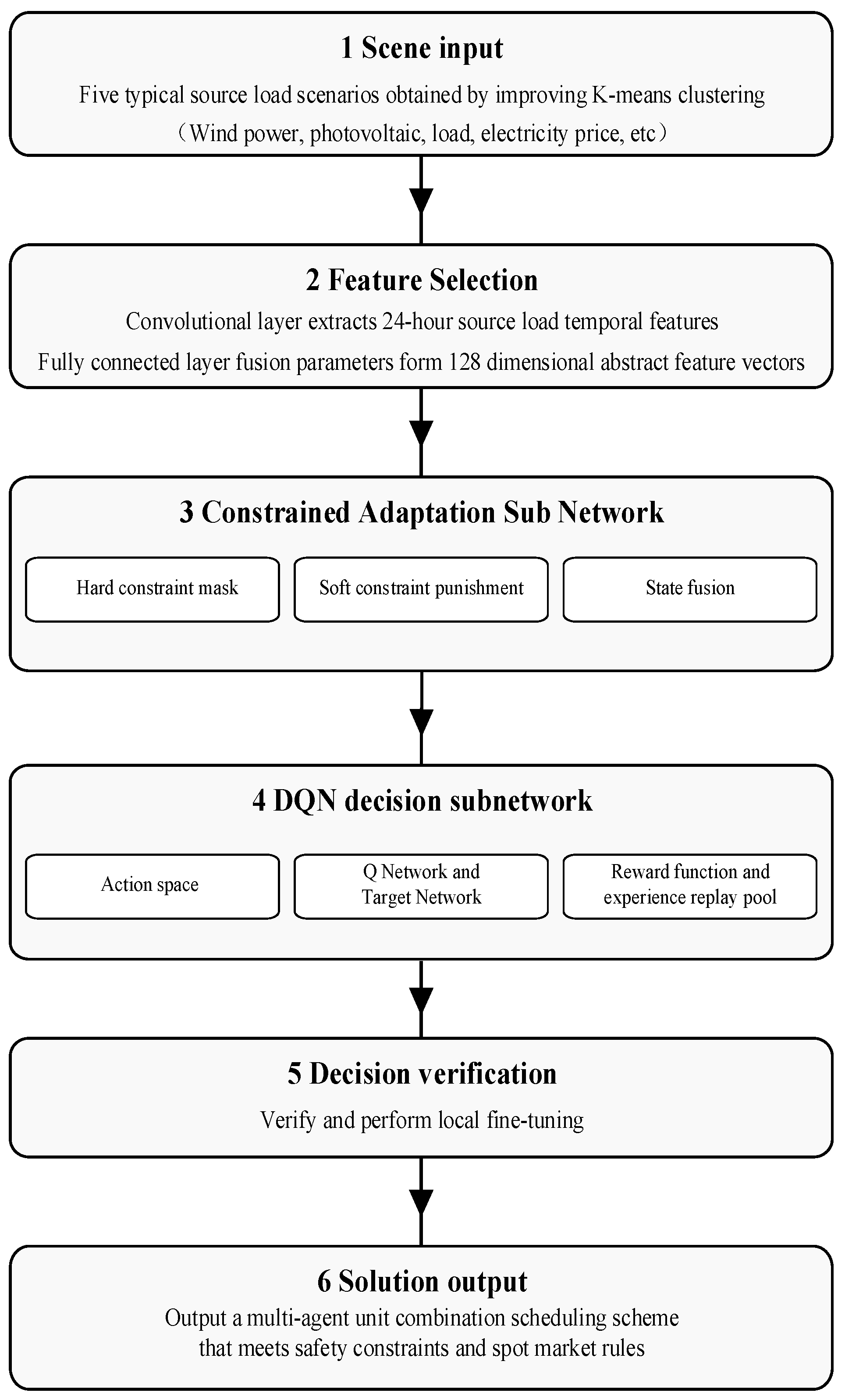
The solution process of the CPNN is highly tailored to the “day-ahead scheduling” process in the electricity market [25]. As depicted in Figure 2, the specific solution process unfolds as follows.
Figure 2.
Solving process of CPNN.
5.2. Model Training Process
In the DQN optimization stage, the proposed framework handles mixed-integer and continuous scheduling decisions through a discrete action representation combined with constraint adaptation. The on/off states of thermal units and the charging/discharging states of energy storage systems are modeled as binary actions, while continuous variables, including generation outputs, storage power and demand response quantities, are discretized into a finite number of operating levels by uniformly partitioning their feasible ranges. During decision making, infeasible actions violating hard operational or network constraints are filtered by the hard constraint masking mechanism, and soft constraint violations are penalized in the reward function. In addition, a lightweight feasibility adjustment is applied to project the selected action onto the nearest admissible operating point when necessary, thereby ensuring feasibility and acceptable solution accuracy in the mixed-integer scheduling problem.
5.2.1. Pre-Training Phase
The goal of the preliminary training is to assist the feature extraction subnetwork and the constraint adaptation subnetwork in acquiring knowledge. The intention is to enable these subnetworks to understand the fundamental characteristics and constraint rules of the power system [26]. This objective is accomplished by utilizing measured data from the electricity market, which includes 2000 sets of offline optimal solutions for UC problems, as the training set.
- Dataset construction: The input consists of load scene data from the source and subject parameter data. These data are labeled with abstract feature vectors and constraint compliance information corresponding to offline optimal solutions.
- Loss function: In this paper, it is proposed to employ the mean square error loss function to enhance the accuracy of feature extraction and constraint adaptation during the optimization process.
Among them, is the number of samples. is the abstract feature vector of the optimal solution. is the average constraint violation degree, and is the penalty weight.
- 3.
- Following a series of 1000 iterations with the Adam optimizer, the loss value is recorded as less than 10−3. This outcome marks the conclusion of the preliminary training stage.
5.2.2. DQN Optimization Stage
During the optimization stage of the DQN, the emphasis is placed on cultivating dynamic decision-making capabilities within the framework of reinforcement learning. The primary objective is to learn UC strategies that maximize social welfare through trial-and-error approaches [27].
- 1.
- -greedy strategy: The initial exploration probability is set to 0.9, which undergoes a decay of 0.05 with every 100 iterations, eventually reaching a value of 0.1. This adjustment is made to achieve a balance between “action exploration” and “optimal utilization”.
- 2.
- Sample collection: It is possible to execute action in the source–load scene, thus resulting in the immediate acquisition of rewards and the subsequent transition to state . The final stage of the process is the storage of the sample in the experience replay pool.
- 3.
- Q-network update: Gradient descent can be employed to minimize the time difference error.Among them, takes 256 as the batch size, and is the target Q-value.
- 4.
- Convergence judgment: If the fluctuation in the mean reward over 5000 consecutive steps is less than 0.1%, it is determined that the model training has converged, and the iteration process is terminated. In this study, the maximum number of training episodes is set to 1000, while the above convergence criterion is used as an early-stopping condition.
6. Example Analysis
To validate the effectiveness of the constructed “Intelligent Decision Model for UC Adapted to Multi-Agent Collaboration in the Electricity Market” in real-world distribution network scenarios, this paper selects the typical IEEE 33-node distribution system as the test case. Based on this, a variety of entities, such as traditional thermal power plants, RE stations, independent ES systems, and VPP, are incorporated to create a simulation environment that conforms to the operational mechanism of the electricity market and the interactive characteristics of multiple entities. The scheduling cycle is configured as 24 h with a time resolution of 1 h.
6.1. Parameter Settings
To enable the testing system to accurately characterize the scenario of “multi-agent collaboration in distribution networks”, this study proposes an extension to the original IEEE 33-node system. Specifically, this extension includes targeted connection of peak-shaving thermal power units at nodes 3 and 6; installation of wind farms at node 17 and photovoltaic power stations at node 21; deployment of an independent ES system at node 12; and aggregation of some industrial and commercial loads at nodes 8–10 into a VPP. This configuration is capable of comprehensively reflecting the collaborative regulation mechanism among multiple entities on the source side (including thermal power, wind power, and photovoltaic power), the ES system side, and the load side within the electricity market environment.
- 1.
- Parameters of thermal power unitsAs the primary controllable resource of the system, the output range, climbing ability, and start–stop characteristics of thermal power units directly affect the system’s peak shaving ability and operational economy. The parameters of thermal power units are shown in Table 1.Table 1. Parameters of thermal power units.
- 2.
- Wind farm parametersThe wind farm is connected to node 17, and its output is determined by wind speed, which follows a Weibull distribution. The wind power parameters are delineated in Table 2.Table 2. Wind farm parameters.
- 3.
- Photovoltaic power station parametersThe photovoltaic is connected to node 21, which experiences optimal irradiation conditions at typical distribution network locations. The illumination intensity is modeled using a beta distribution. The parameters of light intensity are delineated in Table 3.Table 3. Light intensity parameters.
- 4.
- Load model parametersThe IEEE 33-node load comprises three distinct components: residential, industrial, and commercial. Residential loads are characterized by rigidity, whereas industrial and commercial loads are more amenable to adjustment. The proportions of load composition and prediction error are shown in Table 4.Table 4. Load model parameters.
- 5.
- ES system parametersThe ES system is connected to node 12, which has the capacity to engage in energy arbitrage, in addition to its utilization for load regulation and backup services. The ES system parameters are delineated in Table 5.Table 5. ES system parameters.
- 6.
- VPP parametersIn order to simulate the process of demand response entities participating in market regulation, the industrial and commercial loads at nodes 8, 9, and 10 are aggregated to form a VPP. The precise parameters are delineated in Table 6.Table 6. VPP parameters.
6.2. Visualization of CPNN Solution Process
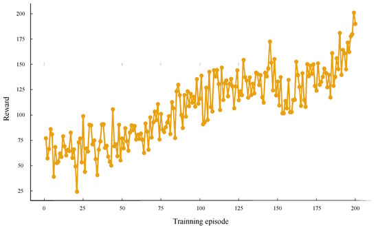
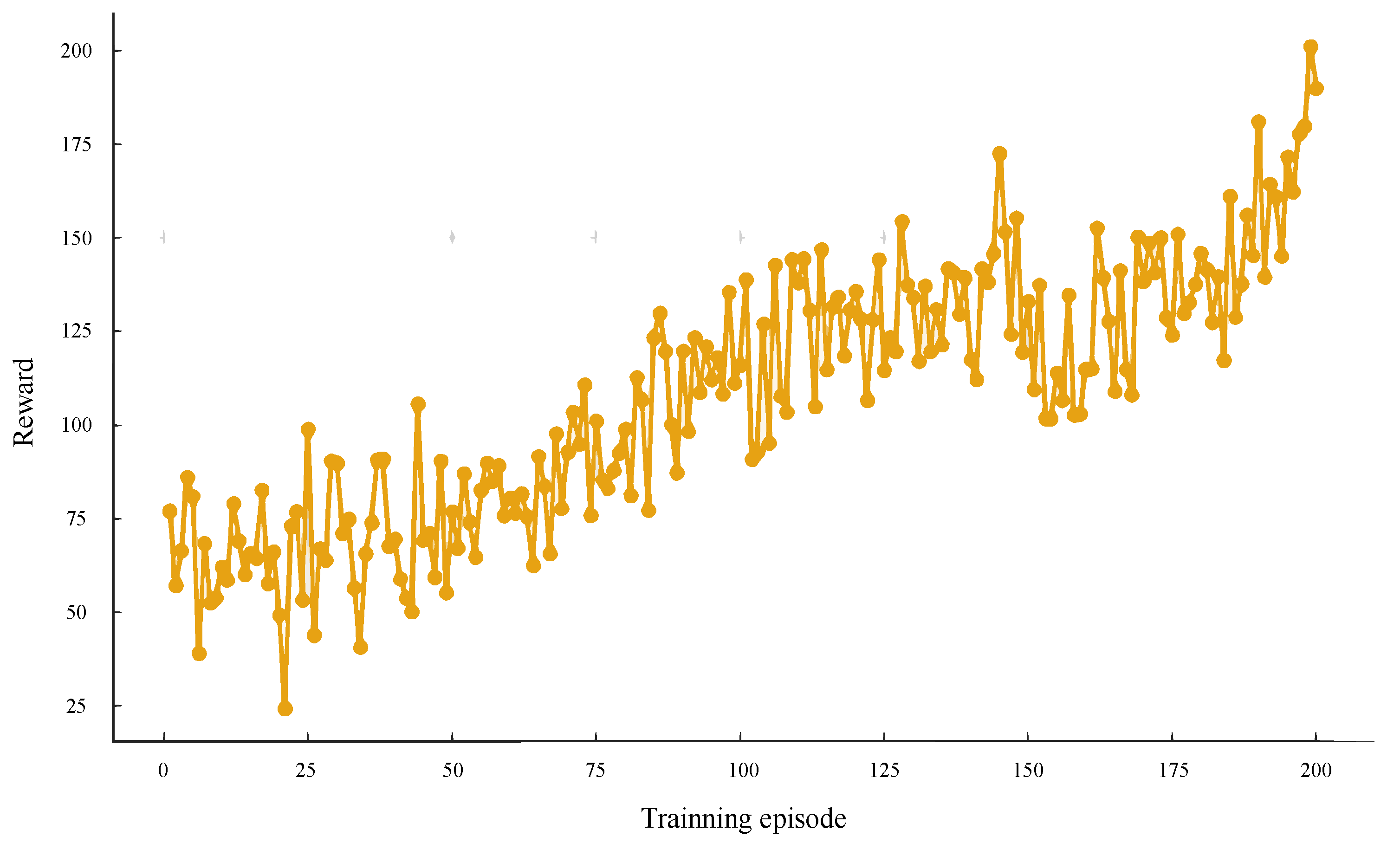
The cumulative reward changes of the network during the training process are illustrated in Figure 3, where the maximum number of training episodes is set to 1000, and an early-stopping mechanism is adopted. The fluctuation in reward values in the early stages of training is indicative of the randomness of the strategy network during the exploration phase. Conversely, as the number of training iterations increases, the reward value gradually rises and converges to a stable range in the middle and later stages. This is an indication that the network has successfully learned a scheduling strategy that combines economy and feasibility.
Figure 3.
Reward curve during neural network training process (maximum 1000 episodes with early stopping).
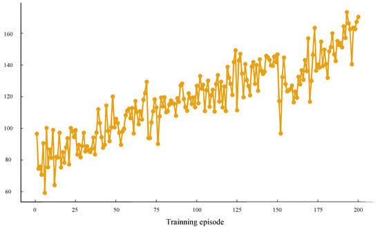
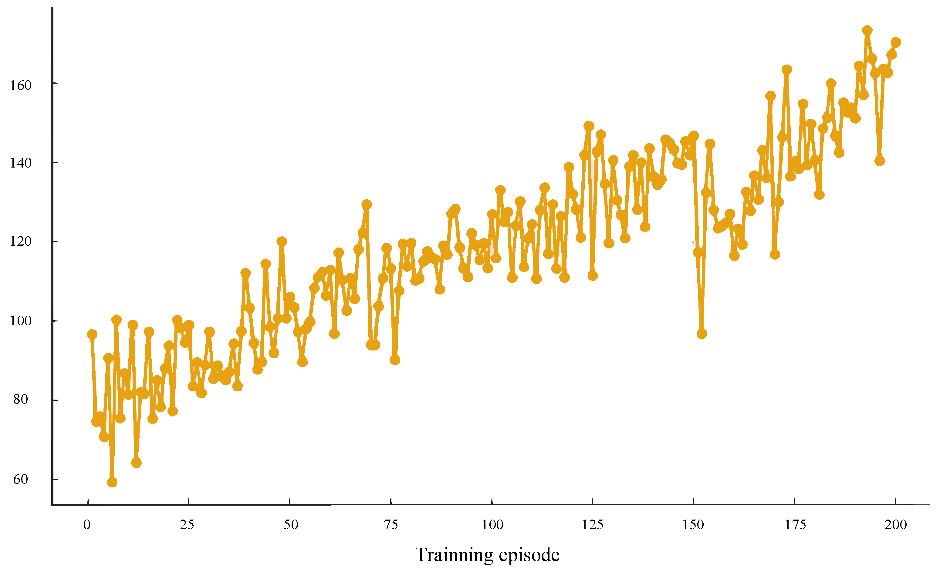
As demonstrated in Figure 4, the Q-value of the primary network undergoes fluctuations in accordance with the number of training iterations. The maximum number of training episodes is set to 1000, and training is terminated early once the convergence criterion is satisfied. The Q-value demonstrates significant fluctuations in the initial 100 iterations, subsequently converging gradually, suggesting that the value function has approached a state of stability. This network is capable of accurately evaluating the value of different actions in the current state.
Figure 4.
Q-value of the main network versus training iteration curve (maximum 1000 episodes with early stopping).
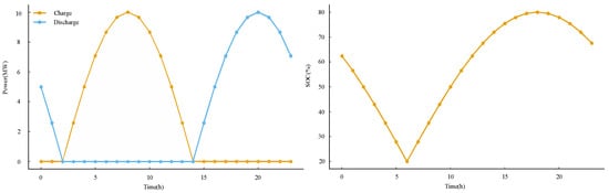
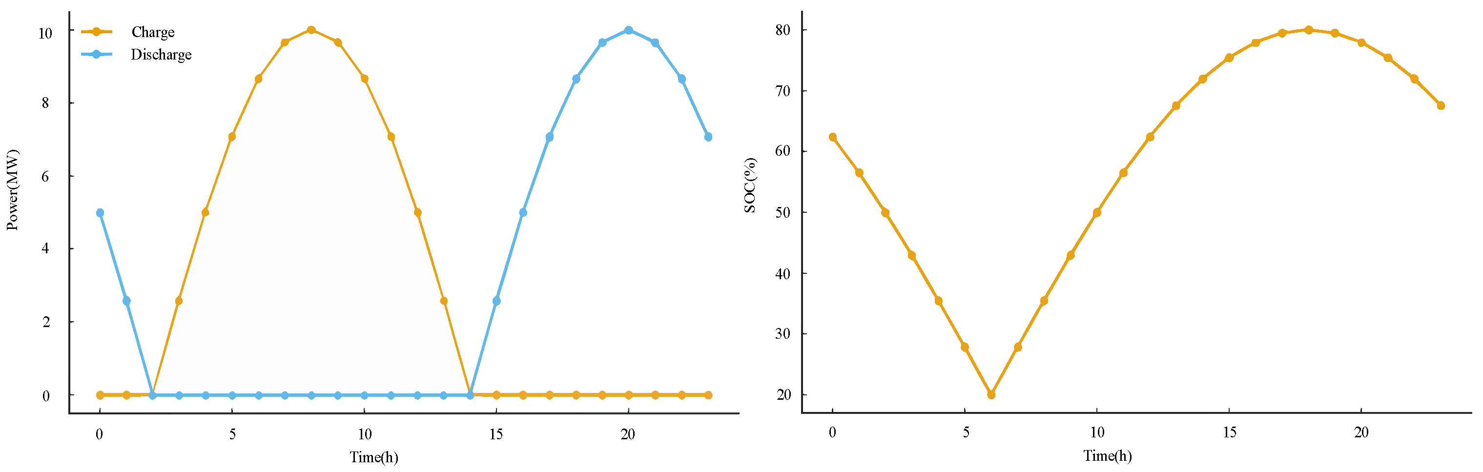
As demonstrated in Figure 5, the SOC and charge–discharge behavior of the ES system on typical days can be observed. SOC varies within the constraint range of 20% to 80%, exhibiting a distinct “low valley charging, high peak discharging” characteristic. The charging and discharging power curve is smooth and conforms to the operational constraints of the equipment, reflecting the network’s ability to learn the physical characteristics of ES and use them for peak shaving and valley filling.
Figure 5.
SOC and charge–discharge behavior of ES system.
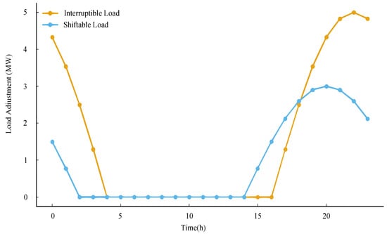
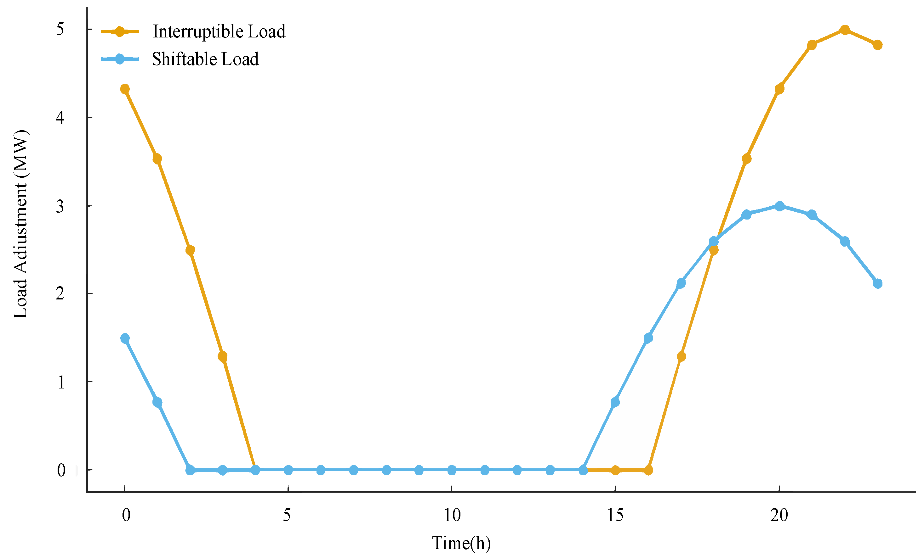
As illustrated in Figure 6, the response behavior of interrupted loads and transferable loads in a VPP is demonstrated. The response is primarily observed during the evening peak load period, where interrupted loads exhibit a rapid reduction effect, while transferable loads adjust in time before and after the peak period. The findings suggest that neural networks possess the capacity to effectively utilize the adjustability of industrial and commercial loads, thereby enhancing system operation without compromising the overall power balance.
Figure 6.
Response behavior of interrupted loads and transferable loads in VPPs.
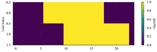
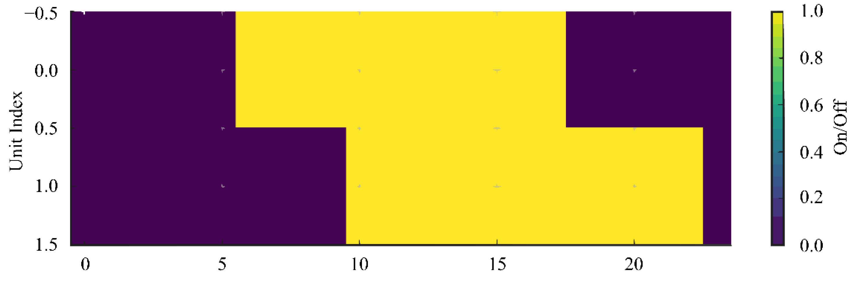
Figure 7 presents the start–stop status of two thermal power units in a typical day, expressed as a heat map. It is evident that the number of unit starts and stops is relatively limited, and the continuity of the operating range is satisfactory, indicating that the neural network strategy can effectively circumvent the additional costs engendered by frequent starts and stops, and exhibits commendable scheduling smoothness.
Figure 7.
Start–stop status of thermal power units on typical days.
6.3. Analysis of Example Results
In order to verify the advantages of the proposed CPNN model in UC and multi-agent collaborative scheduling, this section selects mixed-integer linear programming (MILP) and a genetic algorithm (GA) as comparative benchmarks and evaluates them in terms of three aspects: operational characteristics, economy, and robustness.
6.3.1. Comparison of Scheduling Effectiveness and Operational Characteristics
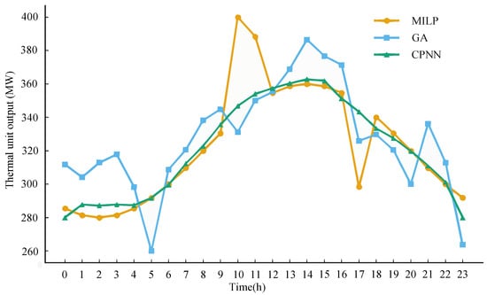
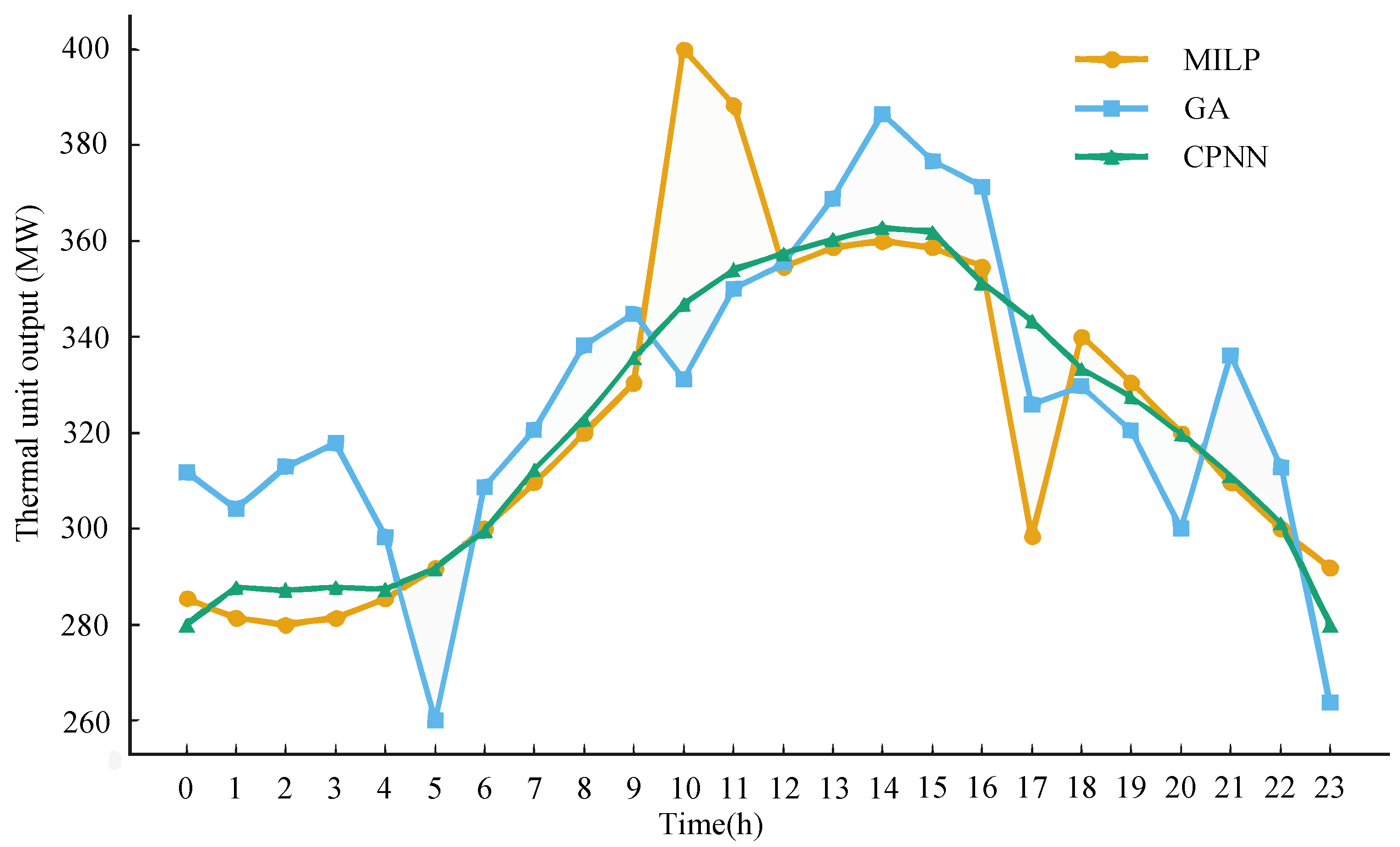
The MILP scheme strictly satisfies power balance and unit constraints in each time period. However, it has been demonstrated that output changes are more “sharp” during load mutation periods. Furthermore, the GA curve fluctuates greatly, with some periods approaching the upper or lower limit of output. In comparison, the overall output trajectory of CPNN is smoother, with natural transitions between peaks and valleys. It has also been demonstrated that no violations occurred throughout the entire period, thus demonstrating good feasibility and scheduling flexibility. As illustrated in Figure 8, the output curves of thermal power units have been obtained by three different algorithms.
Figure 8.
Comparison of output curves of thermal power units obtained by three algorithms.
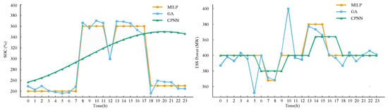
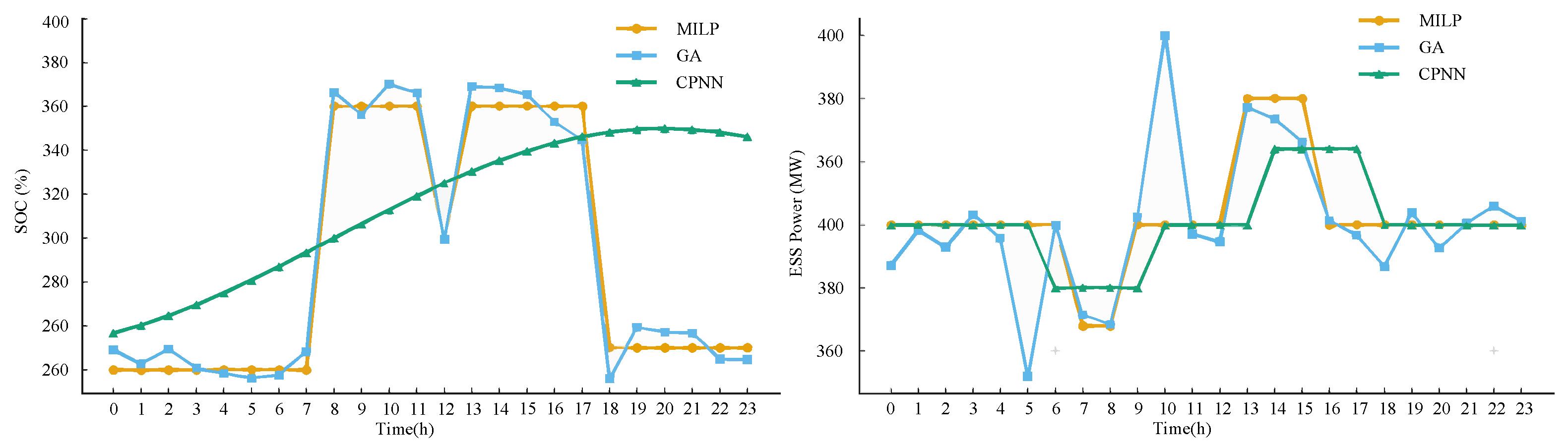
The SOC of MILP exhibits a distinct segmented pattern, characterized by “edge-to-edge operation” that frequently occurs near the upper and lower limits. The SOC of GA surpasses the upper limit of 80% in certain periods, thereby incurring a risk of exceeding the designated threshold. Conversely, the SOC curve of CPNN maintains stability within the range of 20% to 80%, exhibiting a consistent and continuous trajectory by charging during low valley periods and discharging during peak periods. The leftmost figure in Figure 9 provides a comparison of the changes in ES SOC obtained by three algorithms. The corresponding charge and discharge power curves are shown on the right of Figure 9. It is evident that the charge and discharge operations of CPNN exhibit greater uniformity, thereby circumventing the occurrence of short-term high-power charge and discharge in the MILZ scheme. This advantageous characteristic is conducive to prolonging the ES life.
Figure 9.
Energy storage SOC changes and corresponding charge–discharge power curves obtained by three algorithms.
6.3.2. Comparison of Economic Indicators
The following section will present a comparative analysis of the mean daily total operating costs and social welfare under the three algorithms demonstrated in Table 7. It is evident that MILP exhibits the lowest operating cost and the highest social welfare, a consequence of its capacity to ascertain the global optimal or approximate global optimal solution. The total cost of CPNN is marginally higher than that of MILP, yet significantly lower than that of GA, with the corresponding social welfare approximating that of MILP. Conversely, GA is influenced by random search and local convergence, resulting in the highest total cost and the lowest social welfare.
Table 7.
Typical daily total operating costs and social welfare under three algorithms.
6.3.3. CPNN Robustness Analysis
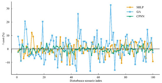
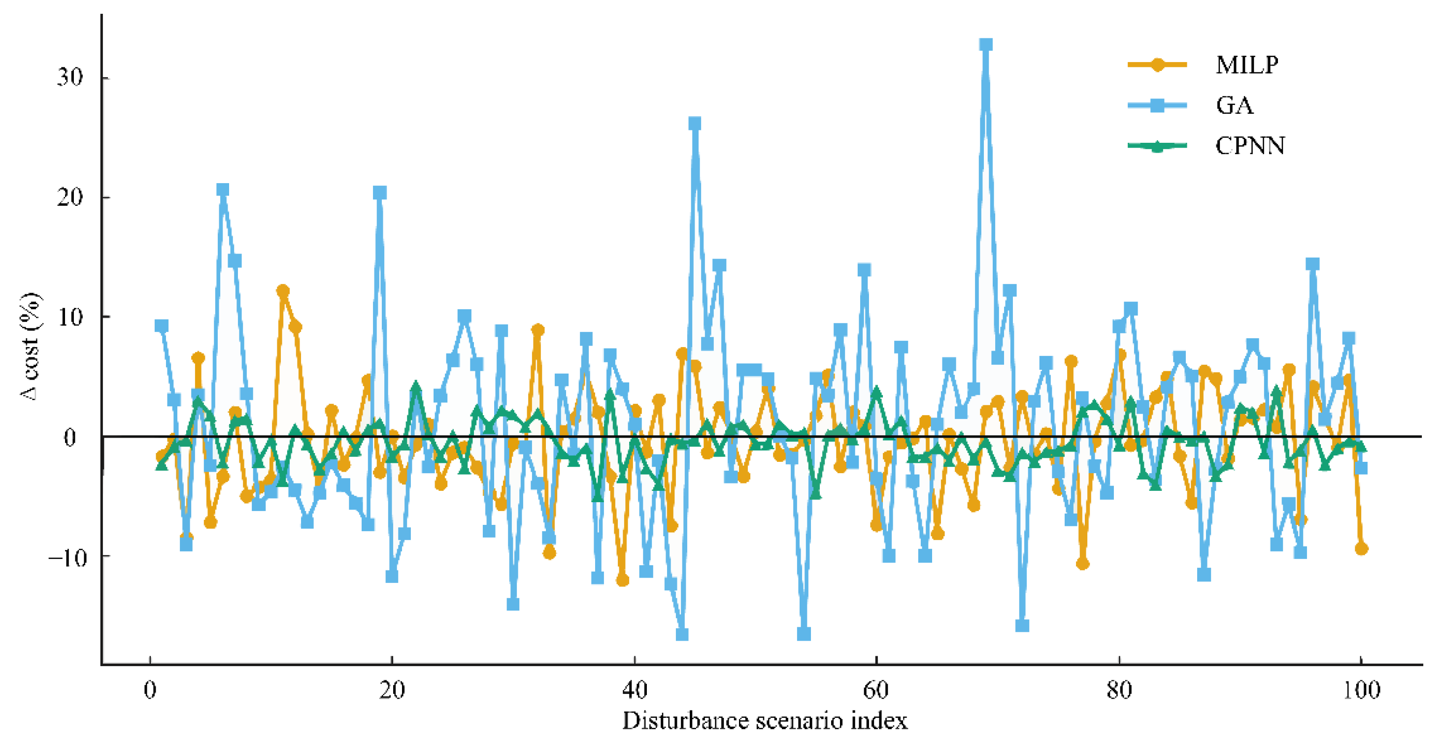
In order to evaluate the adaptability of three algorithms under source–load uncertainty disturbance, this paper constructed a random disturbance scenario of wind and photovoltaic output ±20% and load ±5% outside the benchmark scenario. The cost offset distribution and feasible solution ratio of the algorithms are presented in Figure 10. The results demonstrate that CPNN exhibits a 100% feasible solution ratio across all disturbance scenarios. The cost offset is observed to be concentrated within a narrow range of ±5%. MILP is found to be susceptible to failure or prolonged execution under extreme disturbances, resulting in a marginally lower proportion of feasible solutions. Conversely, GA demonstrates the lowest feasible solution ratio, and the cost offset box exhibits a wider distribution, exhibiting heightened sensitivity to source–load wave motion. Overall, ANN has been shown to exhibit superior robustness to fluctuations in wind and solar power output and load forecasting errors, while ensuring the feasibility of the solution. The system is particularly well-suited to scenarios that demand rapid response, such as rolling optimization and real-time scheduling.
Figure 10.
Adaptability of three algorithms under source–load uncertainty disturbance.
6.4. Statistical Performance Evaluation Under Multiple Scenarios
To further verify the generalization capability of the proposed CPNN scheduling method, a batch evaluation is conducted under multiple source–load scenarios generated by the improved K-means clustering method. All reduced typical scenarios are considered, and MILP, GA and CPNN are tested under identical system settings with a 24 h scheduling horizon. The statistical results are summarized using four metrics, namely, the average total operating cost, the average social welfare, the feasible solution ratio, and the average computation time, in order to comprehensively evaluate the economic performance, solution reliability and computational efficiency of the proposed method under multi-scenario conditions.
As shown in Table 8, MILP achieves the best economic performance but requires the longest computation time, while GA exhibits inferior economic performance and a lower feasible solution ratio. In contrast, the proposed CPNN obtains competitive operating cost and social welfare with a much shorter computation time and the highest feasible solution ratio, demonstrating its effectiveness and suitability for fast multi-scenario scheduling in the electricity market.
Table 8.
Statistical comparison of three algorithms under multiple scenarios.
7. Conclusions
The CPNN model proposed in this article has demonstrated significant advantages in the domain of multi-agent collaborative UC scheduling. A comparison of CPNN with MILP and GA demonstrates that it exhibits a satisfactory balance with regard to scheduling effectiveness, operational characteristics and economy. In circumstances involving source–load uncertainty, CPNN has been shown to exhibit enhanced robustness and greater adaptability. These properties contribute to the system’s feasibility and the effective scheduling of resources in the face of substantial fluctuations in RE output and load prediction errors. The system is well-suited to real-time scheduling scenarios, characterized by the need for rapid response. Consequently, CPNN provides an intelligent and efficient solution for multi-agent collaborative scheduling in the electricity market. Nevertheless, it is worth noting that the CPNN, as a deep learning-driven framework, inherently has limitations: it relies on large-scale high-quality labeled data for model training, and its internal decision-making logic lacks sufficient interpretability. Future research will focus on addressing these issues, such as integrating few-shot learning to reduce data dependence and introducing attention mechanisms to improve model interpretability, thereby further promoting its practical application in complex power systems.
Author Contributions
Conceptualization and methodology, X.Z. and C.L.; writing—review and editing, N.Y. and J.H.; methodology, data curation, and writing—original draft preparation, P.L., Z.L. and X.C.; supervision, Z.L. All authors have read and agreed to the published version of the manuscript.
Funding
The authors gratefully acknowledge financial support from the State Grid Shandong Electric Power Company’s Scientific and Technological Project (Grant No. 52062625000D).
Data Availability Statement
The original contributions presented in this study are included in this article. Further inquiries can be directed to the corresponding author.
Conflicts of Interest
The authors declare no conflicts of interest. The authors declare that this study received funding from the State Grid Shandong Electric Power Company’s Scientific and Technological Project. The funder was not involved in the study design, collection, analysis, interpretation of data, the writing of this article, or the decision to submit it for publication.
References
- Deng, X.; Lv, T. Power system planning with increasing variable renewable energy: A review of optimization models. J. Clean. Prod. 2020, 246, 118962. [Google Scholar] [CrossRef] [Scilit]
- Zhou, Y.; Han, Z.; Zhai, Q.; Wu, L.; Cao, X.; Guan, X. A Data-and-Model-Driven Acceleration Approach for Large-Scale Network-Constrained Unit Commitment Problem with Uncertainty. IEEE Trans. Sustain. Energy 2025, 16, 2299–2311. [Google Scholar] [CrossRef] [Scilit]
- Ajagekar, A.; You, F. Deep reinforcement learning based unit commitment scheduling under load and wind power uncertainty. IEEE Trans. Sustain. Energy 2022, 14, 803–812. [Google Scholar] [CrossRef] [Scilit]
- Yang, H.; Liang, R.; Zheng, Y.; Peng, S.; Rae, A.; Ackom, E.; Johnston, A.J. Receding horizon optimization of power demand response for production-oriented users with real-time operating status-awareness. IEEE Trans. Consum. Electron. 2025; early access. [CrossRef] [Scilit]
- Xiong, H.; Shi, Y.; Chen, Z.; Guo, C.; Ding, Y. Multi-stage robust dynamic unit commitment based on pre-extended-fast robust dual dynamic programming. IEEE Trans. Power Syst. 2022, 38, 2411–2422. [Google Scholar] [CrossRef] [Scilit]
- Shi, Z.; Xu, Y.; Wang, Y.; He, J.; Li, G.; Liu, Z. Coordinating multiple resources for emergency frequency control in the energy receiving-end power system with HVDCs. IEEE Trans. Power Syst. 2022, 38, 4708–4723. [Google Scholar] [CrossRef] [Scilit]
- Bajpai, P.; Dash, V. Hybrid renewable energy systems for power generation in stand-alone applications: A review. Renew. Sustain. Energy Rev. 2012, 16, 2926–2939. [Google Scholar] [CrossRef] [Scilit]
- Li, P.; Song, L.; Qu, J.; Huang, Y.; Wu, X.; Lu, X.; Xia, S. A two-stage distributionally robust optimization model for wind farms and storage units jointly operated power systems. IEEE Access 2021, 9, 111132–111142. [Google Scholar] [CrossRef] [Scilit]
- Weng, Y.; Geng, G.; Jiang, Q. Unit commitment of power systems considering system inertia constraints and uncertainties. IET Renew. Power Gener. 2024, 18, 2512–2523. [Google Scholar] [CrossRef] [Scilit]
- Li, R.; Yang, Y. Multi-objective capacity optimization of a hybrid energy system in two-stage stochastic programming framework. Energy Rep. 2021, 7, 1837–1846. [Google Scholar] [CrossRef] [Scilit]
- Li, J.; Wang, T.; Tang, S.; Jiang, J.; Chen, S. Planning distribution network using the multi-agent game and distribution system operators. Front. Energy Res. 2023, 11, 1244394. [Google Scholar] [CrossRef] [Scilit]
- Li, Z.; Li, H.; Zhang, M.; Xu, B.; Chu, H.; Ni, S.; Guo, L. A coordinated source-network expansion planning framework for incremental distribution grid based on non-cooperative game theory. Energy Rep. 2025, 13, 5616–5627. [Google Scholar] [CrossRef] [Scilit]
- Shao, C.; Qian, T.; Wang, Y.; Wang, X. Coordinated planning of extreme fast charging stations and power distribution networks considering on-site storage. IEEE Trans. Intell. Transp. Syst. 2020, 22, 493–504. [Google Scholar] [CrossRef] [Scilit]
- Kazemtarghi, A.; Mallik, A.; Chen, Y. Dynamic pricing strategy for electric vehicle charging stations to distribute the congestion and maximize the revenue. Int. J. Electr. Power Energy Syst. 2024, 158, 109946. [Google Scholar] [CrossRef] [Scilit]
- Yao, C.; Chen, S.; Salazar, M.; Yang, Z. Joint routing and charging problem of electric vehicles with incentive-aware customers considering spatio-temporal charging prices. IEEE Trans. Intell. Transp. Syst. 2023, 24, 12215–12226. [Google Scholar] [CrossRef] [Scilit]
- Zhu, J.; Zeng, K.; Chen, J.; Zhao, W.; Liu, W.; Zhu, W. Transfer-Based Approximate Dynamic Programming for Rolling Security-Constrained Unit Commitment with Uncertainties. Prot. Control. Mod. Power Syst. 2024, 9, 42–53. [Google Scholar] [CrossRef] [Scilit]
- Wang, L.; An, X.; Xu, H.; Zhang, Y. Multi-agent-based collaborative regulation optimization for microgrid economic dispatch under a time-based price mechanism. Electr. Power Syst. Res. 2022, 213, 108760. [Google Scholar] [CrossRef] [Scilit]
- Liu, Y.; Li, Y.; Hou, G.; Qin, H. Multi-Objective Short-Term Operation of Hydro-Wind-Photovoltaic-Thermal Hybrid System Considering Power Peak Shaving, the Economy and the Environment. Energies 2024, 17, 4698. [Google Scholar] [CrossRef] [Scilit]
- Bessa, R.; Moreira, C.; Silva, B.; Matos, M. Handling renewable energy variability and uncertainty in power system operation. In Advances in Energy Systems: The Large-Scale Renewable Energy Integration Challenge; Wiley: Hoboken, NJ, USA, 2019; pp. 1–26. [Google Scholar] [CrossRef] [Scilit]
- Ziane, A.; Necaibia, A.; Sahouane, N.; Dabou, R.; Mostefaoui, M.; Bouraiou, A.; Khelifi, S.; Rouabhia, A.; Blal, M. Photovoltaic output power performance assessment and forecasting: Impact of meteorological variables. Sol. Energy 2021, 220, 745–757. [Google Scholar] [CrossRef] [Scilit]
- Lv, S.; Li, J.; Guo, Y.; Shi, Z. A typical distributed generation scenario reduction method based on an improved clustering algorithm. Appl. Sci. 2019, 9, 4262. [Google Scholar] [CrossRef] [Scilit]
- De, G.; Wang, X.; Tian, X.; Xu, T.; Tan, Z. A collaborative optimization model for integrated energy system considering multi-load demand response. Energies 2022, 15, 2033. [Google Scholar] [CrossRef] [Scilit]
- Li, M.; Chen, S.; Shen, Y.; Liu, G.; Tsang, I.W.; Zhang, Y. Online multi-agent forecasting with interpretable collaborative graph neural networks. IEEE Trans. Neural Netw. Learn. Syst. 2022, 35, 4768–4782. [Google Scholar] [CrossRef]
- Lu, X.; Qiu, J.; Zhang, C.; Lei, G.; Zhu, J. Assembly and competition for virtual power plants with multiple ESPs through a “recruitment-participation” approach. IEEE Trans. Power Syst. 2023, 39, 4382–4396. [Google Scholar] [CrossRef] [Scilit]
- Ihlemann, M.A.I.; Delarue, E. A Flexible Open-Source Modelling Framework to Support Decision Making for Future Energy Systems. Ph.D. Thesis, KU Leuven, Leuven, Belgium, 2022. [Google Scholar]
- Sayed, A.R.; Wang, C.; Anis, H.I.; Bi, T. Feasibility constrained online calculation for real-time optimal power flow: A convex constrained deep reinforcement learning approach. IEEE Trans. Power Syst. 2022, 38, 5215–5227. [Google Scholar] [CrossRef] [Scilit]
- Hasan, M.; Lwin, K.; Imani, M.; Shabut, A.; Bittencourt, L.F.; Hossain, M. Dynamic multi-objective optimisation using deep reinforcement learning: Benchmark, algorithm and an application to identify vulnerable zones based on water quality. Eng. Appl. Artif. Intell. 2019, 86, 107–135. [Google Scholar] [CrossRef] [Scilit]

Disclaimer/Publisher’s Note: The statements, opinions and data contained in all publications are solely those of the individual author(s) and contributor(s) and not of MDPI and/or the editor(s). MDPI and/or the editor(s) disclaim responsibility for any injury to people or property resulting from any ideas, methods, instructions or products referred to in the content. |
© 2026 by the authors. Licensee MDPI, Basel, Switzerland. This article is an open access article distributed under the terms and conditions of the Creative Commons Attribution (CC BY) license.