


Abstract
As renewable energy penetration continues to increase, converter control dynamics play a critical role in power system synchronization, making small-signal synchronization stability an important concern in converter-dominated power systems. Grid-following (GFL) and grid-forming (GFM) converters differ in synchronization mechanisms and stability characteristics, and their coordinated operation may introduce complex dynamic interactions. These differences and interactions make it challenging to clarify how converter control dynamics affect synchronization stability, both individually and through their interaction. This paper develops a unified small-signal modeling and path decomposition method (PDM) for GFL and GFM converters in single- and two-converter systems. Based on this, a stability contribution index is introduced to quantify and compare the effect of each path on the dominant oscillatory mode. The proposed method separates the effects of AC network, single converter, and inter-converter interaction paths and reveals how key control parameters affect system stability, thereby providing a theoretical basis for stability assessment and coordinated parameter design in multi-converter systems.
1. Introduction
Driven by global efforts to mitigate climate change, renewable energy sources are being rapidly integrated into power systems, resulting in the large-scale deployment of power electronic devices (PEDs) [1]. Consequently, modern power systems are undergoing a structural transition from conventional power systems dominated by synchronous generators to converter-dominated power systems.
Large-scale integration of PEDs weakens system inertia and damping, which deteriorates dynamic responses and poses severe challenges to power system stability [2]. In 2009, a sub-synchronous oscillation event occurred when two wind farms in Texas, USA, were connected to the grid through series-compensated transmission lines. The oscillation was attributed to the interaction between the series-compensated transmission line and the wind turbine control system, a phenomenon termed sub-synchronous control interaction (SSCI), and resulted in equipment damage [3]. In 2025, two periods of sustained oscillations were observed in the Spain–Portugal power system before the subsequent blackout and were considered contributing factors to the incident [4]. In response to the stability challenges posed by the increasing penetration of PEDs, the power system stability category has been extended to account for their fast dynamics [5].
Against this background, numerous studies have focused on GFL converters because they remain the predominant converter type for renewable energy integration. These converters rely on phase-locked loops (PLLs) for grid synchronization, making PLL dynamics a key factor in their small-signal synchronization stability. Existing studies have shown that PLL dynamics can introduce phase lag and negative damping under weak-grid conditions, thereby increasing the risk of oscillatory instability [6,7]. This vulnerability becomes more pronounced as short-circuit ratios (SCRs) decrease [8]. Reference [9] further indicates that reduced grid strength significantly weakens system stability, particularly when the PLL bandwidth approaches that of the DC-link voltage control (DVC) loop.
To overcome the inherent limitations of GFL under weak grids, GFM converters, which can establish voltage amplitude and frequency without relying on grid-phase tracking, have attracted considerable attention. Among the available GFM control strategies, virtual synchronous generator (VSG) control that emulates the rotor dynamics of synchronous machines is a representative and widely adopted approach [10,11]. Reference [12] developed a small-signal model of GFM converter and used frequency-domain analysis to examine the effects of key VSG parameters on small-signal synchronization stability. Reference [13] proposed a distributed parameter design method for the power loop that considers both stability margin and dynamic performance improvement, providing a basis for VSG parameter optimization. Unlike GFL, GFM may suffer reduced stability under strong-grid conditions, as shown through eigenvalue analysis in Reference [14]. Reference [15] further investigated “anomalous stiff-grid instability” and identified the interaction between the Terminal Voltage Control (TVC) loop and the Power Synchronization Control (PSC) loop as the main cause of instability through participation factor analysis. More recently, reference [16] proposed controller voltage feedback-based PSC to improve GFM stability under wide SCR variations, including suppression of low-frequency resonance in stiff grids.
Although single-converter analysis reveals the stability characteristics of different converter types, practical power systems usually involve multiple devices operating cooperatively. Interactions between GFL and GFM may introduce more complex small-signal synchronization stability problems. Reference [17] used μ-analysis to examine the effects of different converters on GFL, showing that parallel GFL–GFM operation enhances stability, with stronger enhancement at shorter distances, whereas parallel operation of two GFL units reduces stability more strongly as their distance decreases. Reference [18] studied how the GFL–GFM capacity ratio affects equivalent grid strength and thus small-signal synchronization stability, providing guidance for GFM capacity allocation. Reference [19] used phasor-domain models and eigenvalue analysis to assess mixed GFL–GFM systems in multi-bus networks. Reference [20] reduced large systems to stability-equivalent two-machine subsystems while retaining converter–converter and converter–network interactions. Reference [21] established a hybrid converter state space model including GFM and GFL and quantitatively studied the effects of PLL dynamics, line impedance, and GFM inertia and damping on stability using eigenvalue analysis. Reference [22] also used eigenvalue analysis to examine parameter effects and participation factors to investigate interactions among devices and between devices and the grid. Reference [23] quantified converter interactions using impedance and eigenvalue impedance ratios, examining control mode and placement effects.
Overall, existing studies have the following limitations: (1) The respective contributions of the AC network and converter control dynamics to their synchronization stability are not always explicitly distinguished. (2) For mixed GFL–GFM systems, the effects of the two converters and their mutual interactions are difficult to distinguish, particularly when assessing their influence on each other’s synchronization stability. (3) Eigenvalue, participation factor, and impedance analyses can assess stability and identify dominant modes but cannot explicitly extract interaction paths or quantify their damping contributions. Thus, the origins, interaction paths, and dominant mechanisms of negative damping remain unclear.
To address the above limitations, this paper proposes a unified small-signal modeling and path decomposition analysis method to systematically reveal the small-signal synchronization stability mechanisms and coupling characteristics of GFL and GFM in single-converter and two-converter scenarios, providing a theoretical basis for stability assessment and parameter optimization of multi-converter systems.
The main contributions of this paper are as follows. First, with a path-based stability contribution index, R, introduced to quantify the effects of corresponding paths, a unified path decomposition method is established to compare the small-signal synchronization characteristics of GFL and GFM converters. Second, the method is extended to a GFL-GFM two-converter system, in which the AC network, single-converter and inter-converter coupling effects are explicitly separated and their R-contributions quantified. This formulation reveals the direction and relative strength of the mutual interactions and provides a structured basis for multi-converter stability analysis and coordinated design.
The remainder of this paper is organized as follows. Section 2 briefly introduces the control structures of GFL and GFM converters and presents their linearized models in the single-converter scenario. Section 3 analyzes the small-signal synchronization stability of the two types of converters in the single-converter scenario and provides a comparative analysis. Section 4 analyzes the small-signal synchronization stability of the GFL–GFM two-converter infinite bus system by separately examining the GFL and GFM synchronization loops and investigates the effects of key controller parameters on system stability. Section 5 discusses the limitations, and Section 6 presents the conclusions and summarizes the contributions of this paper.
2. Modeling of GFL and GFM Converters
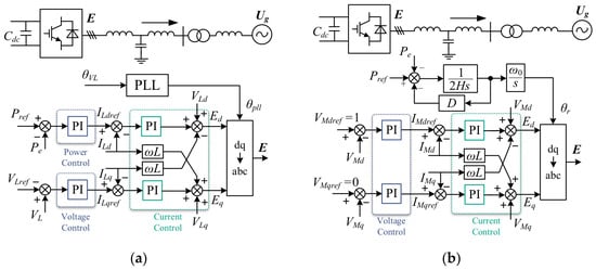
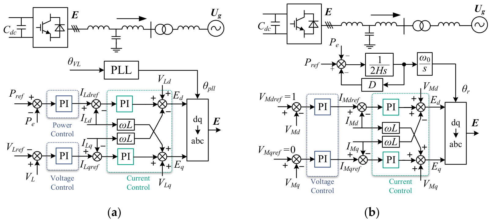
The single-converter infinite bus systems of the grid-following and grid-forming converters are shown in Figure 1. Their main circuit parts are similar, with each converter connected to an infinite bus through an LCL filter and transmission line. The difference lies in the control. GFL adopts power and voltage outer loops and an inner current loop. It relies on the PLL to track the grid phase, with its synchronization dynamics governed by the phase-locking error. In contrast, GFM adopts dq-axis voltage and current dual-loop control. It utilizes PSC control to emulate the rotor motion.
Figure 1.
Single-converter infinite bus system. (a) GFL; (b) GFM.
Small-signal synchronization stability usually involves only slower electromechanical timescales or the DC-link voltage timescale. On this timescale, the fast response of the current loop enables the current to track its reference value almost instantaneously. Therefore, in the subsequent analysis, the dynamics of the AC network and the current loop are neglected. It is assumed that the outer control loops directly control the filter inductor current of the converter and both GFL and GFM can be equivalently represented as current sources. Based on this, linearized models of the two types of converters can be established. A comparison with a detailed time-domain model is provided in Figure A1 (Appendix B) to validate these simplifications.
For the GFL converter, the linearized equations of the AC network and control loops are given as follows [24,25]:
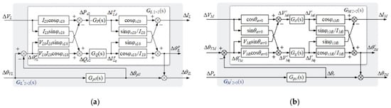
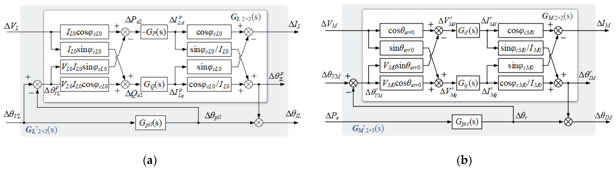
where φcL0 is the steady-state power-factor angle of GFL. The superscript p denotes a physical quantity in the PLL reference frame. is the phase-locking error, which is also equal to the phase of the terminal voltage VL in the PLL reference frame. Since θIL = θpll + , ∆θIL = ∆θpll + ∆. Combining the above equations gives the linearized model of GFL, as shown in Figure 2a. The part outside the synchronization loop PLL can be simply represented by a 2 × 2 transfer function matrix GL. As shown in Figure 2a, the input and output of GL are [∆VL, ∆]T and [∆IL, ∆]T, respectively. The overall model with PLL considered can be represented by GL’, which is also a 2 × 2 transfer function matrix, whose input and output are [∆VL, ∆θVL]T and [∆IL, ∆θIL]T, respectively.
Figure 2.
Linearized model of single-converter infinite bus system. (a) Linearized model of GFL; (b) linearized model of GFM.
The synchronization loop of GFM with VSG control is given by:
Linearizing the above equation gives:
Linearizing the equations related to TVC dynamics gives:
The linearization process for the relevant physical quantities of the terminal voltage VM and the filter inductor current IM in the PSC reference frame is similar to that of GFL. Thus, the linearized model of GFM is obtained, as shown in Figure 2b, where the superscript r denotes a physical quantity in the PSC reference frame. Similar to GFL, the part other than the synchronization loop PSC can also be simply represented by a 2 × 2 transfer function matrix GM, whose input and output are [∆VM, ∆]T and [∆IM, ∆θrJM]T, respectively. And the part with PSC can be represented by a 2 × 3 matrix GM’, whose input and output are [∆VM, ∆θVM, ∆Pe]T and [∆IM, ∆θIM]T, respectively.
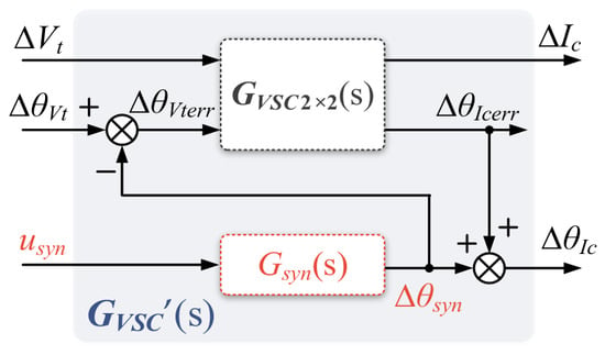
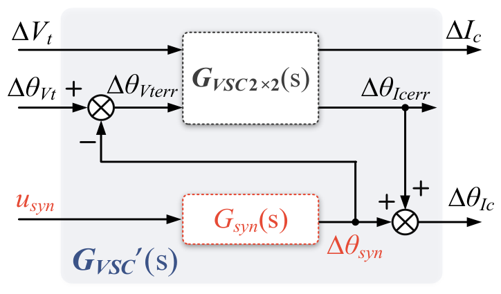
Despite their different synchronization mechanisms, the linearized models of GFL and GFM can be represented by a common closed-loop structure, as shown in Figure 3 [24]. In both cases, the transfer function of the synchronization loop, i.e., Gsyn, determines the converter angle: Gsyn = Gpll for GFL and Gsyn = Gpsc for GFM. The input and output of Gsyn are usyn and θsyn: [usyn, θsyn]T = [∆θVL, ∆θpll]T for GFL and [usyn, θsyn]T = [∆Pe, ∆θr]T for GFM. The remaining control dynamics are collected into a two-dimensional transfer function matrix GVSC: GVSC = GL for GFL and GVSC = GM for GFM. Moreover, the overall model withGsyn is collected into GVSC’. This common formulation enables the two converters to be analyzed within a unified framework.
Figure 3.
Common closed-loop structure of two converters.
3. Small-Signal Synchronization Stability Mechanism Analysis of GFL/GFM
To investigate the effects of converter control dynamics on small-signal synchronization stability, this section combines the path decomposition method [26] with the damping torque analysis method [27] for GFL and GFM converters. Using the linearized models established in the previous section, the overall feedback path of each synchronization loop is decomposed into a network-only path and a path involving both the AC network and the converter control loops. Based on these path structures, a path-based stability contribution index, R, is introduced to quantify the stabilizing or destabilizing effects of each path, thereby revealing the small-signal synchronization stability mechanisms of the two types of converters. The effects of key parameters on the R-based stability characteristics are then examined, providing a theoretical basis for parameter design.
3.1. Path Decomposition for Single-Converter Infinite Bus System
The single-converter infinite bus systems of GFL and GFM can both be simplified into the circuit shown in Figure 4, where Ic denotes the converter output current, Vt denotes the terminal voltage, ZCf denotes the impedance of the filter capacitor, ZVSC denotes the export line impedance, Zg denotes the grid-connection line impedance, and Ug denotes the voltage of the infinite bus source, whose magnitude and phase were set to 1.05 pu and 0, respectively. The corresponding parameters are listed in Table A1 and Table A2 in Appendix A.
Figure 4.
Simplified circuit diagram of the single-converter infinite bus system.
Since the dynamics of inductors and capacitors are neglected, the AC network can be represented by purely algebraic equations. According to the superposition theorem, the terminal voltage vector Vt can be expressed as the sum of the voltages produced by the individual action of each source, as follows:
Rewriting Equation (9) in polar form (Equation (A1) in Appendix A.2) yields the partial derivatives of the magnitude and phase of Vt with respect to those of Ic (Equation (A2) in Appendix A.2), where Kxy reflects how a change in x affects a change in y. Although the PLL and PSC use different synchronization inputs, the AC network relationship is common to the two converters.
The input of the GFL synchronization loop PLL is ∆θVL. Taking the outputs of GL, namely ∆IL and ∆θ, as inputs, and taking the input of PLL, ∆θVL, as well as the inputs of GL, ∆VL and ∆, as outputs, the linearized model of the AC network can be described by the following algebraic equations:
where the elements in KnetL3×2 can be found in Appendix A.2.
Following the method in References [24,25], the linearized model of the single-converter infinite bus system shown in Figure 5 can be established. Note that KnetL3×2 is replaced by a 3 × 3 matrix KeqL3×3, which can be expressed by the elements of KnetL3×2, as given by
Figure 5.
Linearized model of the single-converter infinite bus system.
Regarding GFM, the input of the GFM synchronization loop PSC is ∆Pe, which differs from the input ∆θVL of the PLL. According to the power calculation formula, the expression of Pe can be obtained as
Accordingly, KIMPe and KθIMPe can be obtained. The remaining path decomposition process is similar to that of GFL and is not repeated here, as shown in Figure 5.
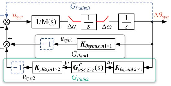
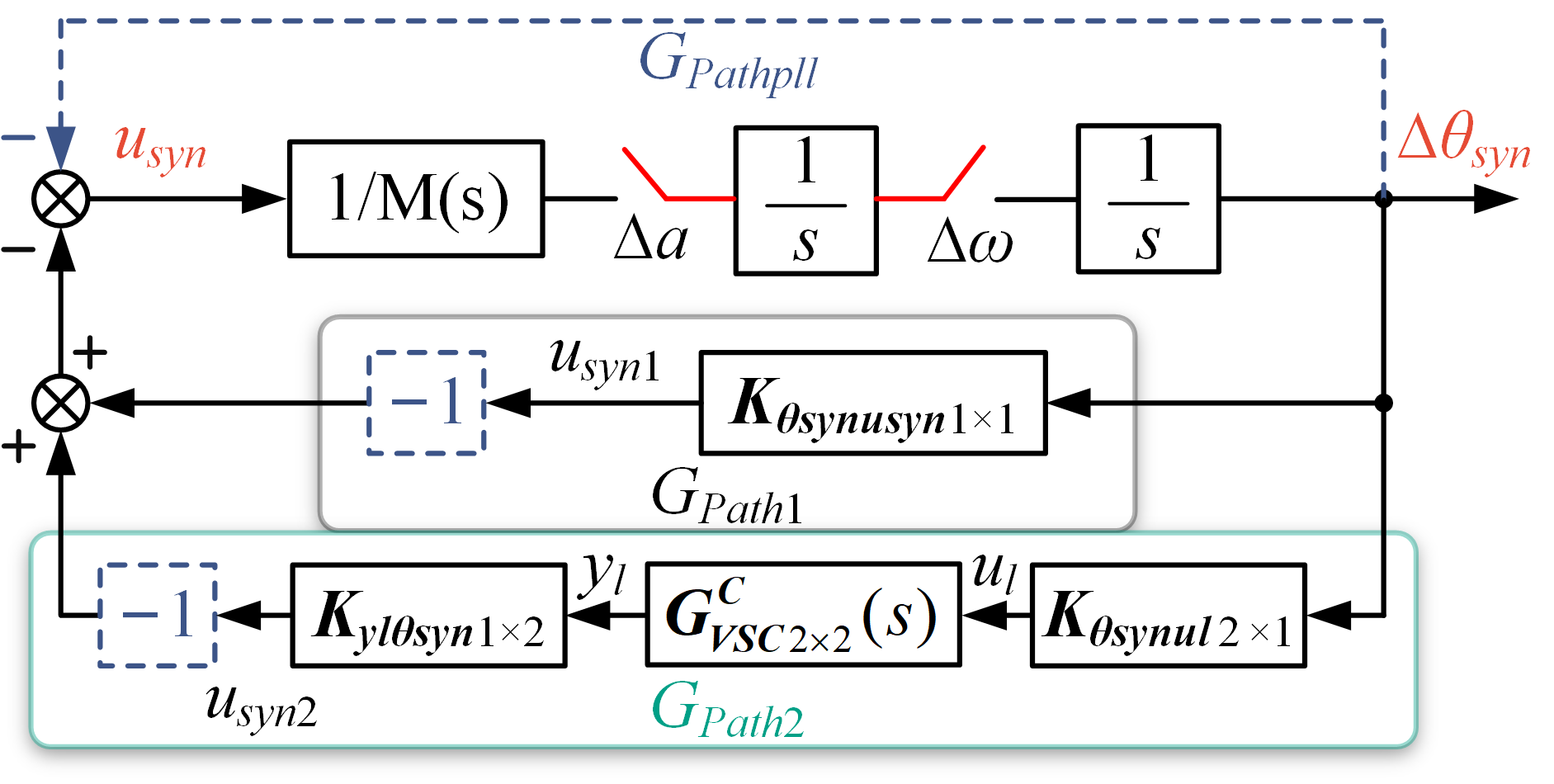
Taking the PLL as the research object, the overall transfer path from ∆θpll to ∆θVL is decomposed into two interaction paths. Path 1 passes only through the AC network. Since the AC network dynamics are neglected, this path is solely determined by the algebraic relationship of the power system network. The terminal voltage phase increment generated by this path is in phase with the PLL phase increment. Path 2 passes through both the AC network and the GFL control loops and therefore captures how the DVC and TVC dynamics affect small-signal synchronization stability.
The inputs and outputs of GL are packaged separately as ul = [∆VL, ∆]T and yl = [∆IL, ∆]T. Thus, KeqL3×3 can be partitioned, and Equation (11) can be written as
Therefore, ∆θVL can be expressed as
Accordingly, ∆θVL can be divided into two parts. ∆θVL1 is the terminal voltage phase increment generated by path 1, and thus,
The transfer function of this path is a constant. ∆θVL2 is the terminal voltage phase increment generated by path 2. The derivation process of the transfer function of this path is as follows:
ul can be expressed as
Moreover,
Combining Equation (16) and Equation (17) gives
Thus, the path decomposition diagram from ∆θpll to ∆θVL was obtained, as shown in Figure 6, where M(s) = 1/(kpplls + kipll). Applying the same procedure to the GFM converter yielded the path decomposition diagram with the same structure as that in Figure 6, where M(s) = 2H/ω0 + D/ω0/s. For both converters, 1/M(s) characterizes the dynamic relationship between the input of the synchronization loop and its acceleration, such that (M(s)) admits a physical interpretation analogous to inertia. Although the GFL and GFM converters employ different synchronization variables, the decomposed models in Figure 6 exhibit similar feedback path structures. It should be noted that the path marked with a dashed line is unique to the GFL converter and reflects the inherent unity negative feedback of the PLL. To quantify and compare the stability effects of corresponding paths on a common basis, this paper defines a path-based stability contribution index, denoted by R:
where ωd is the dominant oscillation frequency, which can be obtained through eigenvalue analysis using the Model Linearizer in Simulink (version R2026b).
Figure 6.
Path decomposition diagram of the single-converter infinite bus system.
Specifically, the system model was linearized at the corresponding operating point, and the eigenvalues of the linearized model were calculated. The eigenvalue pair associated with the dominant synchronization oscillation was then identified, and its oscillation frequency was determined from the imaginary part of the eigenvalues, i.e., fd = |Im(λd)|/(2π). The corresponding angular frequency ωd = 2πfd was subsequently used to evaluate the R index. The total Rall index was obtained by algebraically summing all path contributions. In this regard, a similar indicator has previously been used to assess the damping of grid-connected VSCs [28]. The R index is an analytical index rather than a conventional mechanical damping coefficient, but it can characterize the damping of the dominant oscillatory mode under certain conditions (see Appendix C). Specifically, Rall < 0 indicates that the acceleration a decreases as the angular speed ω increases, corresponding to positive damping and stable system operation. A smaller value of Rall indicates stronger positive damping and hence greater system stability. Conversely, Rall > 0 indicates that a increases with ω, which indicates negative damping of the dominant oscillatory mode. The detailed derivation and applicability of the R index are provided in Appendix C.
3.2. Small-Signal Synchronization Stability Mechanism Analysis of GFL
For the GFL converter, the PLL forward channel contains a PI controller, and the branch with kppll also introduces a damping-equivalent contribution [29]. At this point, Rall comprises the contributions associated with Gpath1, Gpath2, and the inherent unity negative feedback of PLL, and the individual path contributions are calculated as follows:
where i = 1, 2, pll. Rall is given by
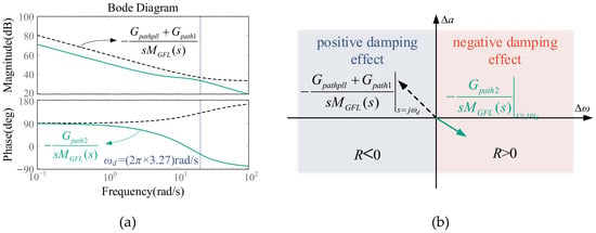
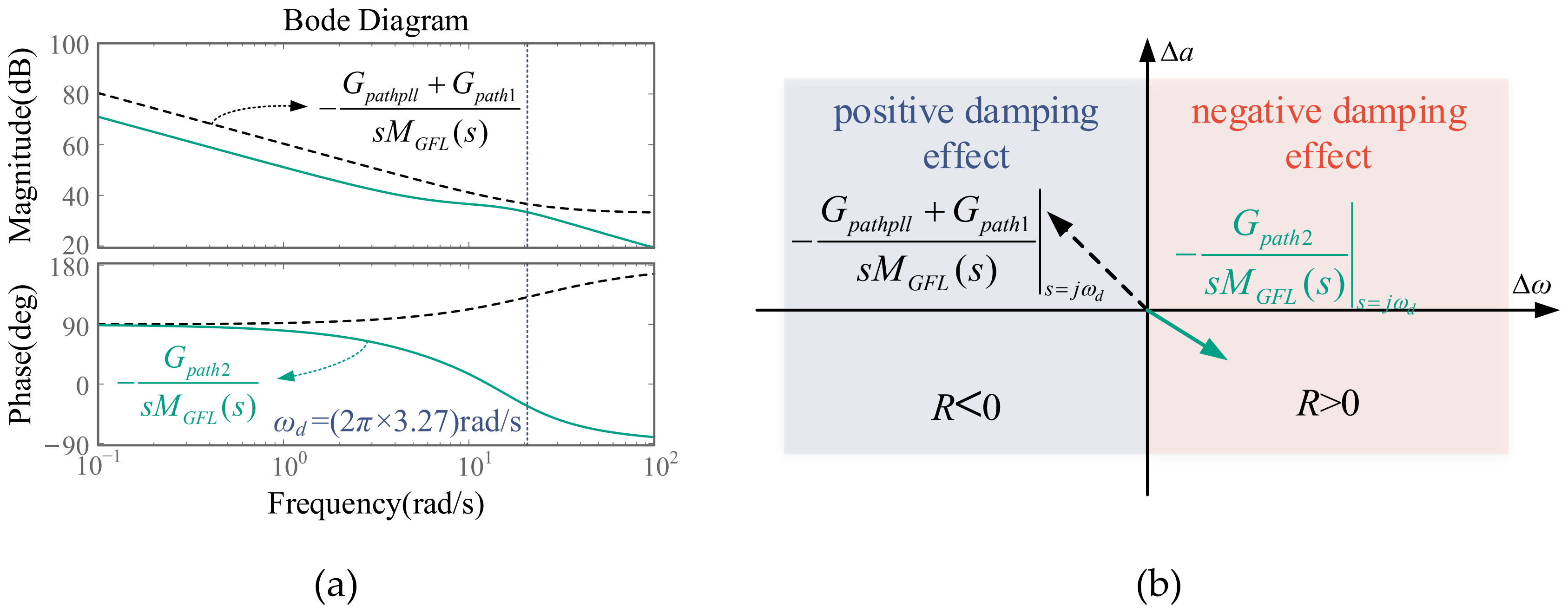
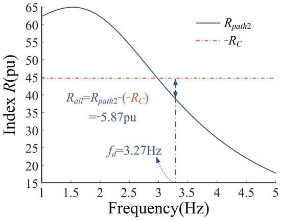
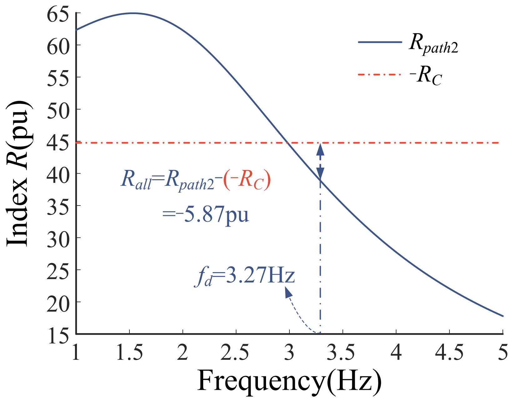
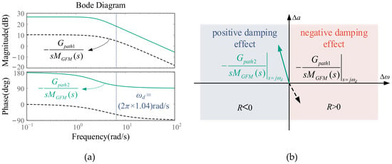
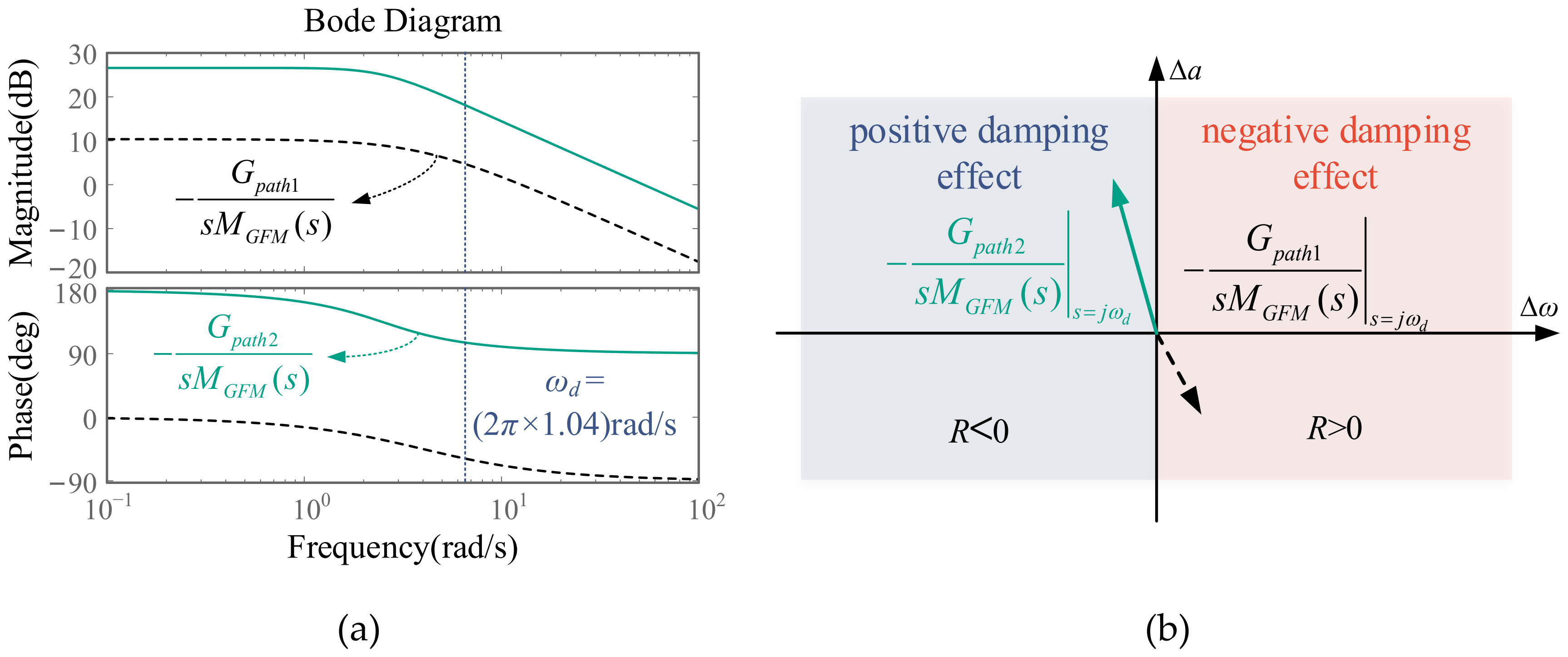
Since both Gpath1 and Gpathpll are constants, the net contributions of the two paths are combined as RC = Rpath1 + Rpathpll. Therefore, the damping contributions to the dominant oscillatory mode can be obtained by comparing Rpath2 and RC at the oscillation frequency ωd. Specifically, Rpathpll is associated with the inherent unity negative feedback of the PLL, whereas Rpath1 is associated with the grid-only path. Rpath2 characterizes the contribution mediated by the DVC and TVC loops to the PLL synchronization dynamics. The Bode plots of the transfer functions associated with each path are shown in Figure 7a, while their respective contributions to acceleration are presented in Figure 7b. The black dashed arrow represents the transfer function associated with Gpath1 + Gpathpll, which introduces acceleration anti-phase with velocity and thereby provides positive damping effect. The green solid arrow represents the transfer function associated with Gpath2, which introduces acceleration in-phase with velocity and thereby provides negative damping effect. As shown in Figure 8, Rpath2 < −RC at the oscillation frequency fd = 3.27 Hz, indicating positive damping of the dominant oscillatory mode.
Figure 7.
Bode plots and damping torque assessment of each path in GFL converter. (a) Bode plots of each path in GFL converter; (b) effects of each path of GFL on acceleration.
Figure 8.
The R index of each path of the GFL-integrated system studied.
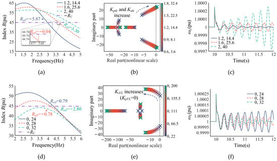
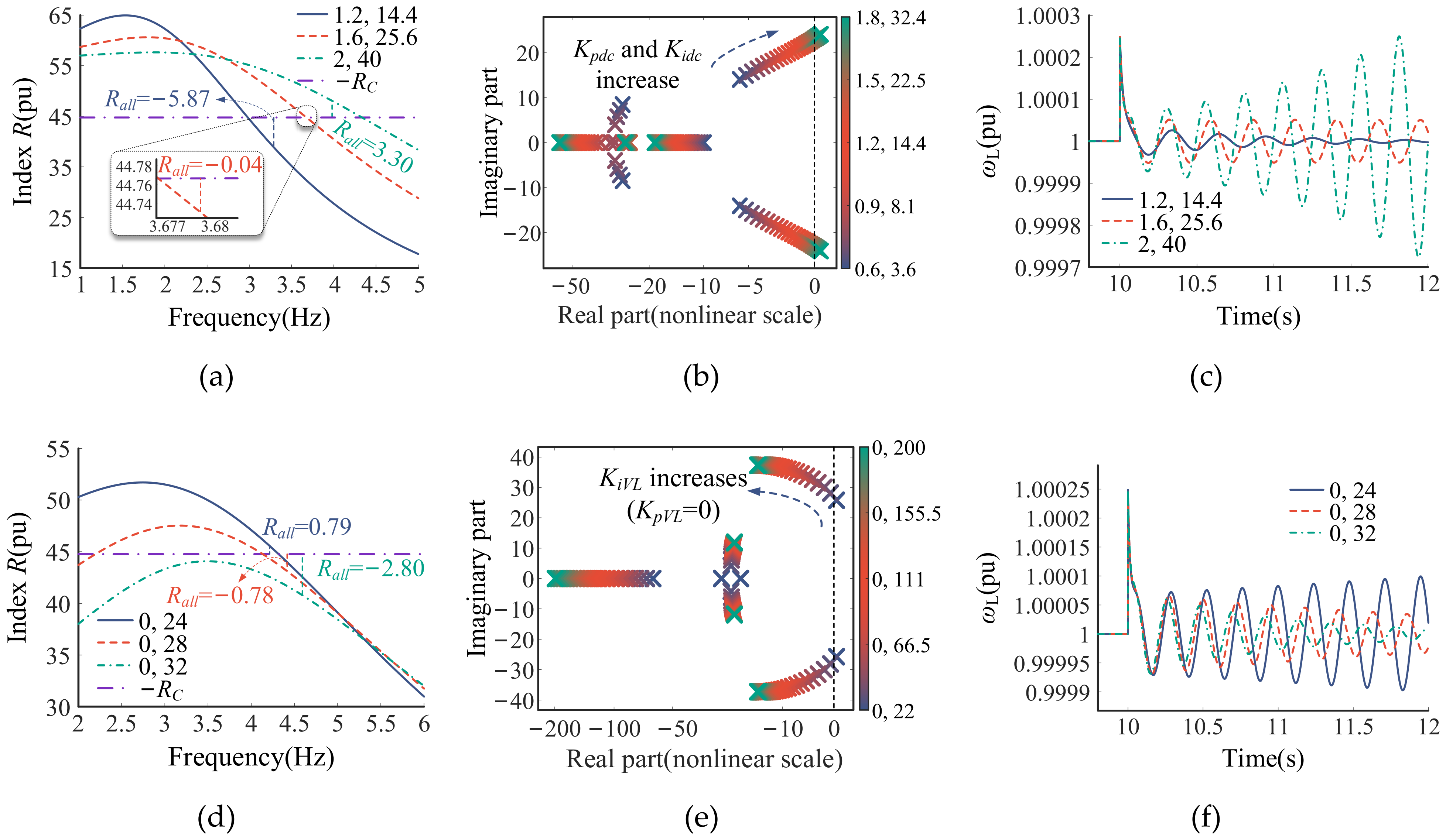
To further analyze the influence of DVC and TVC control parameters on GFL small-signal synchronization stability, the R-based path contributions under different DVC and TVC control parameters are presented in Figure 9a and d, respectively. Each pair of values in the legends represents the proportional and integral gains of the corresponding PI controller.
Figure 9.
R index of each path, root locus and simulation waveforms under different control parameters. (a) R index under different DVC control parameters; (b) root locus under different DVC control parameters; (c) ωL under different DVC control parameters; (d) R index under different TVC control parameters; (e) root locus under different TVC control parameters; (f) ωL under different TVC control parameters.
Since the PLL and network parameters remain unchanged, RC did not vary with the DVC and TVC control parameters; only Rpath2 was affected. For DVC, as shown in Figure 9a, Rpath2 > 0 and provided a destabilizing effect. As Kpdc and Kidc increased, Rpath2 increased, whereas RC changed only slightly with the dominant oscillation frequency changing. Consequently, Rall increased, indicating reduced damping of the dominant oscillatory mode. As shown in Figure 9b, the real parts of the dominant eigenvalues gradually increase and eventually cross the imaginary axis into the right half-plane, indicating a deterioration in system stability with the increase in Kpdc and Kidc. Figure 9c presents the simulation results for validation, where a phase jump disturbance was applied at t = 10 s. It can be seen that the oscillation of ωL after the disturbance decays for (Kpdc, Kidc) = (1.2, 14.4) decayed very slowly for (1.6, 25.6) and grew for (2, 40), which is consistent with the previous analysis. However, further analysis reveals that the effects of the DVC parameters depended on the operating power level of the GFL converter. At relatively high power levels (PL0 = 0.6–1.0 pu), as considered in this paper, increasing the DVC control gains reduced system stability. In contrast, the opposite trend was observed at low power levels (PL0 = 0.1–0.5 pu). The corresponding results are presented in Appendix D. As shown in Figure 9d, Rpath2 decreased while RC changed only slightly with KiVL increasing. Hence, Rall decreased and the stability margin improved. The root locus in Figure 9e and the simulation results in Figure 9f confirm this conclusion.
3.3. Small-Signal Synchronization Stability Mechanism Analysis of GFM
As in the GFL case, RC represents the contribution of the PSC synchronization loop at a given grid strength, excluding the effects of the GFM control-loop dynamics. Rpath2 characterizes the influence of the TVC loop on the PSC synchronization dynamics. As shown in Figure 10b, Gpath1 introduced negative damping to PSC, whereas Gpath2 introduced positive damping to PSC.
Figure 10.
Bode plots and damping torque assessment of each path in GFM converter. (a) Bode plots of each path in GFM converter; (b) effects of each path of GFM on acceleration.
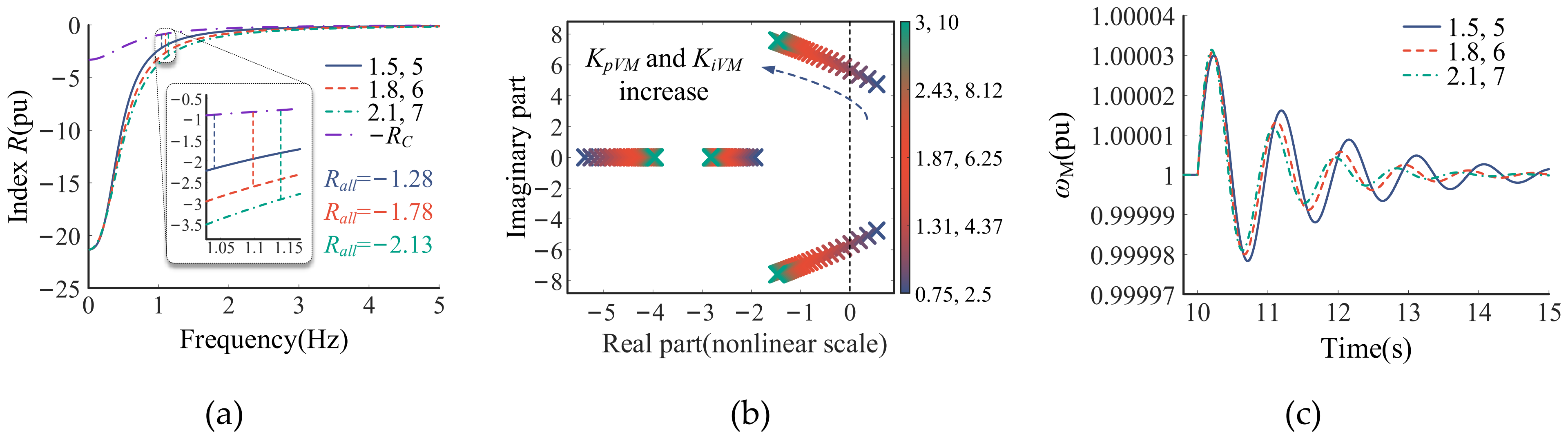
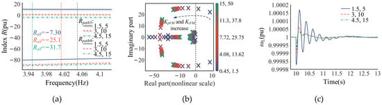
Figure 11 presents the influence of the GFM TVC gains KpVM and KiVM. The R index of each path under different control parameters is shown in Figure 11a. It can be seen that RC is positive, whereas Rpath2 is negative, indicating that the grid is the primary source of destabilizing effects. But −RC is always above Rpath2. Therefore, Rall remains negative, indicating positive damping of the dominant oscillatory mode. When KpVM and KiVM increase, the dominant oscillation frequency increases, Rpath2 decreases, and −RC increases; consequently, Rall decreases, which is beneficial to system stability. The root locus and simulation results in Figure 11b,c further confirm this trend, showing that the dominant eigenvalues move leftward and the oscillations decay more rapidly as KpVM and KiVM increase.
Figure 11.
R index of each path, root locus and simulation waveforms under different control parameters. (a) R index under different TVC control parameters; (b) root locus under different TVC control parameters; (c) ωM under different TVC control parameters.
3.4. Comparison of R-Based Stability Characteristics Between GFL and GFM Under Different Grid Strengths
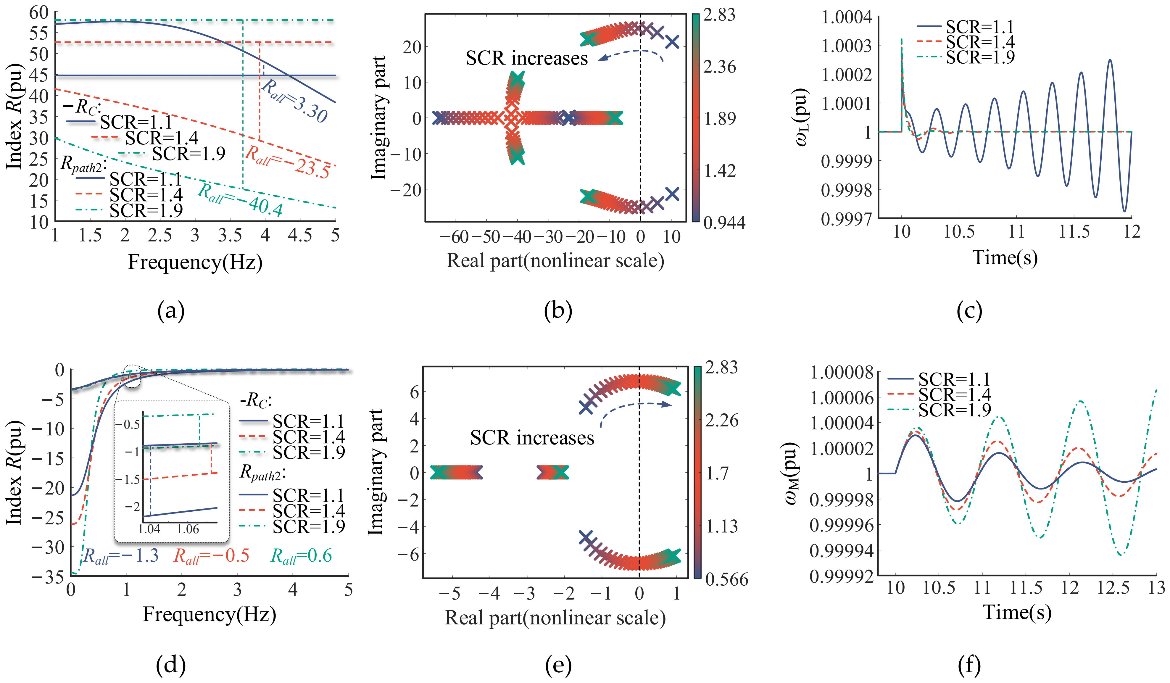
The preceding two subsections investigated the small-signal synchronization stability characteristics of the GFL and GFM converters in single-converter infinite bus systems. Based on these analyses, this subsection compares how their R-based stability characteristics vary with grid strength in a unified analysis framework. As shown in Figure 6, the two converters have analogous path decomposition structures. In both cases, Rall can be decomposed into two components: (1) RC, provided by the synchronization loop itself at a given grid strength; (2) Rpath2, the contribution of the control loop to the synchronization stability of the converter. The variations of these two components over the same range of grid strength are shown in Figure 12a,d.
Figure 12.
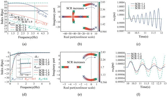
R index, root locus and simulation waveforms under different grid strengths. (a) R index of GFL; (b) root locus of GFL; (c) ωL; (d) R index of GFM; (e) root locus of GFM; (f) ωM.
These results reveal that the GFL and GFM converters exhibited opposite R-based responses to variations in grid strength. For the GFL converter, RC provided a stabilizing effect, whereas Rpath2 provided a destabilizing effect. As the SCR increased, −RC increased and Rpath2 decreased. Consequently, Rall decreased and changed from positive to negative, indicating improved damping of the dominant oscillatory mode of the GFL converter. In contrast, for the GFM converter, RC became destabilizing, whereas Rpath2 became stabilizing and dominated Rall. As the SCR increased, Rpath2 increased, while the smaller variation in RC had a limited effect. Consequently, Rall increased, indicating reduced damping of the dominant oscillatory mode of the GFM converter. Therefore, increasing the SCR decreased Rall for the GFL converter but increased it for the GFM converter. The corresponding root locus results in Figure 12b,e and simulation waveforms in Figure 12c,f confirm these contrasting stability trends.
This section combines the path decomposition method with damping torque analysis to quantify the R-based path contributions to the small-signal synchronization stability of GFL and GFM converters in single-converter infinite bus systems. The parameter analysis shows that increasing the TVC gains decreased Rall and improved the stability of both converters, whereas reducing the DVC gain additionally benefitted the GFL converter in the investigated cases. The comparison further reveals that the negative RC caused by the inherent damping of PLL was the dominant stabilizing effect in the GFL converter, whereas the negative Rpath2 co-determined by outer-loop control and 1/M(s) was the dominant stabilizing effect in the GFM converter. Their opposite Rall responses to grid strength explain why the GFL converter exhibited better stability under strong-grid conditions, whereas the GFM converter exhibited better stability under weak-grid conditions.
4. Small-Signal Synchronization Stability Mechanism Analysis of the GFL–GFM Two-Converter System
In practical power systems, devices rarely operate individually, and the coordinated operation of GFL and GFM devices has been widely applied. To separate single-converter and inter-converter coupling contributions, this section extends the unified path decomposition method to the GFL-GFM two-converter infinite bus system. Based on a linearized model of the system, the interactions between the synchronization loops of the two converters were investigated and the path-specific stability contributions quantified by R, together with the effects of key control parameters, were analyzed.
4.1. Path Decomposition for Two-Converter Infinite Bus System
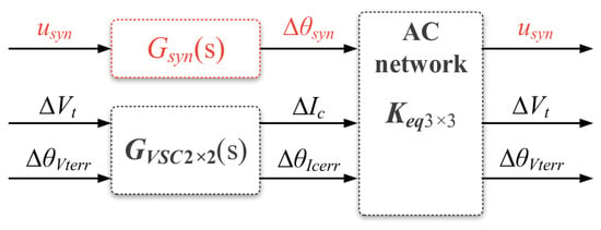
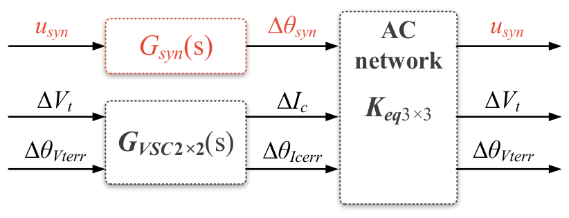
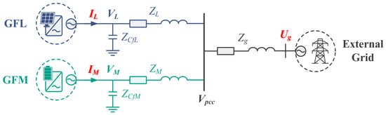
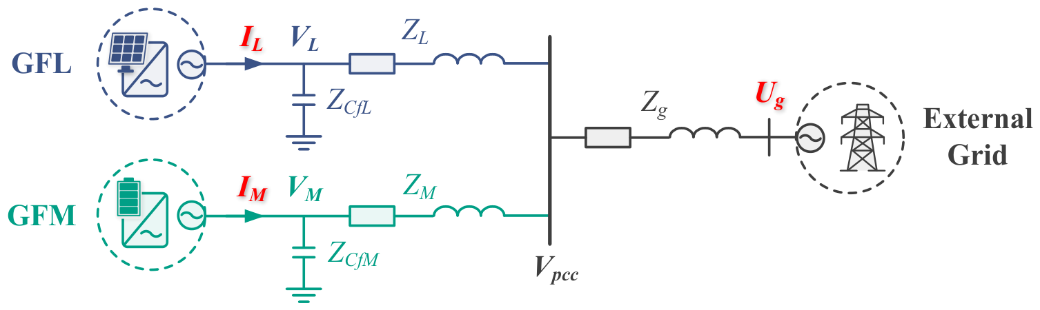
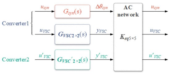
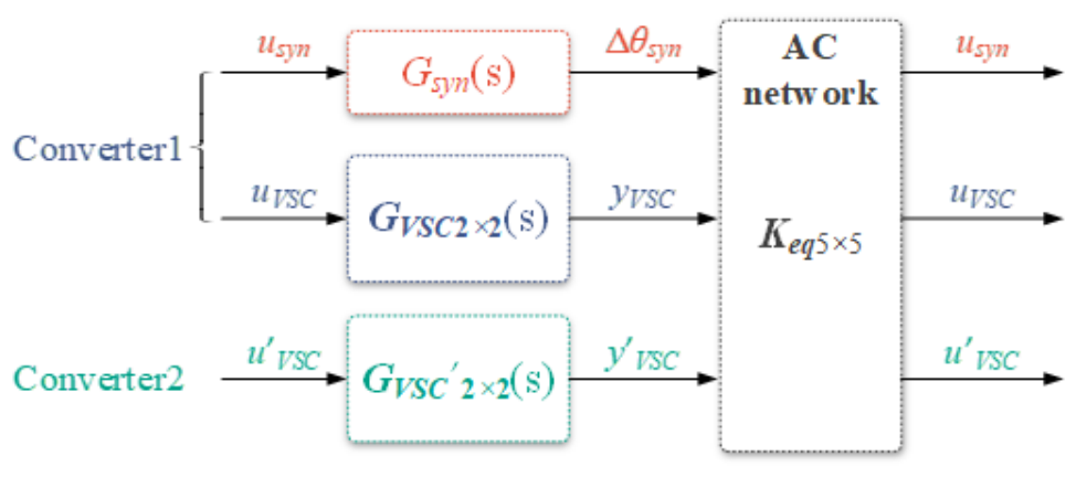
The two-converter infinite bus system containing GFL and GFM can be simplified into the circuit diagram shown in Figure 13. According to the superposition theorem, the terminal voltage vectors VL and VM of the two converters were obtained, and the active power Pe of GFM was then obtained. With reference to the method in the previous section, the matrix Keq5×5 representing the AC network relationship was derived, and the linearized model of the two-converter infinite bus system was obtained, as shown in Figure 14. The parameters of this system are listed in Table A3 in Appendix A.
Figure 13.
Simplified circuit diagram of the two-converter infinite bus system.
Figure 14.
Linearized model of the two-converter infinite bus system.
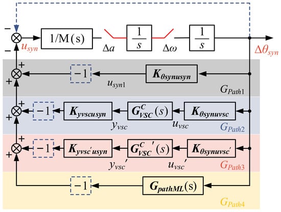
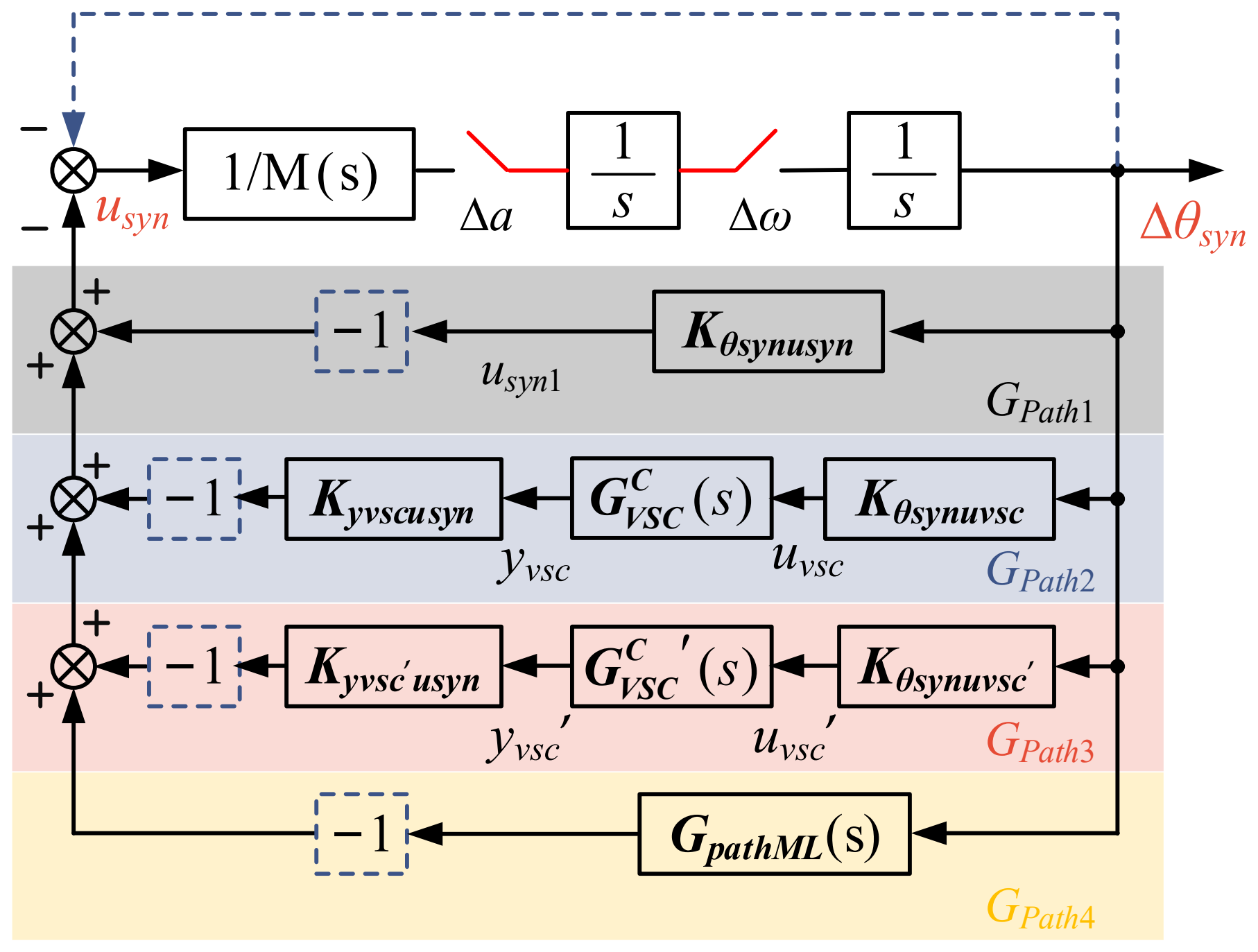
It should be noted that GVSC and GVSC’ represent different converters, with GVSC’ considering the synchronization loop of converter 2. Therefore, the overall transfer path from ∆θsyn to usyn is decomposed into four interaction paths. Path 1 only passes through the AC network, so Gpath1 is a constant. Path 2 passes through the AC network and GVSC of converter 1. Path 3 passes through the AC network and GVSC’ of converter 2, representing the direct stability contribution of converter 2 to the synchronization loop of converter 1. Path 4 simultaneously passes through the AC network, GVSC and GVSC’, reflecting the coupling effect between GFM and GFL.
With PSC as the research object, following the methods in references [24,25], the expressions of paths 2–4 are derived, as given by Equations (A3)–(A5) in Appendix A.2. The resulting path decomposition diagram of the GFL–GFM two-converter infinite bus system is shown in Figure 15.
Figure 15.
Path decomposition diagram of the GFL-GFM two-converter infinite bus system.
4.2. Influence of GFL on the Synchronization Stability of GFM
According to Figure 15, the Rall of the system is given by
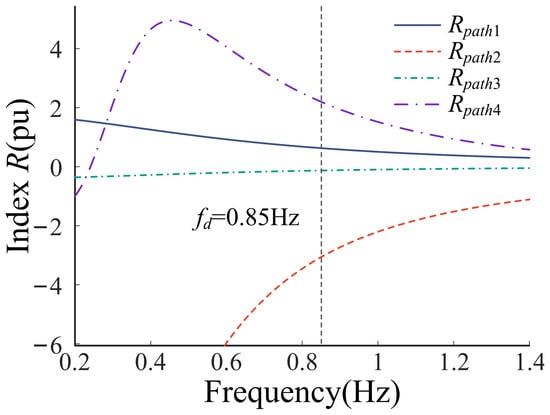
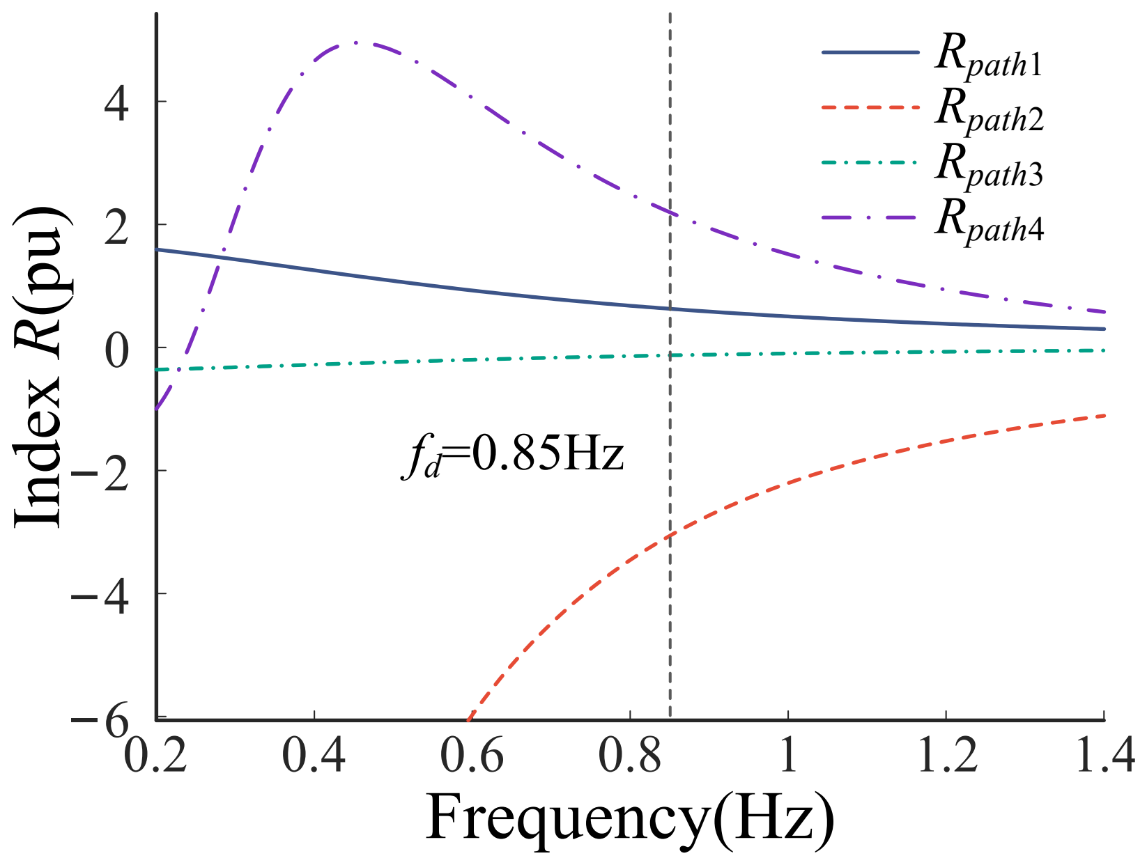
where RC = Rpath1. The R contributions of all paths are shown in Figure 16. At the dominant oscillation frequency, paths 2 and 3 yielded negative R contributions and therefore exerted stabilizing effects, whereas paths 1 and 4 exerted destabilizing effects. These results indicate that the GFL converter improved the synchronization stability of the GFM converter directly through path 3 but deteriorated it indirectly through path 4. Since the positive R contribution of path 4 was greater than the magnitude of the negative R contribution of path 3, the GFL-related paths yielded a net destabilizing effect, mainly associated with the GFL-GFM coupling path.
Figure 16.
R index of each path of the studied system.
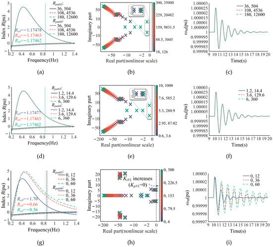
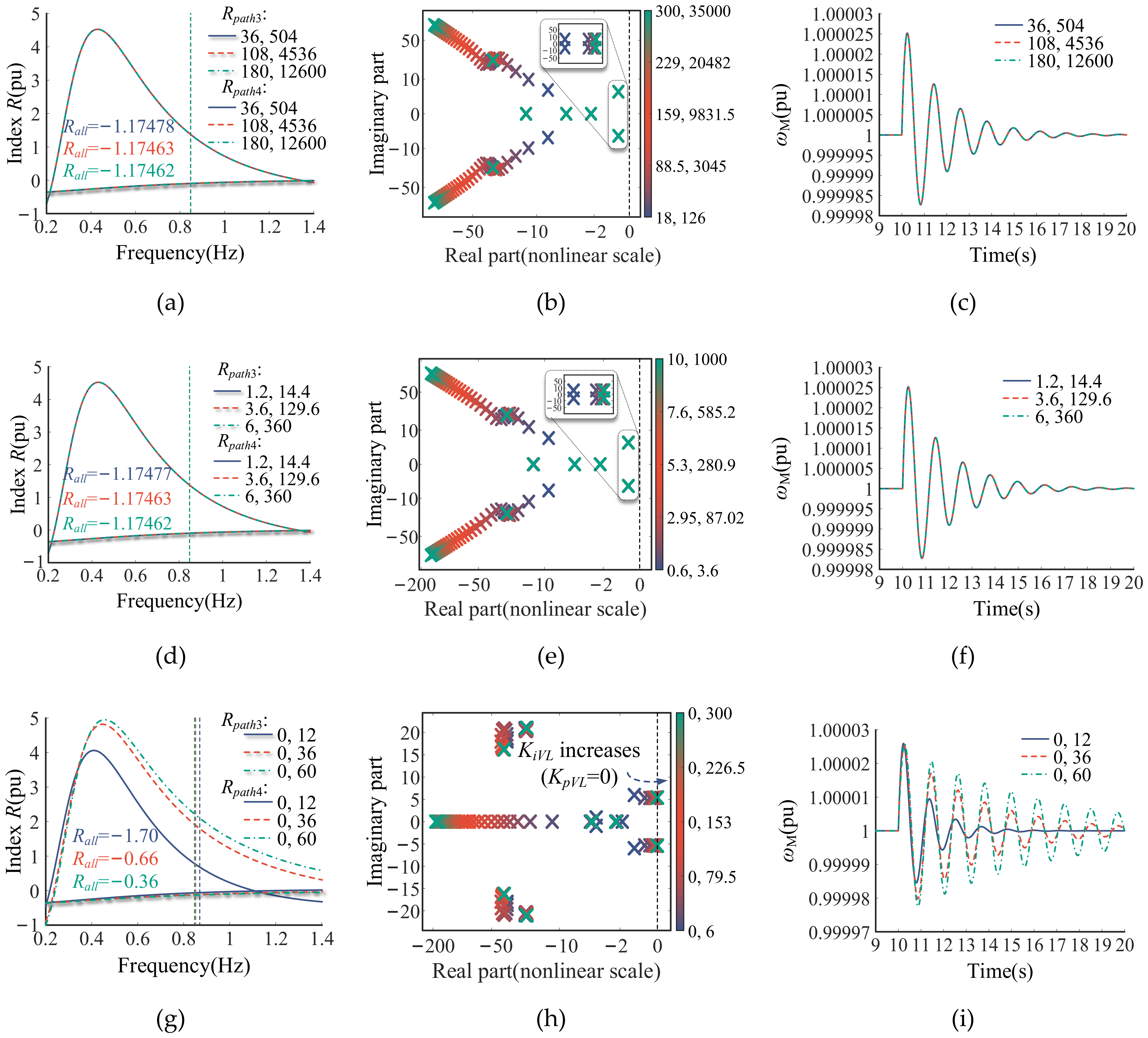
To further investigate the influence of the GFL converter on the synchronization stability of the GFM converter, the effects of different GFL control parameters on the R-based stability characteristics were evaluated. Since the analysis in this section focuses only on the GFL-related effects, the following analysis focuses on paths 3 and 4. The corresponding R contributions, root locus and EMT simulation results are presented in Figure 17.
Figure 17.
R index of each path, root locus and simulation waveforms under different control parameters. (a) Effects of PLL on R index of GFM; (b) root locus under different PLL control parameters; (c) ωM under different PLL control parameters; (d) effects of DVC on R index of GFM; (e) root locus under different DVC control parameters; (f) ωM under different DVC control parameters; (g) effects of TVC on R index of GFM; (h) root locus under different TVC control parameters; (i) ωM under different TVC control parameters.
As shown in Figure 17, Rpath3 was negative and Rpath4 was positive at the dominant oscillation frequency for all parameter settings. Moreover, the magnitude of Rpath4 was consistently greater than that of Rpath3, indicating that the GFL converter affected the GFM converter mainly through the indirect coupling path 4, while the direct path 3 provided a comparatively small stabilizing effect. As shown in Figure 17a, increasing Kppll and Kipll changed Rpath3 and Rpath4 only slightly, and Rall remained almost unchanged. The corresponding root locus results in Figure 17b show that the dominant eigenvalues almost overlap, while the time-domain responses in Figure 17c are nearly identical, further confirming that changing PLL parameters had little influence on the synchronization stability of the GFM converter. Similarly, Figure 17d shows that the R contributions under different DVC parameters almost overlap, as verified by Figure 17e,f. Figure 17g shows that increasing KpVL and KiVL increased Rpath4, whereas Rpath3 changed only slightly. Consequently, the variation in Rpath4 dominated the increase in Rall. Although Rall remained negative, the damping of the dominant oscillatory mode decreased as KpVL and KiVL increased. This trend is consistent with the corresponding root locus results in Figure 17h and simulation results in Figure 17i.
Overall, the GFL-related interaction paths yield a net positive R contribution to the GFM synchronization loop and therefore exert a destabilizing effect, mainly through the coupling path 4. Furthermore, changing the PLL and DVC parameters had little influence on the system stability, whereas increasing the GFL TVC parameters increased the positive contribution of path 4, thereby reducing the GFM stability margin.
4.3. Influence of GFM on the Synchronization Stability of GFL
The Rall of the system is given by Equation (23), where RC = Rpath1 + Rpathpll. The effects of the GFM control parameters on the R-based stability characteristics were investigated, with the analysis focusing on paths 3 and 4. The R contributions of the two paths, root locus and simulation results are shown in Figure 18.
Figure 18.
R index of each path, root locus and simulation waveforms under different control parameters. (a) Effect of TVC on R index of GFL; (b) root locus under different TVC control parameters; (c) ωL under different TVC control parameters.
As shown in Figure 18a, Rpath4 was negative at the dominant oscillation frequency for all parameter settings and decreased as KpVM and KiVM increased. Also, Rpath3 was initially positive but gradually decreased and became negative. The combined contribution Rpath3 + Rpath4 remained negative over the considered parameter range, indicating that the GFM-related interaction paths exerted a net stabilizing effect on the GFL synchronization loop. As KpVM and KiVM increased, both Rpath3 and Rpath4 decreased, making their combined contribution decrease and improving damping of the dominant oscillatory mode of the GFL converter. This conclusion is confirmed by the root locus results in Figure 18b and simulation results in Figure 18c.
Building on the preceding analysis, this section extends the path decomposition method to the GFL-GFM two-converter infinite bus system. With PSC and PLL selected as research objects, the feedback influence of the other converter was decomposed into several interaction paths. In particular, the dynamic contributions were separated into single-converter paths and the GFL-GFM coupling path, allowing the stability effect of each path to be quantified by R. The effects of key control parameters on R contribution were then characterized: changing the GFL PLL and DVC parameters had little influence on the stability of GFM. Faster TVC of GFL increased the positive Rpath4 associated with the coupling effect, thereby reducing the GFM stability margin. Faster TVC of GFM decreased both Rpath3 caused by the direct effect of GFM and Rpath4 co-determined by the coupling effect, enhancing the stability of GFL. The corresponding root locus and EMT simulation results then verify the R-based small-signal stability analysis, providing a methodological basis for parameter design in multi-converter systems.
5. Limitations
This study focused on the small-signal synchronization mechanisms of GFL and GFM converters using single- and two-converter infinite bus systems. The infinite bus assumption facilitates the separation of individual feedback paths, but practical networks may exhibit more complex interactions and operating conditions. In principle, the method can be extended to multi-converter systems by retaining the closed-loop dynamics of the other converters and constructing an equivalent network matrix; its scalability and accuracy in larger networks still require further investigation. In addition, the phase lags associated with the PLL and GFM inertia may interact with other control loops, such as DVC and TVC, making their effects on system damping more complex. The sensitivity of the R index to different control parameters can be used to identify their influence on the damping of the dominant oscillatory mode and provide guidance for parameter adjustment to suppress oscillations.
6. Conclusions
To clarify the individual synchronization stability mechanisms of GFL and GFM converters and the effects of their mutual interactions, this paper has established small-signal models of the two types of converters on the DC-link voltage timescale. A unified path decomposition method was adopted to comparatively analyze the similarities and differences between GFL and GFM in the single-converter infinite bus scenario, and their coupling characteristics in the two-converter infinite bus model were analyzed. The main conclusions are as follows:
- (1)
- In the single-converter infinite bus scenario, when the respective synchronization loop is selected as the research object, the overall feedback path from the output to the input of the synchronization loop of GFL and GFM can be decomposed into two paths: the purely algebraic AC network path Gpath1, and the dynamic control path Gpath2, which passes through both the AC network and the converter control loops. The stability effects of these paths are quantified by their corresponding R contributions. The R-based analysis, root locus and simulation results show that reducing Kpdc and Kidc improves GFL stability at high power levels (PL0 = 0.6–1.0 pu), whereas increasing these gains improves GFL stability at low power levels (PL0 = 0.1–0.5 pu, see Appendix D). Increasing KpVL and KiVL improves GFL stability in the investigated cases, while increasing KpVM and KiVM also improves GFM stability.
- (2)
- Under the unified path decomposition framework, the GFL and GFM converters have structurally analogous decomposition forms, but the characteristics of their corresponding paths differ. The R-based comparison further reveals their opposite responses to grid strength: as the grid becomes stronger, Rall decreases for the GFL converter but increases for the GFM converter. Consequently, the GFL converter exhibits better stability under strong-grid conditions, whereas the GFM converter exhibits better stability under weak-grid conditions.
- (3)
- In the GFL-GFM two-converter infinite bus system, when studying the influence of one device on the other, the overall feedback path from the output of the synchronization loop to its input can be decomposed into several interaction paths for both research objects: path 1, solely determined by the AC network algebraic relationship; paths 2 and 3, the single-converter paths determined by the dynamics of each converter; and path 4, the coupling path reflecting the combined effect of GFL and GFM. The R contribution of each path is quantified to evaluate the effect of one device on the other. Overall, the GFL-related paths yield a net positive R contribution to the GFM synchronization loop, whereas the GFM-related paths yield a net negative R-contribution to the GFL synchronization loop. Changing the GFL PLL and DVC parameters has little influence on GFM stability, while increasing KpVL and KiVL may destabilize the nearby GFM. Increasing KpVM and KiVM makes the net stabilizing effect on the GFL synchronization loop more negative, thereby improving GFL stability.
In summary, this paper explains the small-signal synchronization stability mechanisms of GFL and GFM converters from a unified theoretical perspective and establishes a small-signal model of the GFL-GFM two-converter infinite bus system. By combining the path decomposition method with the R-based analysis, the proposed method quantitatively distinguishes the stability contributions of single-converter and GFL–GFM coupling paths and clarifies the causes of oscillations on the DC-link voltage timescale. These findings are further validated by the root locus analysis and corresponding EMT simulation waveforms. The results provide a structured analysis tool for stability assessment and coordinated parameter optimization of multi-converter systems.
Author Contributions
Conceptualization, P.L. and Y.Z.; Methodology, P.L., Y.W. and Y.Z.; Software, Y.W.; Validation, Y.W. and W.W.; Formal analysis, Y.Z.; Resources, Y.W.; Data curation, W.W.; Writing—original draft, P.L. and Y.Z.; Writing—review and editing, Y.Z. and W.W.; Visualization, W.W.; Supervision, Y.W. and Y.Z.; Funding acquisition, P.L. All authors have read and agreed to the published version of the manuscript.
Funding
This research was funded by the Northwest Branch of the State Grid Corporation of China, Xi’an, Contract number: SGNW0000FGJS2500123.
Data Availability Statement
The original contributions presented in this study are included in the article. Further inquiries regarding the data can be directed to the corresponding author.
Acknowledgments
During the preparation of this study, the authors used Matlab R2021a for the purposes of analysis of GFL and GFM converters. The authors have reviewed and edited the output and take full responsibility for the content of this publication.
Conflicts of Interest
The authors declare that this study received funding from the Northwest Branch of the State Grid Corporation of China, Xi’an. The funder was not involved in the study design, collection, analysis, interpretation of data, the writing of this article or the decision to submit it for publication. The authors declare no conflicts of interest.
Appendix A. System Parameters and Supplementary Model Derivations
Appendix A.1. System and Control Parameters
All cases used a nominal frequency of fb = 50 Hz, an infinite bus voltage magnitude of Ug0 = 1.05 pu, a nominal DC-link voltage of Vdc0 = 1200 V and steady-state terminal voltage magnitudes of VL0 = VM0 = 1 pu for the GFL and GFM converters, respectively. In both single-converter systems, the total network impedance was Zall = (0.074 + j0.88) pu.
The common GFL controller settings were Cdc = 0.04 pu, (Kpdc, Kidc) = (2, 40), (Kppll, Kipll) = (60, 1400), and (KpVL, KiVL) = (0, 20). The common GFM controller settings were (KpVM, KiVM) = (1.5, 5) and (H, D) = (2.5, 20).
Table A1 and Table A2 list the remaining parameters for the GFL and GFM single-converter infinite bus systems studied in Section 3, respectively. Table A3 lists those for the two-converter infinite bus system studied in Section 4, with the active power settings distinguished by subsection.
Table A1.
Parameters of the single-converter infinite bus system containing GFL.
Table A2.
Parameters of the single-converter infinite bus system containing GFM.
Table A3.
Parameters of the two-converter infinite bus system.
Appendix A.2. AC Network Relationships and Path Expressions
Equation (9) can be written in polar form:
Thus, the partial derivatives of the magnitude and phase of Vt with respect to the magnitude and phase of Ic are as follows:
Appendix B. Validation of the Simplified Model
As discussed in Section 2, the dynamics of AC network inductors and capacitors and the current-loop dynamics are neglected in the simplified model. On the timescale considered in this paper, the current loop responded much faster than the synchronization and outer control loops, allowing the converter current to track its reference almost instantaneously. Meanwhile, the network impedances and their algebraic voltage–current relationships were retained.
Figure A1.
Comparison of time-domain responses obtained from the detailed and simplified models. (a) ωL in the single-converter GFL infinite bus system; (b) ωM in the GFL–GFM two-converter infinite bus system.
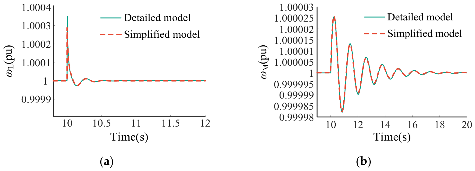
To validate this approximation, following the modeling approaches in References [9,24], the simplified model was compared with a detailed time-domain model that retained the current loop and AC network dynamics. Figure A1a compares the responses of ωL in the single-converter GFL infinite bus system, while Figure A1b compares those of ωM in the GFL–GFM two-converter infinite bus system. The waveforms obtained from the two models nearly overlap in both cases, indicating that the neglected fast dynamics had limited influence on the investigated synchronization responses. These results support the validity of the simplified model for the small-signal synchronization stability analysis conducted in this paper.
Appendix C. Derivation and Applicability of the R Index
The proposed R index focuses on the damping of the dominant oscillatory mode, enabling quantitative assessment of how different control loops or devices contribute to the corresponding oscillatory mode. Focusing on a dominant mode is a common assumption in power system small-signal stability studies, particularly in damping-based or equivalent SISO analyses [27,28,30,31,32], since different oscillatory modes are generally associated with different operating conditions or parameter combinations. If multiple poorly damped modes coexist, the proposed method can be applied separately to each dominant frequency, ωd1, ωd2, ωd3. In this paper, eigenvalue analysis was first used to identify the dominant oscillatory mode, after which the R index was applied to quantify the influence of different control loops or system components on its stability.
Figure A2.
Clarification of the R index.
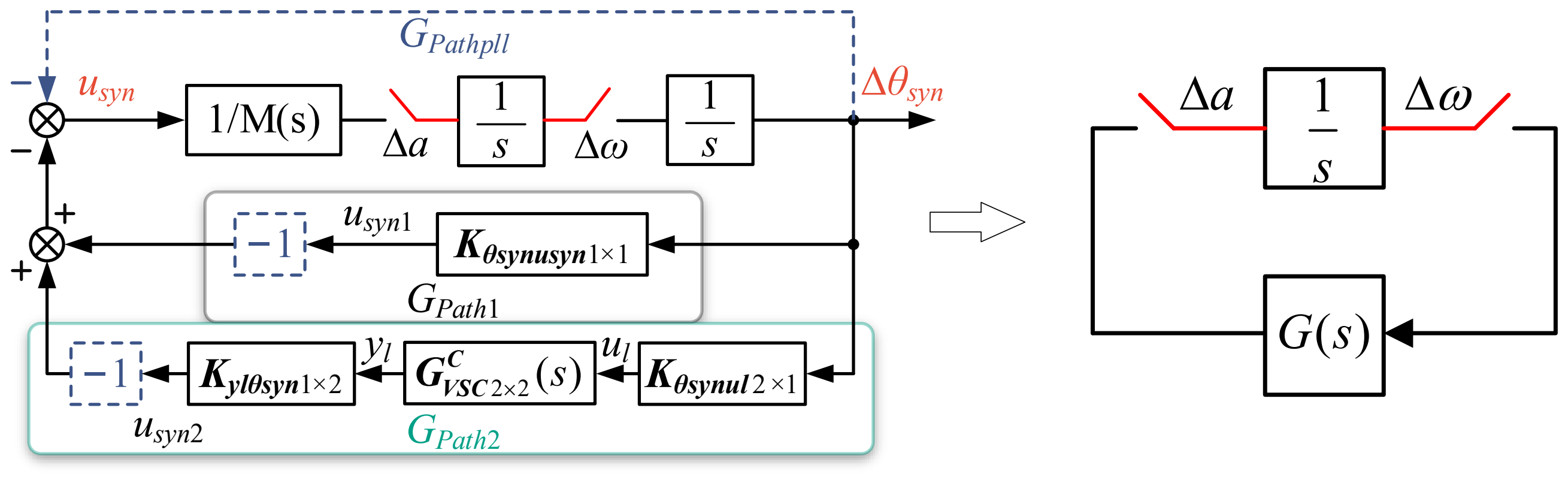
For a dominant, lightly damped oscillatory mode with an eigenvalue close to the imaginary axis, the R index can be used to characterize the damping of this mode. The following derivation illustrates this relationship using the equivalent system shown in Figure A2:
The closed-loop characteristic equation of the system shown in Figure A2 is
Define the real and imaginary parts of the frequency response of G(s):
where R(ω) is the proposed index.
For a lightly damped mode close to the imaginary axis, the estimated oscillation frequency ωd is given as
And the index for stability analysis is
Let λ denote the corresponding nearby eigenvalue. Then,
By performing a first-order Taylor expansion of the characteristic equation at (0, jωd), we obtain
where Fs’ denotes the derivative of F with respect to s.
Hence,
And
Since
where Gω’, Rω’, Iω’ denote the derivatives of G(jω), R(ω) and I(ω) to ω, respectively.
Therefore,
Hence,
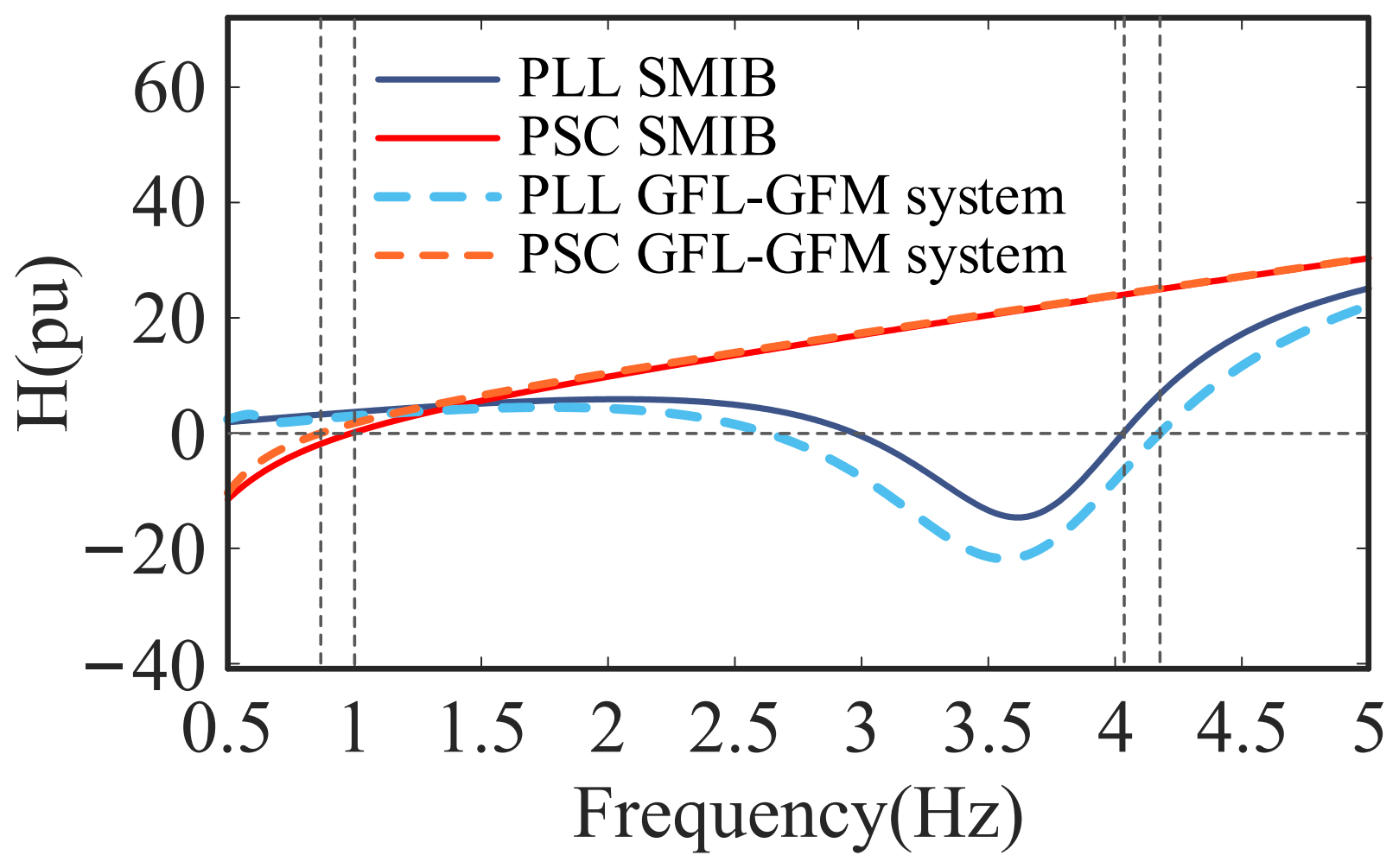
Therefore, when Hω’(ωd) > 0, R(ωd) and σ have the same sign. It should be noted that H(ω) is similar to the concept of “stiffness” in conventional power systems. In general, Hω’(ωd) is positive, meaning that the H(ω) curve crosses the horizontal axis from negative to positive at ωd. Owing to the diversity of power system devices and network configurations, a rigorous theoretical proof of this property has not yet been established. Nevertheless, this assumption underlies many equivalent SISO-based stability analysis methods and has been widely adopted in previous studies [28,30,31]. The present paper likewise does not attempt to provide a general proof of this property; instead, the corresponding H(ω) curves for the studied cases are presented in Figure A3 for verification.
Figure A3.
H(ω) in the studied cases.
Appendix D. Effects of Operating Power Levels on Stability Trends
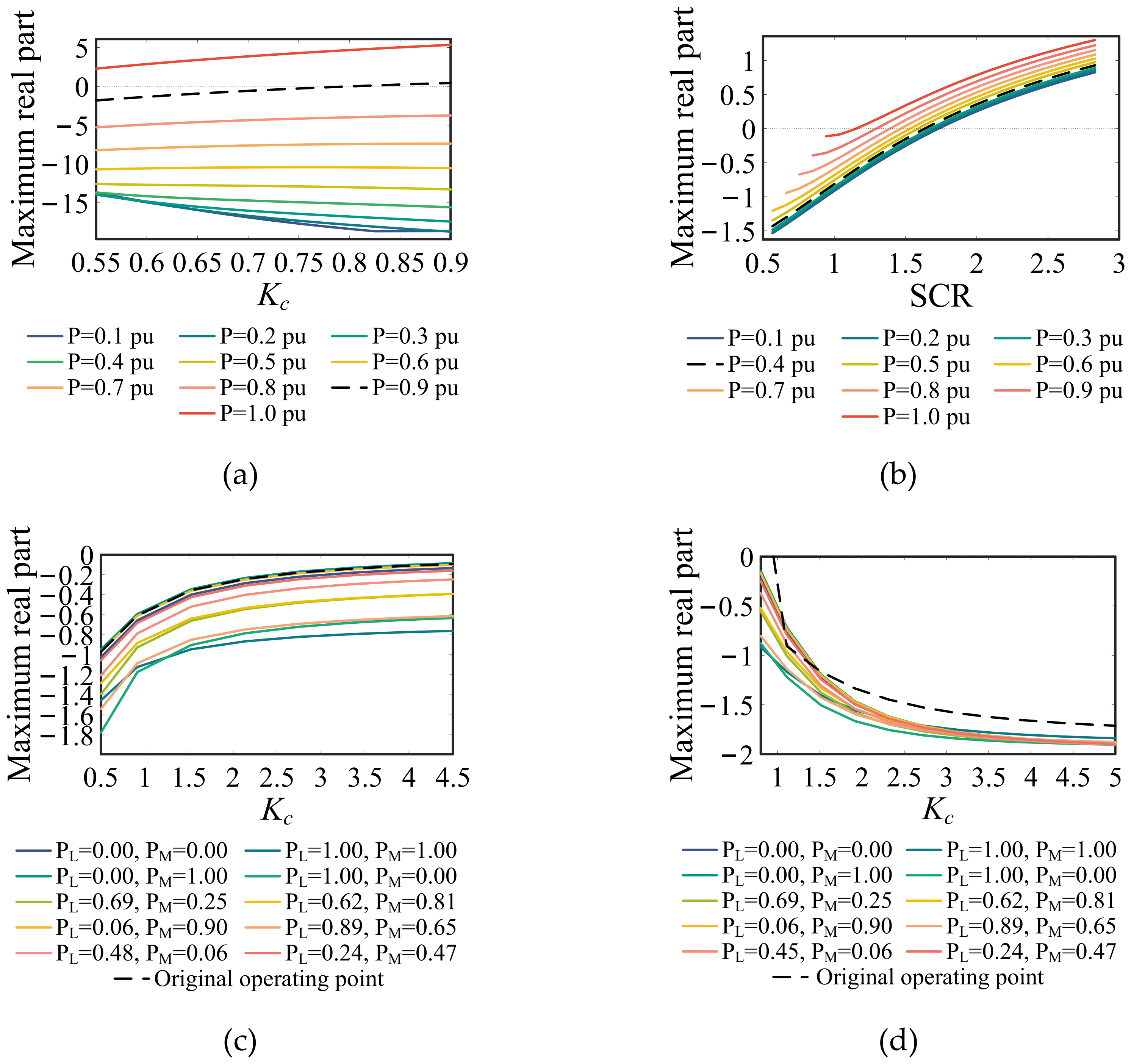
Further analysis reveals that the effects of the control parameters on system stability were generally consistent under different power levels, with an exception observed in the single-converter GFL system. To illustrate this, several representative cases are presented in Figure A4. For the control parameter variations, the proportional and integral gains of the second-order PLL and DVC loops were multiplied by Kc and , respectively, while both gains of the first-order TVC loop were multiplied by Kc. The horizontal axis represents the parameter Kc or SCR, while the vertical axis represents the real parts of the dominant eigenvalues. Different colors and line styles correspond to different active power levels.
Figure A4a shows the influence of DVC control parameters on the stability of the single-converter GFL system. At relatively high power levels PL0 = 0.6–1.0 pu, the real parts of the dominant eigenvalues increased as Kc increased, indicating deteriorating system stability, which is consistent with the results presented in the manuscript. However, at relatively low power levels PL0 = 0.1–0.5 pu, the opposite trend was observed.
For the other investigated parameter variations, the stability trends remained consistent under different power levels, as illustrated by the representative results in Figure A4b–d.
Figure A4.
Effects of some parameters on system stability under different active power levels. (a) Effects of DVC control parameters on GFL stability in the single-converter system; (b) effects of SCR on GFM stability in the single-converter system; (c) effects of GFL TVC control parameters on GFM stability with PSC as the research object in the two-converter system; (d) effects of GFM TVC control parameters on GFL stability, with PLL as the research object in the two-converter system.
References
- Yuan, X.; Hu, J.; Cheng, S. Multi-Time Scale Dynamics in Power Electronics-Dominated Power Systems. Front. Mech. Eng. 2017, 12, 303–311. [Google Scholar] [CrossRef] [Scilit]
- Venkatraman, A.; Markovic, U.; Shchetinin, D.; Vrettos, E.; Aristidou, P.; Hug, G. Improving Dynamic Performance of Low-Inertia Systems Through Eigensensitivity Optimization. IEEE Trans. Power Syst. 2021, 36, 4075–4088. [Google Scholar] [CrossRef] [Scilit]
- Gross, L.C., Jr. Sub-Synchronous Grid Conditions: New Event, New Problem, and New Solutions. In Proceedings of the 37th Annual Western Protective Relay Conference, Spokane, WA, USA, 19–21 October 2010. [Google Scholar]
- ENTSO-E. Grid Incident in Spain and Portugal on 28 April 2025—Final Report; ENTSO-E: Brussels, Belgium, 2025. [Google Scholar]
- Hatziargyriou, N.; Milanovic, J.; Rahmann, C.; Ajjarapu, V.; Canizares, C.; Erlich, I.; Hill, D.; Hiskens, I.; Kamwa, I.; Pal, B.; et al. Definition and Classification of Power System Stability—Revisited & Extended. IEEE Trans. Power Syst. 2021, 36, 3271–3281. [Google Scholar] [CrossRef] [Scilit]
- Harnefors, L.; Wang, X.; Yepes, A.G.; Blaabjerg, F. Passivity-Based Stability Assessment of Grid-Connected VSCs—An Overview. IEEE J. Emerg. Sel. Top. Power Electron. 2016, 4, 116–125. [Google Scholar] [CrossRef] [Scilit]
- Wu, G.; Sun, H.; Zhao, B.; Xu, S.; Zhang, X.; Egea-Alvarez, A.; Wang, S.; Li, G.; Li, Y.; Zhou, X. Low-Frequency Converter-Driven Oscillations in Weak Grids: Explanation and Damping Improvement. IEEE Trans. Power Syst. 2021, 36, 5944–5947. [Google Scholar] [CrossRef] [Scilit]
- Huang, L.; Xin, H.; Dong, W.; Dörfler, F. Impacts of Grid Structure on PLL-Synchronization Stability of Converter-Integrated Power Systems. IFAC-PapersOnLine 2022, 55, 264–269. [Google Scholar] [CrossRef] [Scilit]
- Huang, Y.; Yuan, X.; Hu, J.; Zhou, P. Modeling of VSC Connected to Weak Grid for Stability Analysis of DC-Link Voltage Control. IEEE J. Emerg. Sel. Top. Power Electron. 2015, 3, 1193–1204. [Google Scholar] [CrossRef] [Scilit]
- Rocabert, J.; Luna, A.; Blaabjerg, F.; Rodríguez, P. Control of Power Converters in AC Microgrids. IEEE Trans. Power Electron. 2012, 27, 4734–4749. [Google Scholar] [CrossRef] [Scilit]
- Zhong, Q.-C.; Weiss, G. Synchronverters: Inverters That Mimic Synchronous Generators. IEEE Trans. Ind. Electron. 2011, 58, 1259–1267. [Google Scholar] [CrossRef] [Scilit]
- Lu, S.; Wang, T.; Liang, Y.; Cheng, S.; Cai, Y.; Wang, H.; Yang, J.; Sui, Y.; Yang, L. Low-Frequency Oscillation Analysis of Grid-Connected VSG System Considering Multi-Parameter Coupling. Comput. Model. Eng. Sci. 2023, 135, 2373–2386. [Google Scholar] [CrossRef] [Scilit]
- Wu, H.; Ruan, X.; Yang, D.; Chen, X.; Zhao, W.; Lv, Z.; Zhong, Q.-C. Small-Signal Modeling and Parameters Design for Virtual Synchronous Generators. IEEE Trans. Ind. Electron. 2016, 63, 4292–4303. [Google Scholar] [CrossRef] [Scilit]
- Liu, R.; Ding, L.; Xue, C.; Li, Y. (Ryan) Small-signal Modelling and Analysis of Microgrids with Synchronous and Virtual Synchronous Generators. IET Energy Syst. Integr. 2024, 6, 45–61. [Google Scholar] [CrossRef] [Scilit]
- Hong, Z.; Xu, H.; Hou, Z.; Zhan, M. Origin of Anomalous Instability of Grid-forming Converters Tied to Stiff Grid. IET Renew. Power Gen. 2023, 17, 2563–2574. [Google Scholar] [CrossRef] [Scilit]
- Chen, Y.; Du, G.; Li, B. Controller Voltage Feedback-Based Power Synchronization Control for Grid-Forming Inverters Under Wide SCR Fluctuations. Int. J. Circuit Theory Appl. 2025, 53, 7038–7055. [Google Scholar] [CrossRef] [Scilit]
- Rosso, R.; Engelken, S.; Liserre, M. Robust Stability Investigation of the Interactions Among Grid-Forming and Grid-Following Converters. IEEE J. Emerg. Sel. Top. Power Electron. 2020, 8, 991–1003. [Google Scholar] [CrossRef] [Scilit]
- Xin, H.; Liu, C.; Chen, X.; Wang, Y.; Prieto-Araujo, E.; Huang, L. How Many Grid-Forming Converters Do We Need? A Perspective from Small Signal Stability and Power Grid Strength. IEEE Trans. Power Syst. 2025, 40, 623–635. [Google Scholar] [CrossRef] [Scilit]
- Duong, H.-N.; Tran, L.; Vo-Duy, T.; Trovão, J.P.F.; Nguyễn, B.-H. Small-Signal Stability Analysis of Mixed Power System Integrating Grid Forming and Following Inverters-Based Resources. Math. Comput. Simul. 2026, 241, 562–581. [Google Scholar] [CrossRef] [Scilit]
- Hu, G.; Xin, H.; Tang, Y.; Huang, L.; Yang, Y. Reduced-Order Multi-Subsystems of Power Systems With Grid-Following and Grid-Forming Converters for Small-Signal Stability Analysis. IEEE Trans. Power Syst. 2026, 41, 555–571. [Google Scholar] [CrossRef] [Scilit]
- Ji, X.; Liu, D.; Jiang, K.; Zhang, Z.; Yang, Y. Small-Signal Stability of Hybrid Inverters with Grid-Following and Grid-Forming Controls. Energies 2024, 17, 1644. [Google Scholar] [CrossRef] [Scilit]
- Zuromski, C.; Becker, C. Small-Signal Stability and Interaction Analysis of Grid-Forming and Grid-Following Converters in Converter Dominated Power Systems. Munich, Germany, 17–18 September 2024. [Google Scholar]
- Gebremedhin, T.; Chen, Y.; Xu, L.; Chen, D. Impedance-Based Characterisation of Grid-Forming and Grid-Following Converter Interactions in Multi-VSC Systems. IET Renew. Power Gener. 2026, 20, e70319. [Google Scholar] [CrossRef] [Scilit]
- Zhou, Y. Study of Synchronization Mechanism Between Voltage/Current Rotating Vectors and Its Application in the Analysis of Interaction Between Devices. Ph.D. Thesis, Huazhong University of Science and Technology, Wuhan, China, 2024. [Google Scholar]
- Zhou, Y.; Miao, L.; Li, S.; Hu, J.; Zhu, D.; He, W. Mechanism Analysis of Interaction Between Synchronous Condenser and VSC. CSEE J. Power Energy Syst. 2024, Early Access, 1–12. [Google Scholar]
- Zhang, M.; Yuan, X.; Hu, J. Mechanism Analysis of Subsynchronous Torsional Interaction With PMSG-Based WTs and LCC-HVDC. IEEE J. Emerg. Sel. Top. Power Electron. 2021, 9, 1708–1724. [Google Scholar] [CrossRef] [Scilit]
- Harnefors, L. Analysis of Subsynchronous Torsional Interaction with Power Electronic Converters. IEEE Trans. Power Syst. 2007, 22, 305–313. [Google Scholar] [CrossRef] [Scilit]
- Yuan, H.; Yuan, X.; Hu, J. Modeling of Grid-Connected VSCs for Power System Small-Signal Stability Analysis in DC-Link Voltage Control Timescale. IEEE Trans. Power Syst. 2017, 32, 3981–3991. [Google Scholar] [CrossRef] [Scilit]
- Liu, Y.; Hu, J.; He, W.; Zhou, Y.; Zhan, M. Local Load Effect on the DC Voltage Control Timescale Oscillation of Voltage Source Converters. IEEE Trans. Power Syst. 2026, 41, 381–395. [Google Scholar] [CrossRef] [Scilit]
- Zheng, W.; Hu, J.; Chai, L.; Liu, B.; Sang, Z. Interaction Quantification of MTDC Systems Connected with Weak AC Grids. CSEE J. Power Energy Syst. 2024, 10, 2088–2099. [Google Scholar] [CrossRef] [Scilit]
- Wang, D.; Hou, Y.; Hu, J. Net Damping Criterion for Stability Analysis of Grid-Tied VSCs in DC Voltage Control Timescale. CSEE J. Power Energy Syst. 2020, 6, 601–609. [Google Scholar] [CrossRef] [Scilit]
- Tan, S.; Geng, H.; Yang, G. Phillips-Heffron Model for Current-Controlled Power Electronic Generation Unit. J. Mod. Power Syst. Clean Energy 2018, 6, 582–594. [Google Scholar] [CrossRef] [Scilit]


Disclaimer/Publisher’s Note: The statements, opinions and data contained in all publications are solely those of the individual author(s) and contributor(s) and not of MDPI and/or the editor(s). MDPI and/or the editor(s) disclaim responsibility for any injury to people or property resulting from any ideas, methods, instructions or products referred to in the content. |
© 2026 by the authors. Licensee MDPI, Basel, Switzerland. This article is an open access article distributed under the terms and conditions of the Creative Commons Attribution (CC BY) license.