


Abstract
Sparse greenhouse surrogates are often selected by prediction accuracy, although their purpose is feedback control. We compare three sparse identification of nonlinear dynamics (SINDy) libraries and 15 controllers in a GreenLight tomato greenhouse using reanalysis weather. The identification ladder comprises 54 distinct recipes at 20 seeds. Physical features reduce mean one-step temperature root mean square error from 1.86 to 1.68 °C but increase median 24 h error from 2.67 to 23.79 °C; CO2 and humidity show the same reversal. Labelled numerical-completion and planner-cap variants yield a mixed cohort of 1048 full trajectories across four 60-day test seasons. The raw ensemble has the highest reference-setting mean margin (+4.32 EUR m−2), with 4140 climate-corridor variable-steps; the low-threshold intermediate controller achieves +3.07 with 3699, while proximal policy optimisation achieves +0.45 with 1330. Training-selected horizons and price-dependent selection retain the raw ensemble’s largest mean among four principal sparse configurations at all nine prices, without adjusted separation from the nearest comparator at nominal prices. Weather interventions, crop-state continuations and paired coefficient edits assess mechanisms and robustness. The inner model predictive controller predicts climate and resource use, not crop revenue; seasonal margin is evaluated separately. Results support complementary multi-step, interpretability and closed-loop checks within the tested sparse-identification setting.
1. Introduction
Protected tomato production depends on maintaining a productive microclimate while containing the variable costs of heating, supplementary lighting and CO2 enrichment. These inputs affect crop growth and resource use simultaneously, so a control strategy should be judged agronomically and economically rather than by setpoint tracking alone [1,2,3]. Here, economic model predictive control (MPC) weights climate deviations and resource use over a finite horizon [4,5,6]. Simulated crop revenue enters the seasonal evaluation, not the MPC stage cost.
Simulation-based greenhouse studies are established in this application area. Xu et al. used a greenhouse–crop model to compare open- and closed-loop optimal control and to estimate lettuce yield and profit in an explicitly computational study [7]. Wen et al. combined measured blueberry photosynthesis with an SVR model and simulated multi-objective light–CO2 regulation [8], while Ećim-Đurić et al. coupled a TRNSYS greenhouse model to an artificial neural network and anchored the thermal model to measured temperatures [9]. These examples show both the value and the evidential limit of simulation: virtual experiments can isolate controller and model-design effects, but field performance requires empirical anchoring.
MPC requires a process model, and calibrating a detailed mechanistic greenhouse model for every site is laborious. A surrogate identified from simulated or measured trajectories can reduce that burden. Sparse identification of nonlinear dynamics (SINDy) is attractive because it expresses the dynamics as a sparse combination of library functions [10,11,12,13]. Unlike a neural surrogate, the resulting equations can be inspected for physical and dimensional consistency and embedded analytically in an MPC solver.
Three benchmarking risks complicate an objective comparison of such surrogates. First, learned controllers may be compared with an unsearched heuristic even though tuned agronomic rules are a strong reference [14,15,16]. Second, a setpoint-tracking index may be reported instead of economic margin [6,14], although the two need not be monotonically related. Third, surrogate hyperparameters are commonly selected by one-step prediction accuracy [12,17], implicitly assuming that the best short-horizon predictor also gives the best controller. The benchmark addresses these risks through a tuned heuristic, an economic score and a multi-step model check.
Identification for control and multi-step validation are established ideas [17,18,19,20,21,22,23,24,25,26]. Prediction accuracy alone need not measure the value of a model inside a feedback policy. Here, sparse-library design is the experimental factor: its added physical transforms reuse measured variables and can change conditioning and term selection [27,28,29,30,31].
The scientific contribution has three connected parts. First, a matched sparse-library experiment establishes the reversal between one-step accuracy and multi-step stability for temperature, CO2 and humidity. Second, controlled library contrasts, threshold sweeps, term deletion and paired coefficient edits examine actuator-pathway survival and test a proposed explanation that the data ultimately do not support. Third, seasonal control trials, training-only tuning and weather/crop-state checks establish where prediction-based selection agrees with realised margin and where further closed-loop evaluation remains necessary. The evidence concerns this combination of library design, mechanism tests and economic–climate outcomes; rollout error itself is an established diagnostic [17,18,19,20,21,22,23,24,25,26].
The experimental programme includes an identification ladder, a 15-controller benchmark, threshold sweeps, term-deletion and coefficient-edit experiments, observer and guard tests, fault supervision and price/parameter sensitivities. A baseline scalar series supplies the mechanism and supporting experiments. A primary-environment series supplies matched comparisons, training-only horizon and price-dependent policy selection, weather and crop-state checks, actuator diagnostics and numerical portability. Complete designs and outcomes are given in the Supplementary Information and data; cohort and protocol identifiers distinguish these series.
2. Materials and Methods
2.1. Simulation Study Design Weather and Experimental Units
The simulated house is at Rostov-on-Don (47.24° N, 39.71° E). Weather forcing came from the ERA5/ERA5-Land reanalysis [32] via Open-Meteo (OpenMeteo GmbH, Bürglen, Switzerland) [33]; sky temperature was derived from the retrieved dew point and cloud cover, and the deep-soil boundary condition was refitted as a single annual harmonic to ERA5-Land soil temperature at this site, replacing the simulator’s Dutch default. Outdoor CO2 was held at 400 ppm, a limitation of the model. A season contains 5760 control intervals of 900 s. The loader convention applies a one-based start-day index to a zero-origin annual series, so the scenario requested as 1 March consumes forcing from 2 March. All comparisons preserve this convention. Exact consumed-prefix weather summaries, rather than an assumed calendar label, are supplied in Table S16.
Training trajectories were collected by the rule-based controller over both training seasons (two 60-day trajectories of 5760 control steps per replicate) with a pseudo-random binary excitation of amplitude 0.3 on each of the six actions, redrawn every 16 steps (4 h), plus a zero-mean Gaussian perturbation of standard deviation 0.1 redrawn every 5 steps, the sum clipped to the actuator bounds. Evaluation rollouts carry no excitation. All greenhouse, crop and actuator parameters use the default GreenLight tomato configuration, and the virtual crop starts every season from its default initial state (software configuration in Section S22); only the weather files and the deep-soil boundary described above were changed.
The main evaluation covers 2020–2023. Additional 2014–2017 seasons test the principal sparse configurations with the priced objective and 20 seeds; a separate four-controller default-objective study with eight seeds remains available. Calendar year alone does not establish a distribution shift. We therefore call all evaluated years test years and quantify weather differences and trajectory extrapolation instead of labelling 2020 in-distribution and the other years out-of-distribution.
An identification seed regenerates both the excitation data and the fitted surrogate; weather years repeat the same fitted model. Proximal policy optimisation (PPO) and soft actor–critic (SAC) seeds regenerate policy training. Every stochastic controller has 20 seeds in the matched benchmark. The two deterministic heuristics each have one trajectory per year and no artificial seed replication. Reused trajectories retain every requested logical condition, including different prices, while their shared physical origin is recorded.
Weather comparisons use the exact control-grid prefix consumed by the loader. Hourly calendar-window summaries form a separate reconstruction, so their dates and radiation weights are not interchanged with simulation-step summaries.
2.2. Economic Criterion and Climate Exposure
Controllers are scored by the profit term of the simulator’s own reward function; no tracking-error proxy is used. At step k, that term is a marginal income πk, and the seasonal economic performance indicator (EPI), written J throughout, is
where gk is income from modelled fruit dry-matter growth, converted to fresh mass with a dry-to-fresh ratio of 0.065 and valued at 1.60 EUR/kg, and ck is the variable costs of heating (0.09 EUR/(kW·h)), supplementary lighting (0.30 EUR/(kW·h)) and CO2 enrichment (0.30 EUR/kg). Labour, planting material, water, fertiliser, depreciation and fixed costs are excluded. Revenue is modelled as net fruit growth, not measured marketable harvest. The fruit already present at the accounting boundary has contributed through its growth; valuing the same stock again would double-count revenue.
The MPC surrogate has temperature, CO2 and relative-humidity states, but no crop-growth or biomass state. Its resource-aware stage cost is described in Section 2.6; it does not optimise predicted crop revenue. Seasonal J is calculated afterwards in the separate greenhouse–crop simulator. PPO and SAC use their specified training reward, which also penalises corridor violations, whereas all controllers are evaluated using the same unpenalised seasonal margin. Differences between these objectives remain part of the stated implementations.
The evaluation corridors are 15–34 °C, 300–1600 ppm CO2 and 50–85% relative humidity. For each variable, we record the number of intervals outside its corridor, the duration (count × 0.25 h), and the magnitude of the excursion. The main climate outcome is the sum of the three violation counts, called corridor variable-steps; one interval can contribute to more than one variable. Separate duration and exceedance measurements are reported in Table S4. These outcomes are observed simulation metrics, not a recursive-feasibility or agronomic-safety guarantee.
Final crop-state effects are examined by transferring all 28 process states from each complete 60-day parent into another 60-day season under either the stock or the tuned common heuristic. Weather remains continuous across the handover, and no crop state is reset. We report the parent, continuation and combined margins. This assesses later productive effects of leaves, stems and reserves without adding terminal fruit revenue a second time. Incomplete parent records and their separately labelled completed parent variants remain distinguishable.
This corridor is also not the one the predictive controllers minimise against: their stage cost (Section 2.6) penalises humidity only above 85 % and CO2 only below a floor, so the lower humidity and upper CO2 bounds are unweighted in the optimisation yet counted on the violation axis. Margin–exposure comparisons therefore report common realised outcomes rather than adherence to identical optimisation penalties. Mean exceedance is computed over violating steps within each trajectory; zero-violation trajectories contribute zero. It is neither the maximum excursion nor an extrapolation of a short season.
A baseline-series accounting diagnostic expressed margin gaps as break-even extra future fruit dry-matter growth: 20, 50, 64 and 157 g m−2 for the baseline-series plain-raw, low-threshold, full-physics-ensemble and PPO contrasts. These are calculated thresholds, not observations of missing harvest. They must not be added to the already counted terminal fruit stock. The full-state continuation experiment instead measures later productive effects under two declared common policies.
2.3. Controllers Compared and Computational Allocations
The 15-controller benchmark includes nine sparse MPC definitions, neural MPC, PPO, SAC, a full-model planner and stock/tuned heuristics [34,35,36]. Four principal sparse configurations are used in the matched extensions: raw ensemble, frozen intermediate ensemble, low-threshold intermediate fitted by sequentially thresholded least squares (STLSQ) and full-physics ensemble. Only the three ensemble configurations form a complete one-factor library comparison at the same fitting recipe. The low-threshold controller is a strong physics-feature competitor with a different threshold and estimator, not an isolated library intervention. Complete definitions, including the two additional 17-feature term-deletion probes, appear in Table S1. The controller families and their declared training and planning allocations are summarised in Table 1.
Table 1.
Controller families and declared training or planning allocations. These are different forms of effort, not equal computational budgets. The four principal sparse configurations receive the stated horizon/weight searches; PPO and SAC retain their stock hyperparameters.
The aggregation loop applied to two SINDy controllers rolls the learner’s own MPC in a closed loop in the training seasons, appends the visited states to the identification set and re-estimates the model (3 iterations of 5-day episodes). They receive no expert demonstrations and do not implement DAgger imitation learning [37]. Their aggregation uses the default objective while the main evaluation uses priced weights, an asymmetry retained in the interpretation.
Five of the SINDy-MPC labels form a deliberate one-factor design over the feature library, and the mechanism analysis of Section 3.5 rests on it. The ensemble arm is a complete three-point series; the STLSQ arm has only the two endpoints, because the two STLSQ controllers using the intermediate library were frozen at thresholds 10−3 and 10−6 rather than 0.05. The two additional 17-feature probes lie outside the 15-controller benchmark.
The baseline timing log records median test-season rollout times of 4.7 s for the stock rule, 5.6/5.9 s for PPO/SAC inference, 70–79 s for the five sparse MPCs in that series, 1867 s for neural MPC and 6996 s for the full-model planner. These are series-specific measurements, excluding identification and policy training. They establish the practical cost of seasonal trials in that implementation, not hardware-normalised or equal-budget limits of the controller families.
2.4. Feature Libraries and Sparse Identification
Sparse regression [10,11,12] recovers an explicit discrete one-step map
with state xk = (Tin,c,φ)⊤ (air temperature, CO2, relative humidity), six controls uk (boiler, CO2 injection, thermal screen, ventilation, lamps, blackout screen) normalised to [0, 1], and disturbances dk (outdoor temperature, global radiation, outdoor CO2, two diurnal harmonics). Three feature libraries were compared, differing only in :
- Raw library—11 features: the five disturbance channels and the six controls, with no state transform;
- Intermediate library—those 11 plus three physically motivated transforms of state, radiation and screen position (14 features): saturation vapour pressure es(Tin) = 0.6108exp(17.27 Tin/(Tin + 237.3)) by the Magnus–Tetens relation, vapour-pressure deficit D = (1 − φ/100) es, and screen-attenuated radiation Seff = I (1 − uthscr);
- Full-physics library—those 14 plus four bilinear state × control cross terms (TinSeff, φuvent, (c − cout)uvent, Tinuboil), 18 features.
The three climate states and an intercept accompany each feature set. States and features are standardised before regression, and native-unit coefficients and scalers are retained. The Magnus–Tetens transform uses temperature in °C and produces saturation vapour pressure and vapour-pressure deficit in kPa. The constant 400 ppm outdoor-CO2 feature becomes zero after centring; the standardisation uses scale one for that zero-variance column. It contributes no information about outdoor-CO2 variation. A separate bias term supplies the intercept. The reported finite condition ratio uses the nonzero singular spectrum before adding that bias; the full rank-deficient matrix has an infinite condition number.
The three physical functions are nonlinear transforms of variables already in the raw library and add near-collinear columns without any new measurement. In every library, the three states and a constant enter the degree-1 candidate set alongside the listed features, so each state equation selects from 15, 18 and 22 columns for the raw, intermediate and full-physics libraries (21 for the deletion library), that is 45, 54, 66 and 63 candidate coefficients in .
The ensemble optimiser uses 20 bagged bootstrap replicates [13]. These are internal models within one fitted ensemble, distinct from the 20 identification seeds that regenerate excitation data and fitted surrogates. Repeated ensemble draws on the same identification dataset form a separate design axis: 10 draws per seed in the canonical wave and 6 in the later wave that added the raw-library controller.
2.5. Identification Ladder and Retrospective Selection Audit
The ladder combines three libraries, two polynomial degrees, four recorded optimiser labels and three denoisers at 20 seeds: 1440 labelled fits. After duplicate removal, there are 54 distinct recipes rather than 72 independent configurations (Section 2.9). The main comparison uses analytic degree-one models; degree-two candidates remain in the ladder but fail the implemented MPC-embedding gate.
One-step errors and free-running 4-, 20- and 96-step errors are evaluated for temperature, CO2 and humidity in native units. Up to 20 equally spaced starts are advanced using recorded inputs. A free-running path fails after an exception, non-finite prediction or absolute state value above 106 in any native unit. Root mean square error (RMSE) uses valid prefixes and is accompanied by failed-path counts, so an early numerical failure cannot be interpreted as a successful low-error rollout. Same-year and cross-year prediction checks are retained separately.
The frozen recipe is the undenoised, degree-one intermediate library with ensemble fitting. The selection audit is explicitly retrospective. It removes the duplicated estimator label, retains analytically embeddable recipes with mean divergence fraction at most 0.05, and ranks them by 24 h temperature RMSE, active-term count and recipe name. The transparency gate requires sign-pass fraction ≥ 0.5, bootstrap active-term stability ≥ 0.6, complete unit metadata and native prediction equivalence. Table S17 defines these checks and the pooled divergence statistic, distinct from the 96-step failures in Table 2. Required seed-pass fractions of 0.5, 0.9 and 1.0 are evaluated separately. Selection chooses a recipe rather than a favourable seed; the audit follows observation of the test-year outcomes.
Table 2.
Prediction errors for degree-one undenoised STLSQ/ensemble fits, 40 labelled fits per library. One-step entries are mean RMSE; 24 h entries are median valid-prefix RMSE. The path-failure criterion is joint across the three states, so its fraction repeats within each library. Humidity pp denotes percentage points.
2.6. MPC Formulation and Resource-Aware Stage Cost
The explicit form of Equation (2) allows it to be embedded analytically in a finite-horizon optimal control problem [4]:
with N = 20 steps (5 h), Δuk = uk − uk−1 and R = diag(10, 5, 100, 50, 1, 1) in the actuator order of Section 2.4 (boiler, CO2, thermal screen, ventilation, lamps, blackout screen). The corridor term is , where bT, bc and bφ are excursions from a diurnally varying productive band: temperature in [15 + 3w, 19 + 5w] °C, CO2 above 400 + 300w ppm and relative humidity below 85 %, with w ∈ [0, 1] being a smooth day weight. Deviations from the productive bands are penalised softly, but the hard bounds can still make a numerical solve infeasible; the temperature bounds [12,38] °C, the ventilation bound 0.4 and the unit box on the other controls are hard constraints, and the move-suppression term penalises control increments. The problem is solved by an interior-point method (IPOPT 3.14.11, bundled with CasADi 3.7.2 [39] through do-mpc 5.1.1 [40]), whose initial guess is set once from the measured initial state and carried forward by the solver itself; no controller-specific warm start is supplied. The unmodified solver-based protocol permits 100 caught solver or planner exceptions per run. Each exception triggers a fixed fallback action (boiler 0.3, thermal screen closed, all else zero); the 101st exception stops the run before another action and the 100-exception capped result is retained separately (Section 2.8).
Two resource-weight variants were evaluated in . The default implementation uses , a ratio of 1:0.5:0.1. The primary priced formulation therefore uses , scaled so the total at u = (1, 1, 1) is 31.99 against 32.0 under the default formulation. These are stage-cost weights, not a prediction of crop revenue. The climate and move coefficients are fixed engineering choices rather than monetary prices.
The nominal resource weights and their price-aligned variant leave climate and move penalties unchanged. Price alignment matches relative heating, lighting and CO2 costs but does not make the proxy a crop-profit objective, nor does an equal sum of resource weights preserve the resource–climate trade-off along different trajectories. We therefore vary the common resource and climate multipliers independently by 0.5 and 2, with move penalties fixed. Both economic and climate outcomes are retained.
The full-model planner uses 48 candidate control sequences in two cross-entropy rounds per step. It is a computationally constrained benchmark, not an upper bound on crop profit. Neural MPC permits 25 L-BFGS-B iterations and applies the returned action even when the optimiser reports an unsuccessful solve. Those flags, caught exceptions, actual fallback actions and available residuals are recorded separately. No controller family is claimed to have received an equal computing or hyperparameter-search budget.
The climate weights are engineering penalties: a 1 °C temperature-band miss, 100 ppm CO2 shortfall and one percentage point above the humidity ceiling contribute 30, 3 and 8 objective units per step. They are not crop-damage prices. Independent climate/resource multipliers test the balance of these penalties; matching actuator-cost ratios alone cannot make the climate-only model predict crop profit.
2.7. Rule-Based Reference and Training-Only Tuning
To avoid an unsearched baseline, the heuristic was given a 16-trial setpoint-search budget (Table S22). Sixteen configurations were drawn i.i.d. uniformly from a fixed pseudo-random generator (seed 20260810) and scored alongside the stock configuration, which enters the search as trial 0, giving 17 evaluated configurations. Selection used the mean of J over the training seasons 2018–2019 only; the test seasons play no part in it. This gives 17 profiles, 34 full training seasons and 195,840 control steps. Each profile is deterministic. A finite search improves the baseline comparison without claiming to find globally optimal agronomic settings.
For each principal sparse configuration, horizons 8, 12 and 20 are compared over 2018–2019 using 20 seeds. The selected horizon maximises mean training margin, with corridor exposure and shorter horizon as tie-breaks, and is then frozen for the four test years. Price-dependent selection extends this to 21 horizon–resource settings: the three horizons and resource multipliers 0.125, 0.25, 0.5, 1, 2, 4 and 8. At each of nine fruit/resource price pairs (multipliers 0.5, 1 and 2), training first favours completed seasons, then price-specific crop-growth revenue less resource cost, fewer violations, shorter horizon and smaller multiplier. The heuristic is independently reselected from its 17 candidate profiles. Test outcomes do not enter either choice. This finite outer search can change a policy with price; the inner MPC still has no crop-revenue forecast.
2.8. Experimental Contrasts and Statistical Treatment
The coefficient intervention is paired, not randomly assigned: for each fitted seed, the same baseline, boiler knock-in and boiler knock-out are evaluated. Knock-in copies the direct boiler coefficient from the same-seed low-threshold donor while leaving other coefficients unchanged; knock-out sets it to zero. The extension spans three specified recipes, four test years, two objectives and 20 seeds, adding 960 edited seasons. The intervention estimates the effect of this declared edit. Associations between unedited library-level term survival and margin remain observational. The baseline threshold sweep, four-test 2020 family and failed bilinear-detour test are preserved in Section S21.
All six actuator pathways are inspected with native-unit finite-difference Jacobians of the stored surrogate at up to 256 points per trajectory. Perturbations are clipped to command bounds, including the ventilation limit. Temperature, CO2 and humidity responses, response quantiles and negative fractions are recorded. Heating and direct CO2-injection signs receive their stated local checks; ventilation is conditional on inside/outside conditions and is not assigned one unconditional sign. Joint support uses the three states and six actions, standardised on each same-seed pseudo-random binary sequence (PRBS) reference, with range excursions and nearest-neighbour exceedances at training quantiles 0.95 and 0.99.
Coefficient sensitivity perturbs the dense-intermediate fitting recipe at 20 seeds and evaluates the 2020 season. Independent multiplicative Gaussian edits c(1 + εz) use ε = 0.02, 0.05, 0.10, 0.15 and 0.20, four draws per seed and zeros unchanged. The same 400 perturbed models are evaluated under default and priced objectives, giving 800 seasons. A pre-rollout local screen checks finite predictions within broad native-unit bounds and the direct heating/CO2 signs at 256 training coordinates. All perturbed models and the screen-passing subset are reported; the screen is not a global physical-consistency certificate.
A complete temperature × radiation × humidity factorial exchanges the 2020 and 2021 forcing components, at reference and training-selected horizons. Every factorial cell retains the recipient’s exact 28-state initial vector. All seven factorial contrasts and order-averaged component contributions are evaluated; the contributions sum to the joint forcing effect and include interactions. The default-reset weather experiment remains a separate initialisation sensitivity. Additional plant discrepancies modify only the simulator’s ventilation-command map (±0.25 curve parameter) or maximum fruit-growth sink (±20%), leaving each nominal controller unchanged.
For incomplete unmodified runs we show accumulated outcomes, completed seasons only and diagnostic outcomes per recorded day. A rate is not presented as an extrapolated full season. Comparisons use matched seed–year coordinates and distinguish cohort changes from controller changes. Exact and tolerance-based Pareto membership is supplemented by seed-bootstrap frequencies; the comparison using all 15 complete controllers and the retained 13-controller pool are separately identified. Tolerances of 0.025–0.10 EUR m−2 and 25–150 variable-steps are illustrative reporting choices. A numerical near-tie check is also included.
Effects are averaged across matched weather years within seed before inference. Descriptive 95% intervals use 30,000 seed-bootstrap draws [38,41]. SINDy comparisons retain identification-seed matching; PPO/SAC training seeds are independently resampled, and deterministic references remain fixed. Signed-rank tests [42] use Holm adjustment [43] within stated scientific families. The primary 2020 boiler-edit family has four tests; its extension has 12 margin tests. Principal-library, horizon, weight, price, weather and plant families are declared separately, with separate margin and corridor families. Descriptive intervals are not simultaneous confidence intervals. Year contrasts, leave-one-year sensitivity and a descriptive eight-year resampling analysis address weather sensitivity without treating one site’s years as a population of future climates. The feature-deletion contrasts use the same within-seed aggregation and a separate four-test family (Table S44).
Paired coefficient edits retain the same fitted model and seed except for the declared stored coefficient; refitting a deleted library changes other coefficients as well. These designs cannot be pooled as one intervention. Weather years repeat a fitted seed, and repeated ensemble draws likewise do not become independent identification cases. Deterministic weather-matched references supply constants rather than a second stochastic sample. A two-sided exact signed-rank test based on only four weather observations has minimum attainable p = 0.125; such a test cannot establish 5% significance.
Effect sizes accompany every p-value, with medians preferred to means wherever the distribution is skewed, and bootstrap confidence intervals [38,41] for aggregate quantities. Bootstrap intervals condition on their named weather years; they are neither simultaneous intervals for every comparison nor a distribution of future climates. Duration and fallback percentages use recorded steps, including early stops, and do not imply a completed remainder.
2.9. Reproducibility and Numerical Completion
The completion audit distinguishes unmodified attempts, exact repeats and completion variants within the primary-environment campaigns. Here, 288 logical rollout conditions mapped to 280 distinct physical settings that stopped early; another 122 continuations had incomplete parents. Exact repeats used the saved models, forcing and settings. At 260 physical settings, the native integrator again failed to converge: the condensation formula had a finite right-hand side but an overflowing automatically differentiated Jacobian. An algebraically equivalent stable expression passed each rejected checkpoint without changing physical parameters, tolerances, solver step allowance, state limits or stopping guards. Each affected season was restarted. These numerically stable condensation results remain distinct from the unmodified implementation (protocol identifiers in Section S22).
Twenty further settings stopped at the 100-exception planner cap. Completed 100,000-cap trajectories were reused only after checks of settings, source/model/weather identities, full states, actions and economics. They contain 101–143 exceptions, each applied fallback being [0.3, 0, 1, 0, 0, 0] in boiler/CO2/thermal-screen/ventilation/lamp/blackout order. The 101st exception ends the 100-exception capped run before another action. Alternative previous-action and rule-based fallbacks are separate protocol variants. Raising the cap does not improve the per-step search or establish convergence.
We report three cohorts: unmodified primary-environment attempts; those attempts with former numerical stops completed under the stable formula; and the latter plus the explicitly raised-cap planner results. The main full-season table uses the third cohort, containing 1048 complete main trajectories. It is a mixed sensitivity cohort retaining originally complete trajectories and targeted completion variants, not a rerun of the entire campaign under one altered simulator. The first two cohorts remain fully reported. All 2096 common-policy continuations are complete in the third cohort, with exact full-state handovers.
The numerical audit records configurations, code and environment identifiers, model and weather input identities, states, actions, solver statuses, revenue, costs and violations. Passive logging was compared with uninstrumented full trajectories. A source-bound reproduction check regenerated 215 primary statistical CSV tables byte for byte; the seed-level feature-deletion analysis is supplied separately in Table S44. The primary comparisons use matched replications in the pinned environment. Baseline-series, unmodified primary and completion-variant outcomes have separate identifiers; protocols and diagnostics accompany the data.
Two nominal estimator choices use the same unconstrained sparse relaxed regularised regression (SR3) algorithm; all 360 paired coefficient matrices are identical because no additional constraints were supplied. The duplicate is excluded from distinct-recipe pooling; exact labels and verification details are given in Section S22. The controlled operating-system and C-library check fixes scientific packages, inputs and controller code. In the separate historical workstation/cluster comparison, both harness and platform changed: stock-rule four-year means differ by about 0.02 EUR m−2, with a maximum seasonal difference of 0.038.
The primary computational environment used Python 3.11 (Python Software Foundation, Beaverton, OR, USA); NumPy 1.26.4 and SciPy 1.17.1 (their respective development communities, fiscally sponsored by NumFOCUS, Austin, TX, USA); PySINDy 2.1.0 (the PySINDy development team, originating at the University of Washington, Seattle, WA, USA, with contributions from collaborating institutions); CasADi 3.7.2 (the CasADi development team, with developer affiliations at KU Leuven, Leuven, Belgium, and the University of Wisconsin–Madison, Madison, WI, USA); IPOPT 3.14.11, bundled with CasADi 3.7.2; do-mpc 5.1.1 (Laboratory of Process Automation Systems, TU Dortmund University, Dortmund, Germany); and GreenLight-Gym (gl_gym) 0.3.1 (Bart van Laatum and collaborators, Wageningen University & Research, Wageningen, The Netherlands). For distributed open-source projects, these locations identify the supporting foundation or developer institutions rather than a single commercial vendor. The primary software configuration is also documented in Section S1 of the Supplementary Materials.
2.10. Use of Generative AI
Generative AI assisted language editing, manuscript organisation and preparation of computational scripts. Numerical statements were checked against saved experimental outputs and reproducible analyses. The authors are responsible for the code, references, scientific interpretation and final manuscript.
3. Results
3.1. One-Step and Multi-Step Criteria Rank the Libraries Oppositely
Physical features improve one-step accuracy while worsening free-running prediction in the undenoised degree-one STLSQ/ensemble comparison (Table 2; Figure 1). Mean one-step temperature RMSE decreases from 1.86 °C for raw to 1.68 °C for full physics; median 24 h RMSE increases from 2.67 to 23.79 °C. The corresponding CO2 errors change from 121.5 to 96.1 ppm at one step but from 420.6 to 766.7 ppm after 24 h. Humidity shows the same reversal: 4.47 to 4.08 percentage points at one step, versus 8.34 to 58.25 after 24 h. Valid-prefix errors and divergence are reported together.
Figure 1.
Feature-library prediction comparison for temperature, CO2 and relative humidity. Each library contains 40 degree-one undenoised STLSQ/ensemble fits. Both axes use native units; 24 h RMSE uses valid prediction prefixes and a logarithmic axis. Open markers have at least one failed 24 h path, whose counts are reported separately. No errors from different states are pooled.
This ordering concerns the specified sparse estimators and feature sets, not every fitting algorithm. The complete transparency/unit audit passes 193 of 720 degree-one labelled fits. After duplicate removal and divergence filtering, required seed-pass fractions of 0.5, 0.9 and 1.0 admit five, four and four distinct recipes; each selects undenoised raw/STLSQ. Native-unit prediction equivalence has maximum absolute error 9.1 × 10⁻¹³. The result completes an auditable retrospective selection procedure; it does not establish prospective validation of thresholds chosen after observing the test-year outcomes.
The baseline temperature-only ladder and held-out block are given in Tables S24 and S34. Their distinct-estimator and sparse-estimator pools must not be interchanged with the primary three-state summary. Some divergent trajectories produce extreme mean rollout errors, which is why the typical free-running error is reported with medians and failed-path counts. Good one-step accuracy is therefore not inferred from deleting unsuccessful long paths, nor is a low valid-prefix error treated as stability.
3.2. Tuning the Rule-Based Reference
The tuning comparison uses 16 random setpoint configurations plus the stock setting, with selection on 2018–2019 only (Table S25). PPO and SAC had no hyperparameter search: the 16-trial field in the protocol was not used by their training path. The setpoint search is therefore an additional tuning step for the heuristic, not a trial budget that matches the two agents.
In the baseline four-season series, tuning is worth +3.49 EUR m−2 over four test seasons (−1.23 → +2.26), and the gain is concentrated in the two adverse seasons, 2021 (+4.99) and 2023 (+5.79). The selected solution is agronomically interpretable, a wider diurnal swing (day setpoint 22.9 instead of 19.5 °C, night 14.4 instead of 16.5 °C) with a lower supplementary-lighting threshold, and it raises constraint pressure (2813 → 4339 violation steps per season). Only 2 of the 16 random draws beat the stock setpoints on the training score, which places the stock configuration at roughly the 88th percentile of the search space, so the stock setpoints were reasonable but had never been searched. Tables S22 and S25 retain the search ranges and every seasonal comparison.
The primary-environment stock/tuned means are −1.21/+2.27 EUR m−2 (Table 3). They are reported separately from the baseline series. Price-dependent reselection later reuses the same 17 profiles; it does not compare an adapted MPC with an unchanged reference.
Table 3.
Full-season main comparison on four weather years. Brackets are descriptive 95% seed-bootstrap intervals; deterministic references have no stochastic interval. Each stochastic row has 20 seeds × 4 years. The cohort retains unmodified complete trajectories and completes former numerical stops under the stable formula; the full-model row additionally uses the 100,000 exception cap. It is an explicitly mixed sensitivity cohort, not a full rerun under one altered simulator. Row numbers identify Figure 2 markers.
3.3. Four-Season Economic and Climate Comparison
The raw ensemble has the highest reference-setting mean margin in the complete main cohort: +4.32 EUR m−2, compared with +3.07 for low-threshold intermediate and +2.65 for full-physics ensemble (Table 3, Figure 2). Its corridor exposure is 4140 variable-steps, compared with 3699 for low-threshold and 1330 for PPO. PPO returns +0.45 EUR m−2. Mean economic leadership therefore coexists with materially different climate exposure.
Figure 2.
Seasonal margin and corridor exposure in the labelled full-season mixed cohort. All 15 configurations cover four years; stochastic rows have 20 seeds. Marginal whiskers are descriptive 95% seed-bootstrap intervals, not run-level SD or future-weather intervals. Deterministic references have no stochastic interval. The square is the separate raised-cap full-model planner. The dashed exact point front contains PPO, dense intermediate, low-threshold intermediate and raw ensemble. Numbers follow Table 3; the right panel resolves the near-coincident intermediate points. Unmodified and numerical-only cohorts, 13-controller fronts and tolerance frequencies remain separate in the supplement. Blue denotes the raw ensemble; green denotes the frozen-intermediate, low-threshold-intermediate and full-physics-ensemble controllers; grey denotes the remaining configurations. Diamonds denote the two deterministic heuristics, the square denotes the raised-cap full-model planner, and circles denote all other configurations. Thin solid leader lines connect displaced labels to their markers.
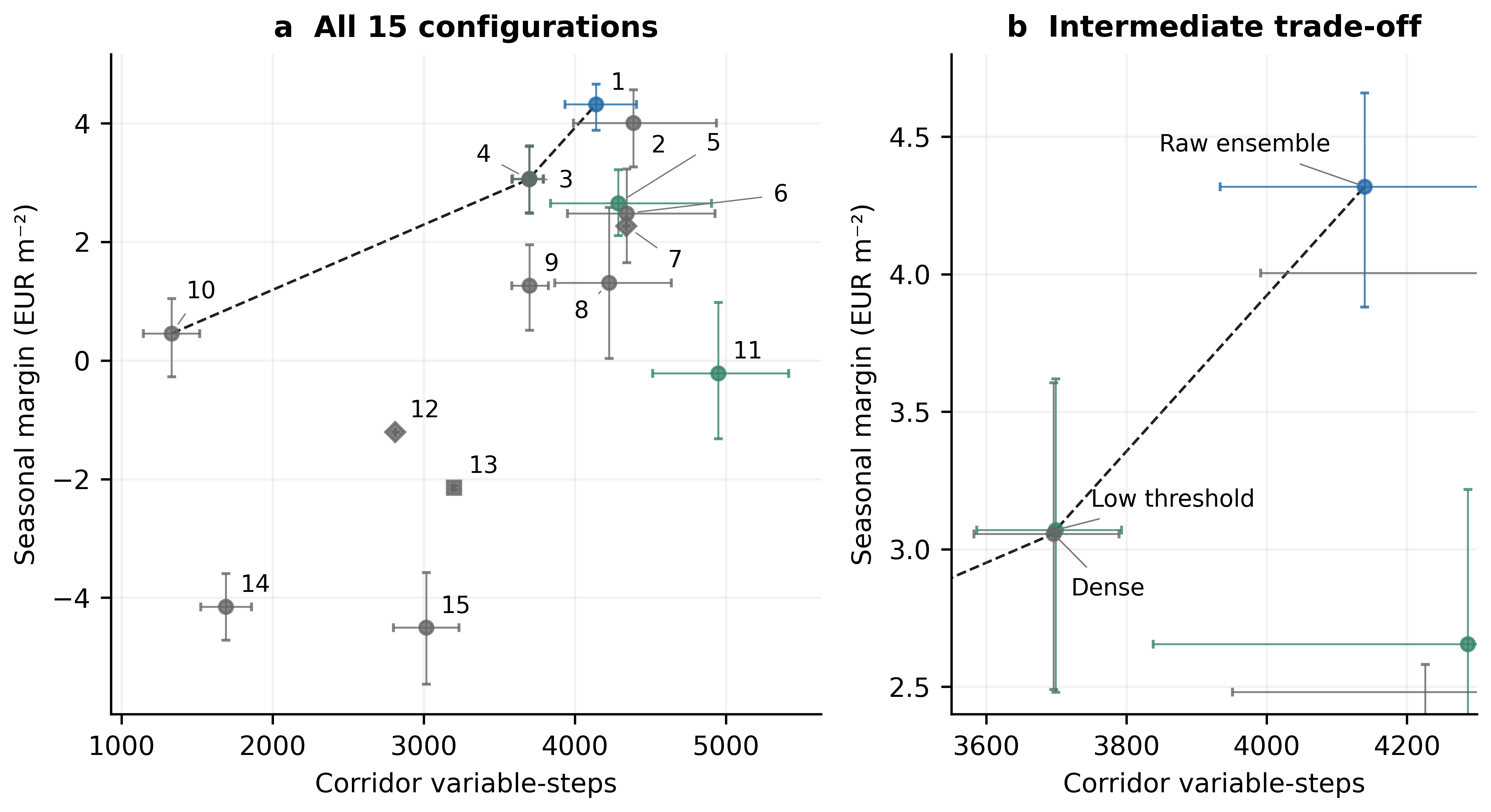
On all 80 common seed–year coordinates, the exact full-season point front contains PPO, dense intermediate, low-threshold intermediate and raw ensemble. Dense with on-policy refitting is not on this point front after completion. Dense and low-threshold controllers remain near-coincident, and their practical distinction depends on the reported tolerance. Bootstrap membership frequencies quantify seed uncertainty conditional on the recorded weather. Seven dense-refitting coordinates in the baseline series span three identification seeds (6, 12 and 17). A crosswalk links their scalar outcomes to corresponding conditions in the primary-environment cohort, whose fitted models, forcing and full trajectories have separate identifiers. The front uses the complete primary cohort.
At the common fitting recipe, the ensemble library sequence gives +4.32, −0.21 and +2.65 EUR m−2 for raw, intermediate and full physics. Economic damage is therefore non-monotone in the number of physical additions: the intermediate library is worse than both neighbours, although conditioning and free-running prediction worsen towards full physics. This contrast cannot be explained by a monotone conditioning-to-margin relation. The low-threshold alternative is evaluated separately because it changes the fitting recipe.
Aggregate corridor counts also conceal different excursion magnitudes. In the baseline-series comparison, raw ensemble spends 453.3/564.8/14.4 h outside the temperature/humidity/CO2 ranges, with conditional excesses 1.02 °C, 1.96 percentage points and 1244 ppm. PPO has shorter durations, 163.7/165.7/3.0 h, but larger temperature/humidity excesses, 1.65 °C and 2.73 points, and only 61 ppm CO2 excess. Shorter duration is not automatically smaller severity. The full-primary-cohort component measurements are in Table S4; baseline measurements are given in Table S36.
Full-state continuations retain the raw ensemble’s higher combined margin among the principal sparse configurations. With the common stock policy, 120-day means are +3.96 for raw versus +2.87 EUR m−2 for low-threshold; with the common tuned policy they are +1.41 and +0.33. All 2096 additional segments complete in the labelled full-parent cohort. This establishes sensitivity to later productive effects in the chosen continuation policies, not an optimal liquidation value for arbitrary terminal crop states.
Uncertainty is at the seed level with weather matching retained. A deterministic heuristic has no stochastic seed interval; the raw-versus-PPO comparison uses independently trained seed samples. The full-season point front and bootstrap memberships are not interchangeable: frequencies in Table S20 quantify sensitivity to sampled seeds and the declared practical tolerances, not probabilities that a controller is agronomically preferable.
3.4. Additional Weather Seasons and Controlled Forcing Interventions
The added priced 2014–2017 comparison retains the raw ensemble’s higher seasonal mean compared to full physics in all eight evaluated years and low-threshold in seven. Across the eight years, their mean raw-minus-comparator differences are +1.95 and +2.17 EUR m−2, respectively. The 2021 reversal remains: the raw-minus-low-threshold gap is −1.81 EUR m−2. Seasonal seed intervals and leave-one-year analyses are reported separately from the descriptive year-resampling summaries.
The fixed-initial-state weather factorial supports a thermal explanation of the 2021 reversal inside this simulator (Figure 3). At horizon 20, replacing all three forcing components by their 2020 values changes the raw-minus-low-threshold gap from −1.81 to +2.85 EUR m−2. The +4.66 change is allocated as +5.14 to temperature, −0.63 to radiation and +0.15 to humidity, averaged over intervention orders. These allocations include interactions; they are not independent additive weather effects or samples from an observed joint climate distribution.
Figure 3.
Order-averaged temperature, radiation and humidity contributions to the raw-minus-comparator margin-gap change for recipient 2021 at horizon 20. Every cell has the same complete 28-state initial vector. The contributions include shared interactions and sum to the joint gap change; labels show baseline and joint gaps. Both recipient years, training-selected horizons, all seven factorial effects and uncertainty are retained in Table S7 and the data.
The 2014–2017 default-objective experiment uses eight seeds, while the priced experiment uses 20 and includes all four principal sparse configurations. Their objectives and budgets remain separate. The complete forcing factorial fixes the recipient initial state and includes all interactions. The default-reset weather swap remains an initialisation-sensitivity check, so a change caused jointly by forcing and crop initialisation is not assigned to temperature alone.
3.5. Actuator-Pathway Survival and Tests of the Boiler Mechanism
The baseline one-factor experiment first associated direct boiler-term survival with the non-monotone library contrast. Degree, denoising, estimator and threshold 0.05 were fixed, and a 17-feature refit tested a specific compensation hypothesis. Figure 4 and the following calculations describe that baseline series; the primary-environment coefficient extension is identified separately. Baseline-series margins of +4.32/+0.28/+2.75 are not pooled with the primary-environment sequence of +4.32/−0.21/+2.65 EUR m−2.
Figure 4.
Baseline feature-library and actuator-pathway comparison. Feature-library choice under open- and closed-loop criteria. Panels (a,b) use the degree-one undenoised fits under the two sparse estimators, 40 per library; open markers in (a) are the fits that fail the divergence gate of 0.05. (a) One-step against 24 h rollout RMSE: the two criteria order the libraries oppositely. (b) The same two metrics against the regression condition number, which orders the open loop monotonically. (c) Four-season simulated margin against boiler-term survival, for the three nested libraries and the 17-feature deletion probe; vertical bars are seed-level standard errors and horizontal bars Wilson 95 % intervals. The nested three differ in nothing but the feature library and the fourth drops one bilinear term, so survival orders these four and does not rank controllers that differ in more than that. (d) The identified boiler coefficient of each replicate against the sparsity threshold, one fit per replicate, with the heavy rule at the median of the survivors. These baseline-series results are reported separately from the primary full-season cohort in Table 3. In panels (b,c), blue denotes the raw library, gold denotes the intermediate library without cross terms, and orange denotes the full-physics library. In panel (c), green denotes the 17-feature library obtained by removing the temperature–boiler interaction term from the full-physics library.
The bilinear-detour hypothesis made a testable prediction. The candidate explanation held that the middle library has enough collinearity for the threshold to destabilise the direct boiler term, while the full library, worse conditioned still, keeps the bilinear term as a detour able to take over the heating pathway once the direct one is cut. That account predicts that deleting exactly the bilinear feature from the 18-feature full library (17 of 18 features, and essentially all of the collinearity, unchanged) should collapse the truncated library onto the middle one, with boiler survival near 0.15 and margin near +0.28 EUR m−2 rather than near +2.75 and 0.55.
The 17-feature library without the temperature–boiler interaction does not collapse (Table S29, fourth row pair). It keeps the full library’s conditioning (κ = 52.3 against 53.4, mean over 20 refits), its open-loop instability (median rollout 24.2 °C, divergence 0.084, both under the ensemble estimator) and its closed-loop level: +2.11 EUR m−2 under the ensemble estimator and +2.28 under STLSQ. Relative to frozen intermediate, the ensemble deletion model has a mean four-year seed effect of +1.83 EUR m−2 [0.67, 2.99], with 16/20 positive seed means and pHolm = 0.036. Neither deletion arm separates from full physics under the four-test seed-level Holm analysis (pHolm = 0.307 for both estimators). Table S44 gives all four contrasts and descriptive seed intervals. Boiler-term survival moves only part of the way down, to 0.40 (8 of 20 replicates; exact McNemar test against the full library p = 0.55), and nowhere near the predicted 0.15. The result rejects the proposed detour as a sufficient explanation; it does not identify which feature correlation causes pathway loss.
Figure 4d shows how far the surviving coefficients sit above the cut. Where the direct boiler coefficient survives, its standardised magnitude lies between 0.06 and 0.08 in the raw library (median 0.069, 11 of 20 replicates) and between 0.06 and 0.07 in the library without cross terms (median 0.061, 3 of 20), just above the threshold of 0.05, whereas the full library splits: 5 of its 11 survivors lie between 0.05 and 0.07 and 6 between 0.14 and 0.19 (median 0.143). A coefficient the threshold removes is stored as exactly zero, so the panel says nothing about how far the cut terms fell short.
The baseline 2020 paired edit copies the direct boiler coefficient from the same-seed low-threshold donor, holding other coefficients fixed. Survival rises from 0.15 to 1.00. Under priced weights, 16/20 effects are positive (p = 5.9 × 10⁻⁴; Holm p = 0.0018 over four primary edits), but the median gain is +0.21 versus mean +1.92 EUR m−2. A few large effects therefore dominate the mean. The default-objective median is +3.05, about 14 times larger; objective and execution environment both differ between those waves. Knock-out has zero median and is not significant, with the term already absent in 17/20 baseline seeds. The separate low-threshold cross-term edits are non-significant and two of three estimates reverse sign between objectives. They do not test the detour because their baseline retains the direct boiler term in all 20 seeds.
The baseline 13-level threshold sweep (Figure 5; Table S30) loses the boiler term between thresholds 0.03 and 0.06: survival falls from 0.95 to zero. Levels at which at least one seed retains the term average +5.77 EUR m−2 against +3.47 for levels at which none does, under the priced objective (+3.46 vs. +2.77 under the default). The separation is not monotone under either objective: the worst retaining level (4.04, priced) is below the best non-retaining one (4.61), so EPI is not monotone in boiler-term survival within this library, as it is not across libraries. The priced wave has higher EPI at every one of the 13 levels (+0.34 to +2.95) and lower violations at each. Because thresholding changes multiple coefficients, this sweep is not an isolated causal test of the boiler pathway; the paired edit provides that separate comparison.
Figure 5.
Baseline threshold and 2020 coefficient-edit experiment. Sparsity threshold and boiler-term analysis with the intermediate feature library, season 2020 (n = 20 per condition). The 13 threshold levels are drawn evenly spaced rather than to scale, so that the collapse between 0.03 and 0.06 is visible; every level is labelled. (a) Mean margin with SD. (b) Boiler-term survival on the same threshold grid, with the survival of each closed-loop controller of the priced pool marked on the right-hand strip, one fit per replicate. (c) Seed-paired coefficient knock-in under each stage cost; grey lines join the same replicate, the heavy tick is the median and the open circle the mean. The knock-in is positive in 17 of 20 replicates under the default stage cost (p = 3.2 × 10⁻⁴, mean +2.52) and in 16 of 20 under the priced one (p = 5.9 × 10⁻⁴, mean +1.92); the primary four-test Holm adjustment for knock-in and knock-out under both stage costs gives 1.3 × 10⁻³ for the default cost and 1.8 × 10⁻³ for the priced cost. The complementary knock-out is null under both stage costs, with median +0.00 and one positive replicate of 20 in each, because the coefficient it removes has mostly been cut already. The threshold sweep and cross-term edits are exploratory. The separate four-season extension appears in Figure 6. The yellow shaded regions in panels (a,b) highlight the threshold range λ = 0.03–0.06, over which boiler-term survival declines to zero. The dotted vertical lines mark the frozen-recipe threshold λ = 0.05. The shaded bands in panel (a) represent mean ±1 SD for the corresponding stage cost. The shaded boxes in panel (c) show the interquartile range (25th–75th percentiles) of the seed-paired knock-in effects.
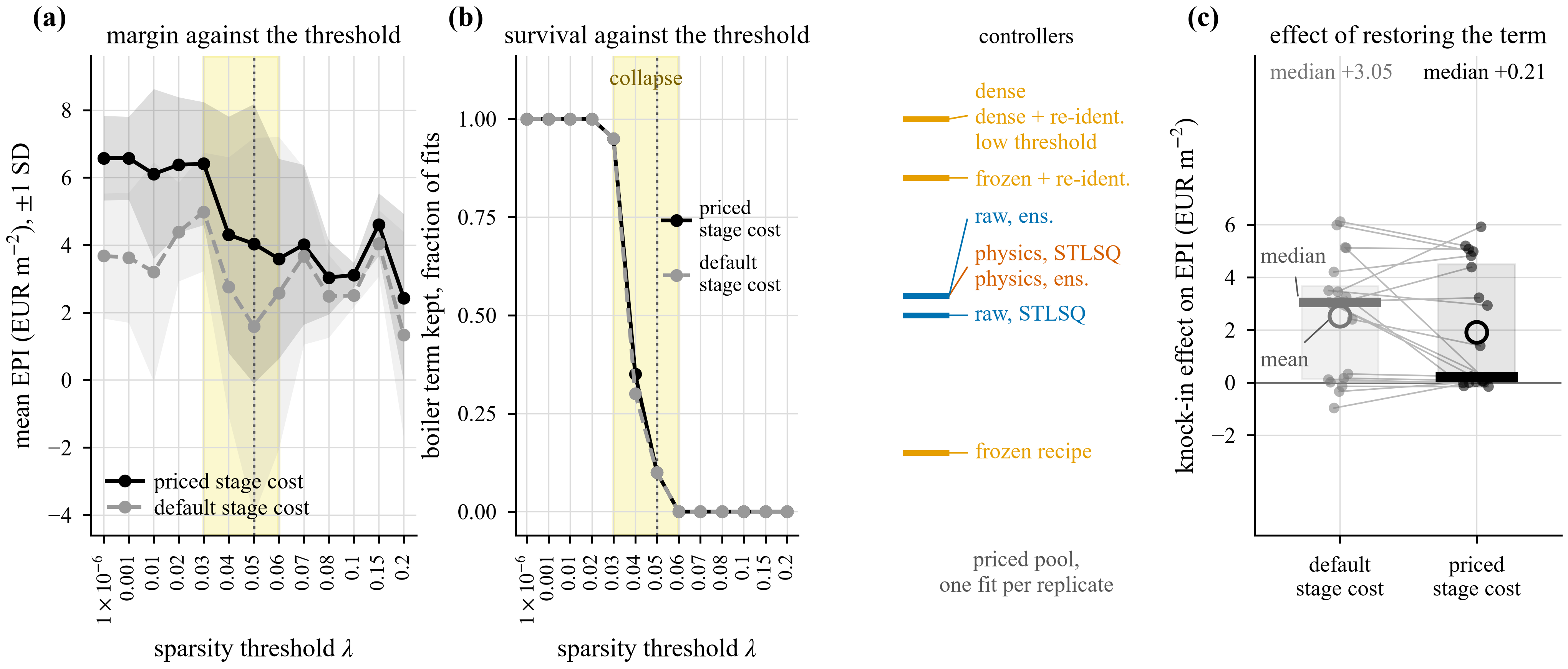
Table S31 decomposes EPI over the four test seasons by library and by whether the boiler term survived, now over all three libraries. Within the intermediate library, the gap is +2.34 EUR m−2, and within the raw library, it is +1.13; within the full-physics library, it is −0.22 and not significant. Raw with its direct term dropped (+3.48) still exceeds intermediate and full physics with it kept (+2.36 and +2.52). Across seeds, the association is significant only for intermediate physics (p = 0.0015 priced; 0.0006 default), not raw (0.136; 0.316) or full physics (0.178). Survival is fixed across a seed’s weather years, so the effective stochastic unit is the fitted seed, not 80 seasonal rows. The groups also mix fitting recipes: their differences are observational and cannot replace the within-recipe intervention, whose priced median is only +0.21.
The extended paired edit of the frozen intermediate model under priced weights raises the four-season seed-mean margin by 1.78 EUR m−2 [1.10, 2.45], with Holm p = 0.0039 in the 12-test extension family (Figure 6). Effects differ across recipe, objective and edit, and all 12 are shown. This is intervention evidence for a specified coefficient at the evaluated conditions, whereas associations between survival and unedited library performance remain observational.
Figure 6.
Four-season paired boiler-coefficient intervention effects for three recipes and both objectives. Points are means of 20 four-year seed effects; bars are descriptive 95% intervals. Filled symbols have Holm p < 0.05 in the declared 12-test extension-margin family, while open symbols do not. Default denotes the non-price-aligned objective. The 2020 four-test primary family is described separately in Section S21.
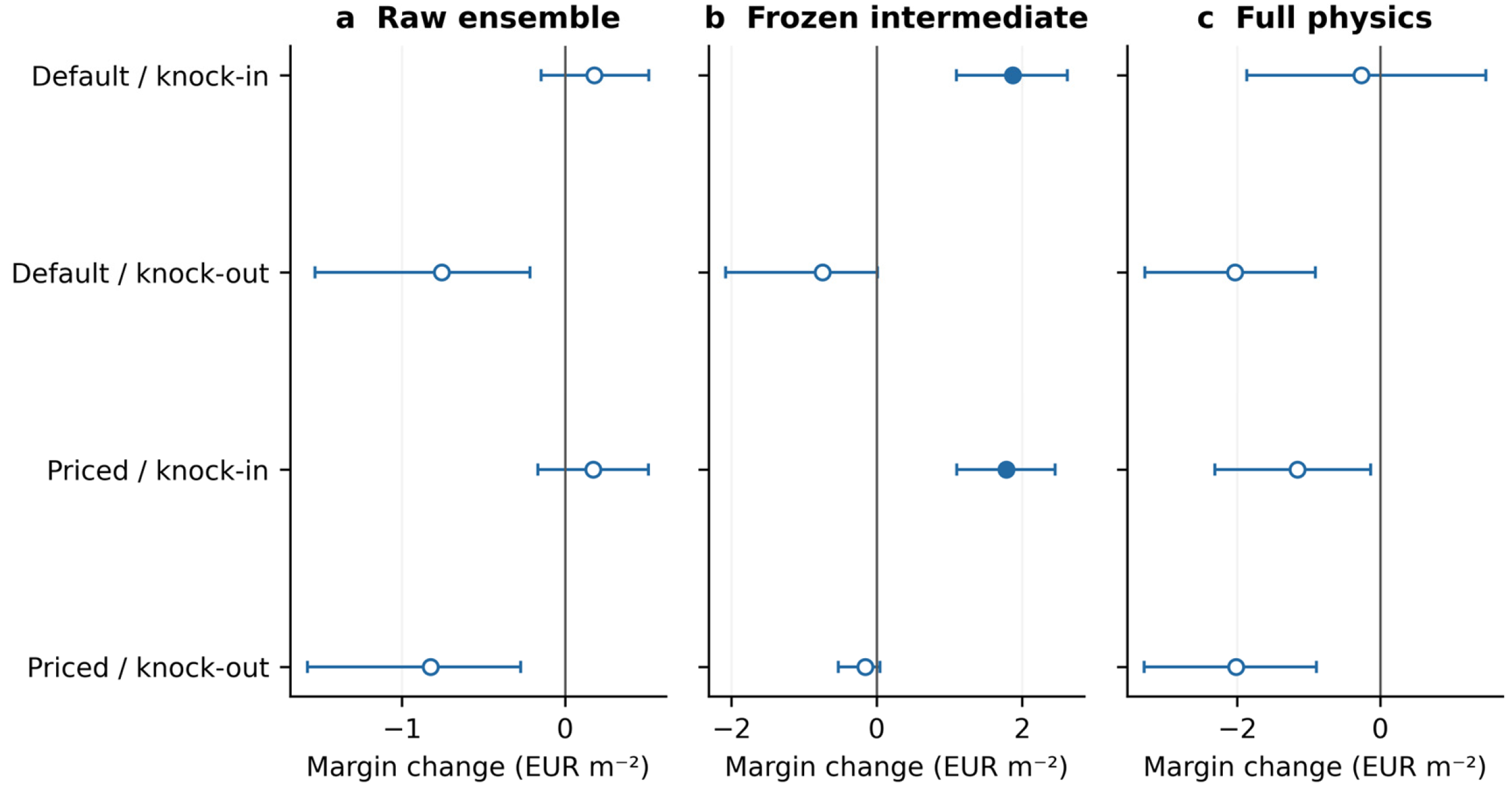
The extended intervention retains the same paired-fit construction over three recipes, two objectives and four seasons. Its 12-test margin family is separate from the 2020 four-test family. Copying one stored coefficient holds the remaining model fixed; changing a candidate feature and refitting does not. A result for one edited coefficient therefore cannot explain the complete library contrast or establish an isolated seasonal profit effect for every actuator.
The complete audit contains 14,400 state–actuator distribution records for all three states and six controls. A standardised direct coefficient alone is not a native-unit response: scaling and state–input products enter the local derivative. Heating and CO2 injection have their stated local checks, while ventilation can change direction with inside/outside conditions. These measurements complement the full-season coefficient intervention; fault experiments additionally change the simulated plant and supervisor.
3.6. Alternative Explanations and Solver Reliability
The unmodified main cohort contains 987 complete trajectories, 41 numerical simulator stops and 20 exception-cap stops. The stable numerical formula completes the 41 former simulator stops without removing state guards. The raised-cap benchmark then completes the remaining 20 planner seasons. Across the primary-environment campaigns, the audit covers every unique incomplete condition, not only the seven dense-refitting coordinates. Unmodified stops, exact-repeat evidence, completion outcomes and 96-step stop windows remain separately accessible. The main early-stop conditions and completion protocols are summarised in Table 4.
A zero caught-exception count does not mean optimiser convergence. In the full cohort, neural MPC records 435,260 unsuccessful optimiser statuses; eight sparse configurations also return unsuccessful statuses, although none catches an exception. Returned actions are still applied. Table S3a reports controller-wise distributions, fallback frequencies and available NLP residuals; the latter have mixed constraint units and do not certify climate safety. Table S12 compares fixed-command, previous-action and rule-based planner fallbacks. The raised cap remains a separate protocol choice.
A two-seed exception-cap check is supplied alongside the 20-seed comparison. The 20-seed 2022 comparison raises the exception allowance from 100 to 100,000 without changing the per-step CEM search. All 20 runs reach 5760 steps, averaging −0.64 EUR m−2 and 118.85 fallback actions. With the same large allowance, previous-action and rule-based fallback yield +0.28 and +0.40 EUR m−2, respectively, and complete all 20 seasons each. The 2020 fallback comparison is also retained. This tests exception tolerance and fallback choice, not an increased per-step planning-search budget or a globally optimal full-model policy.
Prediction error along the operating trajectory is small. Replaying both surrogates with the intermediate feature library along the full-model planner’s own closed-loop trajectory (5760 steps, 5 seeds, season 2020) gives one-step temperature RMSE of 1.89 ± 0.09 and 1.82 ± 0.04 °C (R2 = 0.82 and 0.83) and 24 h rollout RMSE of 2.62 and 2.49 °C, with zero diverging rollouts out of 100 at every horizon. The same frozen recipe measures about 10.5 °C on the excitation data of the ladder—roughly four times larger. The surrogate is far more accurate along a smooth closed-loop trajectory than on PRBS-excited identification data, and the ladder number is not its error in operation.
The baseline default-objective horizon check improves all four tested variants when shortening 20 steps to 8: the raw gain is +0.29 EUR m−2, versus +1.30 to +2.12 for intermediate variants, with no rank change in that subset. The larger benefit for poorer free-running models is consistent with accumulated prediction error. Full physics was absent, so the argument cannot cover it. A separate single-controller sweep gives +6.11, +5.13, +3.63 and +0.91 at horizons 8, 12, 20 and 30, with SD increasing from 0.87 to 4.03. These baseline checks are distinct from the training-only priced selection in Section 3.9.
The bootstrap draw of the ensemble optimiser is a secondary source of variation. Resampling the ensemble draw (6 seeds × 6 draws × 4 seasons, default objective) leaves the raw-library controller leading in 32 of 36 seed × draw cells (0.89). Its spread across draws within a seed averages 0.26 EUR m−2 against 1.11 for the frozen recipe and 2.04 for the re-identified variant, but this average conceals a concentrated adverse case. Five raw seeds have a spread of at most 0.25; one contributes 1.18, exposing one adverse basin. This wave disagrees with the canonical 20-seed/10-draw wave on frozen-recipe survival and leadership, so the waves remain separate and draws do not become independent identification cases.
Table 4.
Main conditions that stopped early in the unmodified common-environment campaign. Originally complete trajectories remain unchanged. Full results are separately labelled numerical-completion or raised-cap variants. Simulator stops are not called biological termination or proven safety failures.
3.7. Adaptation Safety Guards and Fault Supervision
The following adaptation and guard experiments use the default objective over 2021–2023 in the baseline series. Their recorded season lengths are preserved. The displayed row-level p-values describe repeated seed–draw–year records; these records do not constitute independent model fits for primary inference. The baseline outcomes are reported separately from the primary full-season cohort.
Three adaptation modes were compared on the three harder seasons (2021–2023) with 20 seeds × 10 ensemble draws per condition, 600 runs each, under the default objective. On-policy re-identification (the surrogate is rolled out in closed loop, the visited states are appended to the training set and the model is re-estimated, with no expert queried, so this is not Dagger [37]) gives −0.39 EUR m−2 against −1.58 for the static model (paired Δ = +1.19, median +0.40, 380/600, p = 5.0 × 10⁻¹⁶) and reduces violations from 5424 to 4654. Recursive coefficient adaptation by extended Kalman filter is harmful: −2.95 EUR m−2 (Δ = −1.36 against static, p = 7.4 × 10⁻¹⁴) with 234 of 600 seasons terminating early. All three are net-negative in absolute terms because 2020, the favourable season, is absent from this block.
The Mahalanobis-distance safety guard [44,45] lowers the mean margin and raises the violation count. Guarded runs average −2.59 EUR m−2 against −1.91 unguarded runs. The paired mean difference is −0.69, but the paired median is +0.19 and the guard is better in 335 of 600 pairs (p = 0.0047). The median margin is −2.20 EUR m−2 with the guard and −2.57 without it, so mean and median favour different policies. Both statistics are reported, although the early stops limit this comparison. Violations are worse under the guard (+430 steps, worse in 529 of 600, p = 5 × 10−85), and 179 of 600 guarded seasons terminate early. Restricted to completed seasons, the margin difference is −0.33 and not significant (p = 0.081). The underlying detector is weak: the area under the ROC curve is 0.663 ± 0.042 for the distance statistic and 0.627 ± 0.058 for ensemble spread [46], barely above chance. The guard’s activation count was never recorded, so the natural explanatory variable is unmeasured.
Early-stop treatments qualify these baseline-series contrasts. On-policy refitting has complete pairs and retains its +1.19 EUR m−2 mean gain. For EKF, the mean difference versus static changes from −1.36 as recorded to −0.89 over 366 complete pairs; rate scaling gives −1.57. For the guard, it is −0.33 over 421 complete pairs, versus −0.69 as recorded and −0.79 after rate scaling. Excess guard violations persist under each treatment. Rate scaling is a diagnostic of accumulated outcomes, not a simulated continuation. Table S42 retains the full paired counts and both outcomes.
The residual-based fault supervisor, in contrast, is beneficial (Table S32). It improves the margin under all six injected faults (paired over 20 seeds, all p ≤ 1.7 × 10⁻³, and unchanged in that bound under Holm correction over the six) and collapses the dispersion from SD = 1.16–5.48 to 0.29–0.39: it reduces dispersion more than it raises the margin. Violations fall sharply (9131 to 5292 under a dead vent; 5198 to 2660 under a stuck boiler). Two faults remain net-destructive even when supervised. With the lamps dead, the supervised fallback (+6.33) outperforms the nominal fault-free controller (+3.63); this contrast also changes modelled crop revenue and several resource costs.
Fault gains combine crop response with several resource costs. In the dead-vent experiment, supervision raises baseline-series revenue by 5.96 and reduces total cost by 12.33 EUR m−2, explaining the +18.28 margin change. With lamps dead, the supervised margin exceeds the nominal one by +2.70: revenue is +2.15 and total cost −0.55, while electricity alone falls by only 0.17. This does not identify a pure lighting effect or prove that nominal lighting is excessive. All 260 fault/reference seasons complete; the revenue-minus-cost identity holds to rounding precision (Tables S32 and S43 and the paired accounting data).
3.8. Sensitivity to Design Parameters and Fixed-Trajectory Prices
The coefficient stress test remains strongly sensitive after full-season completion. At 20% noise, 68 of 80 perturbed models pass the local screen. The priced mean margin is −10.66 EUR m−2 across all 80 and −11.26 in the passing subset. The all-model median is +1.70 EUR m−2, so the mean reflects a large adverse tail rather than a uniformly negative response. A local sign/bounds screen therefore does not remove the poor tail or guarantee favourable crop outcomes. These intentionally perturbed models are a stress test, not ordinary controller operation. Separate resource and climate multiplier effects, all baseline observer/guard results and their completion treatments are retained in the Supplementary Information.
The baseline coefficient-perturbation experiment and the completed both-objective extension retain distinct models, sample sizes and numerical protocols. Their adverse tails are scientific outcomes rather than a reason to omit failed unmodified seasons. The local sign/bounds screen admits models that later perform badly; it cannot certify the seasonal feedback loop. Threshold sensitivity is developed with the mechanism in Section 3.5, while independent resource/climate multipliers and plant discrepancies are reported separately.
The baseline 3 × 3 price exercise revalues the same ten fixed policies. It measures accounting sensitivity without changing their actions, and its controller subset omits the two raw-library policies. In that fixed-trajectory grid, the stock heuristic leads at six price pairs and dense on-policy refitting at three. It cannot establish the ranking after economic retuning. The price-dependent selection in Section 3.9 instead changes policies using training-season crop margins and includes the raw and full-physics alternatives; Figure S4 shows the baseline valuation.
3.9. Training-Selected Horizons and Price-Dependent Policies
Training selects horizon 12 for raw ensemble and horizon 8 for the other three principal configurations. Rescoring the completed training seasons preserves all four horizon choices and all 36 price-dependent choices. Test mean margins at the selected horizons are +4.42 EUR m−2 for raw and +3.77 for low-threshold (Table 5). Their difference is 0.65, with a descriptive seed interval [−0.12, 1.34] and Holm p = 0.058 across the three tuned-library margin comparisons. The mean order survives this declared tuning grid, but separation from the nearest alternative is not established at 0.05. The finite horizon/weight searches remain under-optimised relative to an unrestricted policy search.
Table 5.
Training-selected horizon test results. Selection uses 2018–2019 only; test outcomes cover 20 seeds × 2020–2023. The difference column compares each selected policy with its horizon-20 reference; Holm adjusts those four within-controller margin tests. The separate three-test comparison among tuned libraries is reported in the text and Table S18.
After training-only price-dependent selection, raw ensemble has the largest mean among the four principal sparse configurations at all nine price pairs (Table 6; Figure 7). At nominal prices the means are +5.33 and +4.48 EUR m−2 for raw and low-threshold, a difference of 0.85 [0.07, 1.62]. Holm p = 0.123 in the 27-test library-margin family. Raw also has greater corridor exposure than low-threshold. The independently retuned heuristic has a higher mean than raw at three price pairs. These are finite-search comparisons, distinct from the retained retrospective revaluation of fixed baseline-series trajectories; selection frequently reaches the resource-weight grid boundary.
Table 6.
Mean margin after price-dependent policy selection, EUR m−2. Each MPC cell contains 80 complete trajectories; the independently retuned heuristic has four deterministic test seasons. Choices are frozen on training years. Largest mean does not establish Holm-adjusted superiority over every alternative.
Figure 7.
Price-dependent policy comparison based on actual selected control policies. Cells show raw-ensemble minus comparator mean margin, EUR m−2, after choices on 2018–2019 and evaluation on 2020–2023. Each MPC cell has 80 full trajectories; the independently retuned heuristic has four deterministic seasons. These are mean differences, not significance states. The 27 library-margin tests and nine reference-margin tests use separately declared Holm families. The nominal raw-minus-low-threshold Holm value is 0.123.
3.10. Plant Crop-State and Numerical Robustness
Raw retains the highest mean among the four configurations in all four declared plant discrepancies. Controlled OS/libc comparisons give identical refitted coefficients, zero corridor-count drift and a maximum absolute margin drift of 1.8 × 10⁻¹⁵ EUR m−2. This narrow portability result does not establish portability across arbitrary libraries or numerical harnesses. Common-reference coverage remains imperfect: complete range and joint-distance diagnostics are reported for all main trajectories, not interpreted as proof that every controller operates inside its own training support. Selected robustness results are summarised in Table 7.
Table 7.
Selected robustness results. Complete conditions, both objectives, negative results, uncertainty and protocol identifiers are retained in Tables S7–S19 and the data. These comparisons do not establish global policy optimality or field validation.
The continuation, plant-map and portability checks address different uncertainties. Full-state handovers preserve later productive effects under two common policies. Plant-only perturbations leave the nominal identified controllers fixed and test discrepancy inside the same greenhouse–crop model. Controlled OS/libc changes test a narrow numerical factor. None supplies an independently calibrated crop model or a field trial, and the nominal controller order must be read with the weather and price reversals that are already reported.
4. Discussion
4.1. Physical Features Actuator Pathways and Non-Monotone Effects
The comparison supports a concrete identification-for-control lesson: improving one-step prediction through additional physical transforms can worsen free-running dynamics and need not improve the resulting feedback policy. The transforms reuse measured variables, and conditioning, sparse thresholding and actuator pathways can change together. The effect is measured within the three tested sparse libraries; it is not a claim that physical knowledge or mechanistic modelling generally harms control. Same-recipe ensemble comparisons isolate library choice more cleanly than comparisons involving a different threshold or estimator.
Full physics outperforms intermediate physics despite worse conditioning and more terms. The raw-without-boiler counterexample also makes pathway survival an incomplete explanation. The unsuccessful detour test refutes a specific compensation hypothesis without identifying which feature correlation removes the direct term. Thus, the screen identifies the leading library rather than the entire economic order, and the stored-coefficient intervention establishes its specified effect rather than the causal effect of adding a whole library. The one-factor contrasts, survival splits and paired edits answer distinct scientific questions.
4.2. A Practical Workflow for Control-Oriented Surrogate Selection
Three recommendations follow for practice. First, screen candidates open-loop on (i) free-running multi-step rollout error at a horizon no shorter than the one the model will be used at and (ii) the fraction of rollouts that diverge. Report the one-step error and conditioning as diagnostics, but do not use improved one-step accuracy as evidence that feedback will improve. Here, the 96-step screen is a 24 h stress test against a five-hour reference controller. It is much cheaper than running a season for each candidate, although no hardware-independent speed-up is claimed. The audit is retrospective, so the thresholds require prospective testing on new data.
Second, after sparsification, read the fitted coefficient matrix and confirm that every actuator the controller is allowed to move still has a surviving path to the states it is meant to move. Use native-unit equations and sampled state–input Jacobians, not merely a nonzero standardised coefficient. If a pathway is lost, a lower threshold, a different basis or a protected coefficient is a candidate remedy. The present study tests threshold changes, feature deletion and specified boiler edits; it does not validate every such remedy or require one unconditional ventilation sign.
Third, tune the admissible controller on training seasons and assess full-season margin together with corridor duration and severity. Multi-step screening narrows the candidates; it cannot reproduce every closed-loop rank or select an economic optimum without a control trial. Training-selected horizons and price-dependent resource weights test whether a baseline was under-optimised, while independent seed and weather checks establish the limits of the resulting comparison.
The retrospective numerical rule selects raw/STLSQ, whereas raw ensemble has the highest reference-setting mean margin. Reporting both prevents selecting whichever seed or estimator gives the best test return. A physically motivated feature should be entered as a candidate in the ladder and then judged by the open-loop screen like any other candidate.
Prediction error also depends on the excitation and evaluation year. In the baseline replay, the frozen recipe had 2.62 °C 24 h temperature error on the planner trajectory versus 10.50 °C on PRBS data. In the held-out block, intermediate physics had median 16.9 °C on 2018 and 2.7 °C on 2019. The joint-coverage and three-state held-out tables expose these differences rather than treating a single in-sample score as its deployment error. In the baseline fit-2018/evaluate-2019 block, intermediate has median 24 h temperature RMSE of 2.687 °C versus 2.722 °C for raw; this small descriptive reversal is not evidence of statistical superiority.
4.3. Sparsity and the Library Effect
Term count does not explain the library order. The baseline threshold sweep in Table S30 has non-monotone intermediate levels but worse margin and greater corridor exposure at its sparse endpoint. Across the baseline ensemble library series, active terms rise 20.2 → 28.25 → 37.2 while margins change +4.32 → +0.28 → +2.75 EUR m−2. The middle model is neither the sparsest nor the densest. The baseline non-significant raw-ensemble versus STLSQ test also does not establish equivalence. The primary-environment replication and audit keep model-size effects separate from estimator uncertainty.
4.4. Sensitivity to Reference Tuning and Economic Weighting
Two benchmarking safeguards materially changed the comparison (Table S35, Figure S5): tuning the agronomic reference and aligning MPC resource weights with the prices used for evaluation. The apparent advantage of the raw-library controller over it falls from +5.54 to +2.06 EUR m−2. Aligning resource weights reduces the baseline raw-minus-intermediate gap from +3.66 to +1.23. These baseline-series effects (Table S35 and Figure S5) cannot be assumed to reproduce the primary-environment contrast, but they explain why tuning and objective scope are necessary parts of the scientific comparison.
The term economic MPC is used here for a resource-cost component in a climate-control objective. The outer training search uses simulated crop margins, but it selects among a finite family of climate policies; it does not introduce biomass prediction into the inner programme. Crop-profit optimisation with an explicit crop state is a different controller formulation. The default-objective and fixed-trajectory price calculations remain informative within their stated scopes, and the price-specific trajectories address a stronger robustness question.
Mean rank and statistical separation must also be distinguished. Horizon tuning and price-dependent selection retain raw’s mean lead among the four principal configurations, but neither establishes adjusted separation from the closest low-threshold alternative in every setting. PPO and the intermediate configurations offer different climate exposures, and a retuned heuristic wins at some prices. These results support a conditional margin–climate choice, not a universally preferred controller. Practical tolerances require agronomic justification before deployment; the present tolerance grid is a transparent sensitivity analysis.
Terminal crop state is another boundary condition rather than an omitted sale of standing fruit. Fruit-growth revenue has already been counted. Full-state handovers test later effects under two common policies, preserving raw’s higher mean within that design. Different crop ages, continuation weather, management policies or costs could alter the comparison. The same distinction applies to plant-map and weather interventions: they identify responses of a declared simulator, not independent field validation.
At nominal prices, the completed training-selected policies yield +5.33 and +4.48 EUR m−2 for raw and low-threshold, with Holm p = 0.123 in the 27-test library family. Raw has the largest mean among the four sparse configurations throughout the tested price grid, while an independently retuned heuristic wins at three prices. Economic weights and the reference policy therefore affect the decision even when that within-MPC mean order persists. The selected grid boundary and unequal cross-family training budgets remain explicit limits [47].
4.5. Relation to Prior Work
These results connect identification for control [18,19,20,25,26] with objective mismatch in model-based reinforcement learning [21,22,23,24]. Prediction likelihood or one-step error is not the control criterion. The completed retrospective audit and closed-loop comparison both favour the raw library, while multi-step scores still fail to order every alternative. Conditioning measurements agree with the motivation for reweighted or balance-guided sparse regression [29,30,31], but the further conditioning-to-profit relation is non-monotone. Library optimisation based on recursive prediction [17] addresses the same modelling issue through a different procedure. Bagged ensembling [13] does not by itself remove library sensitivity, and a non-significant estimator contrast is not an equivalence result. Unlike greenhouse comparisons that vary the controller on a fixed model [6,14,15,16], this experiment tests the surrogate library as a factor and then checks its tuning, economic weighting and actuator responses.
This study also contributes to simulation-based research on greenhouse climate control. Xu et al. used a mechanistic greenhouse–crop model to compare open- and closed-loop optimal control and reported simulated yield and profit [7]; Wen et al. combined an experimentally fitted photosynthesis surrogate with multi-objective regulation of light and CO2 [8]; and Ećim-Đurić et al. coupled transient building simulation with an ANN after comparing modelled and measured greenhouse temperatures [9]. The present contribution differs by holding the mechanistic greenhouse fixed and treating surrogate selection itself as the experimental factor. It also provides a lower level of empirical evidence than studies that operate controllers on a crop, such as the eight-week reinforcement-learning irrigation evaluation of Padilla-Nates et al. [48]. Accordingly, our results support model and controller design choices for subsequent testing; they do not establish agronomic efficacy in a physical greenhouse.
4.6. Limitations and External Applicability
The paired coefficient edits establish effects of the specified edits across the tested recipes, seasons and objectives. They do not assign the entire library contrast to one boiler term. Structural error and unmeasured actuator dynamics remain separate uncertainties.
Weather, economic weighting, model structure and actuator-pathway identification are the principal uncertainties measured here. Weather can reverse a seasonal rank; economic weighting changes the selected policy and the reference controller; coefficient perturbations create a poor tail even after local screening; and finite optimisation/fallback choices alter realised outcomes. Seed intervals do not absorb these uncertainties into one probability statement. The eight-year analysis remains a one-site sensitivity study, while cross-family rankings remain conditional on the unequal but declared training and planning budgets.
The surrogate is spatially lumped and omits unknown time-varying disturbances and actuator-lag states. An adaptive residual model could be added to the climate dynamics and updated from measured prediction residuals, with its effect evaluated under the same resource and corridor criteria. Liu et al. [49] propose a congealed neural architecture that separates a fixed weight component from time-dependent uncertainty in an adaptive tracking problem. Its assumptions and tracking results cannot be transferred directly to this greenhouse MPC. Integrating such a framework, testing additional surrogate architectures and collecting greenhouse measurements are directions for a separate study.
The stable numerical formula was validated on every rejected checkpoint, and affected trajectories were rerun. The full-season cohort combines unmodified complete trajectories and named completion variants. Matched primary-environment replications, full logs and source-bound statistical reproduction support the comparisons. Baseline-series and primary-environment cohorts have separate identifiers. These tests do not establish recursive feasibility, stability or commercial greenhouse performance.
The greenhouse is represented by one site, crop model and planting schedule, without independently observed harvest, grower intervention, pests or wear. Spatial fields, a wind input, actuator-lag states and unknown disturbances are omitted. The full-state continuation and weather factorial strengthen internal comparisons without substituting for greenhouse measurements. Hardware-in-the-loop work and a crop pilot would address those remaining external questions. The baseline negative guard/observer results and the completed coefficient-stress tail also preclude treating symbolic accessibility or local plausibility as safety certificates.
5. Conclusions
Within the GreenLight tomato testbed, one-step and free-running prediction order tested sparse feature libraries differently for all three climate states. The completed transparency audit selects a raw fitting recipe, and the full-season controller comparison retains raw ensemble’s highest reference-setting mean margin (+4.32 EUR m−2). Its 4140 corridor variable-steps contrast with PPO’s +0.45 EUR m−2 and 1330 variable-steps, so economic rank alone does not determine controller choice.
Training-selected horizons and price-dependent policies retain raw’s largest mean among the four principal sparse configurations at all nine tested prices. At nominal prices, its tuned margin is +5.33 versus +4.48 EUR m−2 for the low-threshold controller, without Holm-adjusted separation from that nearest competitor. In I 2021 rank reversal, price-retuned heuristic wins and the four-member full-season Pareto front remain explicit.
Weather interventions, full crop-state continuations, controlled coefficient edits, actuator diagnostics and plant/portability sensitivities support a joint assessment of prediction, interpretation, tuning and realised closed-loop outcomes. They delimit the evidence: coefficient effects are specific interventions, selection is retrospective, and validation is computational. Complete experimental designs, numerical results and supporting calculations are supplied in the Supplementary Information and data. Architecture and field validation remain separate research questions.
The practical outcome is a staged selection workflow: test multi-step dynamics, inspect actuator pathways, and then tune and evaluate the resulting controller over complete seasons. Its scientific basis includes the non-monotone library contrast, the unsuccessful bilinear-compensation explanation and the separation between a recipe chosen by open-loop audit and the controller with the highest observed mean margin. These distinctions preserve the mechanism evidence and its counterexamples within the stated simulation study.
Supplementary Materials
The following supporting information can be downloaded at: https://www.mdpi.com/article/doi/s1, Table S1: Controller definitions for the 15 main configurations and two term-deletion probes; Table S2: Complete three-state degree-one prediction summary; Table S3: Unmodified and completed-cohort outcome treatments; Table S3a: Solver diagnostics for the full main cohort (1048 complete trajectories); Table S4: Full-cohort violation duration and mean per-trajectory conditional excess; Table S5: Horizon selection scores after completion, 40 training seed–year cells per row; Table S6: Training-selected horizon/resource multiplier for each price pair; Table S7: Matched-initial-state weather gap decomposition; Table S8: Mean native-unit one-step input derivatives, averaged over the sampled trajectory distributions; Table S9: All 12 four-season coefficient interventions; Table S10: Coefficient stress test after numerical completion; Table S11: Independent common-resource or common-climate multipliers; Table S12: Planner-cap and fallback sensitivity; Table S13: Common-policy full-state continuations in the completed-parent cohort; Table S14: Controlled OS/libc portability with scientific package files fixed; Table S15: Joint three-state/six-action coverage; Table S16: Weather summaries at exact consumed control coordinates; Table S17: All 54 distinct recipe screens after removing the constrained/SR3 duplicate; Table S18: Raw-minus-comparator margin effects with 20 matched identification seeds; Table S19: Held-out-year errors from 120 fits and 240 fit–evaluation cells; Table S20: All-15-controller Pareto audit on 80 common full seed–year coordinates, including the labelled raised-cap planner; Table S21: Controllers compared; Table S22: Rule-based setpoint search; Table S23: Three benchmarking risks, the safeguards used in this study and the measured sensitivity to removing each safeguard; Table S24: Baseline identification ladder, degree-one configurations without denoising; Table S25: Tuning the rule-based reference with its 16-trial setpoint search; Table S26: Seasonal margin in EUR m−2 and corridor variable-steps for all 15 controllers; Table S27: Comparison against the deterministic tuned heuristic; Table S28: Additional weather years; Table S29: One-factor library comparison; Table S30: Sparsity sweep within the physics_no_cross library, season 2020, 20 seeds per level; Table S31: Mean EPI by feature library and boiler-term survival, pooled over the nine SINDy-MPC controllers and four test seasons; Table S32: Fault injection with and without the residual-based supervisor, season 2020, 20 seeds; Table S33: Coefficient-perturbation sensitivity in the 2020 season; Table S34: The selection reversal, measured on the held-out identification block; Table S35: Sensitivity of the headline comparison to two benchmarking safeguards; Table S36: Baseline-series results: mean time outside each evaluation corridor per run and mean exceedance during steps with a violation; Table S37: Baseline-series results: caught exceptions and fallback use in all attempted runs of the 11 predictive controllers; Table S38: Baseline-series results: seed-level effects of the raw-library ensemble against principal comparators; Table S39: Baseline-series results: three treatments of simulator stops in the main controller comparison; Table S40: Baseline-series results: seasonal contrasts of raw-library ensemble MPC against principal comparators; Table S41: Baseline-series weather reconstruction; Table S42: Baseline-series results: termination-sensitive contrasts for on-policy re-identification, EKF and the Mahalanobis guard; Table S43: Baseline-series results: mean seasonal revenue and resource costs in the fault-supervisor experiment; Table S44: Feature-deletion contrasts in the baseline series; Figure S1: Feature-library choice under open- and closed-loop criteria; Figure S2: Seasonal margin and climate-corridor exposure in the unmodified primary-environment cohort for all 15 controller definitions; Figure S3: Sparsity threshold and boiler-term analysis in the physics_no_cross library, season 2020; Figure S4: Sensitivity of the simulated seasonal margin; Figure S5: Reduction of the headline contrast by two benchmarking safeguards; Figure S6: Baseline-series margin–exposure comparison; Table S45: Scientific descriptions and exact implementation identifiers.
Author Contributions
Conceptualization, I.I.N. and M.S.K. (Mariya S. Kilina); methodology, M.S.K. (Mariya S. Kilina), M.V.L. and A.T.C.; software, A.T.C., M.V.L., M.M.Z. and M.S.K. (Marina S. Kharina); validation, M.V.L., M.S.K. (Mariya S. Kilina) and M.M.Z.; formal analysis, A.T.C. and M.S.K. (Mariya S. Kilina); investigation, A.T.C., E.O.C., A.E.M. and M.S.K. (Marina S. Kharina); resources, I.I.N., A.E.M. and M.N.K.; data curation, E.O.C., M.M.Z. and A.T.C.; writing—original draft preparation, A.T.C.; writing—review and editing, I.I.N., M.S.K. (Mariya S. Kilina), M.V.L. and M.M.Z.; visualization, A.T.C. and M.S.K. (Marina S. Kharina); supervision, I.I.N. and M.S.K. (Mariya S. Kilina); project administration, I.I.N. and M.N.K.; funding acquisition, I.I.N. and M.N.K. All authors have read and agreed to the published version of the manuscript.
Funding
This research was funded by the Ministry of Science and Higher Education of the Russian Federation under Agreement No. 075-15-2025-592 dated 24 June 2025 for the implementation of the development programme of the World-Class Research Centre “Agroengineering of the Future”.
Data Availability Statement
The source code is available in Zenodo (https://doi.org/10.5281/zenodo.22939739, accessed on 11 November 2026). Experimental data, full simulation trajectories and analysis scripts are also available in the same record.
Acknowledgments
OpenAI Codex(client version 0.167.0-alpha.3.2; model identifier: gpt-6.1-sol) assisted with language editing, manuscript restructuring and preparation of computational scripts. Numerical statements were checked against saved experimental outputs and reproducible analyses. The authors are responsible for the code, references, scientific interpretation and final manuscript.
Conflicts of Interest
The authors declare no conflicts of interest.
References
- Katzin, D.; van Mourik, S.; Kempkes, F.; van Henten, E.J. GreenLight—An open source model for greenhouses with supplemental lighting: Evaluation of heat requirements under LED and HPS lamps. Biosyst. Eng. 2020, 194, 61–81. [Google Scholar] [CrossRef] [Scilit]
- Katzin, D.; Marcelis, L.F.M.; van Mourik, S. Energy savings in greenhouses by transition from high-pressure sodium to LED lighting. Appl. Energy 2021, 281, 116019. [Google Scholar] [CrossRef] [Scilit]
- van Henten, E.J. Greenhouse Climate Management: An Optimal Control Approach. Ph.D. Thesis, Wageningen University, Wageningen, The Netherlands, 1994. [Google Scholar] [CrossRef] [Scilit] [PubMed]
- Mayne, D.Q.; Rawlings, J.B.; Rao, C.V.; Scokaert, P.O.M. Constrained model predictive control: Stability and optimality. Automatica 2000, 36, 789–814. [Google Scholar] [CrossRef] [Scilit]
- Rawlings, J.B.; Angeli, D.; Bates, C.N. Fundamentals of economic model predictive control. In Proceedings of the 51st IEEE Conference on Decision and Control (CDC), Maui, HI, USA, 10–13 December 2012; pp. 3851–3861. [Google Scholar] [CrossRef] [Scilit]
- Lin, D.; Zhang, L.; Xia, X. Model predictive control of a Venlo-type greenhouse system considering electrical energy, water and carbon dioxide consumption. Appl. Energy 2021, 298, 117163. [Google Scholar] [CrossRef] [Scilit]
- Xu, D.; Li, Y.; Dai, A.; Zhao, S.; Song, W. Closed-loop optimal control of greenhouse cultivation based on two-time-scale decomposition: A simulation study in Lhasa. Agronomy 2023, 13, 102. [Google Scholar] [CrossRef] [Scilit]
- Wen, X.; Xu, L.; Wei, R. Research on control strategy of light and CO2 in blueberry greenhouse based on coordinated optimization model. Agronomy 2022, 12, 2988. [Google Scholar] [CrossRef] [Scilit]
- Ećim-Đurić, O.; Milanović, M.; Dimitrijević-Petrović, A.; Mileusnić, Z.; Dragičević, A.; Miodragović, R. Prediction of greenhouse microclimatic parameters using building transient simulation and artificial neural networks. Agronomy 2024, 14, 1147. [Google Scholar] [CrossRef] [Scilit]
- Brunton, S.L.; Proctor, J.L.; Kutz, J.N. Discovering governing equations from data by sparse identification of nonlinear dynamical systems. Proc. Natl. Acad. Sci. USA 2016, 113, 3932–3937. [Google Scholar] [CrossRef] [Scilit] [PubMed]
- Brunton, S.L.; Proctor, J.L.; Kutz, J.N. Sparse identification of nonlinear dynamics with control (SINDYc). IFAC-PapersOnLine 2016, 49, 710–715. [Google Scholar] [CrossRef] [Scilit]
- Kaiser, E.; Kutz, J.N.; Brunton, S.L. Sparse identification of nonlinear dynamics for model predictive control in the low-data limit. Proc. R. Soc. A 2018, 474, 20180335. [Google Scholar] [CrossRef] [Scilit] [PubMed]
- Fasel, U.; Kutz, J.N.; Brunton, B.W.; Brunton, S.L. Ensemble-SINDy: Robust sparse model discovery in the low-data, high-noise limit, with active learning and control. Proc. R. Soc. A 2022, 478, 20210904. [Google Scholar] [CrossRef] [Scilit] [PubMed]
- Morcego, B.; Yin, W.; Boersma, S.; van Henten, E.J.; Puig, V.; Sun, C. Reinforcement learning versus model predictive control on greenhouse climate control. Comput. Electron. Agric. 2023, 215, 108372. [Google Scholar] [CrossRef] [Scilit]
- Mallick, S.; Airaldi, F.; Dabiri, A.; Sun, C.; De Schutter, B. Reinforcement learning-based model predictive control for greenhouse climate control. Smart Agric. Technol. 2025, 10, 100751. [Google Scholar] [CrossRef] [Scilit]
- van Laatum, B.; van Henten, E.J.; Boersma, S. GreenLight-Gym: Reinforcement learning benchmark environment for control of greenhouse production systems. IFAC-PapersOnLine 2025, 59, 437–442. [Google Scholar] [CrossRef] [Scilit]
- Yonezawa, A.; Yonezawa, H.; Yahagi, S.; Kajiwara, I.; Kijimoto, S.; Taniuchi, H.; Murakami, K. Sparse identification of nonlinear dynamics with library optimization mechanism: Recursive long-term prediction perspective. IEEE Trans. Cybern. 2026, 56, 2475–2488. [Google Scholar] [CrossRef] [Scilit] [PubMed]
- Ljung, L. System Identification: Theory for the User, 2nd ed.; Prentice Hall: Upper Saddle River, NJ, USA, 1999. [Google Scholar]
- Gevers, M. Towards a joint design of identification and control? In Essays on Control: Perspectives in the Theory and Its Applications; Birkhäuser: Boston, MA, USA, 1993; pp. 111–151. [Google Scholar] [CrossRef] [Scilit]
- Van den Hof, P.M.J.; Schrama, R.J.P. Identification and control—Closed-loop issues. Automatica 1995, 31, 1751–1770. [Google Scholar] [CrossRef] [Scilit]
- Lambert, N.; Amos, B.; Yadan, O.; Calandra, R. Objective mismatch in model-based reinforcement learning. Proc. Mach. Learn. Res. 2020, 120, 761–770. [Google Scholar]
- Jackson, B.E.; Lee, J.H.; Tracy, K.; Manchester, Z. Data-efficient model learning for control with Jacobian-regularized dynamic-mode decomposition. Proc. Mach. Learn. Res. (CoRL) 2022, 205, 2273–2283. [Google Scholar]
- Farahmand, A.-m.; Barreto, A.; Nikovski, D. Value-aware loss function for model-based reinforcement learning. Proc. Mach. Learn. Res. (AISTATS) 2017, 54, 1486–1494. [Google Scholar]
- Wei, R.; Lambert, N.; McDonald, A.; Garcia, A.; Calandra, R. A unified view on solving objective mismatch in model-based reinforcement learning. Trans. Mach. Learn. Res. 2024. Available online: https://openreview.net/forum?id=tQVZgvXhZb (accessed on 23 September 2026). [CrossRef] [Scilit]
- Sivaranjani, S.; Shi, Y.; Atanasov, N.; Duong, T.; Feng, J.; Martin, T.; Xu, Y.; Gupta, V.; Allgöwer, F. Control-oriented system identification: Classical, learning, and physics-informed approaches. Annu. Rev. Control 2026, 62, 101067. [Google Scholar] [CrossRef] [Scilit]
- Hjalmarsson, H. From experiment design to closed-loop control. Automatica 2005, 41, 393–438. [Google Scholar] [CrossRef] [Scilit]
- Raissi, M.; Perdikaris, P.; Karniadakis, G.E. Physics-informed neural networks: A deep learning framework for solving forward and inverse problems involving nonlinear partial differential equations. J. Comput. Phys. 2019, 378, 686–707. [Google Scholar] [CrossRef] [Scilit]
- Karniadakis, G.E.; Kevrekidis, I.G.; Lu, L.; Perdikaris, P.; Wang, S.; Yang, L. Physics-informed machine learning. Nat. Rev. Phys. 2021, 3, 422–440. [Google Scholar] [CrossRef] [Scilit]
- Cortiella, A.; Park, K.-C.; Doostan, A. Sparse identification of nonlinear dynamical systems via reweighted ℓ1-regularized least squares. Comput. Methods Appl. Mech. Eng. 2021, 376, 113620. [Google Scholar] [CrossRef] [Scilit]
- Dang, Z.; Zhang, L.; Wang, L.; He, G. Balance-guided sparse identification of multiscale nonlinear PDEs with small-coefficient terms. arXiv 2026, arXiv:2604.18414. [Google Scholar] [CrossRef] [Scilit]
- Belsley, D.A.; Kuh, E.; Welsch, R.E. Regression Diagnostics: Identifying Influential Data and Sources of Collinearity; Wiley: New York, NY, USA, 1980. [Google Scholar] [CrossRef] [Scilit]
- Hersbach, H.; Bell, B.; Berrisford, P.; Hirahara, S.; Horányi, A.; Muñoz-Sabater, J.; Nicolas, J.; Peubey, C.; Radu, R.; Schepers, D.; et al. The ERA5 global reanalysis. Q. J. R. Meteorol. Soc. 2020, 146, 1999–2049. [Google Scholar] [CrossRef] [Scilit]
- Zippenfenig, P. Open-Meteo.com Weather API, 2023; Zenodo (Concept DOI, All Versions). Historical Archive Endpoint. Available online: https://archive-api.open-meteo.com/v1/archive (accessed on 11 August 2026). [CrossRef]
- Schulman, J.; Wolski, F.; Dhariwal, P.; Radford, A.; Klimov, O. Proximal policy optimization algorithms. arXiv 2017, arXiv:1707.06347. [Google Scholar] [CrossRef] [Scilit]
- Haarnoja, T.; Zhou, A.; Abbeel, P.; Levine, S. Soft actor-critic: Off-policy maximum entropy deep reinforcement learning with a stochastic actor. Proc. Mach. Learn. Res. (ICML) 2018, 80, 1861–1870. [Google Scholar]
- Raffin, A.; Hill, A.; Gleave, A.; Kanervisto, A.; Ernestus, M.; Dormann, N. Stable-Baselines3: Reliable reinforcement learning implementations. J. Mach. Learn. Res. 2021, 22, 268. [Google Scholar]
- Ross, S.; Gordon, G.J.; Bagnell, J.A. A reduction of imitation learning and structured prediction to no-regret online learning. Proc. Mach. Learn. Res. (AISTATS) 2011, 15, 627–635. [Google Scholar]
- Demšar, J. Statistical comparisons of classifiers over multiple data sets. J. Mach. Learn. Res. 2006, 7, 1–30. [Google Scholar]
- Wächter, A.; Biegler, L.T. On the implementation of an interior-point filter line-search algorithm for large-scale nonlinear programming. Math. Program. 2006, 106, 25–57. [Google Scholar] [CrossRef] [Scilit]
- Fiedler, F.; Karg, B.; Lüken, L.; Brandner, D.; Heinlein, M.; Brabender, F.; Lucia, S. do-mpc: Towards FAIR nonlinear and robust model predictive control. Control Eng. Pract. 2023, 140, 105676. [Google Scholar] [CrossRef] [Scilit]
- Efron, B.; Tibshirani, R.J. An Introduction to the Bootstrap; Chapman & Hall/CRC: New York, NY, USA, 1994. [Google Scholar] [CrossRef] [Scilit]
- Wilcoxon, F. Individual comparisons by ranking methods. Biom. Bull. 1945, 1, 80–83. [Google Scholar] [CrossRef] [Scilit]
- Holm, S. A simple sequentially rejective multiple test procedure. Scand. J. Stat. 1979, 6, 65–70. [Google Scholar]
- Mahalanobis, P.C. On the generalised distance in statistics. Proc. Natl. Inst. Sci. India 1936, 2, 49–55. [Google Scholar]
- Lee, K.; Lee, K.; Lee, H.; Shin, J. A simple unified framework for detecting out-of-distribution samples and adversarial attacks. In Proceedings of the 32nd International Conference on Neural Information Processing Systems (NeurIPS), Montréal, QC, Canada, 3–8 December 2018; pp. 7167–7177. [Google Scholar]
- Lakshminarayanan, B.; Pritzel, A.; Blundell, C. Simple and scalable predictive uncertainty estimation using deep ensembles. In Proceedings of the 31st International Conference on Neural Information Processing Systems (NIPS), Long Beach, CA, USA, 4–9 December 2017; pp. 6402–6413. [Google Scholar]
- Henderson, P.; Islam, R.; Bachman, P.; Pineau, J.; Precup, D.; Meger, D. Deep reinforcement learning that matters. In Proceedings of the 32nd AAAI Conference on Artificial Intelligence (AAAI-18), New Orleans, LA, USA, 2–7 February 2018; pp. 3207–3214. [Google Scholar] [CrossRef] [Scilit]
- Padilla-Nates, J.P.; Garcia, L.D.; Lozoya, C.; Orona, L.; Cortes-Perez, A. Greenhouse irrigation control based on reinforcement learning. Agronomy 2025, 15, 2781. [Google Scholar] [CrossRef] [Scilit]
- Liu, T.; Chen, Y.-Y.; Ge, X. Congealed neural network design for uncertain nonlinear spatiotemporal control systems. Automatica 2026, 183, 112636. [Google Scholar] [CrossRef] [Scilit]
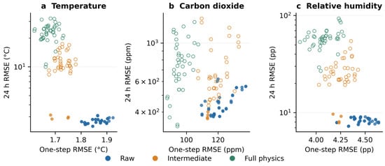
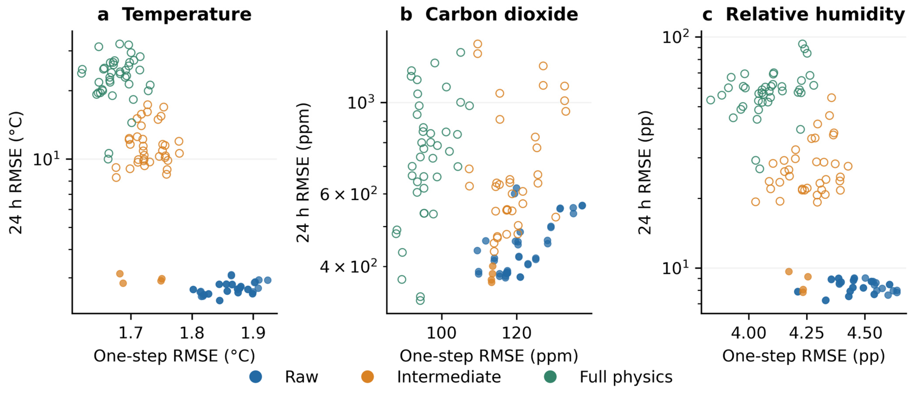
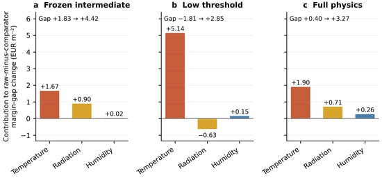
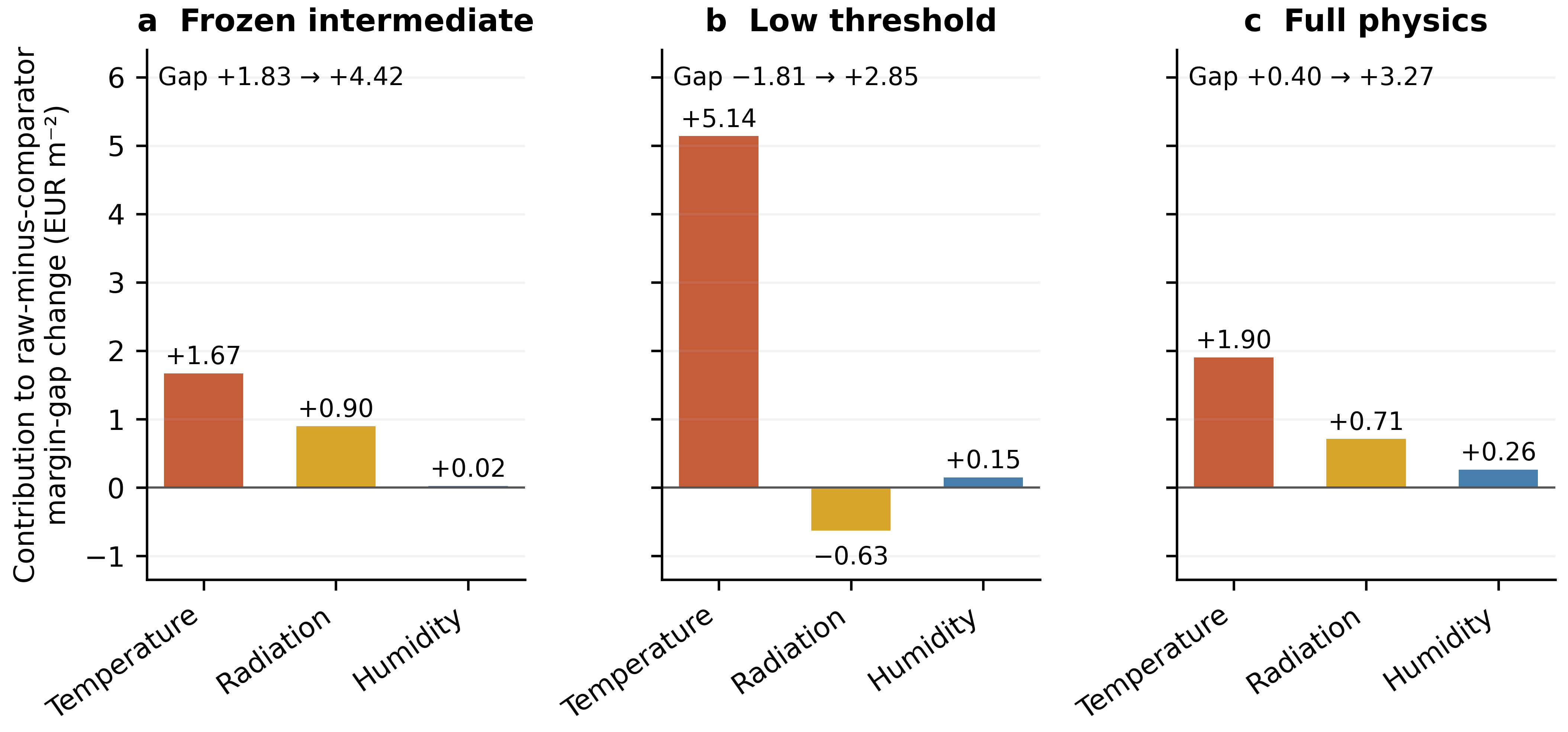
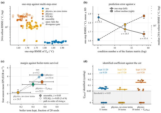
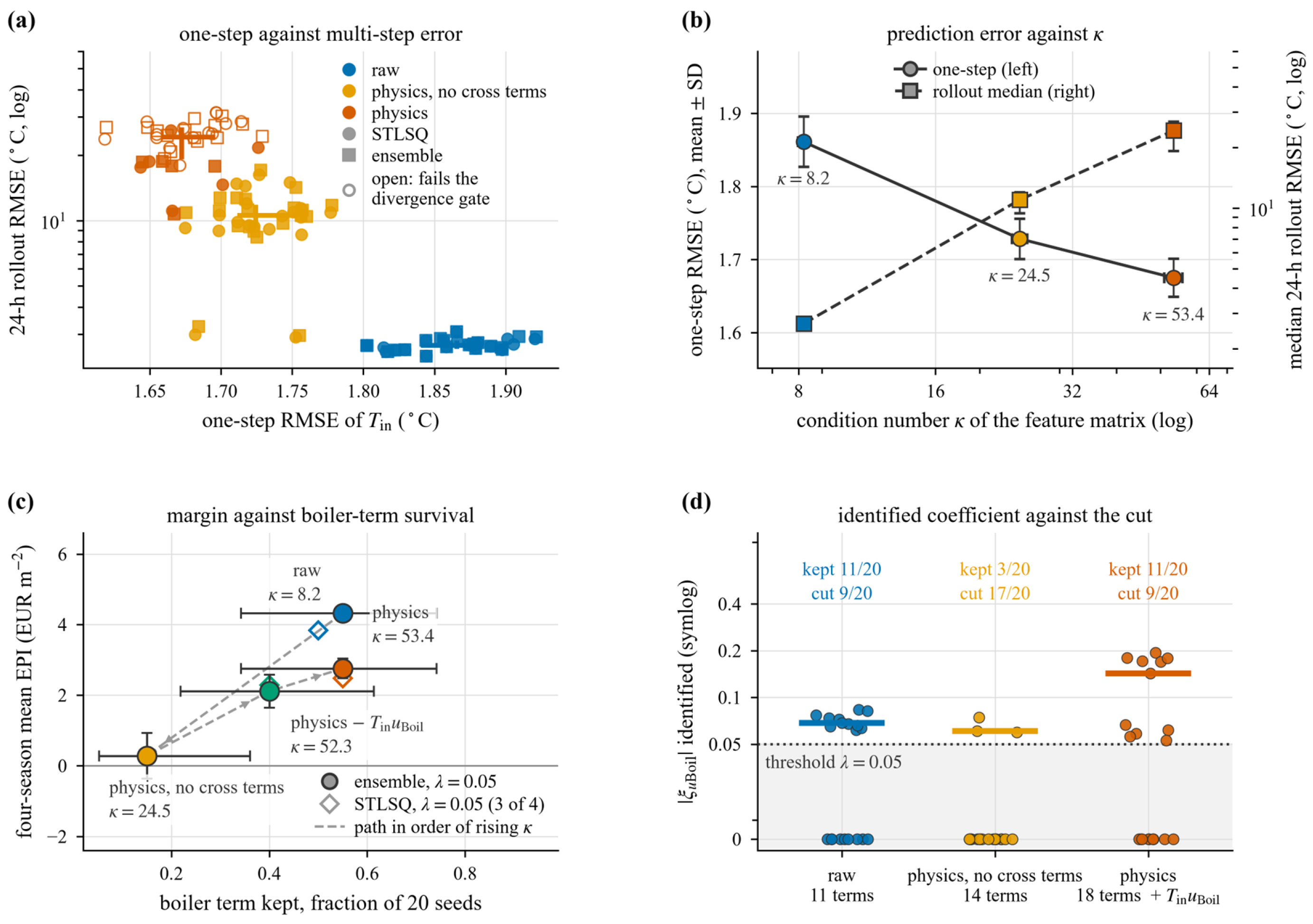
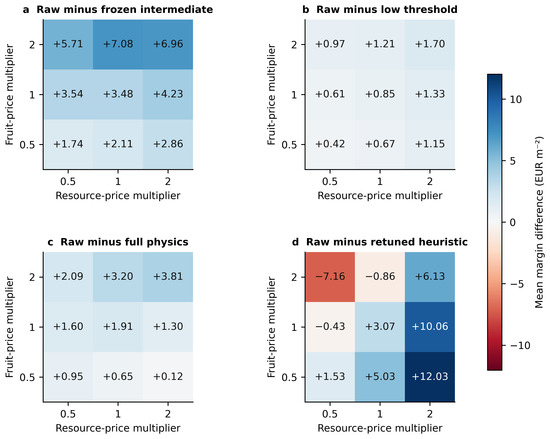
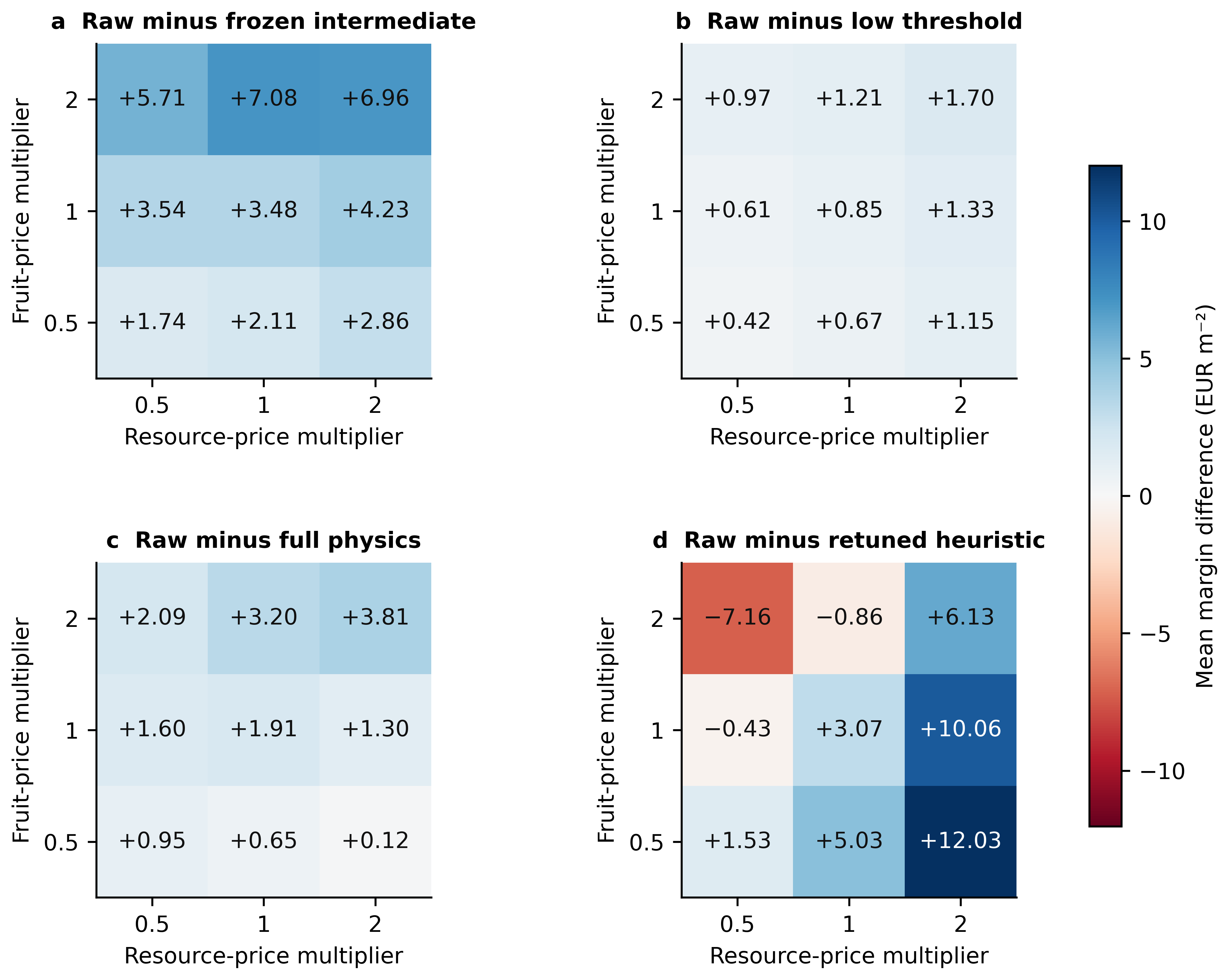

Disclaimer/Publisher’s Note: The statements, opinions and data contained in all publications are solely those of the individual author(s) and contributor(s) and not of MDPI and/or the editor(s). MDPI and/or the editor(s) disclaim responsibility for any injury to people or property resulting from any ideas, methods, instructions or products referred to in the content. |
© 2026 by the authors. Licensee MDPI, Basel, Switzerland. This article is an open access article distributed under the terms and conditions of the Creative Commons Attribution (CC BY) license.