Power-Circle Vulnerability Assessment and Two-Stage IPSO-Based Multi-STATCOM Allocation for Fine Voltage Regulation in Distribution Networks

Abstract

A two-stage improved particle swarm optimization (IPSO) framework is proposed for multi-STATCOM siting and sizing in radial distribution networks, together with a power-circle external-tangency margin for independent electrical-vulnerability assessment. The power-circle margin is formulated from branch active- and reactive-power circle relationships, aggregated by the arithmetic mean of incident-branch margins to avoid topological-degree bias, and cross-checked against Q–V continuation-power-flow results and load-level sensitivity. STATCOM planning minimizes the annual cost of active-power losses, annualized device investment, and operation and maintenance under hard voltage constraints. In the first optimization stage, two installation locations and coarse capacities are searched jointly; the second stage fixes the selected locations and continuously refines the capacities. On the IEEE 33-bus system, the power-circle and Q–V rankings show a Spearman correlation of 0.8644 and 90% Top-10 overlap. Deterministic enumeration identifies Bus 7 with 3.6689 Mvar as the best single-STATCOM solution, whereas the optimal dual configuration is 0.5583 Mvar at Bus 16 and 1.1571 Mvar at Bus 30. The dual solution reduces annual cost by 38.86% relative to the optimal single-device solution and reduces active-power loss to 0.1402 MW while satisfying all normal-operation voltage limits. Across 30 independent runs on the dual-device problem, the proposed IPSO attains the highest location-pair and global-solution success rates (33.33%) and the lowest mean objective value among six compared algorithms. Under restored N − 1 contingencies, the normal-operation economic optimum improves post-contingency voltage performance but is capacity-limited; with the locations fixed, a total rating of 6.5693 Mvar is required to satisfy all 31 restorable contingencies, revealing the trade-off between normal-operation economy and post-contingency voltage compliance.

1. Introduction

Increasing penetration of distributed energy resources and power-electronic interfaces has made reactive-power management in distribution networks increasingly important. Insufficient local reactive support can aggravate voltage drops and network losses, whereas excessive compensation increases investment and may distort the voltage profile. Distribution static synchronous compensators (D-STATCOMs/STATCOMs) provide continuously controllable reactive power and fast steady-state voltage support, but their effectiveness depends strongly on where they are installed and how much capacity is deployed.

Existing studies have addressed D-STATCOM allocation using stochastic, metaheuristic, mixed-integer, and hybrid discrete–continuous optimization approaches [1,2,3,4,5,6,7,8,9]. Coordinated Volt/Var and PV-STATCOM operation have also been investigated for distribution-network voltage regulation and loss reduction [10,11,12]. These methods demonstrate that siting and sizing are inherently coupled: the same reactive capacity can have substantially different system-wide effects at different buses, while multi-device planning further expands the mixed discrete–continuous search space.

Electrical-weakness indicators provide a complementary physical view of the allocation problem. Voltage-stability indices, Q–V/P–V analysis, and power-circle formulations can identify buses or regions that are closer to a voltage-solvability boundary [13,14,15]. However, an electrically weak bus is not necessarily the economically optimal compensation location because the latter also depends on network-wide voltage constraints, power-loss redistribution, and device cost. Consequently, weakness assessment and siting optimization should be comparatively assessed separately rather than assuming that the weakest bus must be the optimal installation bus.

A second limitation in many optimization studies is the lack of an independent deterministic benchmark and repeated-run statistics. When the search space is small, a metaheuristic can appear effective even when a simpler method can recover the same optimum. Conversely, multi-device planning creates a substantially larger combinatorial problem in which location recovery rate, robustness, and convergence behavior become more informative than a single best objective value. In addition, normal-operation economic planning does not automatically guarantee post-contingency voltage compliance, so contingency performance should be evaluated explicitly. A comparison of representative reactive-power compensation and STATCOM planning approaches is summarized in Table 1.

Table 1. Comparison of representative reactive-power compensation and STATCOM planning approaches.

Reference	Device/Method	Test System	Siting/Sizing Method	Voltage-Stability/Weakness Validation	Multiple Devices	N − 1 Analysis	Deterministic Benchmark
Tahir et al. [16]	Shunt capacitor	Distribution systems	Analytical, heuristic, and hybrid capacitor-placement methods	Not specifically reported	Discussed in reviewed literature	No	No
Alemu and Meseret [17]	SVC	IEEE 33-bus	Optimal capacitor placement-based SVC location and rating	Voltage-profile assessment	Yes	No	No
Yenealem [8]	MG + D-STATCOM	IEEE 30-bus RDS	LSF/VSI for location + PSO for sizing	VSI used for MG placement	Yes	No	No
Suárez Patiño et al. [7]	D-STATCOM	33-, 69-, 136-bus systems	MILP-based joint placement, sizing, and operation	Voltage constraints/multi-period assessment	Yes	No	Optimization-model optimum
Xiong et al. [11]	PV inverter Volt/VAR	IEEE 33- and 123-bus	SAC-based coordinated Volt/VAR control	Voltage-violation performance	Multiple inverters	No	No
Sharma et al. [14]	Power-circle assessment	Active distribution network	Power-circle/continuation-OPF formulation	Power-circle-based flexibility assessment	Not a device-planning study	No	No
This work	Dual STATCOM + Power-Circle + IPSO	IEEE 33-bus	Two-stage mixed discrete–continuous IPSO; all-bus/all-pair deterministic benchmark	Power-Circle ranking compared with Q–V	Yes	Yes	Yes

Table 1. Comparison of representative reactive-power compensation and STATCOM planning approaches.

Reference	Device/Method	Test System	Siting/Sizing Method	Voltage-Stability/Weakness Validation	Multiple Devices	N − 1 Analysis	Deterministic Benchmark
Tahir et al. [16]	Shunt capacitor	Distribution systems	Analytical, heuristic, and hybrid capacitor-placement methods	Not specifically reported	Discussed in reviewed literature	No	No
Alemu and Meseret [17]	SVC	IEEE 33-bus	Optimal capacitor placement-based SVC location and rating	Voltage-profile assessment	Yes	No	No
Yenealem [8]	MG + D-STATCOM	IEEE 30-bus RDS	LSF/VSI for location + PSO for sizing	VSI used for MG placement	Yes	No	No
Suárez Patiño et al. [7]	D-STATCOM	33-, 69-, 136-bus systems	MILP-based joint placement, sizing, and operation	Voltage constraints/multi-period assessment	Yes	No	Optimization-model optimum
Xiong et al. [11]	PV inverter Volt/VAR	IEEE 33- and 123-bus	SAC-based coordinated Volt/VAR control	Voltage-violation performance	Multiple inverters	No	No
Sharma et al. [14]	Power-circle assessment	Active distribution network	Power-circle/continuation-OPF formulation	Power-circle-based flexibility assessment	Not a device-planning study	No	No
This work	Dual STATCOM + Power-Circle + IPSO	IEEE 33-bus	Two-stage mixed discrete–continuous IPSO; all-bus/all-pair deterministic benchmark	Power-Circle ranking compared with Q–V	Yes	Yes	Yes

The main contributions of this study can be summarized as follows:

(1)

A power-circle external-tangency margin is formulated as an electrical-vulnerability indicator rather than a direct siting rule. Branch margins are directionally evaluated and averaged at the bus level to reduce topological-degree bias. Its ranking consistency is quantified against Q–V continuation-power-flow results and across multiple loading levels.

(2)

A two-stage IPSO framework is developed for a mixed discrete–continuous multi-STATCOM problem under hard voltage constraints. The first stage searches two locations and coarse capacities over the full candidate set, while the second stage continuously refines the capacities at the selected locations. Deterministic enumeration is used as an independent benchmark, and the proposed IPSO is compared with SPSO, LDW-PSO, TVAC-PSO, GA, and WOA over 30 independent runs.

(3)

Single- and dual-STATCOM configurations are compared on the IEEE 33-bus radial distribution system. The normal-operation economic optimum is further evaluated under restored N − 1 line contingencies, and a fixed-location capacity-reinforcement analysis quantifies the additional installed STATCOM capacity required to achieve full post-contingency voltage compliance.

2. Reactive Power Compensation Optimization Model for Distribution Networks

The planning model represents each STATCOM as a controllable shunt reactive-power source connected to a selected bus. Detailed converter switching and inner-loop dynamics are outside the scope of this steady-state planning study. For a STATCOM installed at bus i, positive QCi denotes capacitive reactive-power injection and is modeled by reducing the net reactive demand at that bus. The model simultaneously accounts for network loss cost and annualized STATCOM cost while enforcing AC power-flow and voltage constraints.

2.1. Economic Objective Function

The annual economic objective is defined as

$$\min F_{\mathit{econ}}=F_1+F_2+F_3$$

(1)

where F₁ is the annual active-power-loss cost, F₂ is the annualized STATCOM investment, and F₃ is the annual operation-and-maintenance cost.

$$F_1=P_{\mathrm{loss}}\times {10}^3{K}_{e}T$$

(2)

$$F_2=\left({\displaystyle \sum _{j=1}^{N_C}{Q}_{C,j}^{\mathrm{rated}}}\right)\times {10}^3{C}_q\cdot \mathrm{CRF}$$

(3)

$$\mathrm{CRF}={\displaystyle \frac{r{(1+r)}^n}{{(1+r)}^n-1}}$$

(4)

$$F_3=k_{\mathit{OM}}{F}_2$$

(5)

where P_loss denotes the total active-power loss of the distribution network, in MW; K_e is the electricity price, in USD/kWh; and T is the equivalent annual operating time, in h/year. N_C is the number of installed STATCOMs and $Q_{C,j}^{\mathrm{rated}}$ denotes the rated reactive-power capacity of the j-th STATCOM, in Mvar. C_q is the unit-capacity investment cost of the STATCOM, in USD/kvar. The capital recovery factor (CRF) converts the initial investment into an equivalent annual cost, where r is the annual discount rate and n is the service life of the STATCOM, in years. k_OM denotes the annual operation-and-maintenance cost ratio.

All economic results reported in the case study are calculated using the same parameter set listed in Table 2 and Equations (1)–(5). The adopted STATCOM investment model is proportional to the rated reactive-power capacity and does not include a fixed installation cost per device. Therefore, the reported economic comparison between the single- and dual-STATCOM configurations is conditional on this cost assumption.

Table 2. IEEE 33-bus system, economic, and optimization parameters.

Parameter	Value	Unit
Test system	MATPOWER case33bw	–
Base MVA	10	MVA
Base voltage	12.66	kV
Total active load	3.715	MW
Total reactive load	2.3	Mvar
Voltage lower bound	0.95	p.u.
Voltage upper bound	1.05	p.u.
Energy price, Ke	0.139	USD/kWh
Equivalent annual operating hours, T	2190	h/year
STATCOM unit capacity cost, Cq	50	USD/kvar
Discount rate, r	0.1	–
Lifetime, n	30	year
Capital recovery factor, CRF	0.106079	1/year
O&M ratio	0.05	–
Single-STATCOM Q bound	0–10	Mvar
Dual-STATCOM Q bound per device	0–10	Mvar
Power-flow solver	MATPOWER Newton–Raphson AC power flow	–
Power-flow tolerance	1.0 × 10−10	p.u.
Constraint handling	Hard voltage constraints + Deb feasibility rules	–

2.2. AC Power-Flow and Operating Constraints

For each evaluated configuration, the AC nodal power-balance equations are satisfied:

$$P_{G,i}-P_{D,i}=V_i{\displaystyle \sum _{j=1}^{N_B}{V}_j}[G_{\mathit{ij}}\cos ({\theta }_i-{\theta }_j)+B_{\mathit{ij}}\sin ({\theta }_i-{\theta }_j)]$$

(6)

$$Q_{G,i}+Q_{C,i}-Q_{D,i}=V_i{\displaystyle \sum _{j=1}^{N_B}{V}_j}[G_{\mathit{ij}}\sin ({\theta }_i-{\theta }_j)-B_{\mathit{ij}}\cos ({\theta }_i-{\theta }_j)]$$

(7)

The principal inequality constraints are:

$$0.95\le V_i\le 1.05$$

(8)

$$0\le Q_{C,j}\le Q_{C,j}^{\max }$$

(9)

where P_G,i and Q_G,i are the active- and reactive-power outputs of the generator connected to bus i, respectively; P_D,i and Q_D,i are the active- and reactive-power demands at bus i; and Q_C,i denotes the reactive-power injection provided by a STATCOM at bus i. For buses without a STATCOM, Q_C,i = 0. V_i and V_j denote the voltage magnitudes of buses i and j, while θ_i and θ_j are the corresponding voltage phase angles. G_ij and B_ij are the conductance and susceptance elements of the network bus-admittance matrix, respectively, and N_B is the total number of buses in the system.

The bus-voltage magnitude is constrained within the allowable operating range of 0.95–1.05 p.u. For the j-th installed STATCOM, Q_C,j denotes its reactive-power output and $Q_{C,j}^{\max }$ is its maximum available reactive-power capacity.

To quantitatively evaluate the overall bus-voltage deviation before and after reactive-power compensation, the aggregate voltage-deviation index D_U is defined as

$$D_U={\displaystyle \sum _{i=1}^{N_B}\left|V_i-1\right|}$$

(10)

A smaller D_U indicates that the overall bus-voltage profile is closer to the nominal voltage level. The index is used only for performance evaluation and comparison and is not included in the economic objective function.

2.3. Single- and Dual-STATCOM Planning Scenarios

Both single- and dual-device configurations are evaluated. All PQ buses (Buses 2–33) are retained as potential locations, and no Power-Circle-based hard screening is applied. The single-device deterministic benchmark therefore considers all 32 locations. For the dual-device case, all C(32,2) = 496 unordered location pairs are examined in the deterministic benchmark. This separation is important because the bus with the smallest electrical weakness margin need not be the location that minimizes the system-wide annual cost under voltage constraints.

3. Power-Circle-Based Voltage-Solvability Assessment

The power-circle formulation is used in this study as an electrical-vulnerability assessment tool and as a post-compensation evaluation metric. It is not used to remove candidate buses or bias the optimization population. This distinction allows the electrical-weakness assessment and the economic siting result to be validated independently.

3.1. Power-Circle Formulation and Branch External-Tangency Margin

Consider an arbitrary AC branch in the distribution network. Let the sending and receiving buses be denoted by F and S, respectively. The branch impedance is Z_SF = R_SF + jX_SF, and the corresponding sending- and receiving-end voltages, branch current, and active/reactive powers are defined as shown in Figure 1.

Figure 1. AC Branch of the Power System.

The branch voltage relationship can be expressed as:

$${\dot{U}}_S={\dot{U}}_F-{\dot{I}}_{\mathit{FS}}(R_{\mathit{FS}}+j{X}_{\mathit{FS}})$$

(11)

Taking the sending-end voltage ${\dot{U}}_F=U_F\angle 0$ as the reference phasor and decomposing the receiving-end voltage ${\dot{U}}_S$ and branch current ${\dot{I}}_{\mathit{FS}}$ into their real and imaginary components yields:

$$\left\{\begin{array}{l}\begin{array}{l}{U}_{\mathit{Sx}}=U_F-(I_{\mathit{FSx}}{R}_{\mathit{FS}}-I_{\mathit{FSy}}{X}_{\mathit{FS}})\\ U_{\mathit{Sy}}=-(I_{\mathit{FSx}}{X}_{\mathit{FS}}+I_{\mathit{FSy}}{R}_{\mathit{FS}})\end{array}\hfill \end{array}\right.$$

(12)

where U_Sx and U_Sy are the real and imaginary components of the receiving-end voltage ${\dot{U}}_S$, respectively, and I_FSx and I_FSy are the real and imaginary components of the branch current ${\dot{I}}_{\mathit{FS}}$, respectively.

Under the adopted F → S branch-current direction, P_SF and Q_SF are defined as positive when active and reactive power are delivered by the branch to the receiving bus S. The receiving-end complex power is therefore:

$$P_{\mathit{SF}}+j{Q}_{\mathit{SF}}={\dot{U}}_S{\dot{I}}_{\mathit{FS}}^{*}$$

(13)

Expanding Equation (13) gives

$$\left\{\begin{array}{l}\begin{array}{l}{P}_{\mathit{SF}}=U_{\mathit{Sx}}{I}_{\mathit{FSx}}+U_{\mathit{Sy}}{I}_{\mathit{FSy}}\\ Q_{\mathit{SF}}=U_{\mathit{Sy}}{I}_{\mathit{FSx}}-U_{\mathit{Sx}}{I}_{\mathit{FSy}}\end{array}\hfill \end{array}\right.$$

(14)

Eliminating the current components from the preceding equations gives the relationship between the receiving-end power and receiving-end voltage components:

$$\left\{\begin{array}{l}{P}_{\mathit{SF}}=-g_{\mathit{FS}}{U}_{\mathit{Sx}}^2+g_{\mathit{FS}}{U}_F{U}_{\mathit{Sx}}-g_{\mathit{FS}}{U}_{\mathit{Sy}}^2+b_{\mathit{FS}}{U}_F{U}_{\mathit{Sy}}\hfill \\ Q_{\mathit{SF}}=b_{\mathit{FS}}{U}_{\mathit{Sx}}^2-b_{\mathit{FS}}{U}_F{U}_{\mathit{Sx}}+b_{\mathit{FS}}{U}_{\mathit{Sy}}^2+g_{\mathit{FS}}{U}_F{U}_{\mathit{Sy}}\hfill \end{array}\right.$$

(15)

The branch admittance is:

$$Y_{\mathit{FS}}={\displaystyle \frac{1}{R_{\mathit{FS}}+j{X}_{\mathit{FS}}}}=g_{\mathit{FS}}+j{b}_{\mathit{FS}}$$

(16)

For a conventional inductive branch, the series susceptance satisfies b_FS < 0. To avoid sign ambiguity in the subsequent power-circle derivation, we define g = g_FS > 0 and b = −b_FS > 0. Thus, the branch series admittance can equivalently be written as Y_FS = g − jb. Substituting g_FS = g and b_FS = −b into Equation (15) and completing the square with respect to the receiving-end voltage components, the active and reactive-power equations can be expressed in the standard circle forms as follows.

$${\left(U_{\mathit{Sx}}-{\displaystyle \frac{U_F}{2}}\right)}^2+{\left(U_{\mathit{Sy}}+{\displaystyle \frac{b{U}_F}{2g}}\right)}^2={\displaystyle \frac{U_F^2}{4}}+{\displaystyle \frac{b^2{U}_F^2}{4g^2}}-{\displaystyle \frac{P_{\mathit{SF}}}{g}}$$

(17)

$${\left(U_{\mathit{Sx}}-{\displaystyle \frac{U_F}{2}}\right)}^2+{\left(U_{\mathit{Sy}}-{\displaystyle \frac{g{U}_F}{2b}}\right)}^2={\displaystyle \frac{U_F^2}{4}}+{\displaystyle \frac{g^2{U}_F^2}{4b^2}}-{\displaystyle \frac{Q_{\mathit{SF}}}{b}}$$

(18)

The radii of the active-power circle and reactive-power circle are given by:

$$r_P=\sqrt{{\displaystyle \frac{U_F^2}{4}}+{\displaystyle \frac{b^2{U}_F^2}{4g^2}}-{\displaystyle \frac{P_{\mathit{SF}}}{g}}}$$

(19)

$$r_Q=\sqrt{{\displaystyle \frac{U_F^2}{4}}+{\displaystyle \frac{g^2{U}_F^2}{4b^2}}-{\displaystyle \frac{Q_{\mathit{SF}}}{b}}}$$

(20)

The distance D between the centers of the two circles can therefore be obtained as:

$$D={\displaystyle \frac{g^2+b^2}{2\mathit{gb}}}{U}_F$$

(21)

For the active- and reactive-power circles to have a common voltage solution, the following geometric intersection condition should be satisfied:

$$\left\{\begin{array}{l}{r}_P\ge 0\hfill \\ r_Q\ge 0\hfill \\ \left|r_P-r_Q\right|\le D\le r_P+r_Q\hfill \end{array}\right.$$

(22)

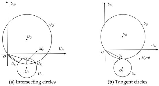
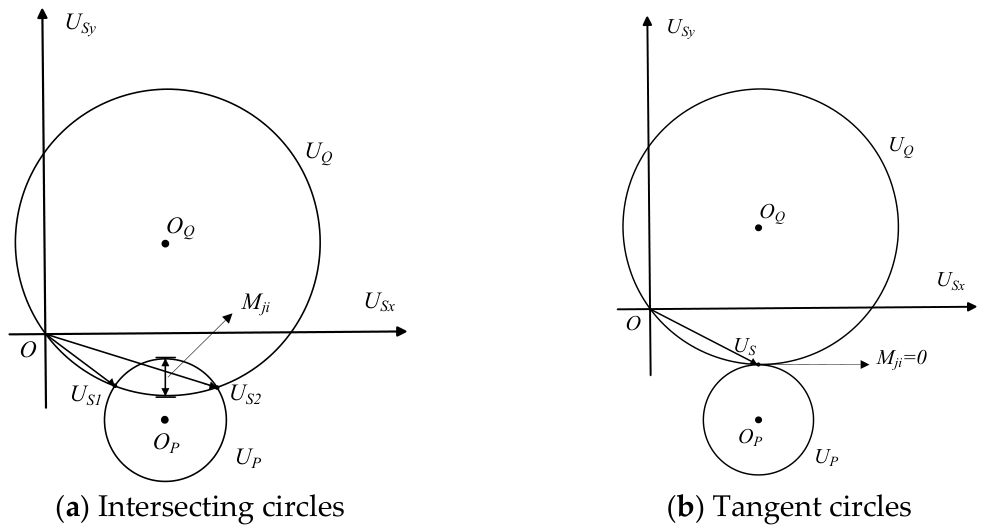
The geometric relationship between the active- and reactive-power circles under the intersecting and external-tangency conditions is illustrated in Figure 2.

Figure 2. Geometric relationship between the active- and reactive-power circles: (a) intersecting state; (b) external-tangency state.

After the complete circle-intersection condition in Equation (22) is satisfied, the directional branch power-circle margin with respect to the external-tangency boundary is defined as:

$$M_{\mathit{ji}}=r_P+r_Q-D$$

(23)

Equation (23) specifically quantifies the geometric margin to the external-tangency boundary D = r_P + r_Q, i.e., the slack of the upper intersection condition D ≤ r_P + r_Q. It does not represent the distance to the internal-tangency boundary D = |r_P − r_Q|. Therefore, the complete intersection condition in Equation (22) is checked independently before M_ji is interpreted.

A larger positive M_ji indicates a greater geometric separation from the external-tangency boundary, whereas M_ji = 0 corresponds to external tangency. A negative value indicates violation of the external-intersection condition. The quantity M_ji is a geometric power-circle external-tangency margin and should not be interpreted as a remaining reactive-power reserve in Mvar or as a direct measure of whole-system voltage stability.

The mathematical consistency of Equations (13)–(23) is further verified using independently obtained AC power-flow operating points in Section 5.2.

3.2. Bus Aggregation and Special Branch Handling

Because buses can have different numbers of incident branches, directly summing branch margins introduces a topological-degree bias. The bus-level indicator is therefore defined as the arithmetic mean of all incident directional branch margins:

$$M_i={\displaystyle \frac{1}{N_i}}{\displaystyle \sum _{j\in {\mathsf{\Omega }}_i}\left(r_{P,\mathit{ij}}+r_{Q,\mathit{ij}}-D_{\mathit{ij}}\right)}$$

(24)

where N_i denotes the number of branches incident on bus i, and Ω_i is the corresponding incident-branch set. A smaller M_i indicates that bus i and its neighboring branches are, on average, closer to the power-circle external-tangency boundary, and therefore represent a relatively vulnerable region of the network.

For a zero-resistance branch, R_SF = 0, and the real part of the series admittance consequently satisfies g = 0. In this case, the general power-circle expressions containing 1/g become singular. Therefore, such branches are treated separately rather than approximating g by an artificially small positive value. Under the sign convention b = −b_FS > 0, the active-power-circle relationship degenerates into a straight line.

$$U_{\mathit{Sy}}=-{\displaystyle \frac{P_{\mathit{SF}}}{b{U}_F}}$$

(25)

whereas the reactive-power relationship remains circular and can be expressed as

$${\left(U_{\mathit{Sx}}-{\displaystyle \frac{U_F}{2}}\right)}^2+{U_{\mathit{Sy}}}^2={\displaystyle \frac{U_F^2}{4}}-{\displaystyle \frac{Q_{\mathit{SF}}}{b}}$$

(26)

Accordingly, the radius of the reactive-power circle is

$$r_Q=\sqrt{{\displaystyle \frac{U_F^2}{4}}-{\displaystyle \frac{Q_{\mathit{SF}}}{b}}}$$

(27)

and the perpendicular distance from the center of the reactive-power circle to the active-power line is

$$d=\left|{\displaystyle \frac{P_{\mathit{SF}}}{b{U}_F}}\right|$$

(28)

A common voltage solution exists when d ≤ r_Q, while d = r_Q corresponds to the tangent condition. Therefore, for a zero-resistance branch, the corresponding power-circle line–circle tangency margin is defined as

$$M_{\mathit{ij}}^{(g=0)}=r_Q-d$$

(29)

A positive value indicates that the active-power line intersects the reactive-power circle, zero represents the critical tangent condition, and a negative value indicates that no common voltage solution exists under the considered operating condition. This special treatment avoids the singularity caused by g = 0 and allows zero-resistance branches to be consistently included in the bus-level margin calculation.

3.3. Comparative Assessment of the Power-Circle Margin Using Q–V Analysis

The power-circle margin is assessed from two complementary perspectives. First, the system loading level is scaled to 0.8, 1.0, and 1.2 times the base load, and the consistency of the bus-vulnerability ranking is evaluated using the Spearman rank-correlation coefficient and Top-(k) overlap. Second, node-specific Q–V curves are obtained using continuation power flow and are used as an independent comparative benchmark for electrical vulnerability.

For each non-slack bus i, the Q–V nose-point reactive-demand margin is defined as $Q_{D,i}^{\mathrm{nose}}-Q_{D,i}^0$, where $Q_{D,i}^0$ is the reactive-power demand at the base operating point, and $Q_{D,i}^{\mathrm{nose}}$ is the corresponding reactive-power demand at the continuation-power-flow nose point. A smaller $\Delta Q_i^{\mathrm{nose}}$ indicates that less additional reactive demand is required to reach the Q–V nose point and therefore represents greater electrical vulnerability.

For the power-circle indicator, a smaller bus-level margin M_i likewise represents greater vulnerability. Therefore, all 32 non-slack buses are ranked in ascending order for both indicators, with Rank 1 corresponding to the smallest margin. The Spearman coefficient is calculated between the complete power-circle and Q–V ranking vectors. The Top-(k) overlap is defined as the percentage of buses that are simultaneously included in the (k) most vulnerable buses identified by the two indicators.

The Q–V comparison is intended to evaluate the consistency of the identified vulnerable regions rather than to establish numerical equivalence between the two margins. The power-circle margin is a local geometric external-tangency indicator, whereas the Q–V nose-point margin is a continuation-based reactive-demand margin. In addition, the Q–V calculation retains a common bus-type formulation without reactive-power-limit switching; therefore, the resulting Q–V margin is not interpreted as an operational reactive-power reserve.

4. Two-Stage IPSO for Multi-STATCOM Siting and Sizing

The final optimization problem contains discrete installation locations and continuous capacities. For the dual-device case, the location space alone contains 496 unordered bus pairs. A two-stage solution is therefore adopted so that the first stage performs mixed location/coarse-capacity exploration, and the second stage continuously refines capacities at the selected locations.

4.1. Stage 1: Mixed Siting and Coarse Sizing

Each Stage-1 particle is represented by X = [x₁,x₂,Q₁,Q₂]. The latent location variables x₁ and x₂ are bounded to [2, 33], rounded to integer bus indices, repaired if both map to the same bus, and finally placed in canonical ascending order. The corresponding Q₁ and Q₂ values are bounded to [0, 10] Mvar and decoded to a 0.05-Mvar grid. All 32 candidate buses are initialized uniformly; no Power-Circle, Q–V, or sensitivity-based bias is introduced.

4.2. Stage 2: Continuous Capacity Refinement

After Stage 1 identifies a location pair, the two buses are fixed, and Q₁ and Q₂ are optimized continuously over [0, 10] Mvar. AC power flow is embedded in every fitness evaluation, and the same economic objective and Deb feasibility rules are used in both stages.

4.3. IPSO Updating Strategy

The standard PSO formulation follows Kennedy and Eberhart [18]. The inertia-weight strategy and time-varying acceleration coefficients are implemented following the established PSO developments in [19,20], while related convergence and algorithm-development analyses are provided in [21,22].

The standard particle velocity and position equations are

$$v_{i,d}^{k+1}={\omega }^k{v}_{i,d}^k+c_1^k{r}_1(p_{i,d}^{\mathrm{best}}-x_{i,d}^k)+c_2^k{r}_2(g_d^{\mathrm{best}}-x_{i,d}^k)$$

(30)

$$x_{i,d}^{k+1}=x_{i,d}^k+v_{i,d}^{k+1}$$

(31)

The proposed IPSO uses a decreasing inertia weight and time-varying learning factors:

$${\omega }^k={\omega }_{\max }-{\displaystyle \frac{{\omega }_{\max }-{\omega }_{\min }}{K_{\max }}}k$$

(32)

$$c_1^k=c_{1,\max }-{\displaystyle \frac{c_{1,\max }-c_{1,\min }}{K_{\max }}}k$$

(33)

$$c_2^k=c_{2,\min }+{\displaystyle \frac{c_{2,\max }-c_{2,\min }}{K_{\max }}}k$$

(34)

where i and d denote the particle index and search dimension, respectively; k is the current iteration and K_max is the maximum number of iterations; $x_{i,d}^k$ and $v_{i,d}^{k+1}$ are the position and velocity of particle i in dimension d; $p_{i,d}^{\mathrm{best}}$ and $g_d^{\mathrm{best}}$ denote the personal and global best positions, respectively; and r₁ and r₂ are independent random numbers uniformly distributed in [0, 1].

The adopted ranges are ω: 0.9 → 0.4, c₁: 2.5 → 1.0, and c₂: 1.0 → 2.5. The method is evaluated against a fixed-parameter SPSO, a linearly decreasing-inertia-weight PSO (LDW-PSO), a TVAC-only PSO, GA, and WOA under the same population size and iteration budget.

4.4. Deterministic Benchmark and Statistical Evaluation

To avoid evaluating the metaheuristics only against one another, deterministic baselines are established independently. For the single-device case, every candidate bus is evaluated and its continuous capacity is refined at high precision. For the dual-device case, all 496 unordered location pairs are scanned and subsequently refined by deterministic continuous optimization. Algorithm performance is then assessed over 30 independent runs using final objective statistics, optimal-location-pair recovery rate, global-solution success rate, convergence history, power-flow evaluation count, and runtime.

All simulations were implemented in MATLAB R2024a using MATPOWER 8.1 on a 64-bit Windows workstation equipped with an Intel Core i5-13600KF processor and 32 GB of RAM. A six-worker local process pool was used for the independent runs. For each algorithm, 30 independent runs were performed using fixed, non-overlapping MATLAB Mersenne Twister random seeds, which were retained in the simulation records to permit exact reruns. All algorithms used a population size of 30 and 50 iterations in each optimization stage, corresponding to 3000 objective-function and AC power-flow evaluations per complete run. The same IEEE 33-bus data, Newton–Raphson power-flow solver, 10⁻¹⁰ convergence tolerance, 0.95–1.05 p.u. voltage limits, economic parameters, STATCOM capacity bounds, Deb feasibility rules, and iteration budget were used throughout. A run was classified as globally successful only when the optimal location pair (Buses 16 and 30) was recovered, the capacity deviations from the deterministic optimum did not exceed 0.01 Mvar, the annual-cost deviation did not exceed 0.10%, and the final AC power flow converged with all voltage constraints satisfied within a 10⁻⁹ p.u. tolerance.

5. Case Study

5.1. IEEE 33-Bus Test System and Parameters

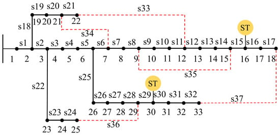
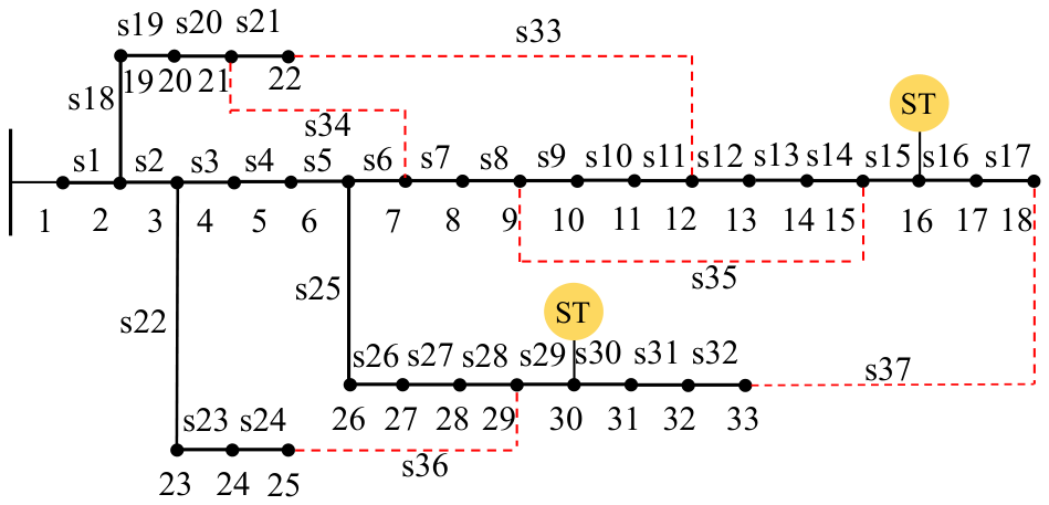
Simulations are carried out on the IEEE 33-bus radial distribution system implemented in MATPOWER case33bw, with a base power of 10 MVA. As shown in Figure 3, the system consists of 33 buses and 37 branches. Under normal operating conditions, switches S₁ − S₃₂ are closed to form the radial feeder structure, whereas tie switches S₃₃ − S₃₇, represented by red dashed lines, are normally open. Bus 1 serves as the slack bus, and Buses 2–33 are considered as candidate STATCOM installation locations. The total base load is 3.715 MW + j2.300 Mvar, and the permissible bus-voltage range is 0.95–1.05 p.u. The deterministic optimization results identify Buses 16 and 30 as the optimal locations for the dual-STATCOM configuration, as marked by “ST” in Figure 3.

Figure 3. IEEE 33-bus radial distribution system and the optimal dual-STATCOM locations. Black solid lines denote normally closed branches, red dashed lines denote normally open tie lines, numbers indicate bus indices, s1–s37 denote branch/switch indices, and the yellow “ST” markers indicate the optimal STATCOM locations at Buses 16 and 30.

The base case has an active-power loss of 0.202677 MW, a minimum voltage of 0.913090 p.u. at Bus 18, and 21 buses below the 0.95-p.u. lower limit. Hence, the uncompensated case is infeasible under the planning constraint and is used only as an operating reference.

5.2. Numerical Verification and Comparative Assessment of the Power-Circle Margin

5.2.1. Independent Branch-Level Verification

To independently verify the mathematical formulation, all 32 normally closed branches were checked using AC power-flow operating points obtained from MATPOWER. The receiving-end active and reactive powers were independently reconstructed from the complex bus voltages and branch impedances. The maximum absolute discrepancies were 2.35 × 10⁻¹⁴ p.u. for active power and 4.16 × 10⁻¹⁵ p.u. for reactive power. The maximum residuals of the active- and reactive-power circle equations were both 4.44 × 10⁻¹⁶. All 32 branches yielded nonnegative squared radii and satisfied the complete circle-intersection condition, while the center-distance expression agreed with direct geometric calculation within 2.22 × 10⁻¹⁶. These results confirm the adopted sign convention and the mathematical consistency of Equations (13)–(23). Representative verification results for five branches at different feeder locations are summarized in Table 3.

Table 3. Independent numerical verification of the power-circle formulation using representative IEEE 33-bus branch operating points.

Branch	From–To	${\mathit{P}}_{\mathit{SF}}^{\mathit{MP}}$ (p.u.)	${\mathit{P}}_{\mathit{SF}}^{\mathit{calc}}$ (p.u.)	|ΔP| (p.u.)	${\mathit{Q}}_{\mathit{SF}}^{\mathit{MP}}$ (p.u.)	${\mathit{Q}}_{\mathit{SF}}^{\mathit{calc}}$ (p.u.)	|ΔQ| (p.u.)	Active-Circle Residual	Reactive-Circle Residual
1	1–2	0.390543670	0.390543670	2.348 × 10−14	0.242890128	0.242890128	3.164 × 10−15	5.551 × 10−17	2.220 × 10−16
10	10–11	0.056021974	0.056021974	7.570 × 10−15	0.027424979	0.027424979	8.084 × 10−16	0	0
17	17–18	0.009000000	0.009000000	2.484 × 10−15	0.004000000	0.004000000	5.907 × 10−16	1.110 × 10−16	0
30	30–31	0.042022636	0.042022636	5.204 × 10−16	0.021026896	0.021026896	1.141 × 10−15	5.551 × 10−17	5.551 × 10−17
32	32–33	0.006000000	0.006000000	5.794 × 10−16	0.004000000	0.004000000	4.158 × 10−15	2.220 × 10−16	5.551 × 10−17

Note: $P_{\mathit{SF}}^{\mathit{MP}}$ and $Q_{\mathit{SF}}^{\mathit{MP}}$ denote the receiving-end branch powers obtained from the MATPOWER AC power-flow solution, whereas $P_{\mathit{SF}}^{\mathit{calc}}$ and $Q_{\mathit{SF}}^{\mathit{calc}}$ are independently reconstructed from the complex bus voltages and branch impedance according to the adopted F → S power-flow convention. The residuals denote the absolute differences between the left- and right-hand sides of the active- and reactive-power circle equations, respectively.

5.2.2. Load-Level and Q–V Comparative Assessment

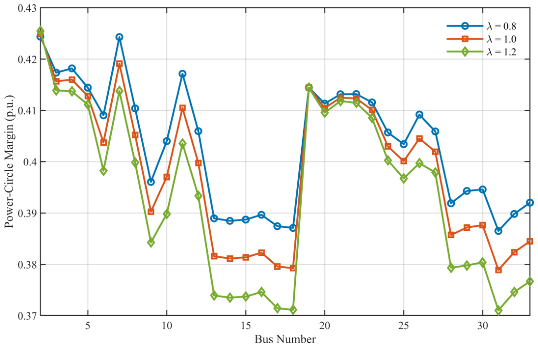
The bus-risk ordering remains highly consistent as loading changes. The Spearman correlations are 0.9919 for 0.8 versus 1.0 loading, 0.9923 for 1.0 versus 1.2, and 0.9780 for 0.8 versus 1.2, while the Top-5 vulnerable-bus sets overlap completely. This indicates that the indicator tracks the same weak network regions over the tested load range rather than being tied to a single operating snapshot. As shown in Figure 4, the bus-risk ordering remains highly consistent as loading changes.

Figure 4. Power-circle margins under three load levels.

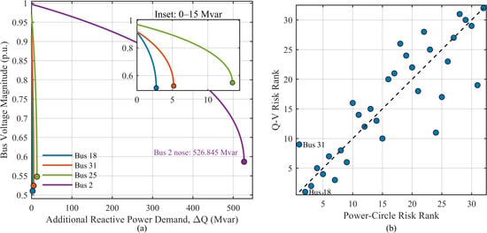
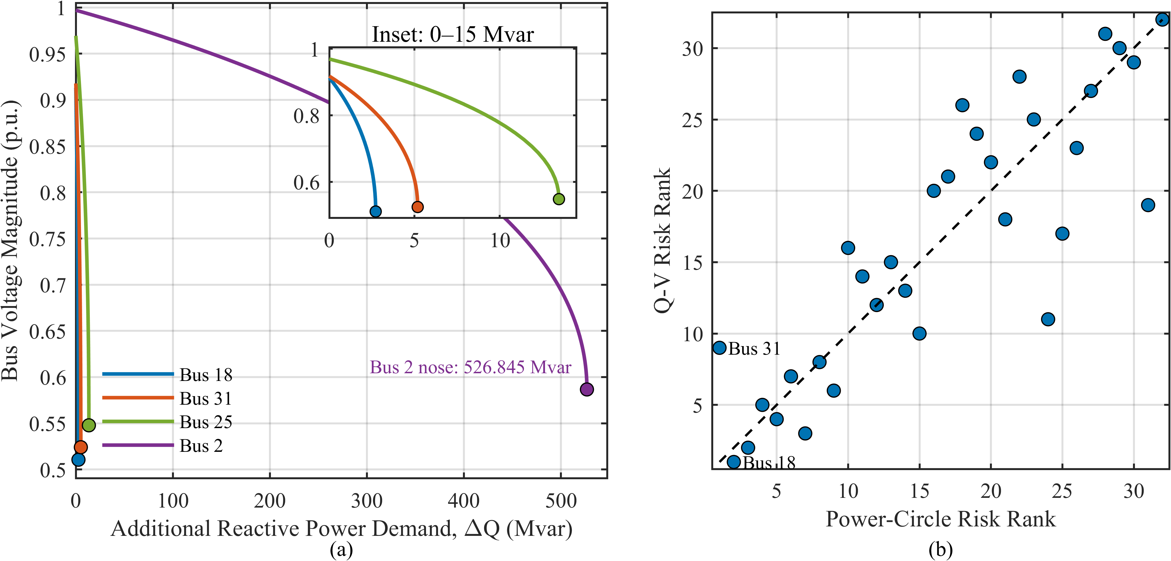
Figure 5 compares the Q–V nose-point margins with the power-circle vulnerability rankings.

Figure 5. Q–V comparative assessment of the power-circle margin: (a) representative Q–V curves with a local inset; (b) risk-rank comparison.

At the base loading level, the power-circle and Q–V rankings have a Spearman correlation of 0.8644. Their Top-3, Top-5, and Top-10 overlaps are 66.67%, 80%, and 90%, respectively. Bus 18 is the weakest bus according to Q–V nose-point margin (2.7222 Mvar), whereas Bus 31 has the smallest power-circle margin and ranks ninth in the Q–V ordering. The two indicators therefore identify largely the same weak region without being numerically identical, which is expected because one is a local geometric external-tangency indicator and the other is a Q–V nose-point reactive-demand margin. Therefore, the observed correlation supports ranking consistency between the two indicators but does not imply that the power-circle margin is numerically equivalent to the Q–V nose-point margin. The corresponding power-circle/Q–V ranking-consistency metrics are summarized in Table 4.

Table 4. Summary of power-circle/Q–V ranking-consistency results.

Category	Metric	Value
Load-level robustness	Spearman rank correlation, load 0.8 vs. 1.0	0.9919
Load-level robustness	Spearman rank correlation, load 1.0 vs. 1.2	0.9923
Load-level robustness	Spearman rank correlation, load 0.8 vs. 1.2	0.9780
Load-level robustness	Top-5 overlap, all load-level pairs	100.00%
Q–V comparison	Spearman rank correlation, PC vs. Q-V	0.8644
Q–V comparison	Top-3 overlap, PC vs. Q-V	66.67%
Q–V comparison	Top-5 overlap, PC vs. Q-V	80.00%
Q–V comparison	Top-10 overlap, PC vs. Q-V	90.00%
Q–V comparison	Q-V weakest bus	18
Q–V comparison	Power-Circle weakest bus	31

5.3. Deterministic Single- and Dual-STATCOM Results

A full deterministic benchmark is first established before comparing metaheuristics. For the single-device case, all 32 candidate buses are evaluated. Fourteen buses admit a feasible solution within the capacity bounds, and high-precision continuous refinement identifies Bus 7 with 3.6688619 Mvar and an annual cost of 85,454.08 USD/year as the global single-device optimum. The optimum lies on the lower-voltage constraint boundary.

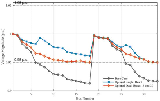
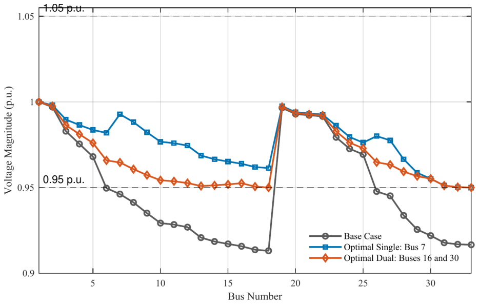
For the dual-device case, all 496 unordered location pairs are evaluated; 400 pairs admit feasible continuous solutions. The global optimum installs 0.5583256 Mvar at Bus 16 and 1.1571030 Mvar at Bus 30, for a total rating of 1.7154286 Mvar and an annual cost of 52,243.71 USD/year. Relative to the optimal single-device solution, the dual configuration reduces total installed capacity by 53.24% and annual cost by 38.86%. Its active-power loss is 0.140239 MW, below both the base case and the optimal single-device case. The corresponding bus-voltage profiles are shown in Figure 6, while the detailed quantitative comparison of the base case and the optimal single- and dual-STATCOM configurations is summarized in Table 5.

Figure 6. Bus-voltage profiles for the base case and the deterministic optimal single- and dual-STATCOM configurations.

Table 5. Deterministic comparison of the base, optimal single-STATCOM, and optimal dual-STATCOM configurations.

Configuration	Installation Bus (es)	STATCOM Capacity (Mvar)	Total Capacity (Mvar)	Annual Loss Cost F1 (USD/Year)	Annual STATCOM Cost F2 + F3 (USD/Year)	Total Feco (USD/Year)	ActivePower Loss (MW)	Voltage Deviation Index DU	Umin p.u.	Voltage Violations	Feasible
Base Case	–	–	–	61,696.94	–	Not applicable	0.2027	1.7009	0.9131	21	No
Optimal Single STATCOM	Bus 7	3.6689	3.6689	65,021.60	20,432.48	85,454.08	0.2136	0.7731	0.9500	0	Yes
Optimal Dual STATCOM	Buses 16 and 30	0.558326 + 1.157103	1.7154	42,690.21	9553.50	52,243.71	0.1402	1.0843	0.9500	0	Yes

Although the single-device solution gives the smallest aggregate voltage-deviation index, the dual solution achieves the best technical-economic compromise under the adopted objective because it requires substantially less installed capacity and produces lower network loss. Thus, the location that best improves voltage uniformity is not necessarily the location/configuration that minimizes annual cost.

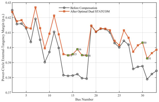
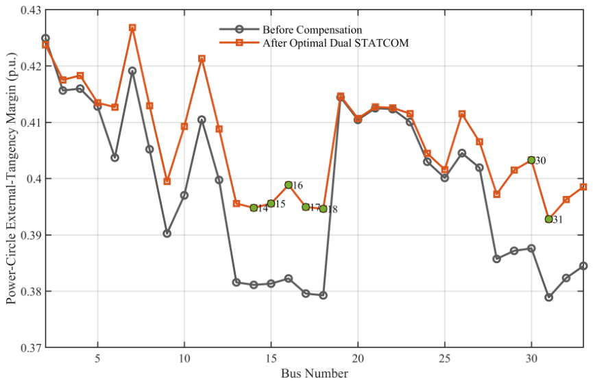
Figure 7 shows that the final dual-STATCOM configuration generally shifts the power-circle margins upward, including the original weak region. This post-compensation result is used as an effectiveness assessment; the power-circle ranking itself is not used to force the optimizer toward Buses 16 or 30.

Figure 7. Power-circle external-tangency margins before and after the deterministic optimal dual-STATCOM compensation.

5.4. Algorithm Performance and Ablation Analysis

The parameter settings of the six compared optimization algorithms are summarized in Table 6. All algorithms use the same population size and iteration budget to ensure a fair comparison.

Table 6. Parameters of the compared optimization algorithms.

Algorithm	Pop.	Iter.	ω	c1	c2	Location/Capacity Encoding	Constraint Handling	Other Settings
SPSO	30	50	0.8	1.5	1.5	Locations: latent [2, 33] + round/repair; Stage 1 Q: 0–10 Mvar, 0.05-Mvar grid; Stage 2 Q: continuous 0–10 Mvar	Deb feasibility rules; no penalty	Velocity clamp: location 8, capacity 3
LDW-PSO	30	50	0.8 → 0.4	1.5	1.5	Same as SPSO	Same as SPSO	Velocity clamp: location 8, capacity 3
TVAC-PSO	30	50	0.8	2.5 → 1.0	1.0 → 2.5	Same as SPSO	Same as SPSO	Velocity clamp: location 8, capacity 3
IPSO	30	50	0.9 → 0.4	2.5 → 1.0	1.0 → 2.5	Same as SPSO	Same as SPSO	Velocity clamp: location 8, capacity 3
GA	30	50	–	–	–	Same location repair and capacity bounds	Deb feasibility rules; no penalty	Arithmetic crossover 0.8; Gaussian mutation 0.10; elite count 2
WOA	30	50	–	–	–	Same location repair and capacity bounds	Deb feasibility rules; no penalty	a: 2 → 0; spiral b = 1

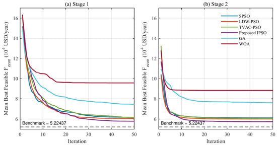
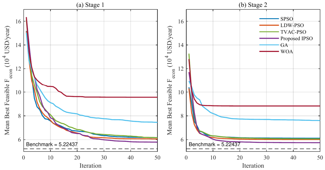
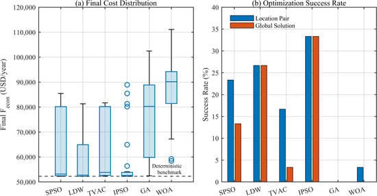
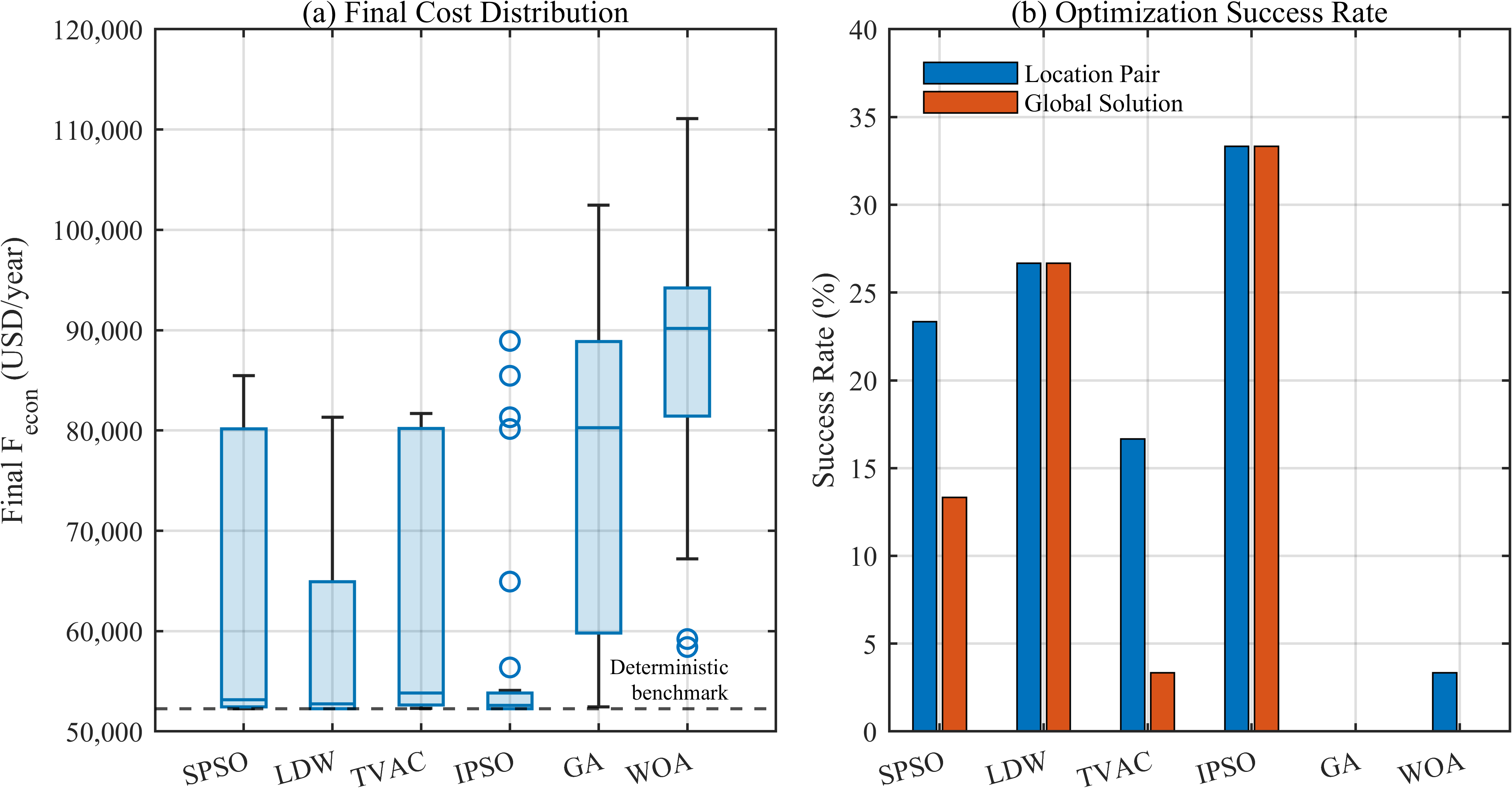
The convergence characteristics of the six algorithms are shown in Figure 8, while the repeated-run statistical results are summarized in Table 7. The corresponding final-cost distributions and optimization success rates are further illustrated in Figure 9.

Figure 8. Mean best-feasible convergence curves for the six algorithms in (a) Stage 1 and (b) Stage 2.

Table 7. Statistical performance over 30 independent runs of the dual-STATCOM problem.

Algorithm	Best Feco (USD/Year)	Mean Feco (USD/Year)	Std.	Worst Feco	Pair Success (%)	Global Success (%)	Runtime (s)	PF evals.	PF Evals. to 0.1% *
SPSO	52,246.47	61,151.78	13,296.72	85,461.77	23.33	13.33	56.12	3000	2640
LDW-PSO	52,243.83	60,082.22	11,819.81	81,305.17	26.67	26.67	55.30	3000	2460
TVAC-PSO	52,287.15	60,605.72	12,375.98	81,693.64	16.67	3.33	55.55	3000	3000
IPSO	52,244.78	57,418.00	10,925.67	88,924.24	33.33	33.33	56.11	3000	2679
GA	52,449.98	76,025.81	14,811.70	102,463.67	0	0	56.33	3000	–
WOA	58,411.12	88,295.51	12,361.00	111,108.85	3.33	0	53.58	3000	–

* “PF evals. to 0.1%” denotes the mean number of power-flow evaluations required, among successful runs, to first reach a feasible objective value within 0.1% of the deterministic benchmark. “–” indicates that no successful run satisfied this criterion.

Figure 9. Statistical algorithm performance: (a) final-cost distributions; (b) optimal-location-pair and global-solution success rates.

The proposed IPSO attains the highest location-pair recovery rate and global-solution success rate, both 33.33% (10/30), as well as the lowest mean F_eco (57,418.00 USD/year) and the smallest standard deviation (10,925.67 USD/year). LDW-PSO reaches the 0.1% optimality threshold with fewer power-flow evaluations among successful runs, so the IPSO advantage is primarily reflected in repeated-run robustness and average solution quality rather than the fastest local convergence.

The ablation results further clarify the contributions of the two adaptive mechanisms. Compared with SPSO, LDW-PSO increases the global-solution success rate from 13.33% to 26.67% and reduces the mean objective value from 61,151.78 to 60,082.22 USD/year, indicating that the decreasing inertia weight improves search robustness. In contrast, TVAC-PSO reduces the global-solution success rate to 3.33%, showing that the time-varying acceleration coefficients alone do not provide a consistent benefit. By combining both mechanisms, the proposed IPSO achieves the highest global-solution success rate of 33.33% and the lowest mean objective value of 57,418.00 USD/year, indicating improved robustness for the dual-STATCOM optimization problem.

A Kruskal–Wallis test across the six final-cost distributions gives p = 5.64 × 10⁻¹⁶. After Holm correction, the proposed IPSO differs significantly from TVAC-PSO (adjusted p = 0.04885), GA, and WOA, with medium-to-large effect sizes, whereas the differences from SPSO and LDW-PSO are not statistically significant. Accordingly, the results support improved robustness on the more complex dual-device problem, but do not justify claiming universal statistical superiority over every PSO baseline.

5.5. Restored N − 1 Line-Outage Voltage Assessment and Required STATCOM Capacity Reinforcement

The N − 1 assessment in this study is limited to restorable single-line outages and steady-state post-restoration voltage compliance. It does not constitute a comprehensive N − 1 security assessment involving generator outages, thermal-loading limits, protection constraints, or dynamic stability. Therefore, the following results are interpreted specifically as post-restoration voltage-compliance performance under single-line contingencies.

The normal-operation economic optimum is next tested under single-line outages. Because the IEEE 33-bus system is radial, each normally closed branch outage is paired with a single normally open tie-line closure to restore a connected radial topology. Of the 32 normally closed branch outages, 31 can be restored by one tie-line operation; the outage of branch 1–2 cannot and is excluded from the post-restoration voltage comparison. The post-restoration voltage-compliance performance of the normal-operation optimal dual-STATCOM configuration is summarized in Table 8.

Table 8. N − 1 robustness of the normal-operation optimal dual-STATCOM configuration.

Metric	NoSTATCOM	OptimalDualSTATCOM	Unit
Restorable contingencies	31 of 32	31 of 32	count
Voltage-compliant contingencies	0	12	count
Voltage-compliance rate	0	38.7100	%
Contingencies with voltage violations	31	19	count
Worst-case Umin	0.7456	0.8250	p.u.
Worst-case DU	6.3178	4.0997	p.u.
Mean Umin improvement	–	0.0402	p.u.
Mean DU improvement	–	35.0600	%
Mean loss reduction	–	30.9827	%
Bus 16 utilization, mean/max	–	100.00/100.00	%
Bus 30 utilization, mean/max	–	100.00/100.00	%
Contingencies at rated capacity, Bus 16/Bus 30	–	31/31	count

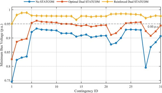
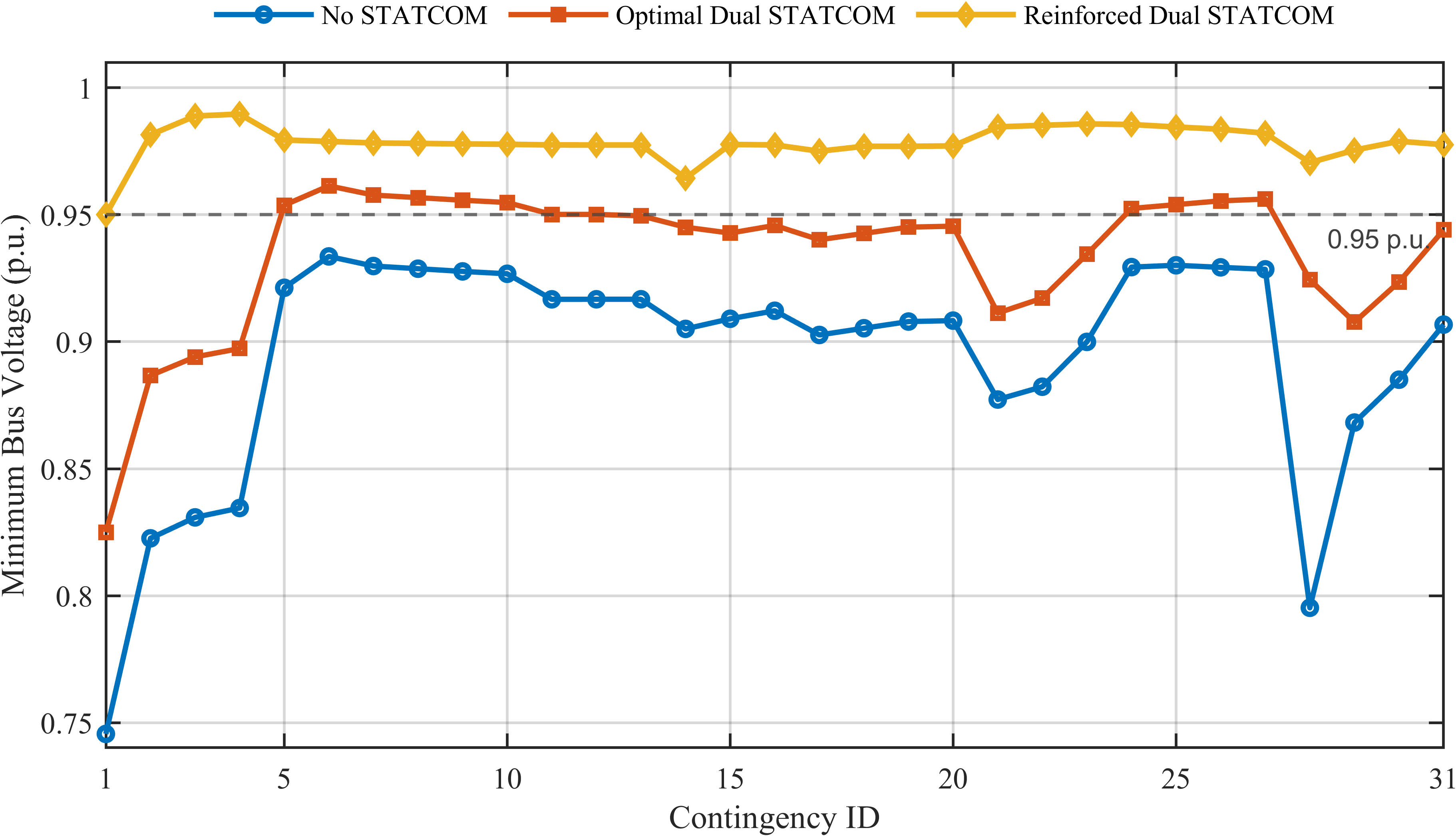
Without STATCOM support, none of the 31 restorable contingencies satisfies the 0.95-p.u. lower-voltage requirement. The normal-operation optimal dual configuration increases the voltage-compliance rate to 38.71% (12/31), raises the worst-case minimum voltage from 0.745611 to 0.825017 p.u., and reduces the mean DU by 35.06% and mean active-power loss by 30.98%. However, both STATCOMs operate at their rated reactive-power limits in all 31 contingencies, so the normal-operation optimum has no remaining reactive-power reserve for severe outages.

To quantify the additional installed capacity required for complete N − 1 voltage compliance, the installation locations are fixed at Buses 16 and 30, and only their ratings are increased. The minimum ratings required to achieve voltage compliance are 1.5423278 Mvar at Bus 16 and 5.0270192 Mvar at Bus 30, for a total of 6.5693470 Mvar. This is 282.96% above the normal-operation optimal total rating and corresponds to a total capacity-reinforcement factor of 3.8296. All 31 restorable contingencies then satisfy the voltage limit within a 10⁻⁹-p.u. numerical tolerance. The binding case is the outage of branch 2–3 restored by tie 21–8, with Bus 25 at the 0.95-p.u. boundary. The minimum bus voltages across the 31 restorable N − 1 contingencies are shown in Figure 10, while the trade-off between the normal-operation economic optimum and the voltage-compliant reinforced dual-STATCOM configuration is summarized in Table 9.

Figure 10. Minimum bus voltage across the 31 restorable N − 1 contingencies for the uncompensated case, the normal-operation optimal dual-STATCOM configuration, and the voltage-compliant reinforced configuration.

Table 9. Trade-off between normal-operation economy and full voltage compliance under restored N − 1 line outages at fixed locations.

Configuration	Q16 Rated (Mvar)	Q30 Rated (Mvar)	Total Rating (Mvar)	Annual Feco (USD/year)	Voltage-Compliance Rate (%)	Worst N − 1 Umin (p.u.)
Normal-operation optimal dual	0.5583	1.1571	1.7154	52,243.71	38.71	0.825017
Voltage-compliant reinforced dual	1.5423	5.0270	6.5693	79,275.96	100.00	0.950000

The reinforced configuration increases annual cost by 27,032.25 USD/year (51.74%) relative to the normal-operation dual optimum. In the base topology, its active-power loss and D_U are numerically unchanged because the additional installed capacity need not be dispatched under normal conditions; the cost increase is therefore associated with the larger rated capacity. This result distinguishes economic planning for normal operation from security-constrained capacity planning.

6. Conclusions

This study reformulated STATCOM planning on the IEEE 33-bus radial distribution system so that electrical-vulnerability assessment, economic siting/sizing, algorithm validation, and contingency evaluation are treated as distinct but complementary tasks.

(1)

The power-circle-based external-tangency margin consistently identifies electrically vulnerable regions across the tested loading levels and shows substantial ranking agreement with Q–V continuation-power-flow results. Specifically, the rankings remain highly correlated over the 0.8–1.2 loading range, while the comparison with Q–V analysis yields a Spearman correlation of 0.8644 and a 90% Top-10 overlap. These results support the use of the power-circle margin as a comparative vulnerability indicator and post-compensation assessment metric, rather than as a direct quantitative measure of voltage-stability margin.

(2)

Deterministic benchmarking shows that the best single STATCOM is 3.6689 Mvar at Bus 7, whereas the best dual configuration is 0.5583 Mvar at Bus 16 and 1.1571 Mvar at Bus 30. The dual solution reduces installed capacity by 53.24% and annual cost by 38.86% relative to the optimal single-device solution, while reducing active-power loss to 0.1402 MW and satisfying all normal-operation voltage constraints.

(3)

On the 496-pair dual-location problem, the proposed two-stage IPSO achieves the highest location-pair and global-solution success rates (33.33%), and the lowest mean objective value over 30 independent runs among the six compared algorithms. Its advantage is mainly in search robustness and average solution quality; pairwise statistical tests do not support a claim of significant superiority over every PSO baseline.

(4)

The normal-operation economic optimum improves restored N − 1 voltage performance but does not guarantee complete N − 1 security because both STATCOMs saturate in severe contingencies. With the locations fixed, full compliance for all 31 restorable contingencies requires a total rating of 6.5693 Mvar and raises annual cost by 51.74%. This quantifies the practical trade-off between normal-operation economy and contingency-required STATCOM capacity.

Future work will extend the planning model to multi-period loading and renewable-generation uncertainty, incorporate fixed per-device installation costs, and directly co-optimize normal-operation economy and contingency-security constraints.

References

- Sirjani, R.; Rezaee Jordehi, A. Optimal placement and sizing of distribution static compensator (D-STATCOM) in electric distribution networks: A review. Renew. Sustain. Energy Rev. 2017, 77, 688–694. [Google Scholar] [CrossRef] [Scilit]
- Valencia-Díaz, A.; García Hoyos, S.; Hincapié Isaza, R.A. Stochastic optimization for siting and sizing of renewable distributed generation and D-STATCOMs. e-Prime Adv. Electr. Eng. Electron. Energy 2025, 13, 101026. [Google Scholar] [CrossRef] [Scilit]
- Alanazi, A.; Alanazi, M.; Memon, Z.A.; Awan, A.B.; Deriche, M. Availability and uncertainty-aware optimal placement of capacitors and DSTATCOM in distribution network using improved exponential distribution optimizer. Sci. Rep. 2025, 15, 13204. [Google Scholar] [CrossRef] [Scilit] [PubMed]
- Tejaswini, V.; Susitra, D. Optimal D-STATCOM placement and sizing using a novel bird swarm operated exploitation of elephant herd algorithm. Sci. Rep. 2025, 15, 13563. [Google Scholar] [CrossRef] [Scilit] [PubMed]
- Montoya, O.D.; Grisales-Noreña, L.F.; Gil-González, W. Simultaneous siting and sizing of PVs and D-STATCOMs in medium-voltage grids using the Cauchy-based distribution optimizer. Results Eng. 2025, 25, 104407. [Google Scholar] [CrossRef] [Scilit]
- Cubillo-Leyton, P.I.; Montoya, O.D.; Grisales-Noreña, L.F. Optimized integration of photovoltaic systems and distribution static compensators in distribution networks using a novel discrete-continuous version of the adaptive JAYA algorithm (AJAYA). Results Eng. 2025, 26, 104726. [Google Scholar] [CrossRef] [Scilit]
- Suárez Patiño, J.E.; Gallego Pareja, L.A.; Gomez-Carmona, O. Optimal placement, sizing and operation of D-STATCOMs in power distribution systems using a Mixed-Integer Linear Programming model. Results Eng. 2025, 26, 104749. [Google Scholar] [CrossRef] [Scilit]
- Yenealem, M.G. Optimum allocation of microgrid and D-STATCOM in radial distribution system for voltage profile enhancement using particle swarm optimization. Int. J. Photoenergy 2024, 2024, 5550897. [Google Scholar] [CrossRef] [Scilit]
- Montoya, O.D.; Ramírez-Vanegas, C.A.; Grisales-Noreña, L.F. A Sine-Cosine Algorithm approach for optimal PV and D-STATCOM integration in distribution systems. Stat. Optim. Inf. Comput. 2025, 13, 1266–1279. [Google Scholar] [CrossRef] [Scilit]
- Colot, A.; Perotti, E.; Glavic, M.; Dall’Anese, E. Incremental Volt/Var control for distribution networks via chance-constrained optimization. IEEE Trans. Power Syst. 2025, 40, 4561–4573. [Google Scholar] [CrossRef] [Scilit]
- Xiong, K.; Cao, D.; Zhang, G.; Chen, Z.; Hu, W. Coordinated Volt/VAR control for photovoltaic inverters: A soft actor-critic enhanced droop control approach. Int. J. Electr. Power Energy Syst. 2023, 149, 109019. [Google Scholar] [CrossRef] [Scilit]
- Montoya, O.D.; Gil-González, W.; Garcés, A. An energy management system for PV-STATCOMs in power distribution networks via a complex-domain SDP relaxation. Energy Syst. 2025, 17, 1–16. [Google Scholar] [CrossRef] [Scilit]
- Roy, N.K.; Pota, H.R.; Hossain, M.J. Reactive power management of distribution networks with wind generation for improving voltage stability. Renew. Energy 2013, 58, 85–94. [Google Scholar] [CrossRef] [Scilit]
- Sharma, P.; Mohapatra, A.; Sharma, A. Power circle diagrams and aggregate flexibility curves for active distribution networks. Electr. Power Syst. Res. 2022, 206, 107820. [Google Scholar] [CrossRef] [Scilit]
- Salama, H.S.; Vokony, I. Voltage stability indices—A comparison and a review. Comput. Electr. Eng. 2022, 98, 107743. [Google Scholar] [CrossRef] [Scilit]
- Tahir, M.J.; Bakar, B.A.; Alam, M.; Mazliham, M.S. A comprehensive review: Optimal capacitor placement and sizing in a distribution system. J. Eng. Technol. 2018, 6, 31–36. [Google Scholar]
- Alemu, A.T.; Meseret, G.M. Optimal Location and Sizing of Static Var Compensator (SVC) to Improve Voltage Profile in Distribution Network. Eng. Rep. 2025, 7, e70435. [Google Scholar] [CrossRef] [Scilit]
- Kennedy, J.; Eberhart, R. Particle swarm optimization. In Proceedings of the IEEE International Conference on Neural Networks (ICNN’95), Perth, Australia, 27 November–1 December 1995; Volume 4, pp. 1942–1948. [Google Scholar]
- Shi, Y.; Eberhart, R.C. A modified particle swarm optimizer. In Proceedings of the IEEE International Conference on Evolutionary Computation, Anchorage, AK, USA, 4–9 May 1998; pp. 69–73. [Google Scholar]
- Ratnaweera, A.; Halgamuge, S.K.; Watson, H.C. Self-organizing hierarchical particle swarm optimizer with time-varying acceleration coefficients. IEEE Trans. Evol. Comput. 2004, 8, 240–255. [Google Scholar] [CrossRef] [Scilit]
- Clerc, M.; Kennedy, J. The particle swarm—Explosion, stability, and convergence in a multidimensional complex space. IEEE Trans. Evol. Comput. 2002, 6, 58–73. [Google Scholar] [CrossRef] [Scilit]
- Eberhart, R.C.; Shi, Y. Particle swarm optimization: Developments, applications and resources. In Proceedings of the 2001 Congress on Evolutionary Computation, Seoul, Republic of Korea, 27–30 May 2001; Volume 1, pp. 81–86. [Google Scholar]
Disclaimer/Publisher’s Note: The statements, opinions and data contained in all publications are solely those of the individual author(s) and contributor(s) and not of MDPI and/or the editor(s). MDPI and/or the editor(s) disclaim responsibility for any injury to people or property resulting from any ideas, methods, instructions or products referred to in the content. |
© 2026 by the authors. Licensee MDPI, Basel, Switzerland. This article is an open access article distributed under the terms and conditions of the Creative Commons Attribution (CC BY) license.