Flow-Loop Investigation and DAS-Based Flow-Rate Prediction for Gas–Water Two-Phase Flow Under Near-Horizontal High-Rate Gas-Well Conditions

Abstract

Gas–water two-phase flow at high gas rates and low water cuts generates complex acoustic responses, necessitating experimental calibration for distributed acoustic sensing (DAS)-based flow-rate estimation. Near-horizontal air–water flow-loop experiments were conducted at well inclinations of 85°, 88°, and 90°, covering different flow-rate and water-cut combinations. Spectral analysis showed that DAS signal energy was concentrated below 500 Hz. Four flow regimes were identified: bubbly, slug, stratified, and wavy flow. Flow-regime-dependent characteristic Reynolds numbers (Re) were correlated with frequency-band energy (FBE), and the fitted coefficients were compiled into a database. For each inclination, Gaussian process regression was used for coefficient interpolation within the calibration range, while Bayesian ridge regression enabled limited extrapolation near the calibration boundaries. Measured FBE and reconstructed Re–FBE relationships were used to estimate characteristic Reynolds numbers and calculate total flow rates. Across 26 independent validation conditions, absolute relative errors ranged from 0.05% to 8.98%, with a mean absolute percentage error of 3.01%, compared with 18.28% for cross-correlation. These results support quantitative DAS-based flow-rate estimation under the tested laboratory conditions. Application to actual gas wells requires further calibration and validation under representative high-temperature and high-pressure conditions.

1. Introduction

Monitoring flow rate and phase distribution in gas–water two-phase flow is essential for evaluating gas-well production performance and interpreting production profiles. In near-horizontal wells, changes in flow rate, water cut, and well inclination affect phase distribution and interfacial motion, complicating quantitative interpretation. Distributed acoustic sensing (DAS) provides an alternative means of monitoring multiphase flow in wellbores [1]. It uses Rayleigh backscattering in optical fibers and phase-sensitive optical time-domain reflectometry (Φ-OTDR) to detect and locate mechanical vibrations along the sensing fiber. When combined with distributed temperature sensing (DTS), DAS enables complementary measurements of wellbore conditions [2]. Distributed fiber-optic sensing has been applied to reservoir surveillance, completion evaluation, hydraulic-fracturing monitoring, and production monitoring [1,2,3].

For wellbore flow monitoring, Panhuis et al. [4] investigated applications of DAS to zonal production and injection allocation, fluid-transport tracking, and flow diagnostics, primarily in liquid-producing and injection wells. Their work demonstrated the feasibility of distributed fiber-optic sensing for flow monitoring and production-profile interpretation. Zett et al. [5] addressed the non-uniqueness of DTS interpretation in complex completions by calibrating temperature models against conventional production-logging data. Sensitivity analyses showed that different inflow distributions could produce similar temperature profiles. They also conducted horizontal air–water slug-flow experiments to compare DAS and array production-logging responses under different fiber configurations and examined the use of acoustic information to constrain possible flow scenarios. For hydraulic-fracturing monitoring, Karrenbach et al. [6] recorded DAS microseismic signals in field experiments and investigated their integration with temperature and strain measurements. These studies established a basis for detecting wellbore flow events and extracting flow-related information from DAS measurements.

For velocity estimation and production allocation, Jin et al. [7] developed a joint DAS–DTS interpretation approach for low-rate oil producers. DTS provided temperature measurements, whereas low-frequency DAS tracked transient thermal disturbances to estimate velocity. A Markov chain Monte Carlo inversion was then used to obtain production allocations consistent with both temperature and velocity observations. The approach was evaluated using a single-phase water flow loop, synthetic models, and field examples. Titov et al. [8] conducted single-phase liquid and gas–liquid experiments in a vertical flow loop, using DAS to track thermal slugs for velocity estimation and multiphase-flow characterization. These studies advanced fiber-optic monitoring from flow-event detection towards quantitative interpretation of flow parameters.

For flow-rate prediction based on acoustic features, Tabjula et al. [9] extracted root-mean-square amplitudes and frequency-band energies from DAS measurements of single-phase water and synthetic oil-based drilling fluids. They established linear, exponential, and cubic empirical correlations and performed blind validation using wellbore and surface flow-loop datasets. For two-phase flow structures, Ali et al. [10] conducted horizontal air–mineral-oil slug-flow experiments. By identifying and tracking slug signatures in low-frequency DAS signals, they estimated slug frequency, translational velocity, and characteristic lengths of liquid slugs, slug units, and liquid-film regions, with validation against high-speed imaging. Zeng et al. [11] developed a full-scale DAS flow-monitoring facility based on the completion configuration and reservoir conditions of the FBH well. Single-phase gas and gas–water experiments supported field interpretation of producing intervals, thermal-front tracking during well opening, and liquid backflow during shut-in. Early-time production was also estimated from thermal-front trajectories. Luo et al. [12] conducted horizontal gas–water flow experiments and established regression-based relationships between DAS acoustic energy and wellbore flow velocity, providing an experimental basis for acoustic flow-rate estimation.

Therefore, existing approaches include acoustic constraints on flow interpretation, thermal-feature tracking, slug-structure characterization, and empirical correlations based on acoustic features. Each has specific requirements. Qualitative acoustic constraints can reduce interpretation ambiguity but require additional quantitative relationships for flow-rate estimation. Thermal-feature tracking depends on identifiable temperature disturbances and suitable transport conditions. Slug-parameter extraction requires recognizable flow structures and a relationship between their propagation velocity and the total gas–liquid flow rate. Empirical correlations depend on the calibration fluids, operating conditions, and measurement configuration; relationships established for single-phase flow or specific conditions cannot be transferred directly to other gas–water flow conditions. Although acoustic energy–velocity calibration has been investigated for gas–water flow, further work is required under near-horizontal, high-gas-rate, and low-water-cut conditions. In particular, the effects of inclination and water cut on calibration relationships should be assessed under consistent experimental and processing conditions, together with prediction performance at conditions not directly included in the calibration. Field application also requires clearly defined pressure and temperature references for phase flow rates and consideration of changes in fluid properties and fiber coupling [13,14].

Accordingly, this study uses a large-diameter flow-loop facility to investigate DAS spectra and frequency-band energy under near-horizontal gas–water flow conditions. Characteristic Reynolds numbers are selected based on observed flow regimes, and empirical Re–FBE relationships are established to construct a coefficient database. GPR is used for coefficient interpolation within the calibration range, whereas BRR is used for limited extrapolation near the calibration boundaries. The predicted coefficients are combined with measured FBE to estimate flow rate. Prediction errors are evaluated using high-gas-rate, low-water-cut validation conditions and compared with those obtained using the cross-correlation method.

2. Experimental Scheme

Motivated by the production characteristics of high-rate gas wells in the Fuling shale gas field, flow-loop experiments were conducted to investigate near-horizontal gas–water flow. A DAS system recorded the acoustic responses under different flow-rate and water-cut conditions, with particular emphasis on high gas rates and low water cuts. The experiments examined the relationship between pipeline flow rate and the measured DAS response.

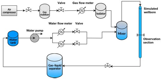
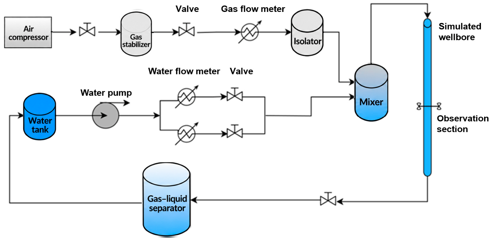
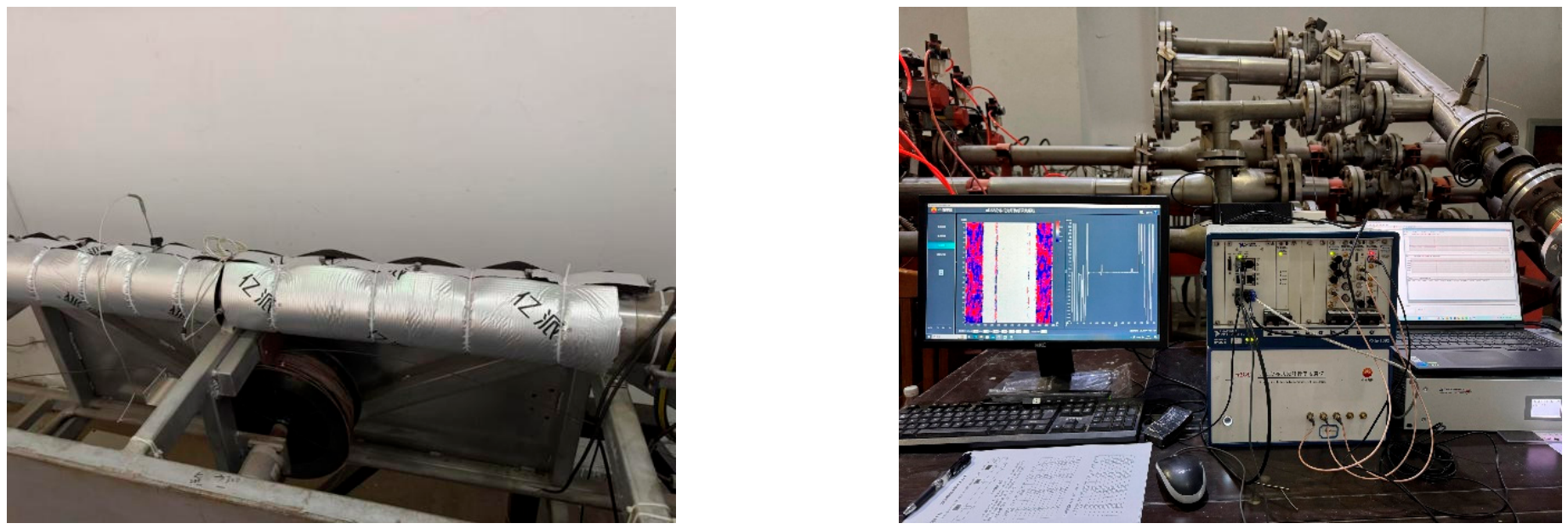
Figure 1 shows the components and flow paths relevant to the present experiments, including the gas–liquid separator, stabilizer, air compressor, gas and water flowmeters, isolator, mixer, valves, and test section. The test section was 10 m long and had an inner diameter of 115 mm, comprising a transparent observation section and a metal section. The observation section was located 3 m downstream of the inlet, equivalent to approximately 26.1 pipe diameters. The internal diameters of the inlet and outlet flow passages were 20 and 50 mm, respectively. Data were recorded after stable operation was established to reduce the effects of start-up and flow-rate adjustment. Flow regimes were identified from videos of the observation section, and the identified regime remained unchanged during each recording period. DAS measurements were acquired using the uDAS system developed by BGP Borehole Division, at a sampling frequency of 2000 Hz and a spatial sampling interval of 0.1 m. The sensing fiber was helically wound around the outer pipe wall at an axial spacing of 0.25 m. Acoustic insulation was applied around the metal section to reduce external noise and provide thermal insulation, as illustrated in Figure 2.

Figure 1. Schematic diagram of the flow-loop experimental setup.

Figure 2. Schematic diagram of the DAS experimental setup. (left) Fiber installation and outer sound-insulating cotton layer used in the experiments. (right) uDAS data acquisition system.

Tap water and air were used as the liquid and gas phases, respectively. Single-phase gas, single-phase water, and gas–water two-phase experiments were conducted near room temperature and atmospheric pressure at different inclination angles, with particular emphasis on high-gas-rate, low-water-cut conditions. The inclination angles, flow rates, and water cuts are summarized in Table 1.

Table 1. Gas–water flow-rate combinations.

Well inclination (o)	90, 88, 85
Total flow rate (m3/d)	50, 60, 100, 120, 160, 200, 300, 500, 1000, 4000, 9000, 10,000, 14,000, 18,000, 20,000, 24,000, 5000, 5469, 8313, 9368, 10,000, 16,152, 16,819, 19,382, 20,000, 22,000
Water cut (%)	0, 1, 10, 30, 50, 70, 90, 100, 0.5, 0.75, 1.5, 2, 3, 4, 0.45, 0.68, 0.9

The gas and water flow rates reported in this study are volumetric flow rates referenced to the actual temperature and pressure in the test section. Water cut, C_w, is defined as the ratio of the water volumetric flow rate to the total gas–water volumetric flow rate at the same temperature and pressure.

$$C_w={\displaystyle \frac{Q_w}{Q_w+Q_g}}$$

(1)

Here, Q_w and Q_g denote the water and gas volumetric flow rates converted to the actual test-section conditions. The experimental temperature ranged from 294.15 to 308.15 K, and the absolute pressure in the test section was taken as 101.325 kPa. The superficial velocity of each phase was calculated by dividing its volumetric flow rate by the total pipe cross-sectional area. The gas and water superficial velocities ranged from 0 to 26.743 m/s and from 0 to 0.334 m/s, respectively. The inclination angles and phase flow-rate combinations were selected to investigate flow scenarios relevant to near-horizontal gas wells. The experiments were intended to examine the DAS response–flow-rate relationship under the selected conditions and were not designed to reproduce actual gas wells according to complete dynamic-similarity criteria.

3. Data Processing and Analysis

3.1. Data Processing

Each DAS data file contained a 6 s recording, with rows representing spatial channels and columns representing time samples. For each spatial channel, 160 consecutive time samples were selected as the analysis segment, corresponding to a duration of 0.08 s. Mean removal, linear detrending, and Hann windowing were applied sequentially, followed by a 160-point fast Fourier transform (FFT) along the time axis. No zero-padding, sliding segmentation, or overlapping analysis windows were used. The frequency-bin spacing was 12.5 Hz. The processing steps are described below.

3.1.1. Signal Mean Removal

The signal mean was removed to eliminate the constant offset and prevent a dominant zero-frequency peak from obscuring other spectral components.

3.1.2. Detrending

Linear detrending removes the linear trend from the signal, preventing slowly varying components from introducing low-frequency artifacts into the spectrum and obscuring the underlying signal characteristics.

3.1.3. Windowing

A Hann window was applied to the analysis segment to reduce spectral leakage caused by signal truncation.

3.1.4. Frequency-Band Energy

For file j, spatial channel c, and frequency band b, the band-energy statistic was calculated from the squared magnitudes of the FFT coefficients within that band.

$$E_{j,c,b}=\sum _{k\in {\kappa }_b}{\displaystyle \frac{{\left|X_{j,c}\left[k\right]\right|}^2}{N}}$$

(2)

$${\kappa }_b=\left\{k:f_b^l\le f_k<f_b^U\right\}$$

(3)

The frequency bands were defined using inclusive lower bounds and exclusive upper bounds. The squared FFT magnitudes were normalized by the number of samples, N, without compensation for the Hann-window energy.

$$\overline{E_b}={\displaystyle \frac{1}{J}}{\displaystyle \sum _{j=1}^J}\left({\displaystyle \frac{1}{C_j}}{\displaystyle \sum _{c=1}^{C_j}}{E}_{j,c,b}\right)$$

(4)

$$\mathit{FBE}=\mathit{max}\overline{E_b}(\mathrm{a}.\mathrm{u}.)$$

(5)

The band-energy statistics were first averaged across spatial channels within each file and then averaged with equal weighting across files corresponding to the same operating condition. The maximum of the resulting band-averaged values was used as the scalar FBE predictor for subsequent modeling. FBE is reported in arbitrary units (a.u.).

3.2. Analysis of Experimental Results

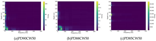
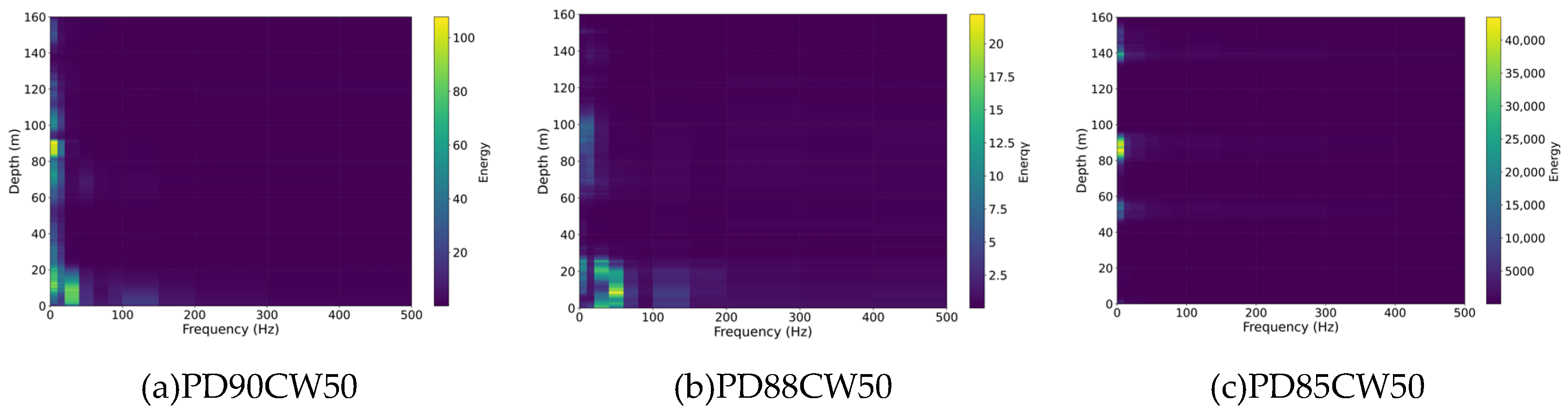
Based on the procedures above, spectral analysis was performed on the DAS data obtained under different operating conditions. The results are shown in Figure 3.

Figure 3. Waterfall plot of frequency-band energy. (a) Energy waterfall plot at a well inclination of 90° and a water cut of 50%. (b) Energy waterfall plot at a well inclination of 88° and a water cut of 50%. (c) Energy waterfall plot at a well inclination of 85° and a water cut of 50%.

Taking a water cut of 50% as an example, the horizontal axis in the figure represents frequency, while the vertical axis represents depth. The color shifts toward yellow as signal intensity increases. The figure shows the following features:

(1) The DAS signal energy in the near-horizontal gas–water flow experiments was concentrated primarily below 500 Hz, with the strongest response below 100 Hz.

(2) The spatial continuity of the DAS energy response decreased as the inclination angle decreased from 90°. At 90°, the response generally exhibited continuous bands along the test section, possibly reflecting spatial coherence in water-phase wall interactions and interfacial fluctuations. At 88° and 85°, the response became more localized and patch-like, indicating greater spatial heterogeneity. This change may be associated with a redistribution of the dominant excitation regions and less spatially coherent interactions between the water phase and the pipe wall.

On this basis, frequency-band energy–frequency curves of DAS signals under different operating conditions were also plotted, as shown in Figure 3.

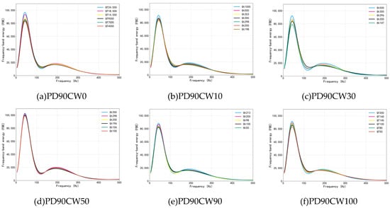
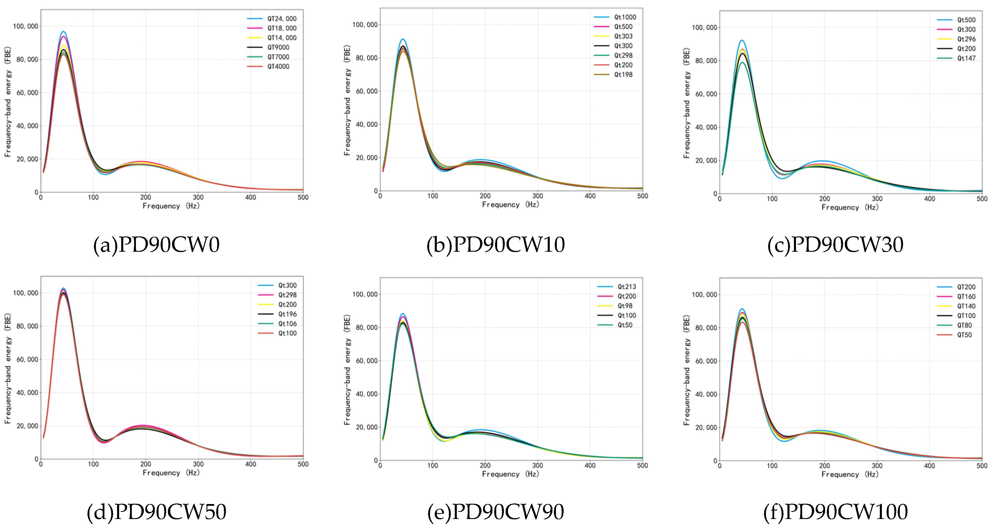
Figure 4 presents the frequency-band energy–frequency curves for six operating conditions at an inclination angle of 90°. Frequency and band energy are plotted on the horizontal and vertical axes, respectively. Joint examination of Figure 3 and Figure 4 reveals the following features.

Figure 4. Frequency-band energy–frequency curves at PD90. (a–f) Frequency–FBE curves at a well inclination of 90° and water cuts of 0%, 10%, 30%, 50%, 90%, and 100%, respectively.

(1) The frequency-band energy–frequency curves exhibited dominant peaks within 0–100 Hz under all investigated conditions, confirming that the DAS response was dominated by low-frequency components, consistent with the preceding spectral analysis. Energy generally decreased with increasing frequency, although local peaks remained in some bands. The low-frequency response may be associated with gas–water interfacial motion and large-scale flow disturbances; however, the contributions of different disturbances require further investigation using synchronized flow observations.

(2) The dominant peaks occurred at similar frequencies under different flow-rate and water-cut conditions. Within the operating range and frequency resolution of the present experiments, no pronounced peak-frequency shift was observed, whereas changes in peak magnitude were more apparent. Energy magnitude therefore provided a more useful basis than peak frequency for distinguishing the investigated flow conditions.

(3) At the same inclination angle and water cut, the frequency-band energy at the dominant peak increased with flow rate, indicating an enhanced low-frequency vibration response. This trend may be associated with changes in flow disturbances and fluid–wall interactions as flow rate increases. Under gas–water two-phase conditions, interfacial motion associated with flow structures may also contribute to the measured response [15]. However, the present measurements cannot distinguish the contributions of different excitation sources and transmission processes. Therefore, no further conclusions are drawn regarding the relative energy-transfer efficiencies of low- and high-frequency disturbances.

(4) Under the comparable conditions shown in the figure, the energy response first increased and then decreased with increasing water cut, exhibiting a relatively strong response near the tested water cut of 50%. Differences in gas and water properties, together with the formation of the gas–water interface and disturbances associated with local flow structures, may contribute to this trend [16].

(5) At the same flow rate and water cut, the DAS frequency-band energy generally decreased as the well inclination decreased from 90° to 88° and 85°, indicating that inclination changes within the near-horizontal range affected the measured response. This trend may be associated with the helically wound fiber configuration used in the present experiments [17], which enhances sensitivity to radial strain compared with a straight axial fiber installation [18]. Under horizontal conditions, pronounced gas–water stratification results in predominantly shear-driven fluid–wall interactions [19]. The dominance of tangential stresses may therefore produce a stronger axial strain response. As the inclination decreases, gravitational segregation may weaken, and fluid-induced loading may increasingly involve normal impacts and radial compression, resulting in a transition from predominantly axial deformation to coupled deformation in multiple directions. Although the radial response may increase at lower inclination angles, the greater sensitivity of DAS to strain along the fiber axis may lead to a reduction in the overall effective strain response, manifested as lower measured DAS energy.

Overall, the DAS signal energy in the present experiments was concentrated primarily below 500 Hz, with dominant peaks within 0–100 Hz. Peak frequencies varied relatively little across operating conditions, whereas differences in energy magnitude were more pronounced. Within the investigated conditions, increasing flow rate generally corresponded to higher dominant-peak energy. The energy response varied non-monotonically with water cut, exhibiting a relatively strong response near 50% water cut. Frequency-band energy generally decreased as the inclination angle decreased from 90° to 85°. These distinct variations in DAS frequency-band energy across inclination angles and operating conditions provide a basis for developing an FBE-based flow-rate prediction model.

3.3. Flow-Rate Prediction Model

To improve the reliability of model predictions when the target water cut differs from those represented in the calibration data, it is necessary to identify a characteristic parameter that is strongly correlated with fluid velocity but also shows a clear correspondence with frequency-band energy. The Reynolds number, which integrates fluid density, velocity, pipe size, and viscosity, is essentially a dimensionless scale used to describe flow characteristics [20]. It also has a clear physical coupling relationship with frequency-band energy, which makes it highly suitable for model construction. Therefore, the Reynolds number was selected as the optimal parameter for the prediction model. It is expressed as follows:

$$\mathit{Re}={\displaystyle \frac{G\cdot D}{\mu }},$$

(6)

where G = ρ·v; ρ is the density (kg/m³); v is the superficial velocity (m/s); D is the pipe diameter (m); and μ is the effective viscosity (Pa·s). In addition, since complex flow-regime transitions occur during gas–water two-phase flow in near-horizontal wells, the effect of different flow regimes on Reynolds number calculation was further considered in this study. Based on analysis of the experimental videos, the flow regimes under different operating conditions at the three well inclinations were classified. Four main flow regimes were observed in the experiment: bubbly flow, slug flow, stratified flow, and wavy flow [21,22].

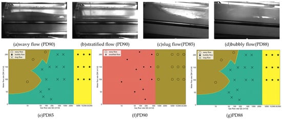
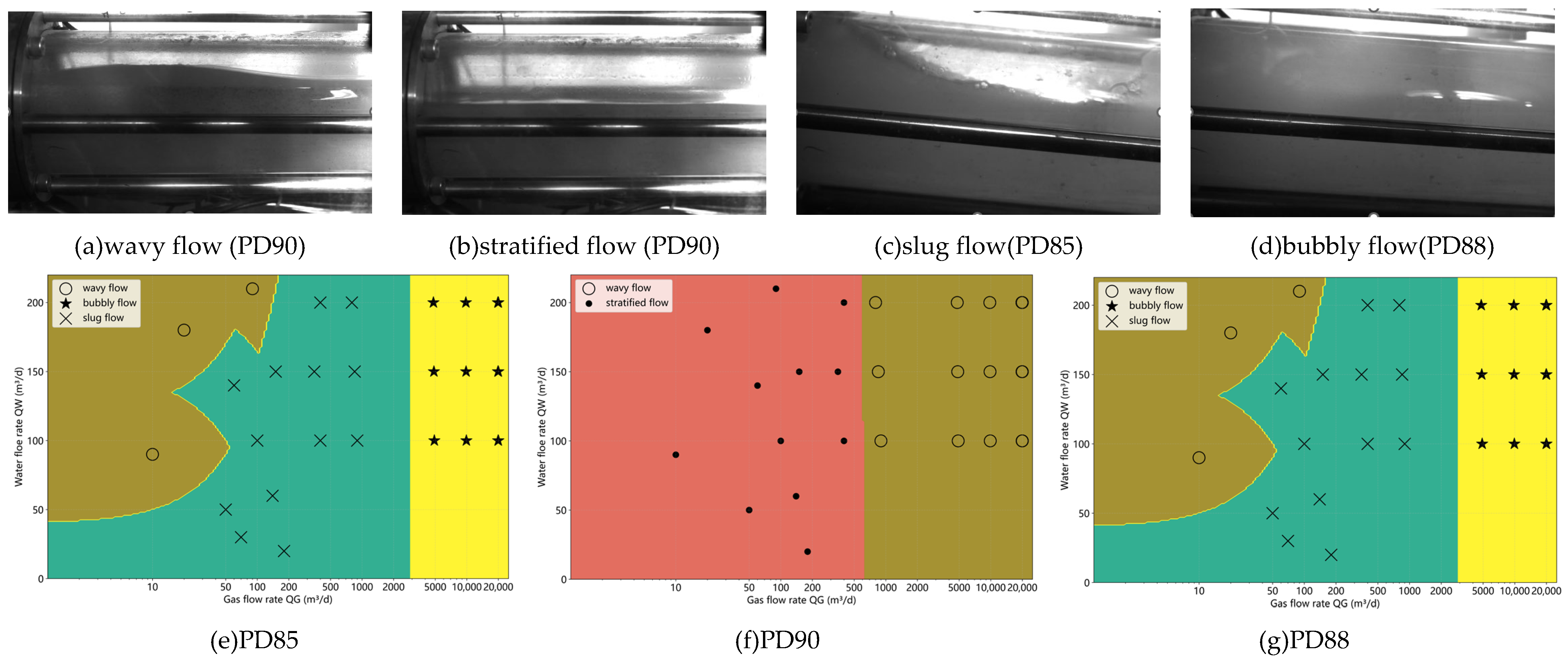
The upper part of Figure 5 presents representative flow regimes observed during the experiments, while the lower part shows gas–water flow-regime maps constructed from these observations. Flow regimes were identified using the following visual criteria. Bubbly flow was characterized by bubbles substantially smaller than the pipe inner diameter and uniformly dispersed within the water phase. Slug flow was identified by elongated Taylor bubbles occupying nearly the entire pipe cross-section and separated by liquid slugs. Stratified flow was characterized by stable segregation of the gas and water phases into the upper and lower portions of the pipe, respectively. Within the stratified-flow category, a smooth interface without visually discernible waves and a steady flow appearance was classified as smooth stratified flow, referred to here as stratified flow. A visibly undulating interface accompanied by flow disturbances was classified as stratified wavy flow, referred to here as wavy flow.

Figure 5. Flow-regime distribution map of gas–water two-phase flow. (a) Wavy flow was observed primarily at a well inclination of 90° and in the low-flow-rate ranges at inclinations of 88° and 85°. (b) Stratified flow was observed primarily in the low-to-moderate flow-rate range at a well inclination of 90°. (c) Slug flow was observed primarily in the high-flow-rate range at well inclinations of 88° and 85°. (d) Bubbly flow was observed primarily in the low-to-moderate flow-rate range at well inclinations of 88° and 85°. (e–g) Flow-regime map constructed from experimentally observed flow regimes.

Because phase distributions and momentum-transfer mechanisms differ among flow regimes, different characteristic Reynolds-number definitions were adopted to relate DAS frequency-band energy to the dominant flow mechanisms.

First, under bubbly flow conditions, the gas phase is dispersed in the continuous water phase in the form of small bubbles. The interphase slip effect is weak, and the overall flow exhibits approximately homogeneous mixture characteristics. In this case, the two-phase flow can be treated as a single equivalent mixed fluid, and the mixture Reynolds number can be used to characterize the flow state [23,24].

$$R{e}_m={\displaystyle \frac{{\rho }_m\cdot v_m\cdot D}{{\mu }_m}},$$

(7)

where v_m is the mixture velocity (m/s);

v_m = v_sg + v_sw,

(8)

where ρ_m is the mixture density (kg/m³) and μ_m is the mixture viscosity (Pa·s).

ρ_m = C_gρ_g + (1 − C_g)ρ_w,

(9)

$${\mu }_m={\mu }_g^{C_g}{\mu }_w^{1-C_g}.$$

(10)

Here, C_g denotes the gas volumetric flow fraction, with both gas and water volumetric flow rates referenced to the actual temperature and pressure in the test section. It was calculated from the imposed phase flow rates and does not represent an independently measured in situ gas holdup. The homogeneous no-slip approximation was applied only under bubbly flow conditions, with C_g used to calculate the effective mixture properties. Fluid properties were determined according to the experimental temperature, pressure, and working fluids to calculate the characteristic Reynolds number. The air density under the experimental conditions was estimated using the following equation of state:

$${\rho }_g={\displaystyle \frac{P}{Z{R}_{g}T}},$$

(11)

where Z is the gas compressibility factor; P is the absolute pressure (Pa); R_g is the gas constant, J/(kg·K); and T is the absolute temperature (K). The water-phase density was assumed to remain constant within the temperature, pressure, and salinity ranges investigated, because its variation had a negligible effect on the Reynolds number and the resulting flow-rate predictions. When the wellbore temperature, pressure, or formation-water salinity varies substantially, the water-phase density should be adjusted according to the actual operating conditions. In addition, during model development, the gas compressibility factor was taken as Z = 1 for the experiments conducted near room temperature and at atmospheric pressure. This approximation is not directly applicable to high-pressure natural gas.

Sensitivity analysis showed that the relative variation in fluid viscosity was greater than that in fluid density [25]; consequently, viscosity variations had a more pronounced effect on the calculated Reynolds number. Further comparison indicated that, under the experimental conditions, variations in gas-phase viscosity had negligible effects on the Reynolds number and flow-rate predictions. Therefore, the gas-phase viscosity was approximated as a constant (μ_g = 1.85 × 10⁻⁵ Pa∙s), whereas the water-phase viscosity was calculated as a function of the wellbore temperature:

$${\mu }_w=a\times {10}^{{\displaystyle \frac{b}{T-c}}},$$

(12)

where a = 2.414 × 10⁻⁵, b = 247.8, and c = 140. The mixture Reynolds number characterizes the relative importance of inertial and viscous effects under bubbly flow conditions and serves as an intermediate physical parameter linking the DAS response to flow rate.

Second, for slug flow, the experimental observations showed that liquid slugs and elongated gas bubbles or gas pockets were alternately distributed along the pipe axis, resulting in pronounced flow intermittency. Under these conditions, the pipe wall was predominantly in contact with the water phase in both the liquid-slug regions and the liquid-film regions surrounding the elongated gas bubbles. Consequently, the water phase made the dominant contribution to the wall shear stress, whereas the gas slugs primarily induced pressure fluctuations and low-frequency flow disturbances rather than directly contributing to momentum transfer at the pipe wall. Because DAS signals can capture the pressure fluctuations and low-frequency flow disturbances induced by gas-slug motion, mixture properties were not used to characterize slug flow in this study. Instead, the water-phase Reynolds number was employed to characterize the flow state under slug-flow conditions:

$$R{e}_w={\displaystyle \frac{{\rho }_w\cdot v_{\mathit{sw}}\cdot D}{{\mu }_w}},$$

(13)

where ρ_w is the water-phase density (kg/m³); μ_w is the water-phase viscosity (Pa·s); and v_sw is the water superficial velocity (m/s).

$$v_{\mathit{sw}}={\displaystyle \frac{Q_w}{A}}.$$

(14)

This definition characterizes the relative importance of inertial and viscous effects in the continuous water phase under slug-flow conditions and serves as an auxiliary parameter for describing water-phase-dominated wall shear behavior. The pressure fluctuations, interfacial disturbances, and intermittent-flow characteristics induced by gas-slug motion are primarily captured by the DAS signals. Therefore, integrating the water-phase Reynolds number with the DAS signal features accounts for the effects of continuous water-phase flow and intermittent gas-slug disturbances on the signal response simultaneously, thereby enabling the development of a flow-rate prediction correlation for slug-flow conditions.

Finally, under stratified- and wavy-flow conditions, the gas and water phases exhibited distinct phase separation [19]. Owing to the higher viscosity of the water phase, wall shear and turbulent kinetic energy generation were governed primarily by the water phase. Therefore, the water-phase Reynolds number was also used to characterize the flow state under stratified- and wavy-flow conditions, whereas the effects of the gas phase and gas–water interface were additionally captured by the DAS signal features.

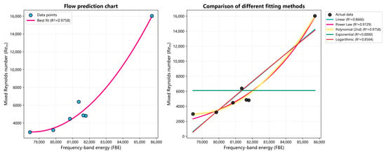
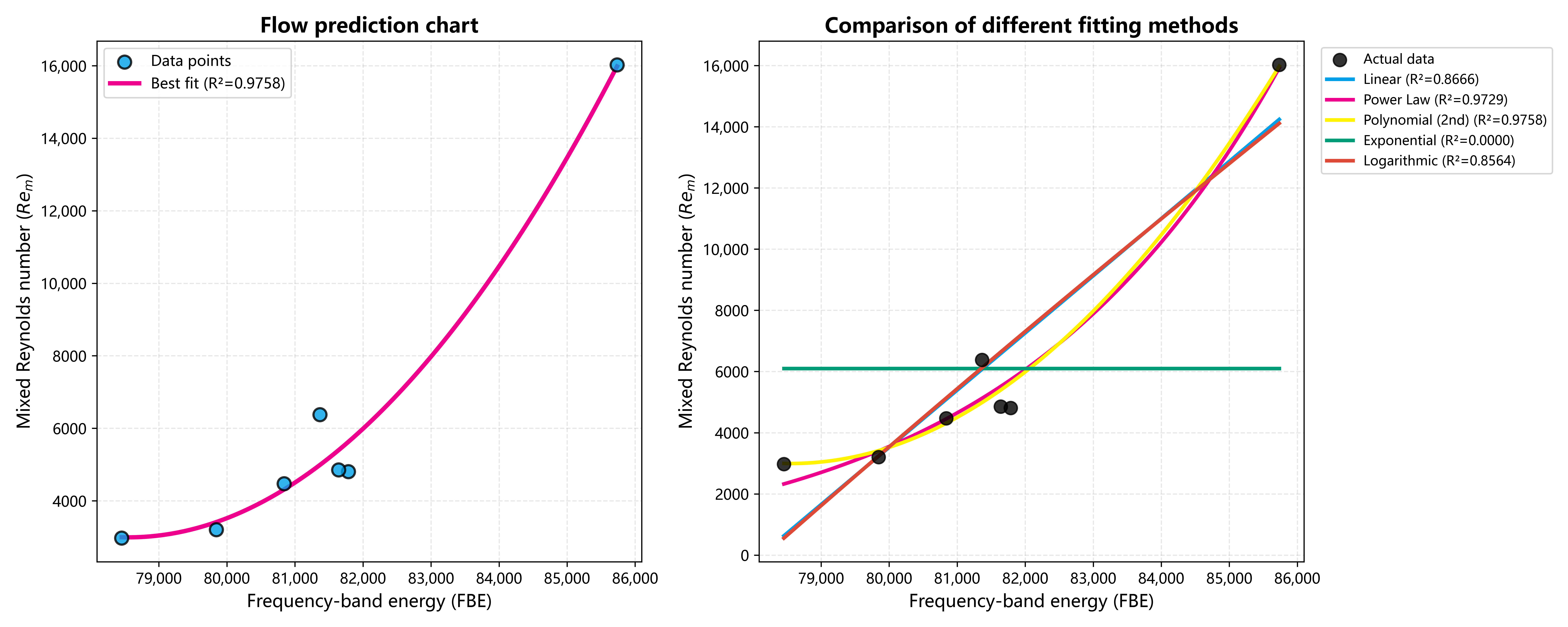
Based on the discussion above, the core principle for defining the Reynolds number is that it should reflect the phase characteristics that dominate wall shear and turbulent kinetic energy generation. In bubbly flow, because the two phases are well mixed, the mixture Reynolds number can reasonably describe the overall flow state. However, in stratified flow, wavy flow, and slug flow, the water phase consistently controls the wall-shear process. The use of a mixture Reynolds number would introduce unreasonable property weighting and lead to systematic underestimation of the actual shear intensity. Therefore, the water-phase Reynolds number was adopted. Although water cut does not directly enter the Reynolds number calculation under stratified-flow, wavy-flow, and slug-flow conditions, it has an important effect on the DAS frequency-band energy distribution through structural parameters such as interfacial-wave characteristics, gas-slug length, and slug-passage frequency. This effect is mainly reflected in the degree of dispersion of DAS energy under the same Reynolds number. After characteristic Reynolds numbers were selected according to flow regime, the correspondence between DAS frequency-band energy and Reynolds number under different flow regimes retained physical consistency. This provides a reliable basis for the subsequent construction of flow-regime-specific frequency-band energy–Reynolds number prediction models. On this basis, the Reynolds numbers under different well inclinations and operating conditions were calculated in this study. A Reynolds-number regression chart was then constructed together with frequency-band energy, as shown in Figure 6.

Figure 6. Regression chart of Reynolds numbers. (left) Best-fit curve. (right) Curves obtained using different fitting methods.

Taking the case of a well inclination of 90° and a water cut of 10% as an example, the horizontal axis represents frequency-band energy, and the vertical axis represents the Reynolds number. Linear, exponential, and quadratic fits were compared. The coefficient of determination, R², indicated that the quadratic function provided the best fit. A quadratic relationship between FBE and the Reynolds number was obtained for each calibrated condition:

Re = α · FBE² + β · FBE + γ

(15)

Following the above processing, the discrete relationships between the Reynolds number and frequency-band energy under different experimental conditions were represented uniformly by quadratic functions. The fitted coefficients were then associated with the corresponding operating parameters, such as well inclination angle and water cut, to construct a database of quadratic-function coefficients (Table 2).

Table 2. Database of quadratic-function coefficients.

Well Inclination (o)	Water Cut (%)	α (×10−4)	β	γ
90	0	−1.44	35.557	−1,854,138.56
90	10	17.2	−268.208	10,507,210.279
90	30	2.45	−36.339	1,373,504.692
90	50	2.88	−42.606	1,581,889.600
90	90	12.3895	−191.214	7,388,131.408
90	100	−0.475	10.528	−526,322.312
88	1	−0.981	17.560	−754,529.091
88	10	7.92	−121.962	4,691,677.331
88	30	1.62	−23.676	874,154.543
88	50	0.241	−2.098	30,585.237
88	70	−4.92	87.305	−3,747,373.665
88	90	−9.68	160.416	−6,606,392.171
85	1	1.60	−20.052	606,898.893
85	10	1.52	−22.814	861,020.088
85	30	1.90	−24.578	791,776.046
85	50	1.78	−25.524	920,676.334
85	70	5.96	−79.036	2,564,987.325
85	90	0.055	3.367	−266,495.546

This database not only preserves the relationships between the Reynolds number and frequency-band energy under different operating conditions but also transforms the raw experimental data into standardized training samples suitable for model development. However, the function coefficients stored in the database correspond only to the discrete operating conditions covered by the experimental calibration, whereas the target well inclination angles and water cuts encountered in practical applications may not exactly match the calibrated conditions. Therefore, based on this database, a predictive model was developed using the operating-condition parameters as inputs and the quadratic-function coefficients as outputs. The function coefficients predicted for the target operating condition are combined with the DAS frequency-band energy measured under that condition using the same experimental apparatus and measurement configuration to determine the characteristic Reynolds number, total flow rate, and individual phase flow rates. This procedure enables the transition from discrete experimental calibration to flow-rate prediction under the target operating condition.

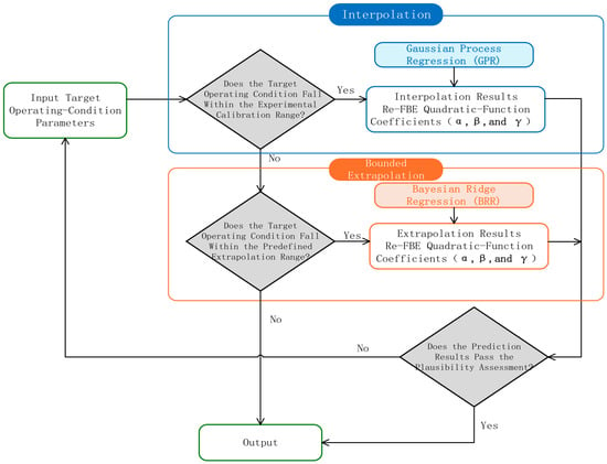
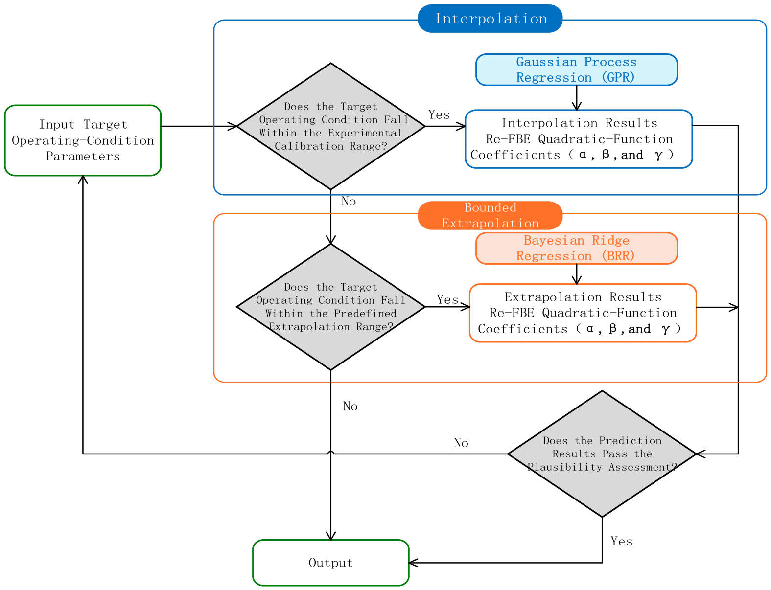
To balance the interpolation accuracy within the calibrated parameter range and the stability of bounded extrapolation near the parameter boundaries, a domain-partitioned prediction strategy combining Gaussian process regression (GPR) and Bayesian ridge regression (BRR) was adopted, as shown in the Figure 7.

Figure 7. Prediction workflow.

Separate prediction models were developed for each well inclination angle. Water cut, expressed as a percentage, was used as the input variable, and the fitted coefficients α, β, and γ of the quadratic Re–FBE relationship at the calibrated operating conditions were used as the output variables. When the target water cut falls within the calibration range for the corresponding well inclination, GPR is used to interpolate each of the three function coefficients independently, using the product of a constant kernel and a radial basis function (RBF) kernel:

$$k\left(x,x^{\prime }\right)=\mathit{Cexp}\left[-{\displaystyle \frac{{\left(x-x^{\prime }\right)}^2}{2{\mathcal{l}}^2}}\right]$$

(16)

Here, x denotes water cut expressed as a percentage, C is the kernel amplitude, and 𝓁 is the length scale. The initial values of the kernel amplitude and length scale were set to 1 and 10, respectively, with both constrained to the range [10⁻⁵,10⁵] during optimization. Their values were determined by maximizing the log marginal likelihood using the L-BFGS-B algorithm, without additional optimization restarts. Each output coefficient was standardized before fitting, and the predictions were transformed back to the original scale. No explicit probability priors were assigned to the length scale or noise variance. Instead, a fixed regularization term of 10⁻¹⁰ was added to the diagonal of the training kernel matrix after output standardization.

In the limited-extrapolation branch, BRR is used to predict the corresponding coefficients when the target water cut falls outside the calibration range. A linear model with an intercept is employed to predict each function coefficient separately:

y = b₀ + ωx + ε, ε~$𝒩$(0,τ⁻¹)

(17)

Here, y represents α, β, or γ in the respective regression models, b₀ is the intercept, and ω is the regression weight. Compared with unconstrained nonlinear extrapolation, using this linear model to describe the trend of each function coefficient with water cut can reduce the risk of coefficient fluctuations or numerical divergence under small-sample conditions. A zero-mean Gaussian prior is assigned to the regression weight:

ω|λ~$𝒩$(0,λ⁻¹)

(18)

Weakly informative Gamma hyperpriors are assigned to the regression-weight precision and noise precision [26,27]:

τ, λ~Gamma(10⁻⁶,10⁻⁶)

(19)

The Gamma distributions use a shape–rate parameterization. The shape and rate parameters of the hyperpriors for both the noise precision and weight precision are set to 10⁻⁶ to regularize parameter estimation. The posterior mean of each function coefficient is used as a deterministic point prediction to reconstruct the Re–FBE relationship for the target operating condition. To reduce the risk of physically implausible extrapolation, the reconstructed function is applied only within the experimentally determined valid FBE range. Bayesian ridge regression is restricted to the experimentally validated limited-extrapolation region adjacent to the calibrated water-cut boundary for the corresponding well inclination. The model does not currently provide flow-rate predictions for water cuts substantially beyond the experimental coverage, unvalidated water-cut conditions, or well inclinations for which no corresponding database has been established.

In summary, the domain-partitioned strategy uses the coefficient trends in the calibration data to reconstruct Re–FBE relationships for target water cuts within the calibration range and its validated vicinity, supporting flow-rate prediction under limited experimental coverage.

3.4. Module Design

The flow-rate prediction procedure was implemented in reusable software modules.

As illustrated in Figure 8, software modules were developed to implement the proposed flow-rate prediction procedure, incorporating data acquisition, preprocessing, frequency-band energy calculation, flow-rate prediction, and result visualization. The software reads and preprocesses the DAS data, extracts FBE, calculates flow rate using the coefficient-prediction model, and displays the prediction results.

Figure 8. Workflow of the main modules.

3.5. Validation of the Prediction Model

The flow-rate prediction model developed above and its associated software modules were validated using experimental data obtained under high-gas-rate, low-water-cut conditions. The validation data were independent of those used to establish the regression charts and train the coefficient-prediction models, with no overlap between the datasets. Water cuts in the target Fuling gas-well applications are generally below 10%, but the calibration database covers only selected conditions. The model was therefore used to reconstruct Re–FBE relationships for selected water cuts below 10%. The predicted quadratic coefficients are listed in Table 3.

Table 3. Predicted quadratic-function coefficients.

Water Cut (%)	Well Inclination (o)	α′ (×10−4)	β′	γ′
0.5	90	2.718	−37.314	1,281,119.785
0.75	90	4.003	−59.076	2,184,551.960
1	90	5.070	−77.723	2,983,748.358
1.5	90	7.487	−114.123	4,353,646.016
2	90	9.296	−142.974	5,502,414.490
3	90	12.103	−188.087	7,312,179.103
4	90	14.137	−220.781	8,624,368.421
0.45	88	1.268	−17.873	635,091.036
0.75	88	0.354	−3.474	70,396.718
0.5	88	1.307	−18.476	658,721.813
0.68	88	0.804	−10.566	348,497.253
1.5	88	1.430	−20.499	738,096.800
2	88	1.563	−22.523	817,461.567
3	88	1.563	−22.523	817,465.786
4	88	1.564	−22.523	817,471.786
0.45	85	1.682	−20.641	606,898.892
0.5	85	1.669	−20.542	606,898.893
0.68	85	1.635	−20.283	606,898.893
0.75	85	1.626	−20.213	606,898.893
0.9	85	1.611	−20.103	606,898.893
1.5	85	1.590	−19.939	606,898.893
2	85	1.587	−19.921	606,898.893
3	85	1.587	−19.916	606,898.893
4	85	1.577	−19.841	606,898.893

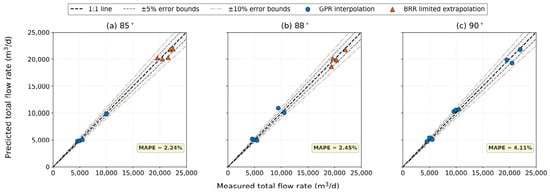
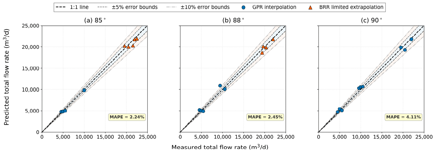
Based on the prediction results obtained from the above regression charts, the frequency-band energy values measured under high-gas-rate and low-water-cut conditions were matched with their corresponding Reynolds numbers. The flow rate under each operating condition was then calculated using Equation (6). Finally, the experimental reference flow rates were compared with the predictions, as shown in Figure 9.

Figure 9. Comparison of experimental references and predicted total flow rates.

Figure 9 visually illustrates the agreement between the measured and predicted total flow rates at different well inclination angles. Overall, both the GPR interpolation results and the BRR bounded-extrapolation results are distributed near the 1:1 line, indicating that the domain-partitioned prediction model captures the variation in total flow rate reasonably well. To quantify model performance under different operating conditions, the measured total flow rates, water cuts, predicted flow rates, and corresponding errors are summarized in Table 4.

Table 4. Prediction results and errors.

Total Flow Rate (m3/d)	Well Inclination (o)	Water Cut (%)	Predicted Total Flow Rate (m3/d)	Prediction Branch	Relative Error (%)
50 00	85	2	4783.7	GPR interpolation	4.32
5000	85	3	4830.8	GPR interpolation	3.38
5000	85	4	5006.7	GPR interpolation	0.13
10,000	85	1.5	9809.4	GPR interpolation	1.9
20,000	85	0.5	20,234	BRR extrapolation	1.17
20,000	85	0.75	20,009.9	BRR extrapolation	0.05
22,000	85	0.45	20,297	BRR extrapolation	7.74
22,000	85	0.68	21,760.8	BRR extrapolation	1.08
22,000	85	0.9	21,921	BRR extrapolation	0.35
5000	88	2	5189.5	GPR interpolation	3.78
5000	88	3	5023.3	GPR interpolation	0.46
5000	88	4	4893.4	GPR interpolation	2.13
10,000	88	2	10,884	GPR interpolation	8.84
10,000	88	1.5	10,084.6	GPR interpolation	0.84
22,000	88	0.45	21,783.5	BRR extrapolation	0.98
20,000	88	0.75	20,099	BRR extrapolation	0.49
20,000	88	0.5	19,868.8	BRR extrapolation	0.65
19,382	88	0.68	18,632	BRR extrapolation	3.86
5000	90	2	4737.2	GPR interpolation	5.25
5000	90	3	5449	GPR interpolation	8.98
5000	90	4	5109.1	GPR interpolation	2.18
10,000	90	2	10,295.1	GPR interpolation	2.95
10,000	90	1.5	10,572.1	GPR interpolation	5.72
10,000	90	1	10,643.4	GPR interpolation	6.43
20,000	90	0.75	19,861.9	GPR interpolation	0.69
20,000	90	0.5	19,241.9	GPR interpolation	3.79
22,000	90	0.45	21,783.5	GPR interpolation	0.98

The flow-rate predictions were evaluated using 26 independent operating conditions, comprising 17 GPR interpolation cases and nine BRR extrapolation cases. Overall, the model achieved an RMSE of 492.55 m³/d, an MAE of 329.24 m³/d, and a MAPE of 3.01%, with a maximum absolute relative error of 8.98%. Of the 26 validation cases, 20 had absolute relative errors no greater than 5%, accounting for 76.92% of the total, and all predictions were within 10%. These results indicate that the domain-partitioned prediction model provides good flow-rate prediction accuracy within the validated experimental range.

For the GPR interpolation branch, 17 validation cases yielded an RMSE of 395.04 m³/d, an MAE of 299.91 m³/d, and a MAPE of 3.64%, with a maximum absolute relative error of 8.98%. Twelve predictions had absolute relative errors no greater than 5%, accounting for 70.59% of the cases. For the BRR extrapolation branch, nine validation cases yielded an RMSE of 637.26 m³/d, an MAE of 384.64 m³/d, and a MAPE of 1.82%, with a maximum absolute relative error of 7.74%. Eight predictions had absolute relative errors no greater than 5%, accounting for 88.89% of the cases, and all predictions were within 10%. The BRR extrapolation branch yielded a lower MAPE than the GPR interpolation branch, but its RMSE and MAE were relatively higher. The BRR extrapolation branch yielded a lower MAPE but higher RMSE and MAE than the GPR interpolation branch. This reflects the different numbers of validation cases, flow-rate ranges, and error distributions in the two branches. Overall, the results indicate that the proposed model achieved good prediction performance under high-gas-rate, low-water-cut conditions.

However, prediction errors remained under some high-flow-rate conditions. These errors may reflect the combined effects of complex influences on the DAS response at high flow rates, limited instrumental accuracy, and deviations in the imposed phase flow-rate ratios. In addition, flow regimes were classified by visual inspection of experimental videos during model development, introducing potential classification uncertainty under transitional conditions. Because different flow-regime classifications correspond to different definitions of the characteristic Reynolds number, misclassification may alter the Re values of the calibration data and the fitted Re–FBE relationships, thereby affecting subsequent coefficient prediction and flow-rate calculation. At very low water cuts, input errors may have a greater influence on flow-rate predictions. For conditions characterized by a Reynolds number based on water superficial velocity, the total flow rate is inversely proportional to water cut when the predicted Reynolds number, fluid properties, and pipe diameter are held constant. The first-order relative variation satisfies:

δQ/Q ≈ −δC_w/C_w

(20)

Therefore, the same absolute deviation in water cut produces a larger relative change in flow rate at lower water cuts. Addressing this sensitivity will be a key focus of subsequent model refinement and optimization.

3.6. Comparison with the Cross-Correlation Method

To further assess prediction reliability, the cross-correlation method was applied to the same test data, and its flow-rate estimates were compared with those of the proposed model. In this experiment, due to the presence of multi-modal disturbances, interfacial waves, and vortex structures [28] in gas–water two-phase flow, the propagation direction and velocity of the disturbances along the optical fiber are no longer unique. Therefore, the conventional upflow–downflow velocity method cannot be used for flow rate calculation in this experiment [10].

The cross-correlation method was used to estimate flow rate based on the characteristics of horizontal gas–water flow [29]. It estimates disturbance propagation velocity from the time delay between signals recorded at different measurement locations along the optical fiber [7]. Signals from selected measurement locations were cross-correlated to determine the propagation delay, Δt. The velocity, v, was then calculated from the measurement-point spacing, Δx, using the following expression:

$$v={\displaystyle \frac{\Delta x}{\Delta t}}.$$

(21)

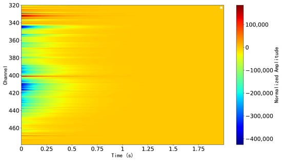
DAS velocity-tracking approaches based on coherent spatiotemporal propagation patterns have previously been used for flow monitoring and production profiling [30]. During the experiment, since DAS can continuously record the vibration responses along the wellbore, adjacent measurement points usually exhibit similar disturbance characteristics with a certain time delay. This is often manifested in the space–time propagation map (Figure 10) as inclined streaks or “plume” structures with a certain inclination angle, which essentially reflect the spatial propagation process of disturbances [8,31].

Figure 10. Space–time propagation map.

The results calculated using the cross-correlation method for the test data under three well inclination angles are shown in Table 5.

Table 5. Calculation results and errors.

Total Flow Rate (m3/d)	Well Inclination (o)	Water Cut (%)	Gas Phase (m3/d)	Water Phase (m3/d)	Predicted Total Flow Rate (m3/d)	Predicted Gas Phase (m3/d)	Predicted Water Phase (m3/d)	Relative Error (%)
5000	85	2	4900	100	5702.4	5588.352	114.048	14.05
5000	85	3	4850	150	5529.6	5363.712	165.888	10.59
5000	85	4	4800	200	4924.8	4727.808	196.992	1.50
10,000	85	1.5	9850	150	9849.6	9701.856	147.744	1.50
20,000	85	0.5	19,900	100	16,675.2	16,591.824	83.376	16.62
20,000	85	0.75	19,850	150	15,638.4	15,521.112	117.288	21.81
22,000	85	0.45	21,901	99	24,710.4	24,599.203	111.1968	12.32
22,000	85	0.68	21,850.4	149.6	25,315.2	25,143.057	172.14336	15.07
22,000	85	0.9	21,802	198	16,934.4	16,781.99	152.4096	23.03
5000	88	2	4900	100	6877.4	6739.852	137.548	37.55
5000	88	3	4850	150	6912	6704.64	207.36	38.24
5000	88	4	4800	200	6220.8	5971.968	248.832	24.42
10,000	88	2	9800	200	10,108.8	9906.624	202.176	1.09
10,000	88	1.5	9850	150	10,281.6	10,127.376	154.224	2.82
22,000	88	0.45	21,901	99	24,796.8	24,685.214	111.5856	12.71
20,000	88	0.75	19,850	150	12,096	12,005.28	90.72	39.52
20,000	88	0.5	19,900	100	14,774.4	14,700.528	73.872	26.13
19,382	88	0.68	19,250	132	14,688	14,588.122	99.8784	24.22
5000	90	2	4900	100	5184	5080.32	103.68	3.68
5000	90	3	4850	150	3628	3519.16	108.84	27.44
5000	90	4	4800	200	6048	5806.08	241.92	20.96
10,000	90	2	9800	200	10,368	10,160.64	207.36	3.68
10,000	90	1.5	9850	150	12,096	11,914.56	181.44	20.96
10,000	90	1	9900	100	10,108.8	10,007.712	101.088	1.09
20,000	90	0.75	19,850	150	10,454.4	10,375.992	78.408	47.73
20,000	90	0.5	19,900	100	14,688	14,614.56	73.44	26.56

As shown in Table 4 and Table 5, the error statistics indicate that the conventional cross-correlation method yielded a mean absolute percentage error (MAPE) of 18.28%, with a root-mean-square error (RMSE) and mean absolute error (MAE) of 3563.52 and 2549.64 m³/d, respectively. Its maximum absolute relative error reached 47.73%. In comparison, the prediction model proposed in this study achieved a MAPE of 3.01%, while the RMSE and MAE decreased to 492.55 and 329.24 m³/d, respectively, and the maximum absolute relative error was 8.98%. Relative to the conventional cross-correlation method, the proposed model reduced the MAPE, RMSE, and MAE by 83.54%, 86.18%, and 87.09%, respectively, while reducing the maximum absolute relative error by 81.19%.

Regarding the error distribution, the proposed model exhibited a lower absolute relative error than the conventional cross-correlation method under 22 evaluated operating conditions, accounting for 84.62% of all comparative cases. For the proposed model, 20 prediction points fell within the ±5% error range, accounting for 76.92%, and all prediction points were within the ±10% error range. In contrast, only seven results obtained using the conventional cross-correlation method fell within the ±5% error range, accounting for 26.92%, while the relative errors under all remaining operating conditions exceeded 10%. Further analysis by well inclination angle showed that the MAPE values of the proposed model at 85°, 88°, and 90° were 2.24%, 2.45%, and 4.50%, respectively, compared with 12.94%, 22.97%, and 19.01% for the conventional cross-correlation method. These results demonstrate that the proposed domain-partitioned prediction model more effectively captures the response relationship between DAS frequency-band energy and flow rate under different well inclination angles and water cuts, exhibiting substantially greater prediction accuracy and adaptability to varying operating conditions than the conventional cross-correlation method. The error analysis indicates that the two methods follow different computational pathways and therefore have different potential sources of error. The cross-correlation method first estimates the propagation delay of trackable disturbances between measurement locations and then converts the resulting propagation velocity into flow rate. Its estimates may be affected by uncertainty in correlation-peak identification, the evolution of flow structures between measurement locations, and differences between the characteristic propagation velocity and the mean velocity used for flow-rate calculation. The proposed method predicts flow rate using experimentally calibrated Re–FBE relationships and predicted functional coefficients. In addition to the instrumental errors discussed above, its errors may arise from frequency-band energy measurement, empirical-relationship fitting, coefficient prediction, and flow-regime identification.

4. Conclusions and Recommendations

(1) DAS was used to investigate acoustic responses to near-horizontal gas–water two-phase flow in a large-diameter flow-loop facility under different flow-rate and water-cut conditions in the study. The measured signal energy was concentrated primarily below 500 Hz, and the frequency-band energy reached its highest level near a water cut of 50% among the investigated conditions.

(2) Based on the strong correlation between the Reynolds number and frequency-band energy, a flow-rate prediction model was constructed, and the model coefficients corresponding to different water cuts were determined. In practical application, the water cut measured at the wellhead can be used as a constraint, and the frequency-band energy can be calculated from the DAS signal. The Reynolds number, superficial velocity, total flow rate, and individual phase flow rates can then be estimated, completing the calculation workflow.

(3) Future research can further expand the experimental conditions by adding data from high-temperature and high-pressure conditions, ultra-high-flow-rate conditions, and ultra-low-water-cut conditions. The experimental setup can also be improved, for example, by adding a temperature-control system and optimizing the fiber layout. A multidimensional parameter-correlation model can then be established. In addition, DAS can be combined with DTS, array probes, and other instruments to identify production locations, fluid types, and flow regimes qualitatively or quantitatively. This would improve the accuracy of the model in production-profile interpretation and further enhance the practicality and reliability of this technology for oil and gas field development monitoring.

(4) The proposed model was developed and validated using air–water experiments near room temperature and at atmospheric pressure; its applicability is therefore limited to the tested conditions. In actual gas wells, high temperatures, high pressures, and different fluid compositions may alter fluid properties, phase slip, flow regimes, and the DAS response. Wellbore configuration, fiber installation and coupling, background noise, and uncertainties in water cut and flow-regime identification may further affect prediction accuracy. Although Reynolds-number-based calculations explicitly account for density, viscosity, and pipe diameter, field application requires site-specific fluid properties, assessment of the DAS response, and validation and, where necessary, recalibration under representative operating conditions.

References

- Malik, A.; Pao, W.; Mohamad, H. Distributed Acoustic Sensing (DAS) in Multiphase Flow Monitoring: A Systematic Review. Flow Meas. Instrum. 2026, 109, 103238. [Google Scholar] [CrossRef] [Scilit]
- Yu, X.; Yang, D. Application progress of DAS in horizontal-well fracturing and monitoring. Inn. Mong. Petrochem. Ind. 2025, 51, 31–35. (In Chinese) [Google Scholar]
- He, H. Application of distributed fiber-optic DAS logging technology in offset-well fracturing monitoring for shale gas horizontal well. J. Jianghan Pet. Univ. Staff. Work. 2025, 38, 15–18. (In Chinese) [Google Scholar] [CrossRef]
- in’t Panhuis, P.; den Boer, H.; van der Horst, J.; Paleja, R.; Randell, D.; Joinson, D.; McIvor, P.; Green, K.; Bartlett, R. Flow Monitoring and Production Profiling Using DAS. Presented at the SPE Annual Technical Conference and Exhibition, Amsterdam, The Netherlands, 27–29 October 2014. SPE-170917-MS. [Google Scholar] [CrossRef] [Scilit]
- Zett, A.; Webster, M.; Ragbirsingh, F.; Gysen, A.; Limkar, P.; Johnson, J. A case study of optical sensing applicability in reservoir surveillance: The non-unique solution dilemma. In SPWLA Annual Logging Symposium (SPWLA-2014-P); SPWLA: Houston, TX, USA, 2014. [Google Scholar]
- Karrenbach, M.; Ridge, A.; Cole, S.; Boone, K.; Kahn, D.; Rich, J.; Sliver, K.; Langton, D. DAS microseismic monitoring and integration with strain measurements in hydraulic fracture profiling. In Proceedings of the SPE/AAPG/SEG Unconventional Resources Technology Conference, URTeC 2017, Austin, TX, USA, 24–26 July 2017. URTEC-2670716. [Google Scholar] [CrossRef] [Scilit]
- Jin, G.; Friehauf, K.; Roy, B.; Constantine, J.J.; Swan, H.W.; Krueger, K.R.; Raterman, K.T. Fiber optic sensing-based production logging methods for low-rate oil producers. In Proceedings of the SPE/AAPG/SEG Unconventional Resources Technology Conference, URTEC, Denver, CO, USA, 22–24 July 2019. D013S019R005. [Google Scholar] [CrossRef] [Scilit]
- Titov, A.; Fan, Y.; Jin, G.; Tura, A.; Kutun, K.; Miskimins, J. Experimental investigation of distributed acoustic fiber-optic sensing in production logging: Thermal slug tracking and multiphase flow characterization. In SPE Annual Technical Conference and Exhibition; D041S044R006; SPE: Richardson, TX, USA, 2020. [Google Scholar] [CrossRef] [Scilit]
- Tabjula, J.; Shetty, R.; Adeyemi, T.; Sharma, J. Empirical Correlations for Predicting Flow Rates Using Distributed Acoustic Sensor Measurements, Validated with Wellbore and Flow Loop Data Sets. SPE Prod. Oper. 2023, 38, 678–693. [Google Scholar] [CrossRef] [Scilit]
- Ali, S.; Jin, G.; Fan, Y. Characterization of gas–liquid two-phase slug flow using distributed acoustic sensing in horizontal pipes. Sensors 2024, 24, 3402. [Google Scholar] [CrossRef] [Scilit]
- Zeng, T.; Li, L.; Ren, C.; Li, Z.; Liu, J. Laboratory experiment and application of gas-well production performance monitoring based on distributed acoustic sensing technology. J. China Univ. Pet. (Ed. Nat. Sci.) 2025, 50, 128–135. (In Chinese). Available online: https://link.cnki.net/urlid/37.1441.TE.20250714.1420.002 (accessed on 24 May 2025).
- Luo, H.; Ran, F.; Li, H.; Wang, W.; Zuo, K.; Yang, W.; Zhang, X.; Li, Y. Experimental study on acoustic response laws of gas-water two-phase flow in horizontal wells. Nat. Gas Geosci. 2026, 37, 391–402. (In Chinese) [Google Scholar]
- Wang, Y.; Xu, Z.; Tian, Z.; Liu, W.; Yang, J.; Huang, Q. Progress in the flocculation and sedimentation mechanisms and jet mixing transportation of heavy components in crude oil storage tanks. J. Pipeline Sci. Eng. 2026; in press. [CrossRef] [Scilit]
- Wang, Y.; Peters, B.; Yin, R.; Pu, X.; Liu, W.; Qin, Y.; Zhang, Y.; Huang, Q. Investigation of deposition behavior in non-Newtonian oil-wax slurry pipeline transport based on experiment and CFD-CGDEM method. Results Eng. 2025, 27, 105922. [Google Scholar] [CrossRef] [Scilit]
- Yin, Y.; Zheng, H.; Li, A.; Tian, G.; Song, M. Flow characteristics and low-resistance optimization of S-elbows in heating pipelines based on secondary flow and energy dissipation. Appl. Therm. Eng. 2026, 300, 131579. [Google Scholar] [CrossRef] [Scilit]
- Wang, W.; Gao, S.; Wu, H.; Chen, P.; Xu, D.; Xu, H.; Jing, M.; Sun, Q.; Chang, S.; Sun, Z.; et al. Reverse Tesla valve modulated efficient water evaporation and cooling. Nat. Commun. 2026, 17, 8100. [Google Scholar] [CrossRef] [Scilit]
- Zarastvand, M.R.; Goodarzvand Chegini, S.; Talebitooti, R. Novel hybrid-stiffened cylindrical metastructures for broadband sound insulation. Int. J. Mech. Sci. 2026, 326, 111866. [Google Scholar] [CrossRef] [Scilit]
- Godin, O.A. Sensitivity of distributed acoustic sensing to waves in fluids. Phys. Fluids 2026, 38, 016123. [Google Scholar] [CrossRef] [Scilit]
- Wang, Y.; Yu, Y.; Liu, Z.; Chang, Y.; Zhao, X.; Wang, Q. Experimental study on gas-liquid two-phase stratified flow at high pressure in a horizontal pipe. Energies 2024, 17, 1056. [Google Scholar] [CrossRef] [Scilit]
- Wallis, G.B. One-Dimensional Two-Phase Flow; Courier Dover Publications: Garden City, NY, USA, 2020. [Google Scholar]
- Bouderbal, A.; Salhi, Y.; Arabi, A.; Si-Ahmed, E.K.; Legrand, J.; Arhaliass, A. Experimental investigation of different sub-regimes in horizontal stratified and intermittent gas-liquid two-phase flow: Flow map and analysis of pressure drop fluctuations. Chem. Eng. Res. Des. 2024, 210, 407–424. [Google Scholar] [CrossRef] [Scilit]
- Arabi, A.; Zenati, Y.; Legrand, J.; Si-Ahmed, E.K. Sub-regimes of horizontal gas–liquid intermittent flow: State-of-the-art and future challenges. Exp. Therm. Fluid Sci. 2025, 160, 111281. [Google Scholar] [CrossRef] [Scilit]
- Yang, E. Study on Gas-Water Two-Phase Flow Laws and Characteristic Parameter Characterization Methods in Horizontal Wells. Ph.D. Thesis, Southwest Petroleum University, Nanchong, China, 2023. (In Chinese) [Google Scholar] [CrossRef]
- Colombo, M.; Fairweather, M. Prediction of bubbly flow and flow regime development in a horizontal air-water pipe flow with a morphology-adaptive multifluid CFD model. Int. J. Multiph. Flow 2025, 184, 105112. [Google Scholar] [CrossRef] [Scilit]
- Shakarami, R.; Sadeghi, M.T. Gas-liquid two-phase flow measurement based on emitted acoustic signal anomaly and deep learning approach. Flow Meas. Instrum. 2025, 107, 103097. [Google Scholar] [CrossRef] [Scilit]
- Xu, M.; Lan, S.; Kang, L. Bayesian Bridge Gaussian Process Regression. arXiv 2025, arXiv:2511.17415. [Google Scholar] [CrossRef] [Scilit]
- Michael Kielstra, P.; Lindsey, M. A gradient-based and determinant-free framework for fully Bayesian Gaussian process regression. SIAM/ASA J. Uncertain. Quantif. 2025, 13, 1709–1734. [Google Scholar] [CrossRef] [Scilit]
- Khan, U.; Pao, W.; Sallih, N. A review: Factors affecting internal two-phase flow-induced vibrations. Appl. Sci. 2022, 12, 8406. [Google Scholar] [CrossRef] [Scilit]
- Ashraf, A.; Masoudi, A.; Vahdati, N.; Brambilla, G. A Noninvasive Solution for Multiphase Flow Analysis in Pipelines Based on High-Resolution Distributed Acoustic Sensing (HR-DAS). Arab. J. Sci. Eng. 2026, 51, 21681–21700. [Google Scholar] [CrossRef] [Scilit]
- Paleja, R.; Mustafina, D.; in’t Panhuis, P.; Park, T.; Randell, D.; van der Horst, J.; Crickmore, R. Velocity Tracking for Flow Monitoring and Production Profiling Using Distributed Acoustic Sensing. Presented at the SPE Annual Technical Conference and Exhibition, Houston, TX, USA, 28–30 September 2015. SPE-174823-MS. [Google Scholar] [CrossRef] [Scilit]
- Seo, H.; Mensah, E.; Almeida, C.M.D.; Amudzi-Deku, A.; Leggett, S. Monitoring Liquid Slugs Using Distributed Acoustic Sensing and an Air Gun. Sensors 2026, 26, 1278. [Google Scholar] [CrossRef] [Scilit]
Disclaimer/Publisher’s Note: The statements, opinions and data contained in all publications are solely those of the individual author(s) and contributor(s) and not of MDPI and/or the editor(s). MDPI and/or the editor(s) disclaim responsibility for any injury to people or property resulting from any ideas, methods, instructions or products referred to in the content. |
© 2026 by the authors. Licensee MDPI, Basel, Switzerland. This article is an open access article distributed under the terms and conditions of the Creative Commons Attribution (CC BY) license.