Reduced-Dimension Profile Inversion for Material Balance Analysis of Water-Drive Gas Reservoirs

Abstract

Trade-offs between gas expansion and delayed aquifer support complicate the joint estimation of original gas in place (OGIP) and aquifer response parameters in water-drive gas reservoirs. Here, we combine response time parameterization and analytical aquifer-state propagation under piecewise linear pressure histories with the established variable-projection principle. The OGIP and aquifer capacitance are estimated using bounded conditional linear least squares, leaving a one-dimensional nonlinear search over the response time. Synthetic tests are used to recover prescribed parameters and characterize sensitivity to pressure errors and sampling density, while approximate 95% profile likelihood confidence intervals quantify parameter uncertainty under a specified withdrawal error model. In the synthetic pressure-thinning test, retaining 60% of the noninitial pressure observations gives a response time error of −2.06% when the OGIP and aquifer capacitance are fixed. Applied to approximately 20 years of field history, the method yields an OGIP estimate 0.67% above the operator-provided reference value and a normalized root mean square error of 0.009375. The field profiles reveal compensating parameter adjustments and branches governed by active bounds. The formulation supports joint evaluation of gas volume and aquifer dynamics while making parameter compensation and the role of physical constraints explicit.

1. Introduction

Material balance analysis remains one of the most widely used reservoir-scale methods for estimating original gas in place (OGIP) because it links the average reservoir pressure, cumulative production, and fluid properties through conservation of mass [1]. Its interpretation is relatively straightforward for volumetric gas reservoirs, where pressure depletion is governed primarily by gas expansion. The situation becomes considerably more complicated when the reservoir is supported by a communicating aquifer. Water influx replaces part of the withdrawn reservoir volume, moderates pressure decline, and changes the relationship between pressure and cumulative gas production [2]. Consequently, conventional p/z-based extrapolation can substantially overestimate OGIP when aquifer support is ignored [3,4]. More importantly, aquifer support does not necessarily produce an obvious curvature in the observed p/z trend. Under certain combinations of aquifer response and production history, a water-drive gas reservoir may still exhibit an approximately linear p/z relationship, and therefore, appear volumetric over the available observation period [5]. Reliable reserve estimation in such systems therefore requires more than fitting a depletion trend; the contribution of time-dependent water influx must be separated from gas expansion within the material balance framework.

A large body of work has been devoted to describing aquifer contribution in material balance analysis. The transient solutions of van Everdingen and Hurst established a rigorous basis for representing pressure propagation and water influx under time-dependent boundary conditions [6], while Carter and Tracy reformulated transient water-influx calculations into a convenient time-step procedure for reservoir engineering applications [7]. Fetkovich subsequently introduced a finite-aquifer formulation in which water influx is governed jointly by the pressure difference between an aquifer and reservoir and by depletion of the aquifer itself [8]. Analytical extensions have further incorporated finite bottom-water support into material balance analysis [9]. Although these formulations differ in geometry and flow assumptions, they share an important implication: cumulative water influx is not determined by the current reservoir pressure alone but also depends on the preceding pressure history and the evolving aquifer state. Retaining this dynamic response is therefore essential when long-term pressure measurements are available and aquifer support significantly affects reservoir performance evaluation.

Once aquifer behavior is introduced into material balance, reservoir evaluation becomes an inverse problem rather than a simple depletion extrapolation problem. The OGIP, aquifer storage capacity, and aquifer deliverability may compensate for one another during history matching, while uncertainties in pressure and fluid properties further influence the inferred parameter set. Early studies recognized these difficulties. McEwen investigated water-drive material balance calculations under pressure uncertainty and introduced independently estimated physical information to reduce the number of regression unknowns [10]. Chierici et al. demonstrated that different reservoir–aquifer combinations may reproduce similar historical pressure–production responses, indicating that reservoir parameters cannot always be uniquely identified from production history alone [11]. Sills combined aquifer and reservoir expansion terms to estimate hydrocarbon volumes via linear regression at specified aquifer parameters and examined the associated regression errors and physical consistency of the inferred aquifer description [12]. Vega and Wattenbarger optimized aquifer influence functions for trial OGIP values and interpreted the resulting error curves to estimate OGIP and aquifer performance [13]. Yildiz combined McEwen and apparent-gas-in-place diagnostics with modified Roach and Havlena–Odeh plots, where applicable, to narrow the range of possible estimates [14]. Pressure and pressure–volume–temperature (PVT) uncertainties introduce further variability into material balance estimation [15]. These studies indicate that a small history-matching residual does not necessarily imply that all estimated parameters are physically well constrained. Therefore, an effective inversion framework should provide not only parameter estimates but also information regarding parameter trade-offs and practical identifiability.

Recent studies have further extended water-drive material balance analysis through production diagnostics and dynamic formulations [16,17,18]. Zavaleta et al. coupled dynamic material balance with the Fetkovich aquifer model and iteratively estimated OGIP, average reservoir pressure, and water influx using production rates and flowing-pressure data [17]. Their formulation addresses applications in which historical average reservoir pressure measurements are unavailable. Jongkittinarukorn and Kabir estimated initial gas and water volumes from a straight-line relationship involving withdrawal and pressure-dependent expansion terms under boundary-dominated conditions [19]. Additional extensions have considered more complex physical processes, including condensate effects, different water influx mechanisms, and interactions between multiple reservoir compartments [20,21,22]. These developments show that reservoir–aquifer parameter estimation must be considered in relation to the available data and adopted aquifer representation. Conditional linear estimation and error-based diagnostics already have precedents in material balance analysis. For the finite aquifer problem considered here, these precedents motivate examining whether the nonlinear search can be restricted to the parameter controlling the timing of aquifer response, while the storage-related parameters are estimated conditionally. This separation leads naturally to the variable projection principle, which provides an established framework for estimating linear coefficients conditionally and optimizing the remaining nonlinear parameters in separable nonlinear least squares problems [23,24].

The present study focused on material balance inversion for water-drive gas reservoirs where average reservoir pressure and cumulative production histories, together with fluid property information, are available, but detailed reservoir characterization and direct measurements of aquifer influx may be limited. Building on the variable projection principle, the existing finite aquifer model was reformulated in terms of the aquifer response time and an aquifer pressure depletion state. At a prescribed response time, the pressure history determines this state independently of aquifer capacitance, leaving the OGIP and capacitance as conditional linear coefficients in the material balance equation. An analytical recurrence under piecewise linear pressure forcing propagates the state over the observation intervals. The contribution of this study is to integrate this parameterization and state calculation with bounded conditional linear estimation in a profiled inversion procedure for the adopted finite aquifer model. The resulting formulation reduces the nonlinear search to a single response time parameter and provides objective function and conditional parameter profiles for consistent examination of the fitting error, compensating parameter adjustments, and active physical bounds.

The framework was first evaluated using a synthetic case with prescribed parameters and subsequently applied to a field gas reservoir dataset. The synthetic analysis examined the parameter recovery and sensitivity to uniform production scaling, pressure errors, and pressure sampling density. Parameter uncertainty was further assessed using profile-likelihood confidence intervals under a specified withdrawal error model. Field analysis was conducted to evaluate the historical cumulative gas production reconstruction, parameter profile behavior, and the effects of the water production and elastic expansion terms on the estimated parameters.

2. Theoretical Formulation and Inversion by Parameter Profiling

2.1. Model Assumptions and Parameterization

A water-drive gas reservoir is represented as a single material-balance tank hydraulically connected to a finite aquifer. The formulation uses average reservoir pressure, cumulative gas production, and cumulative water production measured at times t_k (k = 0,…,N), together with the corresponding PVT properties. These observations constrain the joint estimation of the original gas in place (OGIP) and effective aquifer parameters. The estimation problem was formulated to separate conditional linear parameters from the nonlinear parameter governing aquifer response.

The model assumes isothermal depletion without gas injection or other external gas supply. Liquid hydrocarbon production, condensation, and gas exchange with the aqueous phase are neglected, and the gas composition is assumed to remain sufficiently stable for a single PVT description to apply. The average reservoir pressure is assumed to approximate the pressure at the reservoir–aquifer interface. Rock and connate water compressibilities are represented by constant coefficients under a first-order expansion approximation. The aquifer storage and influx coefficients are likewise treated as constant over the analyzed period and characterize the external aquifer separately from the reservoir pore system.

The reference time t₀ corresponds to the undepleted state, at which the reservoir and aquifer are in pressure equilibrium. The cumulative production and water influx are defined relative to this common reference:

$$p\left(t_0\right)=p_a\left(t_0\right)=p_i,\hspace{1em}{G}_p\left(t_0\right)=W_p\left(t_0\right)=W_e\left(t_0\right)=0$$

(1)

For datasets beginning after production commences, initialization requires either the preceding pressure history or an independently specified aquifer state at the first survey. Cumulative withdrawals retain their original reference in either case. This treatment maintains a consistent reference for the subsequent volume balances.

The independent unknowns are the OGIP G, effective aquifer capacitance C_a, and characteristic response time τ. The aquifer influx index J is obtained from the relationship between capacitance and response time. For a specified τ, the pressure history determines the aquifer state, after which G and C_a are estimated by constrained linear least squares. Profiling over these conditional estimates reduces the nonlinear search to one dimension. The baseline formulation minimizes unweighted material balance residuals, with the effects of input uncertainty evaluated in separate sensitivity calculations.

2.2. Material Balance and Volume Definitions

The OGIP and cumulative gas production are expressed at identical standard conditions. The cumulative water production W_p,k is defined as the surface volume and the cumulative aquifer influx W_e,k as the volume at reservoir conditions. The cumulative underground withdrawal at the kth observation is therefore [1,4]

$$F_k=G_{p,k}{B}_{g,k}+W_{p,k}{B}_{w,k}$$

(2)

where B_g,k and B_w,k denote the gas and water formation volume factors at reservoir pressure p_k. Water production records expressed as masses are converted to surface volumes using the corresponding surface water density before applying Equation (2). The term W_p,kB_w,k accounts for water withdrawn from the reservoir, whereas W_e,k represents water entering from the external aquifer. The latter is already on a reservoir volume basis.

The gas formation volume factor can be obtained from measured PVT data or calculated from the gas compressibility factor z using Equation (3).

$$B_{g,k}={\displaystyle \frac{z_{k}T{p}_{\mathit{sc}}}{z_{\mathit{sc}}{T}_{\mathit{sc}}{p}_k}}$$

(3)

where T is reservoir temperature and the subscript sc identifies the specified standard conditions. Equation (3) uses absolute pressures in consistent units and absolute temperatures. For the assumed gas composition, the initial formation volume factor is B_gi = B_g(p_i). When pressure depletion is defined as Δp_k = p_i − p_k, the gas expansion factor becomes

$$E_{g,k}=B_{g,k}-B_{\mathit{gi}}$$

(4)

The initial reservoir pore volume is $V_{\mathit{pi}}={\displaystyle \frac{G{B}_{\mathit{gi}}}{\left(1 - S_{\mathit{wi}}\right)}}.$ Under the first-order compressibility approximation, pore contraction and connate water expansion provide a volume contribution of V_pi(c_f + S_wic_w)Δp_k. Division by the OGIP gives the corresponding expansion factor:

$$E_{\mathit{fw},k}=B_{\mathit{gi}}{\displaystyle \frac{c_f+S_{\mathit{wi}}{c}_w}{1-S_{\mathit{wi}}}}\Delta p_k$$

(5)

where c_f and c_w are the reservoir pore volume and connate water compressibilities, respectively, and S_wi is the initial water saturation. Equation (5) applies when these coefficients are representative of the analyzed pressure interval and higher-order elastic effects are negligible. Their values are specified independently of the inversion so that the reservoir expansion factor remains a known input to the conditional linear problem. Neglecting reservoir elastic effects corresponds to setting E_fw,k = 0.

Combining the gas and elastic contributions as E_k = E_g,k + E_fw,k yields the reservoir material balance

$$F_k=G{E}_k+W_{e,k}$$

(6)

All terms in Equation (6) have reservoir volume units. The elastic contribution GE_fw,k arises within the reservoir pore system, while W_e,k accounts for external aquifer support. Their separate definitions distinguish the two sources of volume compensation.

2.3. Finite Aquifer Dynamics and Response Time

Aquifer support is described by the Fetkovich finite aquifer model, which couples an influx rate relation with a storage balance [8]. Approximating the interface pressure using the average reservoir pressure gives

$$q_e(t)={\displaystyle \frac{\mathrm{d}{W}_e}{\mathrm{d}t}}=J\left[p_a(t)-p(t)\right]$$

(7)

where p_a(t) is the average aquifer pressure and J is the effective influx index, with units of reservoir volume per unit pressure per unit time. The aquifer storage behavior is represented by an effective aquifer capacitance parameter C_a, which relates the cumulative influx to the aquifer pressure depletion. Therefore, the storage balance is expressed as

$$p_a(t)=p_{a,i}-{\displaystyle \frac{W_e(t)}{C_a}}$$

(8)

where C_a denotes the effective capacitance of the external aquifer and has units of reservoir volume per unit pressure. It is treated as a lumped aquifer storage parameter rather than a direct measure of aquifer volume. Reservoir pore volume contraction and connate water expansion are accounted for separately by E_fw and are not included in C_a. Under the initial equilibrium condition, the initial aquifer pressure satisfies p_a,i = p_i.

Combining Equations (7) and (8) and defining the reservoir pressure depletion as Δp(t) = p_i − p(t) gives

$${\displaystyle \frac{d{W}_e}{\mathit{dt}}}=J\left[\Delta p(t)-{\displaystyle \frac{W_e(t)}{C_a}}\right]$$

(9)

For positive C_a and J, the storage and rate parameters are reparameterized by introducing a response time and aquifer pressure depletion state:

$$\tau ={\displaystyle \frac{C_a}{J}},\hspace{1em}\xi (t)={\displaystyle \frac{W_e(t)}{C_a}}=p_i-p_a(t)$$

(10)

Thus, τ has time units and ξ has pressure units. Substitution into Equation (9), together with the initial equilibrium condition, reduces the aquifer dynamics to

$$\tau {\displaystyle \frac{\mathrm{d}\xi }{\mathrm{d}t}}+\xi =\Delta p(t),\hspace{1em}\xi \left(t_0\right)=0$$

(11)

At a prescribed response time, Equation (11) determines ξ(t) solely from the reservoir pressure history. The capacitance does not appear in the state equation, and subsequently, enters the material balance through the influx magnitude relation W_e(t) = C_aξ(t). The influx index is recovered as J = C_a/τ.

2.4. Analytical Recurrence for Discrete Pressure Histories

To accommodate irregular pressure-survey intervals, the pressure depletion is interpolated linearly between successive observations. Here, Δp_k denotes the pressure depletion at the k-th pressure observation, defined as Δp_k = p_i − p_k. For the interval [t_k−1, t_k], the elapsed time and depletion rate are defined as

$$\Delta t_k=t_k-t_{k-1}>0,\hspace{1em}{m}_k={\displaystyle \frac{\Delta p_k-\Delta p_{k-1}}{\Delta t_k}}$$

(12)

The corresponding interval representation is

$$\Delta p(t)=\Delta p_{k-1}+m_k\left(t-t_{k-1}\right),\hspace{1em}{t}_{k-1}\le t\le t_k$$

(13)

Applying the integrating factor e^t/τ to Equation (11) and integrating from t_k−1 to t_k gives the state transition relation

$$\begin{array}{l}{\xi }_k=e^{-\Delta t_k/\tau }{\xi }_{k-1}+{\displaystyle \frac{1}{\tau }}{\int }_{t_{k-1}}^{t_k}{e}^{-\left(t_k-s\right)/\tau }\Delta p(s)\mathrm{d}s\\ \Delta p(s)=\Delta p_{k-1}+m_k\left(s-t_{k-1}\right),\hspace{1em}{t}_{k-1}\le s\le t_k.\end{array}$$

(14)

Inserting the linear pressure history of Equation (13) into Equation (14) and evaluating the integral gives

$${\xi }_k=\Delta p_k-\tau m_k+e^{-\Delta t_k/\tau }\left({\xi }_{k-1}-\Delta p_{k-1}+\tau m_k\right)$$

(15)

Equation (15), initialized with ξ₀ = 0, propagates the aquifer state through the complete pressure history for a specified τ. The recurrence is an exact solution of the adopted differential equation under piecewise linear forcing. The accuracy of the reconstructed aquifer response depends on the representativeness of the pressure data and the interpolation strategy between observations. Consistent time units for Δt_k and τ ensure that every term has pressure units.

When h_k = Δt_k/τ is small, subtractive cancelation can affect the direct evaluation of Equation (15). Numerical evaluation is facilitated by the equivalent expression

$${\xi }_k=a_k{\xi }_{k-1}+\left(1-a_k\right)\Delta p_{k-1}+m_k\tau \left(h_k-1+a_k\right),\hspace{1em}{a}_k=e^{-h_k}$$

(16)

In Equation (16), 1 − a_k is evaluated using an exponential difference routine, and the expansion $h_k-1+e^{-h_k}=h_k^2/2-h_k^3/6+O\left(h_k^4\right)$ is used for sufficiently small h_k. These evaluations reduce loss of precision when the response time substantially exceeds the observation interval.

For a constant reservoir pressure within an interval, m_k = 0 and p_k = p_k−1. The recurrence then gives the influx increment

$$\Delta W_{e,k}=C_a\left(p_{a,k-1}-p_k\right)\left(1-e^{-\Delta t_k/\tau }\right)$$

(17)

Using the relationships τ = C_a/J and W_e = C_aξ, Equation (17) reduces to the classical finite-aquifer exponential response under constant pressure conditions [8]. The piecewise linear recurrence therefore extends the conventional response model to variable pressure histories while preserving the underlying aquifer dynamics.

2.5. Conditional Linear Estimation with Physical Constraints

For a prescribed response time τ, the aquifer state sequence ξ_k(τ) is obtained using the recurrence in Section 2.4. Substituting the finite-aquifer influx relation defined in Section 2.3 into Equation (6) gives

$$F_k=G{E}_k+C_a{\xi }_k(\tau )+r_k$$

(18)

where r_k denotes the material balance residual. The reference point k = 0 contains no parameter information because the withdrawal, expansion, and aquifer depletion are all zero. For the N subsequent observations, let $\mathbf{F}={\left(F_1,\dots ,F_N\right)}^{\mathsf{T}}$ and define

$$X(\tau )=\left[\begin{array}{cc}{E}_1& {\xi }_1(\tau )\\ ⋮& ⋮\\ E_N& {\xi }_N(\tau )\end{array}\right],\hspace{1em}\mathit{\beta }=\left[\begin{array}{c}G\\ C_a\end{array}\right]$$

(19)

The resulting system is F = X(τ)β + r. Its design columns describe the reservoir expansion and aquifer state, respectively. Both columns are fixed at each trial response time, making the gas-initially-in-place parameter G and aquifer capacitance C_a conditional linear parameters.

The parameter domain incorporates a nonnegative aquifer capacitance constraint and a gas volume feasibility constraint. The latter requires the estimated gas volume parameter G to be no smaller than the maximum cumulative production equivalent. Here, G_p,k denotes the cumulative gas production equivalent at the k-th observation point:

$$G_L=\underset{1\le k\le N}{\max }{G}_{p,k},\hspace{1em}\mathsf{\Omega }=\left\{\left(G,C_a\right):G\ge G_L,C_a\ge 0\right\},\hspace{1em}\beta \in \mathsf{\Omega }$$

(20)

The lower bound in Equation (20) is determined by the adopted production history and introduces no external reserve estimate. A closed feasible set is used for numerical optimization, while the positive remaining gas volume at positive reservoir pressure is assessed by the admissibility criterion in Section 2.7. A solution located at the lower bound is therefore identified as an active boundary solution. For perturbed production scenarios, the bound is recalculated from the corresponding input series.

For a given response time τ, the conditional parameter estimates minimize the unweighted residual sum of squares over this feasible set:

$$\widehat{\mathit{\beta }}(\tau )=\underset{\mathit{\beta }\in \mathsf{\Omega }}{\arg \min }\Vert F-X(\tau )\mathit{\beta }{\Vert }_2^2$$

(21)

Equation (21) is a bounded linear least squares problem. The substitution G = G_L + u, with u ≥ 0, transforms the problem into a nonnegative least squares form with the shifted response vector F − G_LE, where $\mathbf{E}={\left(E_1,\dots ,E_N\right)}^{\mathsf{T}}$. If X has full column rank and the unconstrained estimate belongs to $\mathsf{\Omega }$, the solution has the familiar form

$${\widehat{\beta }}_{\mathit{LS}}(\tau )={\left[X^T(\tau )X(\tau )\right]}^{-1}{X}^T(\tau )F$$

(22)

In numerical implementation, QR factorization or singular-value decomposition computes the unconstrained solution without explicitly forming the inverse in Equation (22). At each trial response time, this solution is accepted only if it satisfies Equation (20); otherwise, the bounded linear least squares problem in Equation (21) is solved. If a bound is active, the remaining free parameter is re-estimated subject to that bound. Scaling the design columns can improve the numerical conditioning, provided the estimated coefficients are transformed back to their physical units.

Conditional linear estimation of G and C_a at each trial τ follows the variable projection principle for separable nonlinear least squares [23,24,25]. For the same model, initialization, residual definition, parameter bounds, and response time interval, minimizing the profile objective is equivalent to minimizing the joint objective over G, C_a, and τ, provided that each conditional problem is solved to its minimum. The reduction concerns the nonlinear optimization dimension; parameter trade-offs and identifiability are assessed separately using the profile objective and design matrix.

2.6. Profile Optimization and Reconstruction of Reservoir History

Substituting the bounded conditional estimates obtained from Equation (21) at each trial response time into the material balance residuals defines the profile objective function:

$$S(\tau )={\displaystyle \sum _{k=1}^N}{\left[F_k-\widehat{G}(\tau )E_k-{\widehat{C}}_a(\tau ){\xi }_k(\tau )\right]}^2$$

(23)

The optimal response time is obtained by minimizing this objective over a prescribed positive interval:

$$\widehat{\tau }=\underset{\tau \in \left[{\tau }_{\min },{\tau }_{\max }\right]}{\arg \min }S(\tau ),\hspace{1em}0<{\tau }_{\min }<{\tau }_{\max }$$

(24)

The interval is first sampled on a logarithmic grid, after which candidate minima are refined. Retaining the complete profile allows broad minima, multiple minima, and plateaus associated with active constraints to be distinguished. If the minimum occurs at a search boundary, its dependence on the chosen interval is evaluated by extending that boundary.

The final parameter estimates and associated aquifer histories follow from evaluation at $\widehat{\tau }$:

$$\widehat{G}=\widehat{G}(\widehat{\tau }),\hspace{1em}{\widehat{C}}_a={\widehat{C}}_a(\widehat{\tau }),\hspace{1em}\widehat{J}={\displaystyle \frac{{\widehat{C}}_a}{\widehat{\tau }}}$$

(25)

$${\widehat{W}}_{e,k}={\widehat{C}}_a{\xi }_k(\widehat{\tau }),\hspace{1em}{\widehat{p}}_{a,k}=p_i-{\xi }_k(\widehat{\tau })$$

(26)

For the positive estimated capacitance, the instantaneous influx rate at each survey time is obtained from the pressure difference between the average aquifer pressure and the reservoir pressure:

$${\widehat{q}}_{e,k}={\displaystyle \frac{{\widehat{C}}_a}{\widehat{\tau }}}\left[\Delta p_k-{\xi }_k(\widehat{\tau })\right]$$

(27)

The fitted underground withdrawal term and cumulative gas production equivalent are reconstructed as

$${\widehat{F}}_k=\widehat{G}{E}_k+{\widehat{C}}_a{\xi }_k(\widehat{\tau }),\hspace{1em}{\widehat{G}}_{p,k}={\displaystyle \frac{{\widehat{F}}_k-W_{p,k}{B}_{w,k}}{B_{g,k}}}$$

(28)

Equation (28) provides a consistent production–reconstruction relation for synthetic and field applications, including the contribution of produced water when available. A synthetic case with zero water production is its explicitly defined special case.

When the estimated capacitance is zero, the model reduces to material balance without aquifer support. Within this limiting case, the observations do not support the constraint of the aquifer response time, and a reconstructed aquifer-pressure history would have no physical interpretation. The status of active constraints is therefore reported together with the optimum and its numerical search settings.

2.7. Identifiability Diagnostics and Model Evaluation

The residual profile is interpreted jointly with $\widehat{G}\left(\tau \right)$ and ${\widehat{C}}_a\left(\tau \right)$ to assess how the observations constrain the aquifer storage response. An interior minimum indicates a well-defined response time within the adopted model, whereas a broad region of similar residuals indicates weak sensitivity of the objective to response time variation. The apparent sharpness of a plotted minimum also depends on axis scaling and the observation error structure; therefore, it is interpreted as a relative diagnostic rather than a direct measure of statistical precision.

At a fixed τ, separation of the gas volume parameter G from aquifer capacitance depends on the linear independence of the design columns.

$${\rho }_X(\tau )={\displaystyle \frac{E^T\xi (\tau )}{\Vert E{\Vert }_2\Vert \xi (\tau ){\Vert }_2}}$$

(29)

As |ρ_X| approaches unity, the columns become nearly proportional and the unconstrained conditional estimates become sensitive to perturbations. Equation (29) measures the geometric similarity between the model contributions, rather than statistical correlation between estimated parameters. A constraint may select a boundary estimate under these conditions, but it does not increase the information supplied by the observations.

For graphical comparison within a nonzero withdrawal dataset, the residual profile is normalized by a fixed measure of withdrawal magnitude:

$$\mathsf{\Phi }(\tau )={\displaystyle \frac{S(\tau )}{{\displaystyle \sum _{k=1}^N}{F}_k^2}}$$

(30)

Equation (30) preserves the minimizer of the residual profile because the denominator is independent of τ. Unlike normalization using the minimum value, $S\left(\tau \right)/S\left(\widehat{\tau }\right)$, the proposed form remains applicable when an exact fit is achieved and $S\left(\widehat{\tau }\right)=0$. Both representations characterize relative variations in residual magnitude rather than statistical uncertainty. Conversion of the residual profile into statistical confidence intervals requires an explicit observation error model and a corresponding likelihood formulation [26].

The magnitude of the minimum residual is summarized by the material balance root mean square error and a dimensionless normalized error:

$$\mathit{RMS}{E}_F=\sqrt{{\displaystyle \frac{S(\widehat{\tau })}{N}}},\hspace{1em}\mathit{NRMS}{E}_F=\sqrt{{\displaystyle \frac{S(\widehat{\tau })}{{\displaystyle \sum _{k=1}^N}{F}_k^2}}}$$

(31)

The quantity RMSE_F is expressed in reservoir volume units, whereas NRMSE_F is dimensionless and provides a scale-independent measure of residual magnitude. In addition to these aggregate indicators, temporal patterns in the signed residuals, $r_k=F_k-{\widehat{F}}_k$, are examined to identify systematic deviations during the reconstruction.

$${\epsilon }_{\theta }=100{\displaystyle \frac{\left|\widehat{\theta }-{\theta }_{\mathrm{true}}\right|}{\left|{\theta }_{\mathrm{true}}\right|}}\%,\hspace{1em}\theta \in \left\{G,C_a,\tau ,J\right\}$$

(32)

Physical feasibility is assessed independently of the residual magnitude. Under the assumed absence of external gas supply, the remaining gas volume must satisfy the following nonnegativity condition:

$$G-G_{p,k}\ge 0,\hspace{1em}{p}_k>0$$

(33)

Equation (33) defines a necessary volume-feasibility condition. At positive reservoir pressure, zero-remaining-gas boundary solutions are rejected in the post-estimation physical check. Reconstructed production histories are additionally required to be nonnegative and nondecreasing. For synthetic histories, these conditions and Equation (33) are evaluated against the prescribed gas volume parameter before parameter recovery is assessed. This distinguishes algebraic consistency with material balance from physical feasibility of the chosen pressure and production histories.

For nondecreasing pressure depletion and the equilibrium initial condition, Equation (11) further implies

$$0\le {\xi }_k\le \Delta p_k,\hspace{1em}{p}_k\le p_{a,k}\le p_i,\hspace{1em}{q}_{e,k}\ge 0$$

(34)

Equation (34) characterizes an influx history sustained by monotonic reservoir depletion and a pressure gradient from the aquifer toward the reservoir. Under pressure-rebound conditions, the signed rate relation may produce a negative influx rate, which is retained within the governing model. Suppression of negative rates would require a modified state equation and a corresponding revision of the recurrence.

3. Synthetic Validation

A synthetic water-drive gas reservoir case was used to examine the forward–inverse consistency, parameter recovery, and sensitivity to prescribed production and pressure perturbations. Objective function and parameter profiles were further evaluated to characterize the response time sensitivity and parameter trade-offs within the investigated search interval.

3.1. Synthetic Model Construction

A synthetic water-drive gas reservoir model was constructed to evaluate the proposed inversion framework. The model was characterized by three unknown parameters, including the original gas volume G, effective aquifer capacitance C_a, and aquifer response time τ. These parameters represented the gas storage capacity and dynamic characteristics of the finite aquifer system and are summarized in Table 1.

Table 1. Prescribed parameters for the synthetic water-drive gas reservoir experiment.

Parameter	Symbol	Prescribed Value	Unit
Initial reservoir pressure	pi	50.0	MPa
Final reservoir pressure	pf	27.0	MPa
Synthetic depletion period	tf	20	year
Reservoir temperature	T	350	K
OGIP	Gtrue	8.50 × 1010	std m3
Effective aquifer capacitance	Ca,true	8.00 × 106	m3/MPa
Aquifer response time	τtrue	400	d
Aquifer influx index	Jtrue	2.00 × 104	m3/(MPa d)
Initial connate water saturation	Swi	0.20	-
Rock compressibility	cf	3.00 × 10−4	MPa−1
Connate water compressibility	cw	4.50 × 10−4	MPa−1
Cumulative water production	Wp(t)	0 for all t	m3
Standard pressure	psc	0.101325	MPa
Standard temperature	Tsc	288.15	K
Standard condition gas compressibility factor	zsc	1.0	-

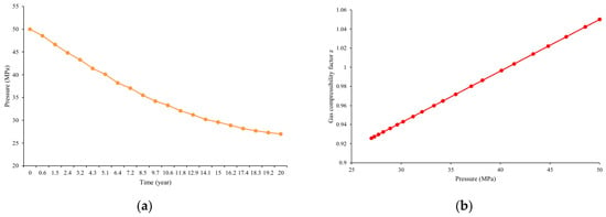
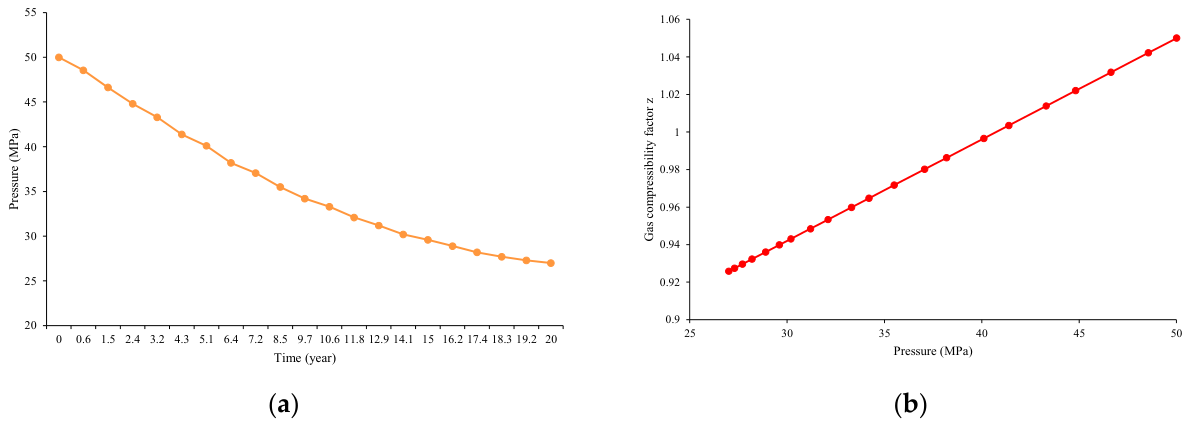
A 20-year depletion period was considered for the synthetic reservoir, during which the reservoir pressure decreased from 50 to 27 MPa. Pressure observations were distributed at irregular time intervals throughout the depletion period to represent a practical pressure-monitoring schedule. Piecewise linear interpolation was applied between adjacent measurements to construct the continuous pressure history used in the forward simulation. The resulting pressure history is presented in Figure 1a.

Figure 1. Basic input data of the synthetic reservoir model. (a) Pressure depletion history of the synthetic reservoir. (b) Pressure-dependent gas compressibility factor used in the synthetic case.

Gas PVT behavior was specified through a controlled pressure-dependent relationship. The gas compressibility factor was defined as

$$z(p)=0.78+0.0054p,$$

(35)

where p is expressed in MPa. The corresponding gas formation volume factor was calculated according to the formulation described in Section 2.2. The prescribed pressure history and pressure-dependent gas PVT properties are presented in Figure 1. The simplified PVT description was adopted to maintain internal consistency within the synthetic model rather than to represent a specific natural gas system.

3.2. Synthetic Observation Generation and Inversion Procedure

The synthetic observations were generated using the forward material balance model developed in Section 2. The reference parameters listed in Table 1 were assigned to the synthetic reservoir model, and the forward simulation was performed under the prescribed pressure history. During the simulation, the finite-aquifer response was calculated using the discrete aquifer model, and the material balance equation was subsequently solved to obtain the cumulative gas production history. The generated pressure production responses were used as synthetic observations for the subsequent inversion analysis.

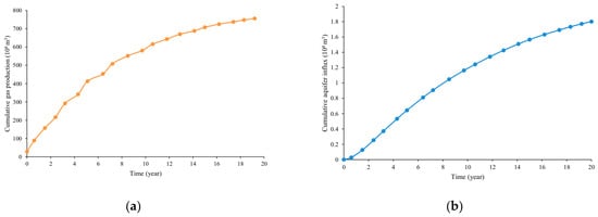
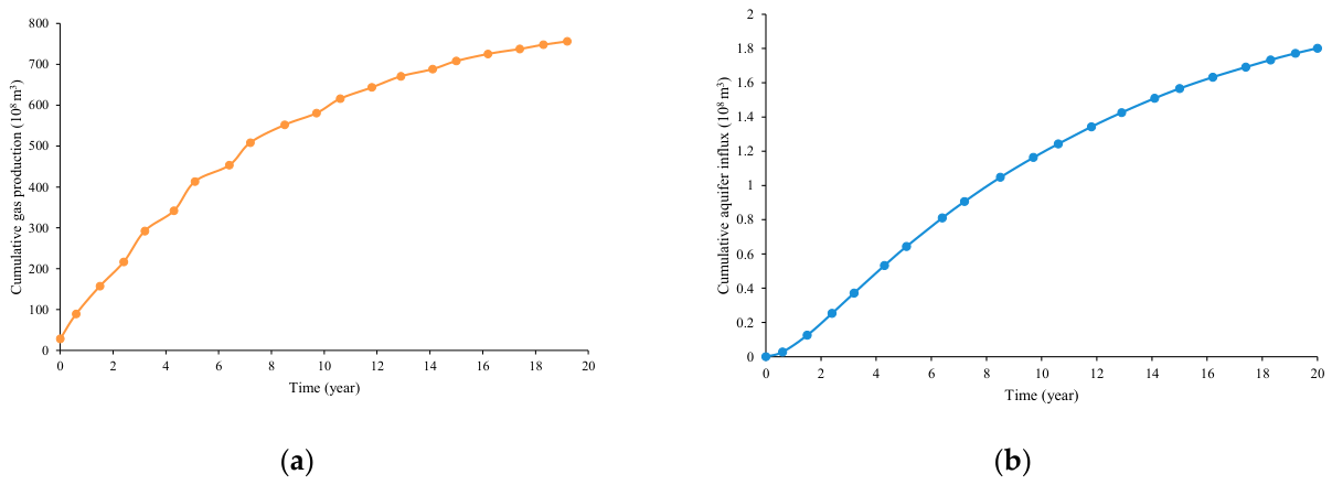
The forward-generated responses are presented in Figure 2. The cumulative gas production history shown in Figure 2a represents the production response available for inversion, whereas the cumulative aquifer influx shown in Figure 2b reflects the internal water support response calculated using the finite aquifer model. Although the cumulative aquifer influx was not directly used as an observation during inversion, its evolution provides insight into the contribution of aquifer support to the material balance response.

Figure 2. Forward-generated synthetic responses of the synthetic gas reservoir model. (a) Cumulative gas production history. (b) Cumulative aquifer influx history.

The prescribed values of the OGIP, aquifer capacitance, and response time were used for forward generation and subsequent comparison with the recovered estimates but were not supplied to the inversion. The inversion used the pressure history, cumulative gas-production observations, and the specified PVT and reservoir property inputs. At each trial τ, G and C_a were estimated using conditional linear least squares, and τ was determined from the resulting objective function profile.

3.3. Numerical Verification and Parameter Recovery

Table 2 compares the recovered parameters with the prescribed values for the noise-free synthetic case. The parameter estimates agree with the prescribed values to numerical precision, with an NRMSE on the order of 10⁻¹⁶, confirming numerical consistency between the forward and inverse implementations.

Table 2. Recovery of the prescribed synthetic parameters.

Method	G (1010 m3)	Ca (106 m3/MPa)	τ (d)	NRMSE
Reference parameters	8.5000	8.0000	400	/
Profiled inversion	8.5000	8.0000	400	3.90 × 10−16

NRMSE = normalized root mean square error.

3.4. Sensitivity Analysis Under Observation Uncertainties

The following analyses examine the parameter sensitivity to systematic production scaling, pressure measurement errors, and pressure sampling density. Conditional parameter uncertainty is further evaluated using profile likelihood confidence intervals under a specified synthetic observation error model.

3.4.1. Sensitivity to Uniform Production Scaling

Uniform multiplicative perturbations were applied to the synthetic cumulative gas production history:

$$G_p^{\ast }(t)=G_p(t)\left(1+{\epsilon }_G\right)$$

(36)

where $G_p^{*}\left(t\right)$ represents the perturbed cumulative gas production history and ε_G denotes a constant relative production-scaling perturbation applied at all observation times.

The results in Table 3 reflect the scaling structure of the material balance model. With zero water production and an unchanged pressure history, uniform scaling of cumulative gas production scales the withdrawal vector by the same factor without changing the design matrix. Consequently, the conditional estimates of G and C_a scale proportionally, while the residual sum of squares scales by the square of this factor and the location of the profile minimum remains unchanged. This explains the unchanged response time of 400 d under the prescribed production perturbations. The same scaling property holds for the constrained formulation when the production-based lower bound on G is scaled consistently. These results characterize sensitivity to systematic production scaling rather than robustness to random observation noise.

Table 3. Sensitivity to uniform production scaling and systematic pressure bias.

Case	Perturbation	G (1010 m3)	Ca (106 m3/MPa)	τ (d)
Reference	—	8.5000	8.0000	400
Production uncertainty	+5%	8.9250	8.4000	400
Production uncertainty	+10%	9.3500	8.8000	400
Production uncertainty	−5%	8.0750	7.6000	400
Production uncertainty	−10%	7.6500	7.2000	400
Pressure uncertainty	+0.2 MPa	8.7881	7.8478	340.75
Pressure uncertainty	−0.2 MPa	8.1729	8.1868	459.35
Pressure uncertainty	+0.5 MPa	9.1511	7.6792	252.31
Pressure uncertainty	−0.5 MPa	7.6221	8.5247	547.83

3.4.2. Influence of Pressure Uncertainty

The influence of systematic pressure bias was investigated by applying a constant offset to the pressure observations after the initial reference time. The perturbed pressure data are defined as

$$p^{\ast }(t)=p(t)+\Delta p$$

(37)

where p*(t) is the perturbed pressure history and Δp is the constant pressure bias. The initial reference pressure and the pressure observation at the initial time were both retained at 50 MPa. The gas compressibility and gas formation volume factors were recalculated at the perturbed pressures, while the initial gas formation volume factor remained fixed. The aquifer state was recomputed from the perturbed pressure history with zero initial aquifer depletion. The cumulative gas production remained unchanged.

The parameter estimates under different pressure biases are presented in Table 3. A positive pressure bias of 0.5 MPa decreased the estimated response time from 400 d to 252.31 d, whereas a negative bias of the same magnitude increased it to 547.83 d. G and C_a also changed, indicating that systematic pressure bias affects the inferred reservoir and aquifer parameters in the present synthetic case.

3.4.3. Effects of Random Measurement Perturbations

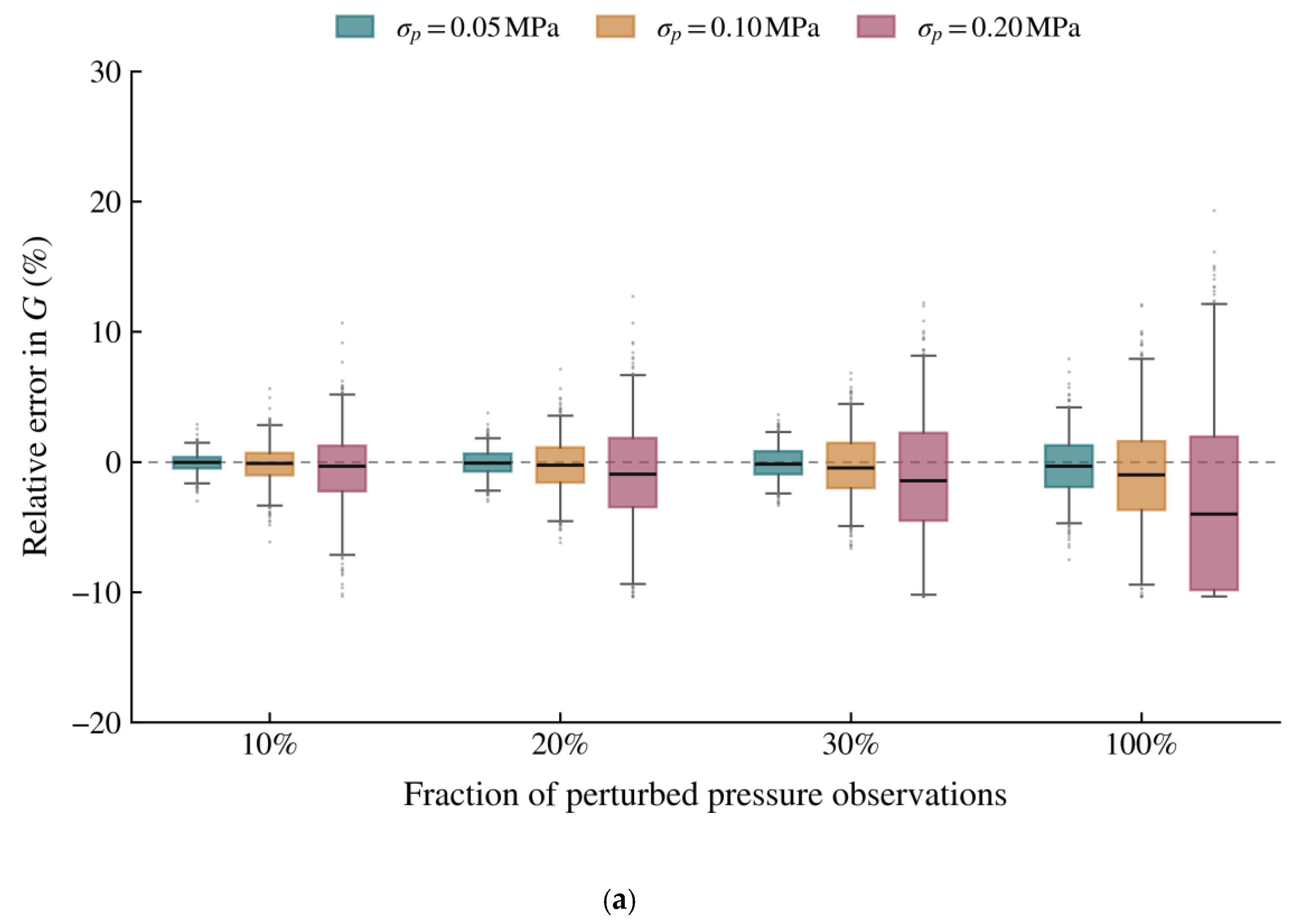
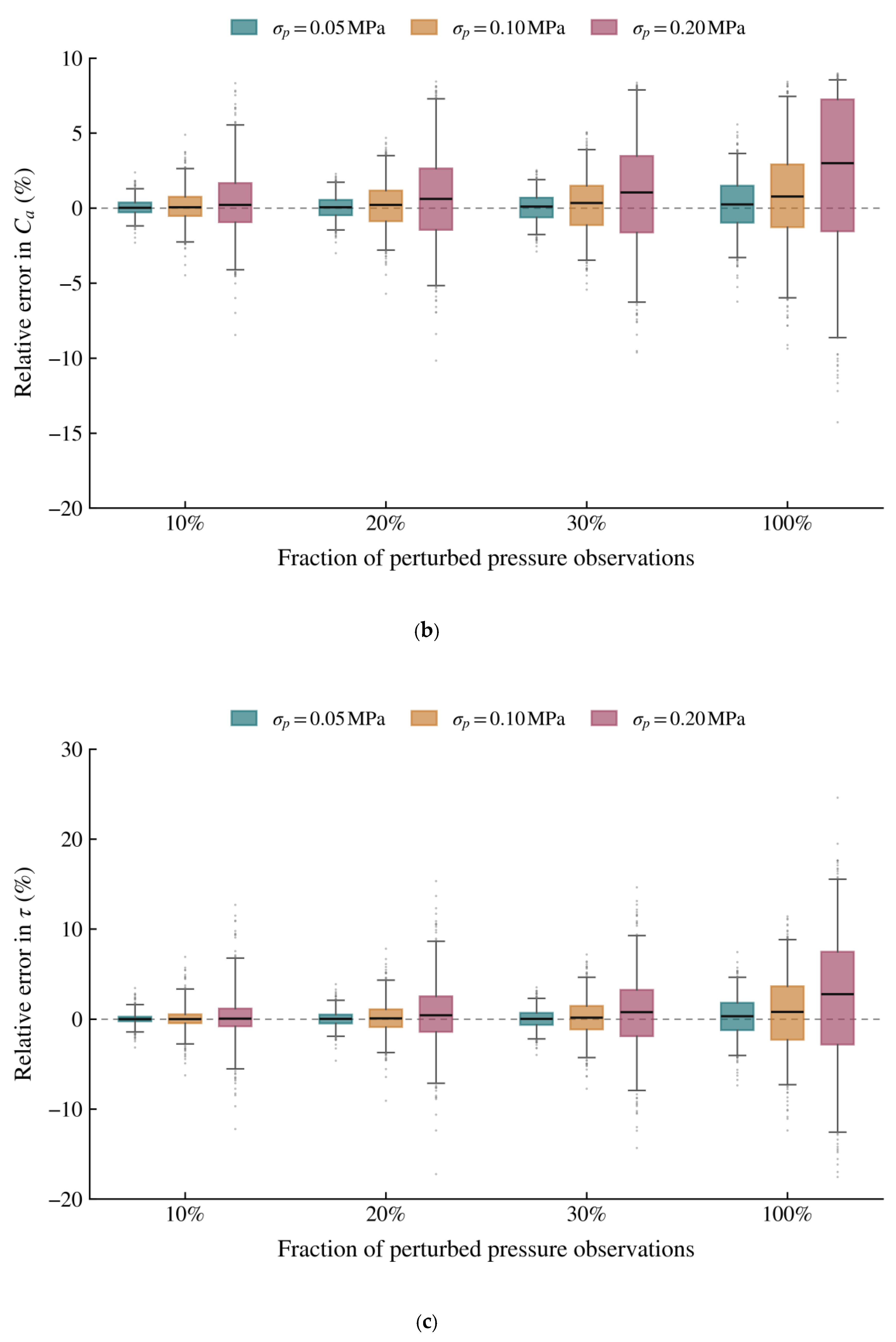
Random perturbations were introduced into selected pressure observations, while cumulative gas production and the initial pressure remained unchanged. Of the 20 noninitial pressure observations, 2, 4, or 6 was randomly selected without replacement, corresponding to a perturbation fraction of 10%, 20%, or 30%, respectively. Perturbation of all 20 observations was also considered. The perturbed pressure observations were defined as

$$\begin{array}{c}{p}_k^{\ast }=\left\{\begin{array}{cc}{p}_k+{\epsilon }_{p,k},& k\in \gamma ,\\ p_k,& k\notin \gamma ,\end{array} p_0^{\ast }=p_0\right.\\ {\epsilon }_{p,k}\stackrel{\mathrm{ind}}{\sim }N\left(0,{\sigma }_p^2\right),\hspace{1em}{\sigma }_p\in \{0.05,0.10,0.20\}\mathit{MPa}\end{array}$$

(38)

where p_k and $p_k^{*}$ are the original and perturbed pressure observations at time t_k, respectively; γ is the randomly selected set of observation indices; ε_p,k is the pressure error; and σ_p is its standard deviation.

For each perturbation fraction and error level, 500 realizations were generated. Pressure-dependent properties and the aquifer response were recalculated for each realization, and all three parameters were re-estimated using the constrained inversion. Parameter recovery was evaluated using the relative root mean square estimation error:

$$\mathit{RRMS}{E}_{\theta }=100\%\sqrt{{\displaystyle \frac{1}{M}}{\displaystyle \sum _{j=1}^M}{\left({\displaystyle \frac{\widehat{\theta }(j)-{\theta }_0}{{\theta }_0}}\right)}^2},\hspace{1em}\theta \in \left\{G,C_a,\tau \right\}$$

(39)

where M = 500 is the number of realizations, θ₀ is the prescribed parameter value, and $\widehat{\theta }(j)$ is its estimate in realization j.

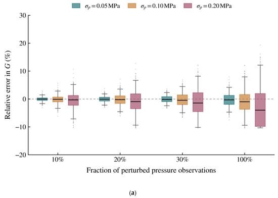
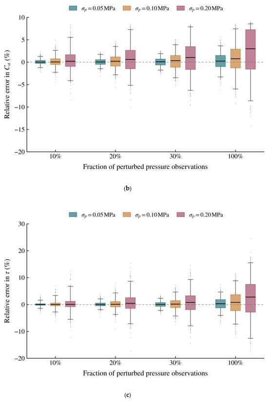
Figure 3 presents the parameter error distributions, and Table 4 summarizes the corresponding RRMSE values. Increasing the pressure error magnitude and the fraction of perturbed observations broadened the parameter distributions in the tested scenarios. At a pressure error standard deviation of 0.20 MPa, increasing the perturbation fraction from 10% to 30% increased the RRMSE from 3.10% to 4.94% for the OGIP, from 2.41% to 3.82% for the aquifer capacitance, and from 2.81% to 4.44% for the response time. When all pressure observations were perturbed at this error level, the corresponding values reached 7.36%, 5.68%, and 7.59%. These results quantify the sensitivity of parameter recovery to the magnitude and extent of random pressure errors.

Figure 3. Relative parameter-estimation errors under random pressure perturbations: (a) OGIP; (b) aquifer capacitance; (c) aquifer response time. (a) Relative error in the estimated original gas in place. (b) Relative error in the estimated aquifer capacitance. (c) Relative error in the estimated aquifer response time.

Table 4. Relative root mean square parameter-estimation errors under random pressure perturbations.

Perturbed Observations (%)	Pressure Error, σP (MPa)	RRMSE of G (%)	RRMSE of Ca (%)	RRMSE of τ (%)
10	0.05	0.77	0.60	0.71
10	0.10	1.55	1.20	1.42
10	0.20	3.10	2.41	2.81
20	0.05	1.05	0.81	0.97
20	0.10	2.11	1.63	1.95
20	0.20	4.22	3.27	3.87
30	0.05	1.25	0.97	1.12
30	0.10	2.50	1.93	2.24
30	0.20	4.94	3.82	4.44
100	0.05	2.37	1.84	2.25
100	0.10	4.49	3.48	4.32
100	0.20	7.36	5.68	7.59

3.4.4. Effect of Pressure Sampling Density

Pressure observations were progressively thinned over the same 20-year production history to examine the influence of sampling density. Nested subsets retained 100%, 90%, 80%, 70%, and 60% of the 20 noninitial observations, with the initial and final pressure points retained throughout. Pressure histories were reconstructed using piecewise linear interpolation. The OGIP and aquifer capacitance were fixed at 8.5 × 10¹⁰ m³ and 8.0 × 10⁶ m³/MPa, respectively, and only the aquifer response time was re-estimated. All cases used the same cumulative production records and residual evaluation times, with the pressure-dependent properties and aquifer response recalculated for each subset.

Table 5 summarizes the results. Reducing the retained fraction from 100% to 60% increased the mean sampling interval from 365.00 to 608.33 d and decreased the estimated response time from 400.00 to 391.75 d, corresponding to a relative error of −2.06%. For this synthetic history, pressure thinning produced a modest downward shift in the response time estimate, with absolute relative errors remaining within 2.06% under the prescribed fixed-parameter conditions.

Table 5. Effects of pressure sampling density on the estimated aquifer response time.

Retained (%)	Pressure Points	Mean Interval (d)	Max. Interval (d)	Estimated τ (d)	Error (%)
100	21	365.00	474.50	400.00	0.00
90	19	405.56	620.50	397.22	−0.70
80	17	456.25	693.50	394.87	−1.28
70	15	521.43	766.50	393.12	−1.72
60	13	608.33	766.50	391.75	−2.06

3.4.5. Profile-Likelihood Confidence Intervals

Parameter uncertainty was evaluated using a synthetic example with an exact pressure history and independent, zero-mean Gaussian errors added to the material balance withdrawal observations. The known error standard deviation was set to 1% of the mean noise-free withdrawal over the 20 noninitial observations. Each parameter was fixed in turn while the other two were re-optimized within the adopted physical bounds. Approximate 95% confidence intervals were determined using a profile likelihood-ratio threshold of 3.841, corresponding to one degree of freedom [26].

Table 6 summarizes the parameter estimates and intervals. The prescribed values fall within their respective intervals for this realization. The lower endpoint of the OGIP interval coincides with the production-based physical bound and is therefore constraint-determined. These intervals quantify parameter uncertainty under the specified synthetic error model, complementing the preceding input-sensitivity analyses and the parameter trade-off analysis in Section 3.5.

Table 6. Parameter estimates and approximate 95% confidence intervals for the synthetic example.

Parameter	Unit	Prescribed Value	Estimate	95% Interval
G	1010 m3	8.5000	8.0301	[7.6245,9.5736]
Ca	106 m3/MPa	8.0000	8.3508	[7.2428,8.7202]
τ	d	400.00	394.20	[331.86,447.39]

3.5. Parameter Profiles and Trade-Off Analysis

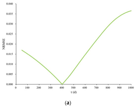
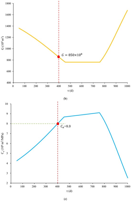
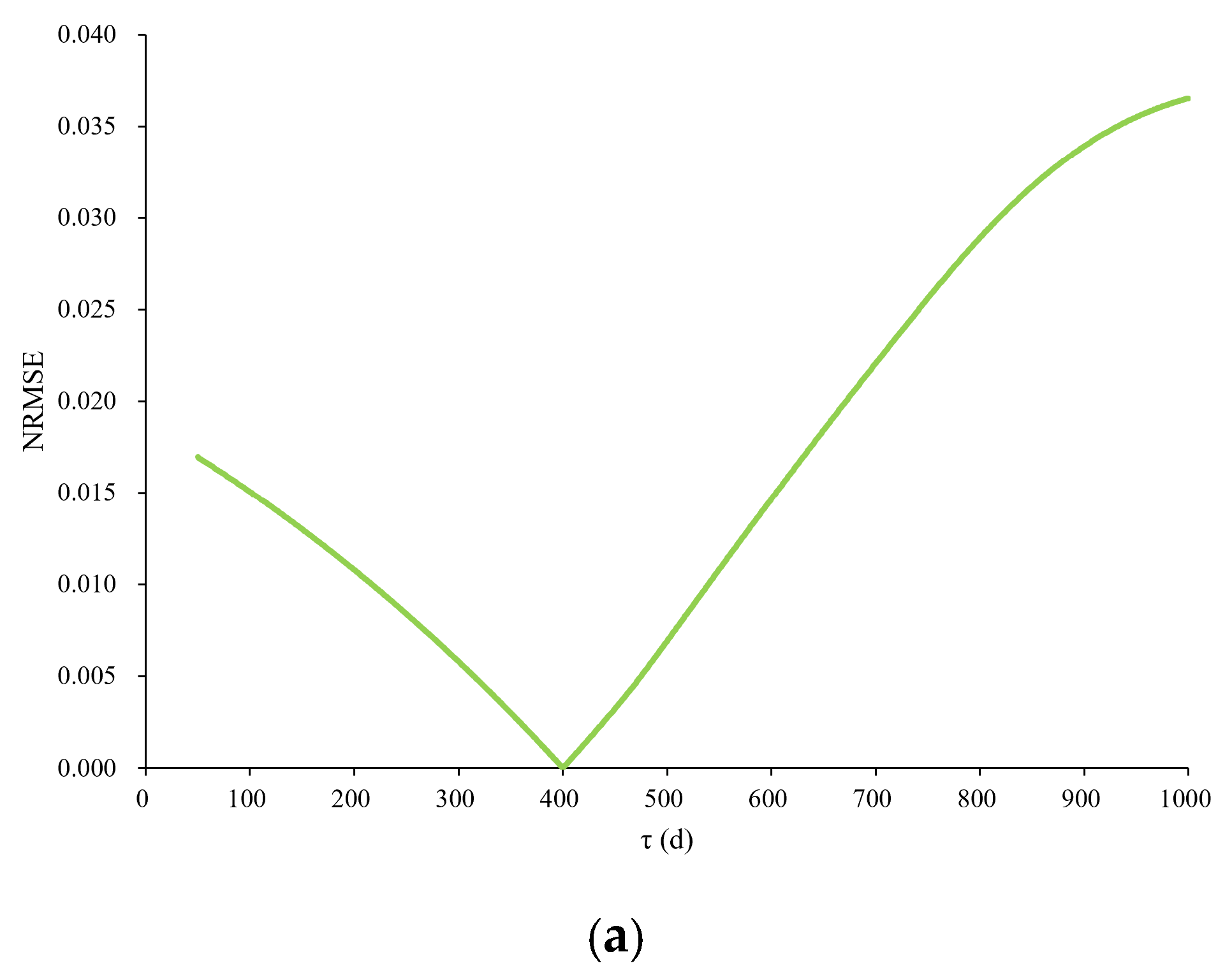
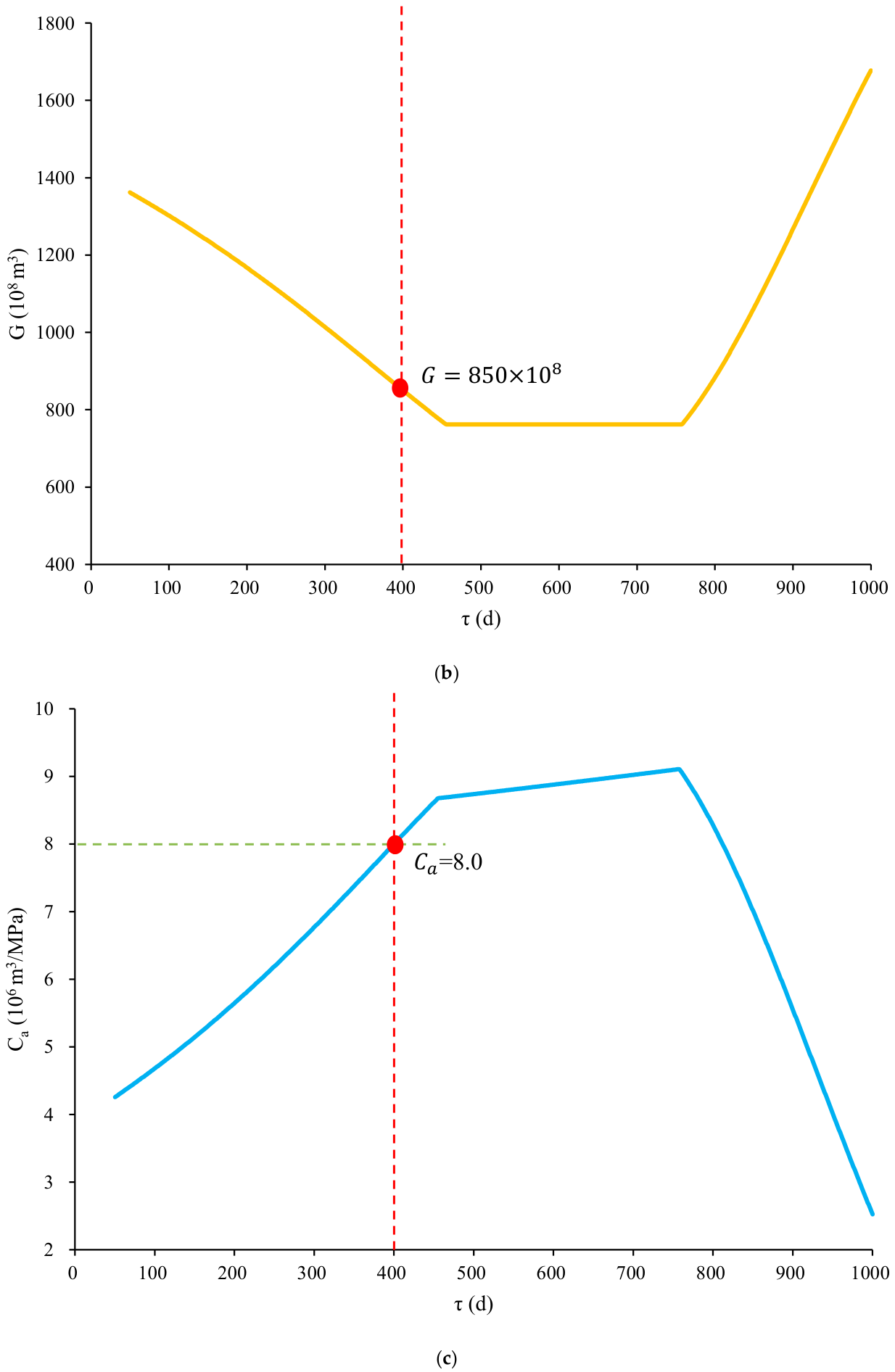
Figure 4 presents the residual and conditional parameter profiles of the noise-free synthetic case under the adopted physical constraints. The residual profile shown in Figure 4a reached its minimum at a response time of 400 d.

Figure 4. Parameter profile characteristics of the aquifer response time. (a) Objective function profile with respect to τ. (b) Variation in optimized G along the parameter profile. (c) Variation in optimized C_a along the parameter profile.

Figure 4b,c show the corresponding parameter adjustments. As the trial response time increased, the conditional OGIP estimate decreased and reached the production-based lower bound at approximately 455.18 d. It remained at this bound until approximately 755.89 d, forming a plateau, while the aquifer capacitance continued to increase. Beyond this interval, the OGIP estimate rose above the bound and the capacitance decreased. These profiles illustrate how the physical constraint modifies the compensating relationship between the OGIP and aquifer capacitance as the assumed response time changes.

4. Field Application and Parameter Constraint Analysis

The proposed inversion framework was applied to a water-drive gas reservoir to estimate the OGIP and effective aquifer parameters. The results were assessed through historical production reconstruction, residual evaluation, parameter profile analysis, and checks of the reconstructed histories against the physical admissibility criteria in Section 2.7. The effect of incorporating the reference OGIP is examined separately in Section 4.2.

4.1. Reservoir Data and Data Processing

The field case was a water-drive porous gas reservoir. The reservoir identity and absolute OGIP are withheld for confidentiality. The analysis used reservoir-scale pressure and production records, together with the available fluid property data.

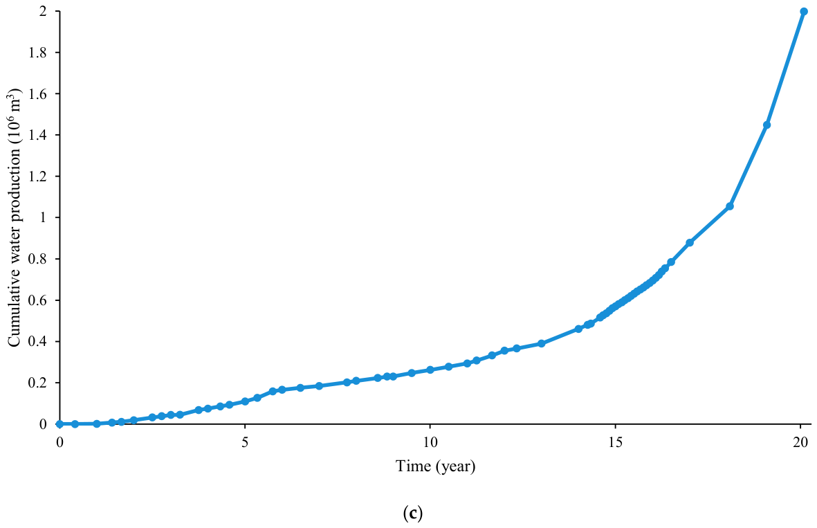
The dataset comprised one initial reference point and 63 subsequent observation points over approximately 20 years. The available inputs included the average reservoir pressure, cumulative gas production, cumulative water production, and gas formation volume factors corresponding to the observed pressures. The pressure and production data were obtained from field records.

The reference OGIP, G_ref, was provided by the field operator as the mean of the gas-in-place estimates obtained using a binomial material balance analysis, the apparent-gas-in-place method, and estimation based on gas production per unit pressure decline. Relative to this mean, the minimum and maximum estimates are approximately 2.89% lower and 1.97% higher, respectively.

For graphical comparison, the following variables were normalized using their initial or reference values. The dimensionless pressure, cumulative gas production, and gas formation volume factor are defined as

$$p^{\ast }={\displaystyle \frac{p}{p_i}}, G_p^{\ast }={\displaystyle \frac{G_p}{G_{\mathit{ref}}}}, B_g^{\ast }={\displaystyle \frac{B_g}{B_{\mathit{gi}}}}$$

(40)

where G_ref represents the reference gas-in-place value used for normalization, and B_gi denotes the initial gas formation volume factor.

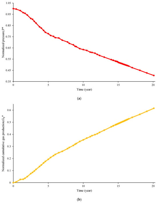
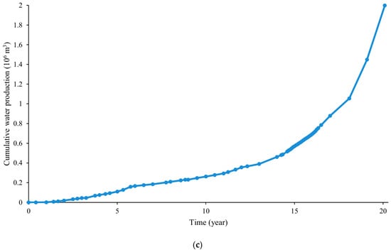
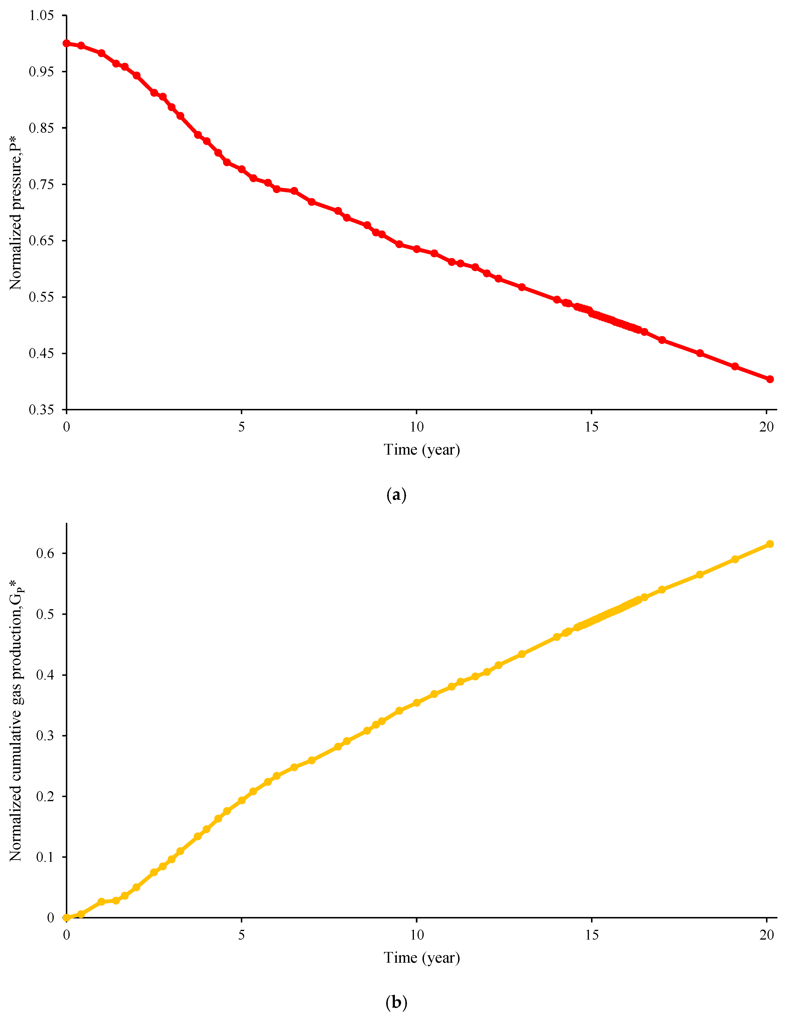
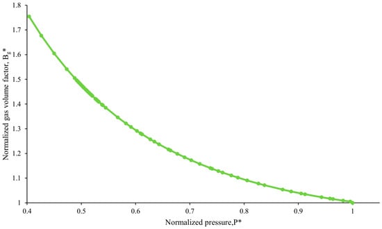
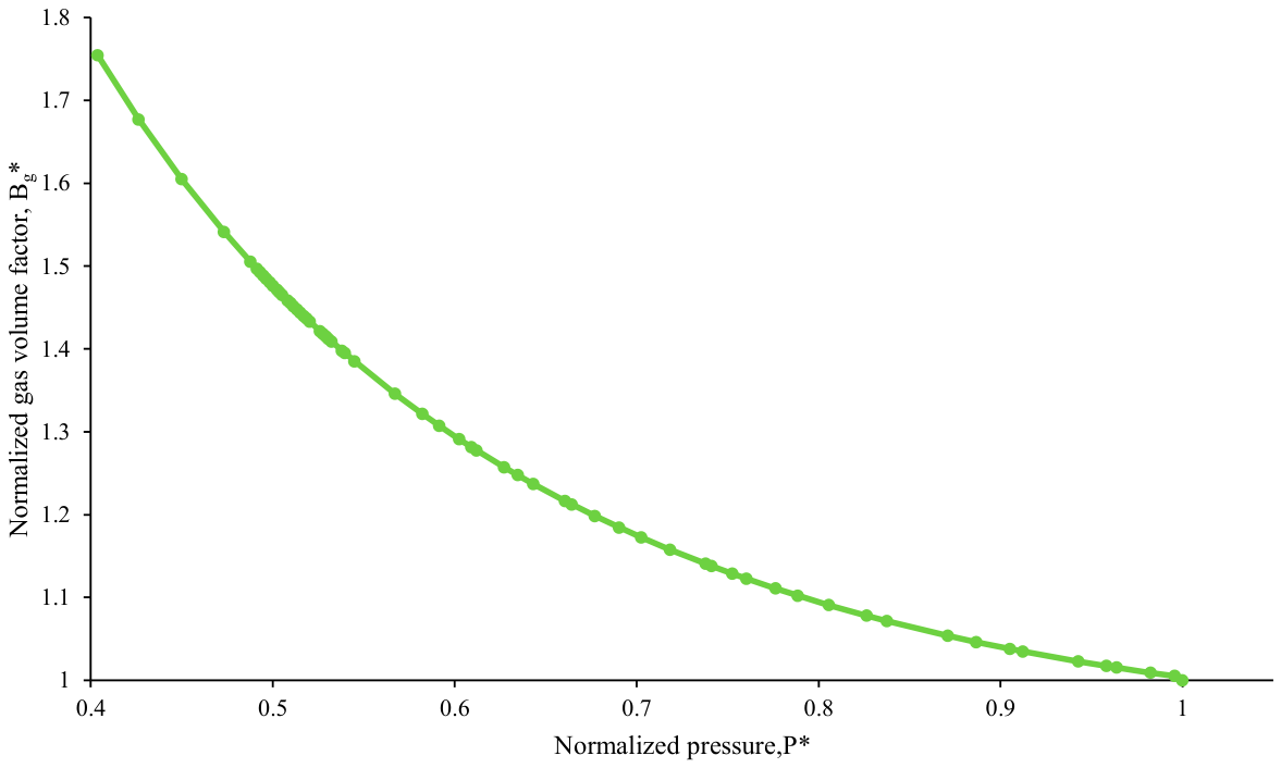
All inversion calculations used the original field data. Figure 5a–c present the normalized pressure and cumulative gas production histories, together with cumulative water production. Figure 6 shows the relationship between the normalized gas formation volume factor and normalized pressure. The basic parameters used in the field calculation are summarized in Table 7.

Figure 5. (a) Normalized reservoir pressure history. (b) Normalized cumulative gas production history. (c) Cumulativewater production history.

Figure 6. Relationship between normalized gas formation volume factor and normalized pressure.

Table 7. Basic parameters used in the field calculation.

Parameter	Symbol	Value	Unit
Production history nodes	N	63	/
Production history duration	/	20	year
Initial water saturation	Swi	0.32	/
Rock compressibility	cf	1.423 × 10−3	MPa−1
Water compressibility	cw	4.0 × 10−4	MPa−1
Water formation volume factor	Bw	1.00358	-

4.2. Inversion Results and Historical Production Reconstruction

The field application examined parameter estimates under two OGIP scenarios and the agreement between the reconstructed and observed cumulative gas production.

4.2.1. Parameter Inversion and Physical Consistency

The field inversion results are summarized in Table 8. Two scenarios were considered: one in which the OGIP was estimated together with the aquifer parameters, and another in which the OGIP was fixed at the reference value. In the first scenario, G and C_a were estimated using bounded conditional linear least squares at each trial response time, subject to G ≥ max G_p,k and C_a ≥ 0. In the second scenario, G was fixed at G_ref, and only C_a was estimated conditionally at each trial response time, subject to C_a ≥ 0. The response time was determined separately for each scenario from its corresponding objective function profile.

Table 8. Parameter estimates for the two OGIP scenarios.

Scenario	G/Gref	Ca (m3/MPa)	τ (d)	NRMSE
OGIP estimated	1.006655	3.5912 × 106	386.94	0.009375
OGIP fixed at Gref	1.0000	3.67 × 106	402	0.009389

The estimated OGIP was approximately 0.67% higher than the field reference value, with G/G_ref = 1.006655, and lay within the field evaluation range described in Section 4.1. This agreement supports the applicability of the proposed method to OGIP evaluation in this field case. The estimated aquifer capacitance was positive in both scenarios.

4.2.2. Historical Production Reconstruction

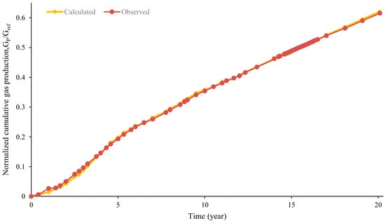
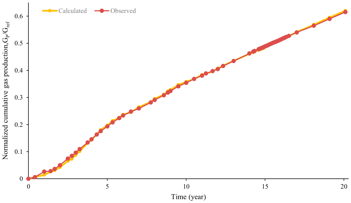
Using the parameters obtained from the field inversion, the finite-aquifer material balance model was applied to reconstruct the historical cumulative gas production. The pressure and production records used for this reconstruction were the same records used for parameter estimation. Accordingly, Figure 7 demonstrates the consistency with the historical data used for fitting and does not provide independent validation of the estimated parameters.

Figure 7. Comparison between observed and reconstructed cumulative gas production.

Figure 7 shows that the reconstructed cumulative gas production follows the observed production trend throughout the analyzed period. The material balance NRMSE values reported in Table 8 are 0.009375 and 0.009389 for the estimated-OGIP and fixed-OGIP scenarios, respectively. These close values indicate a limited change in the reported fitting error when the OGIP was fixed at the reference value in this field case.

To examine the temporal variation in the reconstruction error, the normalized residual of cumulative gas production was calculated using

$${\displaystyle \frac{\Delta G_p}{G_{\mathrm{ref}}}}={\displaystyle \frac{G_{p,\mathit{obs}}-G_{p,\mathrm{rec}}}{G_{\mathrm{ref}}}}$$

(41)

where G_p,obs and G_p,rec denote the observed and reconstructed cumulative gas production, respectively.

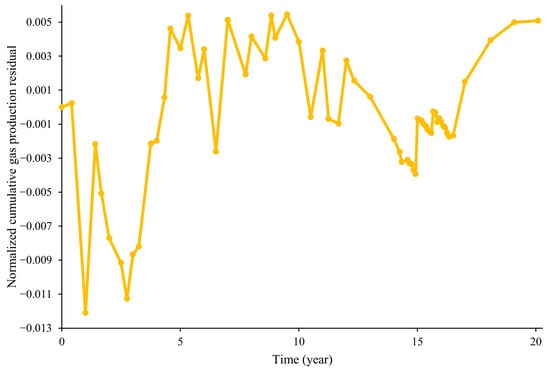
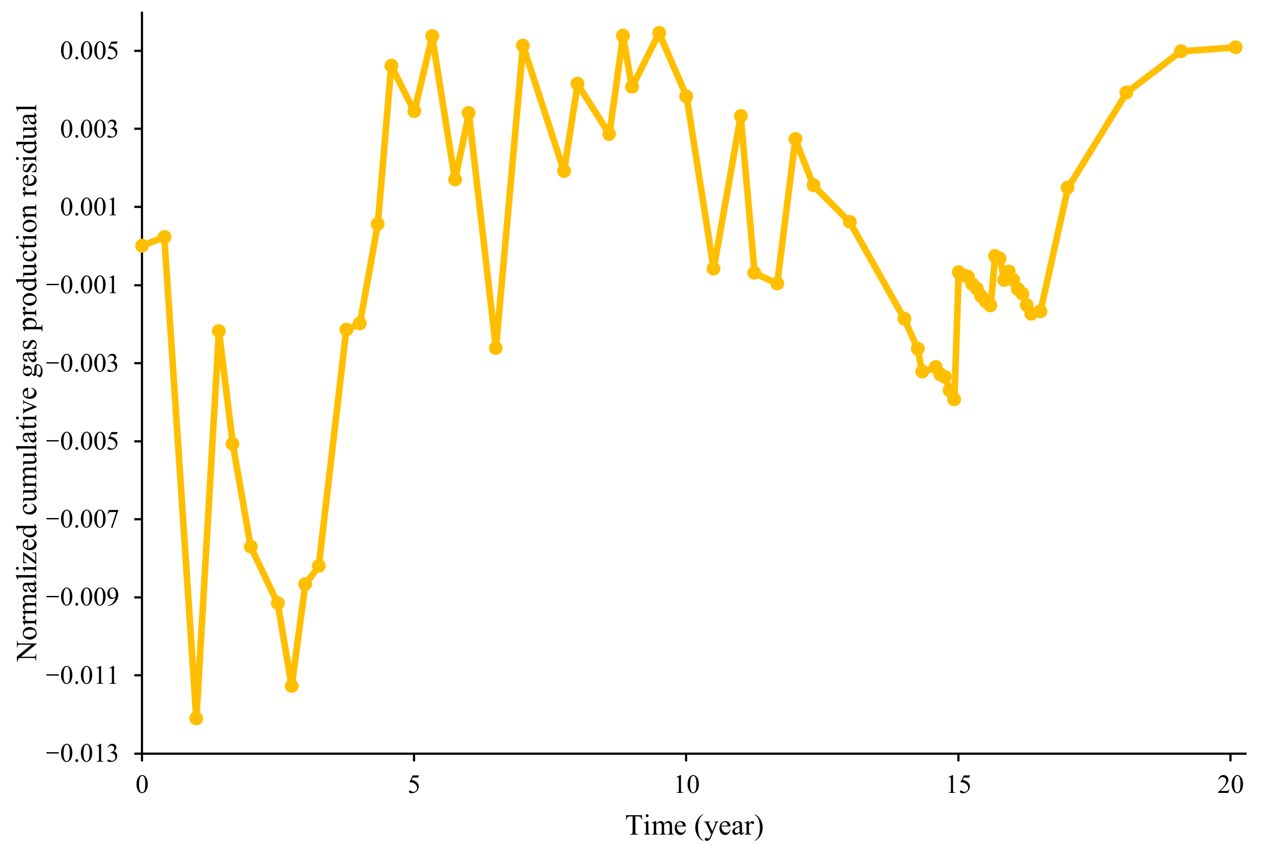
The normalized residual distribution is presented in Figure 8, with values ranging approximately from −1.2 × 10⁻² to 5.4 × 10⁻³. The residuals exhibit sustained positive or negative deviations over several intervals, indicating temporal patterns in the reconstruction error despite agreement with the overall production trend.

Figure 8. Normalized residual distribution of reconstructed cumulative gas production.

4.3. Parameter Stability and Sensitivity Analysis

Objective function and parameter profiles were examined to characterize the response time sensitivity and parameter trade-offs. The effects of water production and reservoir elastic expansion were assessed by omitting each term separately and repeating the inversion.

4.3.1. Profile Analysis of Aquifer Response Time

For the estimated-OGIP scenario, the objective function and conditional parameter profiles were constructed by varying the aquifer response time τ over the prescribed range. At each trial value, G and C_a were re-estimated using the bounded conditional linear least squares procedure described in Section 2.5.

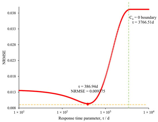
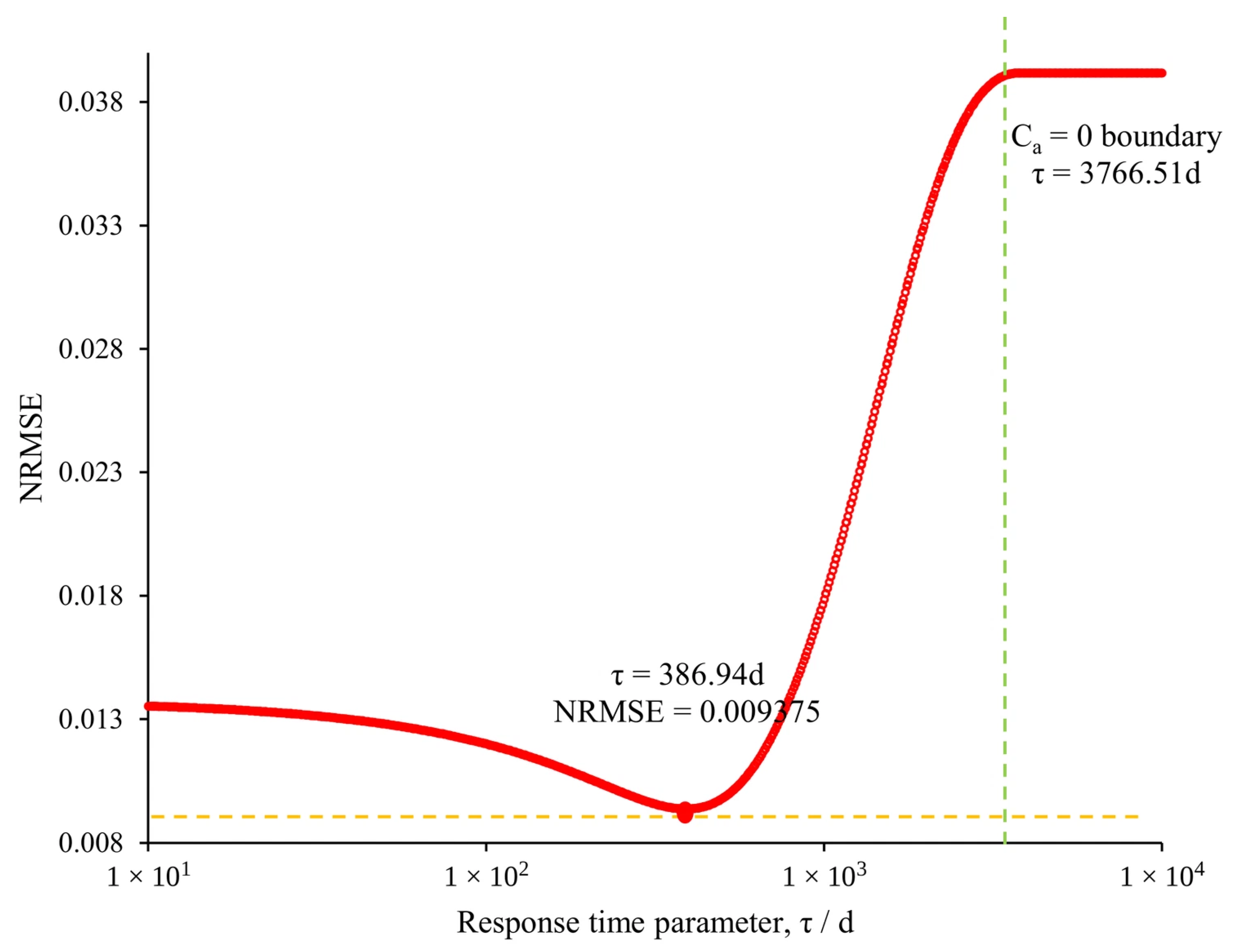
Figure 9 shows that NRMSE = 0.009375 at τ = 386.94d, consistent with the inversion results reported in Table 8. Before the capacitance bound became active, the NRMSE initially decreased and then increased with increasing τ, indicating the response time sensitivity of the objective function for the observed pressure–production history within the adopted finite aquifer model.

Figure 9. Constrained objective function profile with respect to aquifer response time.

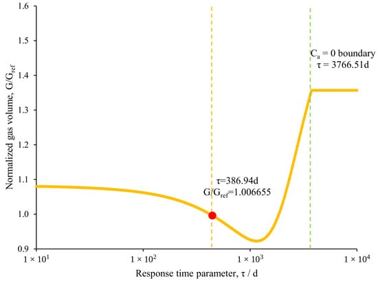
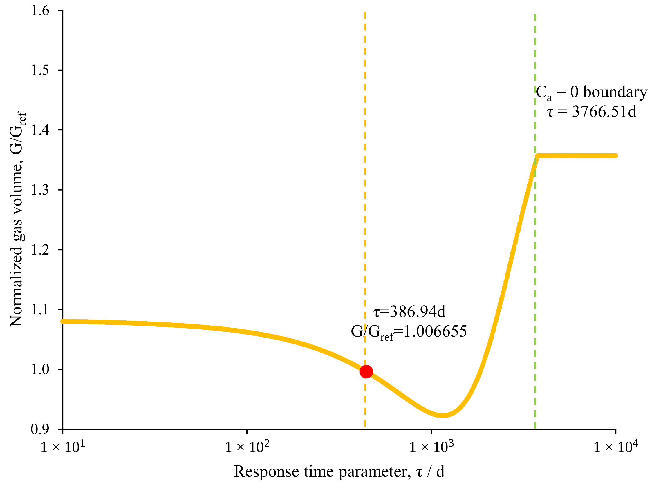
Figure 10 presents the variation in the normalized gas volume parameter G/G_ref with respect to the response time τ. The gas volume parameter exhibited a nonmonotonic dependence on τ, reflecting compensating adjustments in the conditional parameter estimates. At the response time estimate of τ = 386.94 d, the estimated gas volume was close to the reference value, with G/G_ref = 1.006655.

Figure 10. Bounded conditional profile of normalized gas volume with respect to aquifer response time.

Similar G/G_ref values may occur at different response times because the linear parameters were re-estimated for each prescribed τ. Therefore, the gas volume profile alone cannot determine the response time and should be interpreted together with the constrained objective function profile in Figure 9.

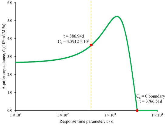
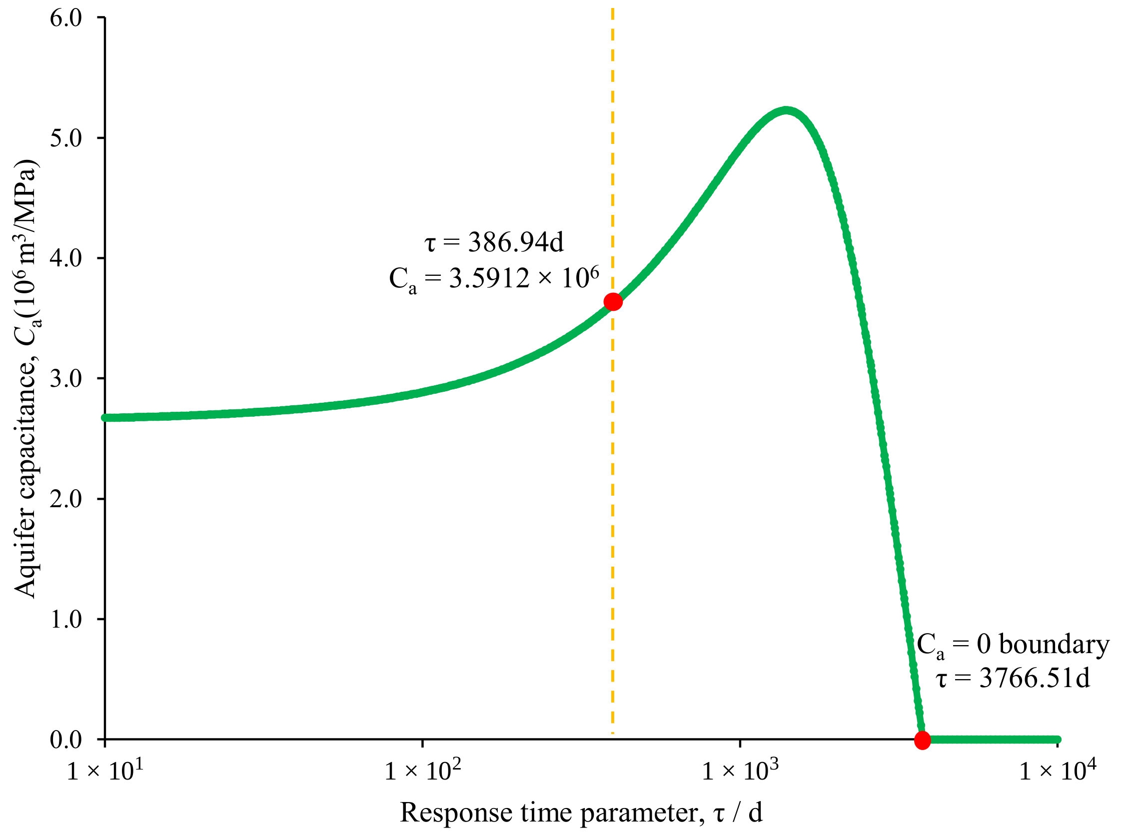
The bounded conditional profile of the aquifer capacitance C_a with respect to the response time τ is shown in Figure 11. Its variation reflects compensating adjustments in the aquifer storage capacity as the response time changed. At the response time estimate of τ = 386.94 d, C_a = 3.5912 × 10⁶ m³/MPa, where the nonnegative capacitance bound was inactive at this point.

Figure 11. Bounded conditional profile of aquifer capacitance with respect to aquifer response time.

Within the investigated range, the conditional capacitance estimate reached its lower bound, C_a = 0, at approximately τ = 3766.51 d and remained at zero for larger response times. The water influx term then vanished, making the material balance relation independent of τ. Consequently, the objective function and estimated OGIP remained constant, producing the plateaus shown in Figure 9 and Figure 10, respectively. Under this boundary condition, the aquifer response time cannot be determined from the available observations.

4.3.2. Influence of Physical Terms

The complete material balance formulation accounted for gas expansion, reservoir and connate water elastic expansion, finite aquifer influx, and produced-water withdrawal. Two simplified cases were evaluated by omitting the water production term and the elastic expansion term separately and repeating the inversion using the field dataset. The resulting parameter estimates are summarized in Table 9.

Table 9. Comparison of inversion results under different physical assumptions.

Case	G/Gref	Ca (m3/MPa)	τ (d)	NRMSE
Complete model	1.006655	3.5912 × 106	386.94	0.009375
Without water production term	0.999761	3.6468 × 106	394.45	0.009522
Without elastic expansion term	1.020563	4.9564 × 106	221.60	0.010097

Relative to the complete model, omitting the water production term decreased the estimated G by approximately 0.685%, increased C_a by 1.55%, and increased τ by 1.94%. These changes indicate a modest influence of produced-water withdrawal on the recovered parameters in the present field case.

Omitting the elastic expansion term increased the OGIP by approximately 1.38% and aquifer capacitance by 38.0%, while decreasing the response time by 42.7%. During pressure depletion, pore volume contraction and connate water expansion contributed to the withdrawal balance. In the adopted formulation, this contribution followed the pressure depletion directly, whereas the aquifer influx depended on the preceding pressure history and exhibited a response lag. When the elastic contribution was omitted, the inversion was compensated through increased gas expansion and stronger aquifer support. The higher OGIP increased the gas expansion contribution, while the larger aquifer capacitance increased the magnitude of aquifer influx. The shorter response time reduced the lag of aquifer support, which allowed the calculated influx to follow the pressure depletion more closely and partly replace the omitted elastic contribution. These coordinated adjustments explain the inferred increase in capacitance and decrease in response time in the present field case. The accompanying increase in NRMSE from 0.009375 to 0.010097 further supports retaining the elastic expansion term in this application.

The comparison shows that in this field case, omission of reservoir and connate water elastic expansion has a greater influence on the estimated aquifer parameters than omission of produced-water withdrawal.

4.4. Discussion

The comparison between the two OGIP scenarios illustrates how an existing reserve estimate can be incorporated into aquifer evaluation within the same material balance formulation. Estimating the OGIP yields a gas volume estimate close to the operator’s reference evaluation, while fixing OGIP at that reference produces little change in the fitting error. The formulation can therefore accommodate the joint estimation of reservoir and aquifer parameters and an aquifer evaluation conditioned on an existing OGIP estimate, depending on the information available for the field.

The parameter profiles and physical term comparison highlight the dependence of the inferred aquifer response on the adopted model representation. With the field observations unchanged, aquifer parameter adjustments in the term-omission cases partly compensate for changes in the retained material-balance contributions. Aquifer capacitance and response time consequently describe the effective aquifer behavior represented by the model over the observed production history. Consistent treatment of reservoir elastic contributions, water influx, and produced-water withdrawal is therefore important when interpreting and comparing these parameter estimates.

5. Conclusions

The following conclusions were drawn from this study:

(1).

Exploiting the separable parameter structure of the finite-aquifer material balance equations reduces the nonlinear inversion to a one-dimensional search over the aquifer response time, with bounded conditional linear estimation of the original gas in place (OGIP) and aquifer capacitance. The objective function and conditional parameter profiles characterize the residual sensitivity, parameter trade-offs, and influence of active physical bounds.

(2).

The noise-free synthetic case recovered the prescribed parameters to numerical precision. When random pressure errors with a standard deviation of 0.20 MPa were applied to 30% of the noninitial pressure observations, the relative root mean square estimation errors were 4.94%, 3.82%, and 4.44% for the OGIP, aquifer capacitance, and response time, respectively. The profile likelihood analysis additionally provided approximate 95% confidence intervals under the specified withdrawal error model.

(3).

With the OGIP and aquifer capacitance fixed, retaining 60% of the noninitial pressure observations shifted the estimated response time from 400.00 to 391.75 d, corresponding to a relative error of −2.06%. This result characterizes the effect of pressure thinning under the prescribed synthetic conditions.

(4).

The field application yielded an aquifer response time of 386.94 d, aquifer capacitance of 3.5912 × 10⁶ m³/MPa, and NRMSE of 0.009375. The estimated OGIP was approximately 0.67% above the operator-provided reference value and within the range of the existing field evaluations, supporting the formulation’s applicability to OGIP evaluation in this field case.

References

- Havlena, D.; Odeh, A.S. The material balance as an equation of a straight line. J. Pet. Technol. 1963, 15, 896–900. [Google Scholar] [CrossRef] [Scilit]
- Agarwal, R.G.; Al-Hussainy, R.; Ramey, H.J., Jr. The importance of water influx in gas reservoirs. J. Pet. Technol. 1965, 17, 1336–1342. [Google Scholar] [CrossRef] [Scilit]
- Bruns, J.R.; Fetkovich, M.J.; Meitzen, V.C. The effect of water influx on p/z–cumulative gas production curves. J. Pet. Technol. 1965, 17, 287–291. [Google Scholar] [CrossRef] [Scilit]
- Pletcher, J.L. Improvements to reservoir material-balance methods. SPE Reserv. Eval. Eng. 2002, 5, 49–59. [Google Scholar] [CrossRef] [Scilit]
- Elahmady, M.; Wattenbarger, R.A. A straight-line p/z plot is possible in waterdrive gas reservoirs. In Proceedings of the SPE Rocky Mountain Oil & Gas Technology Symposium, Denver, CO, USA, 16–18 April 2007. [Google Scholar] [CrossRef]
- van Everdingen, A.F.; Hurst, W. The application of the Laplace transformation to flow problems in reservoirs. J. Pet. Technol. 1949, 1, 305–324. [Google Scholar] [CrossRef] [Scilit]
- Carter, R.D.; Tracy, G.W. An improved method for calculating water influx. Trans. AIME 1960, 219, 415–417. [Google Scholar] [CrossRef] [Scilit]
- Fetkovich, M.J. A simplified approach to water influx calculations—Finite aquifer systems. J. Pet. Technol. 1971, 23, 814–828. [Google Scholar] [CrossRef] [Scilit]
- Yildiz, T.; Khosravi, A. An analytical bottomwaterdrive aquifer model for material-balance analysis. SPE Res. Eval. Eng. 2007, 10, 618–628. [Google Scholar] [CrossRef] [Scilit]
- McEwen, C.R. Material balance calculations with water influx in the presence of uncertainty in pressures. Soc. Pet. Eng. J. 1962, 2, 120–128. [Google Scholar] [CrossRef] [Scilit]
- Chierici, G.L.; Pizzi, G.; Ciucci, G.M. Water drive gas reservoirs: Uncertainty in reserves evaluation from past history. J. Pet. Technol. 1967, 19, 237–244. [Google Scholar] [CrossRef] [Scilit]
- Sills, S.R. Improved material-balance regression analysis for waterdrive oil and gas reservoirs. SPE Res. Eng. 1996, 11, 127–134. [Google Scholar] [CrossRef] [Scilit]
- Vega, L.; Wattenbarger, R.A. New approach for simultaneous determination of the OGIP and aquifer performance with no prior knowledge of aquifer properties and geometry. In Proceedings of the SPE/CERI Gas Technology Symposium, Calgary, AB, Canada, 3–5 April 2000. [Google Scholar] [CrossRef]
- Yildiz, T. A hybrid approach to improve reserves estimates in waterdrive gas reservoirs. SPE Res. Eval. Eng. 2008, 11, 696–706. [Google Scholar] [CrossRef] [Scilit]
- Garcia, C.A.; Villa, J.R. Pressure and PVT uncertainty in material-balance calculations. In Proceedings of the SPE Latin American & Caribbean Petroleum Engineering Conference, Buenos Aires, Argentina, 15–18 April 2007. [Google Scholar] [CrossRef]
- Kabir, C.S.; Parekh, B.; Mustafa, M.A. Material-balance analysis of gas and gas-condensate reservoirs with diverse drive mechanisms. J. Nat. Gas Sci. Eng. 2016, 32, 158–173. [Google Scholar] [CrossRef] [Scilit]
- Zavaleta, S.; Adrian, P.M.; Michel, M. Estimation of OGIP in a water-drive gas reservoir coupling dynamic material balance and Fetkovich aquifer model. In Proceedings of the SPE Trinidad and Tobago Section Energy Resources Conference, Port of Spain, Trinidad and Tobago, 25–26 June 2018. [Google Scholar] [CrossRef] [Scilit]
- Yu, Q.; Hu, X.; Liu, P.; Jia, Y.; Li, Y. Researches on calculation methods of aquifer influx for gas reservoirs with aquifer support. J. Pet. Sci. Eng. 2019, 177, 889–898. [Google Scholar] [CrossRef] [Scilit]
- Jongkittinarukorn, K.; Kabir, C.S. A novel material-balance approach for estimating in-place volumes of gas and water in gas reservoirs with aquifer support. J. Pet. Explor. Prod. Technol. 2023, 13, 1627–1640. [Google Scholar] [CrossRef] [Scilit]
- Yuan, H.; Wang, J. Universal material balance equation for the analysis of condensate gas reservoirs with edgewater and bottomwater drive aquifer. AIP Adv. 2025, 15, 115019. [Google Scholar] [CrossRef] [Scilit]
- Li, H.; Zhu, S.; Peng, X.; Wang, P.; Xing, C.; Yan, C.; Wang, K. A water influx calculation model incorporating dissolved gas evolution and residual gas expansion and its application to the W gas field. Processes 2026, 14, 2296. [Google Scholar] [CrossRef] [Scilit]
- Meng, F.; Liu, Y.; Liu, X.; Duan, C.; Zhou, Y. A multi-block material balance framework for connectivity evaluation and optimization of water-drive gas reservoirs. Fluid Dyn. Mater. Process. 2026, 22, 3. [Google Scholar] [CrossRef] [Scilit]
- Golub, G.H.; Pereyra, V. The differentiation of pseudo-inverses and nonlinear least squares problems whose variables separate. SIAM J. Numer. Anal. 1973, 10, 413–432. [Google Scholar] [CrossRef] [Scilit]
- O’Leary, D.P.; Rust, B.W. Variable projection for nonlinear least squares problems. Comput. Optim. Appl. 2013, 54, 579–593. [Google Scholar] [CrossRef] [Scilit]
- von Schroeter, T.; Hollaender, F.; Gringarten, A.C. Deconvolution of well-test data as a nonlinear total least-squares problem. SPE J. 2004, 9, 375–390. [Google Scholar] [CrossRef] [Scilit]
- Raue, A.; Kreutz, C.; Maiwald, T.; Bachmann, J.; Schilling, M.; Klingmüller, U.; Timmer, J. Structural and practical identifiability analysis of partially observed dynamical models by exploiting the profile likelihood. Bioinformatics 2009, 25, 1923–1929. [Google Scholar] [CrossRef] [Scilit] [PubMed]
Disclaimer/Publisher’s Note: The statements, opinions and data contained in all publications are solely those of the individual author(s) and contributor(s) and not of MDPI and/or the editor(s). MDPI and/or the editor(s) disclaim responsibility for any injury to people or property resulting from any ideas, methods, instructions or products referred to in the content. |
© 2026 by the authors. Licensee MDPI, Basel, Switzerland. This article is an open access article distributed under the terms and conditions of the Creative Commons Attribution (CC BY) license.